Contractions of Quantum Superintegrable Systems and the Askey Scheme

Contractions of 2D 2nd Order Quantum
Superintegrable Systems and the Askey Scheme
for Hypergeometric Orthogonal Polynomials

Ernest G. KALNINS ^†, Willard MILLER Jr. ^‡ and Sarah POST ^§

E.G. Kalnins, W. Miller Jr. and S. Post

^† Department of Mathematics, University of Waikato, Hamilton, New Zealand math0236@waikato.ac.nz

^‡ School of Mathematics, University of Minnesota, Minneapolis, MN, 55455, USA miller@ima.umn.edu

^§ Department of Mathematics, U. Hawai‘i at Manoa, Honolulu, HI, 96822, USA spost@hawaii.edu

Received May 29, 2013, in final form September 26, 2013; Published online October 02, 2013

We show explicitly that all 2nd order superintegrable systems in 2 dimensions are limiting cases of a single system: the generic 3-parameter potential on the 2-sphere, ${\rm S}9$ in our listing. We extend the Wigner–Inönü method of Lie algebra contractions to contractions of quadratic algebras and show that all of the quadratic symmetry algebras of these systems are contractions of that of ${\rm S}9$. Amazingly, all of the relevant contractions of these superintegrable systems on flat space and the sphere are uniquely induced by the well known Lie algebra contractions of e(2) and so(3). By contracting function space realizations of irreducible representations of the ${\rm S}9$ algebra (which give the structure equations for Racah/Wilson polynomials) to the other superintegrable systems, and using Wigner’s idea of “saving” a representation, we obtain the full Askey scheme of hypergeometric orthogonal polynomials. This relationship directly ties the polynomials and their structure equations to physical phenomena. It is more general because it applies to all special functions that arise from these systems via separation of variables, not just those of hypergeometric type, and it extends to higher dimensions.

Askey scheme; hypergeometric orthogonal polynomials; quadratic algebras 33C45; 33D45; 33D80; 81R05; 81R12

1 Introduction

A quantum superintegrable system is an integrable Hamiltonian system on an $n$-dimensional Riemannian/pseudo-Riemannian manifold with potential, $H=\Delta_{n}+V$, that admits $2n-1$ algebraically independent partial differential operators commuting with $H$, apparently the maximum possible. Superintegrability captures the properties of quantum Hamiltonian systems that allow the Schrödinger eigenvalue problem $H\Psi=E\Psi$ to be solved exactly, analytically and algebraically, see [35] and references therein. A system is of order $N$ if the maximum order of the symmetry operators, other than $H$, is $N$. The simplest examples of such systems are the 1st order superintegrable systems given by the potential-free Hamiltonian on 2D Euclidean or Minkowski space and on the 2-sphere. These are the Euclidean Helmholtz equation $(P_{1}^{2}+P_{2}^{2})\Phi=-\lambda^{2}\Phi$ (or the Klein–Gordon equation $(P_{1}^{2}-P_{2}^{2})\Phi=-\lambda^{2}\Phi$), and the Laplace–Beltrami eigenvalue equation on the 2-sphere $(J_{1}^{2}+J_{2}^{2}+J_{3}^{2})\Psi=-j(j+1)\Psi$. Here the symmetry algebras are Lie algebras. The symmetry generators in the first case are $P_{1}$, $P_{2}$, $J$ and the commutators close at 1st order to form the Lie algebra e(2). In the second case the generators are $J_{1}$, $J_{2}$, $J_{3}$ and the symmetry algebra is the Lie algebra so(3). The irreducible representations of so(3) are labeled by the integer $j$ and are $2j+1$ dimensional. From this, one can deduce that the Hilbert solution space of the eigenvalue equation breaks into a direct sum of eigenspaces, each with eigenvalue $-j(j+1)$ for integer $j$ and with multiplicity $2j+1$. One can find 2-variable differential operator models of these irreducible representations in which the eigenfunctions of $J_{3}$ are the spherical harmonics $Y_{j,n}$. Similarly we can find models of the infinite dimensional irreducible representations of e(2) for any $\lambda>0$ such that the eigenfunctions of $J$ are Bessel functions $J_{n}$.

It was exactly these systems which motivated the pioneering work of Inönü and Wigner [14] on Lie algebra contractions. While that paper introduced Lie algebra contractions in general, the motivation and virtually all the examples were of symmetry groups of these systems. In [14] it was shown that so(3) contracts to e(2). In the physical space this can be accomplished by letting the radius of the sphere go to infinity, so that the surface flattens out. Under this limit the Laplace–Beltrami eigenvalue equation goes to the Helmholtz equation. Also, the irreducible representations of the eigenspaces of the equation on the sphere go to those in Euclidean space but only if one “saves” the representation by passing through a sequence of values of $j$ going to infinity [14, 37]. Similarly the $2j+1$ dimensional models for so(3) go to models for e(2) as $j\to\infty$ and the spherical harmonics converge to Bessel functions. The various special functions that arise from these eigenvalue equations via separation of variables are also related by this contraction, e.g. [15, 23, 37]. In his lecture notes [37], Wigner employed 1-variable differential operator models of the irreducible e(2) and so(3) representations. In these cases, the irreducible representations are given by elementary functions, exponentials and monomials, but they made it easy for Wigner to “save” a representation for contractions and, as he pointed out, they also told us the expansion coefficients expressing one basis of separable solutions of the original eigenvalue equations in terms of another, e.g. plane waves in terms of spherical waves. This last is extended in the book [34] where the models are used to expand, say, parabolic cylindrical wave solutions in terms of spherical solutions.

In this paper we have extended these ideas to the more complicated case of 2nd order superintegrable systems, still in 2D, where there are potentials. All such systems are known. There are about 58 types on a variety of manifolds but under the Stäckel transform [17], an invertible structure preserving mapping, they divide into 12 equivalence classes [20, 32]. Now the symmetry algebra is a quadratic algebra, not usually a Lie algebra, and the irreducible representations of this algebra determine the eigenvalues of $H$ and their multiplicity [3, 4, 5, 6, 11, 12, 33, 40].

We introduce the notion of quadratic algebra contractions in general, but focus on the special case of contractions of superintegrable systems. We demonstrate explicitly that up to Stäckel transform, all the 2nd order superintegrable systems are limiting cases of a single system: the generic 3-parameter potential on the 2-sphere, ${\rm S}9$ in our listing. Analogously all quadratic symmetry algebras of these systems are contractions of ${\rm S}9$. Amazingly, all of the required quadratic algebra contractions are uniquely induced by Lie algebra contractions of e(2) and so(3), the broken symmetries of the underlying spaces. These contractions have been long since classified, e.g. [39]. In this paper we just list the coordinate contractions and the induced limits of the potentials. In a forthcoming article [27] the proof will be given that these Lie algebra contractions of so(3) and e(2) uniquely lift to contractions of superintegrable systems on the sphere and flat space, including the potentials (modulo the choice of basis for the potentials). Thus, the limits of the physical systems and associated limit of representations, while apparently somewhat arbitrary, are in fact completely determined by the possible contractions of the algebras. Again the eigenvalues of the Schrödinger operator can be computed from the irreducible representations of the quadratic algebras and the multiplicities of the eigenvalues from the dimensions of these representations. Just as before we can find contractions that relate the physical systems and we can “save” a representation in the contraction of the quadratic algebras.

A new feature is that 1-variable difference operator models of the quadratic algebras become important. Their eigenfunctions are special functions different from the separated solutions of the original quantum operators and not the completely elementary functions of the 1st order superintegrable case. Indeed, the irreducible representations of ${\rm S}9$ have a realization in terms of difference operators in 1 variable, exactly the structure algebra for the Wilson and Racah polynomials [24]! Indeed this algebra is exactly the Askey–Wilson algebra for $q=1$ and the Racah algebra QR(3) [7, 10, 11, 38]. In a recent paper, Genest, Vinet and Zhedanov [9] give an elegant, algebraic proof of the equivalence between the symmetry algebra for ${\rm S}9$ and the Racah problem of $\mathfrak{su}(1,1)$. By contracting these representations to obtain the representations of the quadratic symmetry algebras of the other superintegrable systems, we obtain the full Askey scheme of orthogonal hypergeometric polynomials [29, 30]. Thus under contractions we can relate eigenfunctions of the difference operator models as well as separable solutions of the original Schrödinger eigenvalue equations. The whole procedure is very natural and it is clear that the Askey scheme is directly related to the contraction picture.

This relationship ties the structure equations directly to physical phenomena. In some cases, e.g. for Hahn polynomials, we have contractions leading to structure equations not obeyed by the full family of Hahn polynomials. These families with higher than usual symmetry we refer to as “special”. The structure theory exposes these “special” systems in a natural manner. Similarly, for the Meixner–Pollaczek and Pseudo Jacobi polynomials and special cases of the Wilson, continuous Hahn and continuous dual Hahn polynomials, there are instances where the parameters in these functions occur in complex conjugate pairs and a real three term recurrence relation exists, so that the polynomials are orthogonal with respect to a positive weight function. In these instances, the quantum Hamiltonian is PT-symmetric in the sense that the scalar potential $V(x,y)$ satisfies $V(x,y)=\overline{V(y,x)}$. Here $T$ means time inversion (complex conjugation) and $P$ means permutation. When the Hamiltonian admits $PT$ symmetry then even though the potential is complex, the bound state energy eigenvalues must be real. $PT$ symmetry in physics is controversial but the mathematics is clear [36]. The usual meaning of $P$ in physics is space inversion, so that $PT$ symmetry requires $V(x,y)=\overline{V(-x,-y)}$, but the outcome is the same: the potential is complex but the energy eigenvalues are real. The superintegrable system $S6$, an analog of the 2D hydrogen atom on the 2-sphere, is an example of $PT$ symmetry in the standard sense [19].

Finally, we mention that this method of contractions is quite general. It applies to all special functions that arise from these systems via separation of variables, not just polynomials of hypergeometric type, and it extends to higher dimensions, [26]. The special functions arising from the models can be described as the coefficients in the expansion of a separable eigenbasis for the original quantum system in terms of another separable eigenbasis. The functions in the Askey scheme are all hypergeometric polynomials that arise as the expansion coefficients relating two separable eigenbases that are both of hypergeometric type. Thus, as described in Sections 5 and 6, there are some contractions which do not fit in the Askey scheme since the physical system fails to have such a pair of separable eigenbases. There are also contractions of ${\rm S}9$ to systems that admit 3 independent symmetry operators and are related to the Askey scheme but are such that the metric becomes singular. We refer to these systems as “singular” and treat them in Section 7.

The paper is organized as follows. In Section 2 we give a brief introduction to superintegrable systems and list the equivalence class of the physical systems. In Section 3, we describe “natural” contractions of quadratic algebras. Section 4 describes the model for ${\rm S}9$ given in terms of the Wilson/Racah polynomials. Sections 5, 6, 7 and 8 contain the contractions. Section 9 contains some concluding remarks. We use the notation of [1] to express all of the orthogonal polynomials in this paper.

2 Superintegrable systems

Now we provide more detail about 2nd order superintegrable systems in 2D. In local coordinates $x_{i}$, the Hamiltonian takes the form $H=\Delta_{2}+V({\bf x})$ where $\Delta_{2}=\frac{1}{\sqrt{g}}\sum\limits_{ij=1}^{2}\partial_{i}(g^{ij}\sqrt{g}\partial_{j})$ is the Laplace–Beltrami operator in these coordinates, $g^{ij}({\bf x})$ is the contravariant metric tensor and $g$ is the determinant of the covariant metric tensor. A 2nd order symmetry operator for this system is a partial differential operator $L=\frac{1}{\sqrt{g}}\sum\limits_{ij=1}^{2}\partial_{i}(L^{ij}({\bf x})\sqrt{g}\partial_{j})+W({\bf x})$, where $L^{ij}$ is a symmetric contravariant tensor, such that $[H,L]\equiv HL-LH=0$. These operators are formally self-adjoint with respect to the bilinear product $\langle f_{1},f_{2}\rangle_{g}=\int f_{1}({\bf x})f_{2}({\bf x})\sqrt{g({\bf x})}\,{\rm d}x_{1}{\rm d}x_{2}$ on the manifold [25]. The system is $2$nd order superintegrable if there are two symmetry operators $L_{1}$, $L_{2}$ such that the set $\{H,L_{1},L_{2}\}$ is algebraically independent, i.e., there is no nontrivial polynomial $P(H,L_{1},L_{2})$, symmetric in $L_{1}$, $L_{2}$ such that $P\equiv 0$. Note that if there is only one symmetry operator $L_{1}$ then the system is 2nd order integrable. The requirement that two symmetry operators exist is highly restrictive. It turns out for our treatment of 2nd order 2D quantum superintegrable systems the values of the mass $m$ and Planck’s constant $\hbar$ are immaterial, so we have normalized our Hamiltonians as given.

Since every 2D Riemannian space is conformally flat, we can always assume the existence of Cartesian-like coordinates $x_{1},x_{2}$ such that

$$H=\frac{1}{\lambda({\bf x})}(\partial_{11}+\partial_{22})+V({\bf x}),\qquad L_{k}=\frac{1}{\lambda({\bf x})}\sum_{i,j=1}^{2}\partial_{i}\big{(}L^{ij}_{(k)}\lambda\partial_{j}\big{)}+W_{(k)}({\bf x}),\qquad k=1,2.$$

The commutation relations $[H,L_{k}]=0$, $k=1,2$, put conditions on the potentials $W_{(1)}$, $W_{(2)}$, enabling us to solve for the partial derivatives $\partial_{i}W_{(k)}$ in terms of the function $V$ and its 1st derivatives. The integrability conditions $\partial_{1}(\partial_{2}W_{(k)})=\partial_{2}(\partial_{1}W_{(k)})$, the Bertrand–Darboux equations [16] lead to the necessary and sufficient condition that $V$ must satisfy a pair of coupled linear equations of the form

$$V_{22}-V_{11}=A^{22}V_{1}+B^{22}V_{2},\qquad V_{12}=A^{12}V_{1}+B^{12}V_{2},$$ (2.1)

for locally analytic functions $A^{ij}({\bf x})$, $B^{ij}({\bf x})$. Here $V_{i}=\partial_{i}V$, etc. We call these the canonical equations. If the integrability equations for (2.1) are satisfied identically then the solution space for the canonical equations is 4-dimensional and we can always express the general solution in the form $V({\bf x})=a_{1}V_{(1)}({\bf x})+a_{2}V_{(2)}({\bf x})+a_{3}V_{(3)}({\bf x})+a_{4}$ where $a_{4}$ is a trivial additive constant. In this case we say that the potential is nondegenerate and refer to it as 3-parameter. Another possibility is that the solution space is 2-dimensional with general solution $V({\bf x})=a_{1}V_{(1)}({\bf x})+a_{2}$. In this case we say that the potential is degenerate and refer to it as 1-parameter. Every degenerate potential can be obtained from some nondegenerate potential by restricting the parameters. It is not just a restriction, however, because the structure of the symmetry algebra changes. A formally skew-adjoint 1st order symmetry may appear and this induces a new 2nd order symmetry. The last possibility is that the integrability conditions are satisfied only by a constant potential. In that case we refer to the system as free; the equation $H\Psi=E\Psi$ is just the Laplace–Beltrami eigenvalue equation. The case of a two-parameter potential doesn’t occur, i.e., any 2-parameter potential extends to a 3-parameter potential [20].

All of these systems have the remarkable property that the symmetry algebras generated by $H$, $L_{1}$, $L_{2}$ for nondegenerate potentials close under commutation. Define the 3rd order commutation $R$ by $R=[L_{1},L_{2}]$. Then the fourth order operators $[R,L_{1}]$, $[R,L_{2}]$ are contained in the associative algebra of symmetrized products of the generators [16]:

$$[L_{j},R]=\sum_{0\leq e_{1}+e_{2}+e_{3}\leq 2}M^{(j)}_{e_{1},e_{2},e_{3}}\big{\{}L_{1}^{e_{1}},L_{2}^{e_{2}}\big{\}}H^{e_{3}},\qquad e_{k}\geq 0,\qquad L_{k}^{0}=I,$$

where $\{L_{1},L_{2}\}=L_{1}L_{2}+L_{2}L_{1}$ is the symmetrizer. Also the 6th order operator $R^{2}$ is contained in the algebra of symmetrized products up to 3rd order:

$$R^{2}-\sum_{0\leq e_{1}+e_{2}+e_{3}\leq 3}N_{e_{1},e_{2},e_{3}}\big{\{}L_{1}^{e_{1}},L_{2}^{e_{2}}\big{\}}H^{e_{3}}=0.$$ (2.2)

In both equations the constants $M^{(j)}_{e_{1},e_{2},e_{3}}$ and $N_{e_{1},e_{2},e_{3}}$ are polynomials in the parameters $a_{1}$, $a_{2}$, $a_{3}$ of degree $2-e_{1}-e_{2}-e_{3}$ and $3-e_{1}-e_{2}-e_{3}$, respectively.

For systems with one parameter potentials the situation is different [20]. There are 4 generators: one 1st order $X$ and 3 second order $H$, $L_{1}$, $L_{2}$. The commutators $[X,L_{1}]$, $[X,L_{2}]$ are 2nd order and expressed as

$$[X,L_{j}]=\sum_{0\leq e_{1}+e_{2}+e_{3}+e_{4}\leq 1}P^{(j)}_{e_{1},e_{2},e_{3},e_{4}}\big{\{}L_{1}^{e_{1}},L_{2}^{e_{2}},X^{2e_{3}}\big{\}}H^{e_{4}},\qquad j=1,2,$$ (2.3)

where $\{L_{1}^{e_{1}},L_{2}^{e_{2}},X^{2e_{3}+1}\}$ is the symmetrizer of three operators and has 6 terms and $X^{0}{=}H^{0}{=}I$. The commutator $[L_{1},L_{2}]$ is 3rd order, skew adjoint, and expressed as

$$[L_{1},L_{2}]=\sum_{0\leq e_{1}+e_{2}+e_{3}+e_{4}\leq 1}Q_{e_{1},e_{2},e_{3},e_{4}}\big{\{}L_{1}^{e_{1}}L_{2}^{e_{2}},X^{2e_{3}+1}\big{\}}H^{e_{4}}.$$

Finally, since there are at most 3 algebraically independent generators, there must be a polynomial identity satisfied by the 4 generators. It is of 4th order:

$$G\equiv\sum_{0\leq e_{1}+e_{2}+e_{3}+e_{4}\leq 2}S_{e_{1},e_{2},e_{3},e_{4}}\big{\{}L_{1}^{e_{1}},L_{2}^{e_{2}},X^{2e_{3}}\big{\}}H^{e_{4}}=0.$$ (2.4)

The constants $P^{(j)}_{e_{1},e_{2},e_{3},e_{4}}$, $Q_{e_{1},e_{2},e_{3},e_{4}}$ and $S_{e_{1},e_{2},e_{3},e_{4}}$ are polynomials in the parameter $a_{1}$ of degrees $1-e_{1}-e_{2}-e_{3}-e_{4}$, $1-e_{1}-e_{2}-e_{3}-e_{4}$ and $2-e_{1}-e_{2}-e_{3}-e_{4}$, respectively.

All of the possibilities have been classified. The classification is simplified greatly by use of the Stäckel transform, an invertible structure preserving mapping from a superintegrable system on one manifold to a superintegrable system on another manifold [16, 21, 26]. Thus, if we know the structure equations for $H$ then we know the structure equations for any system Stäckel equivalent to $H$. For our study we can restrict ourselves to a choice of one representative system in each equivalence class. There are 13 Stäckel equivalence classes of systems with nonfree potentials but one is an isolated Euclidean singleton unrelated to the Askey scheme. In [17], it is shown that every 2nd order 2D superintegrable system is Stäckel equivalent to a constant curvature system, so we will choose our examples in flat space and on complex 2-spheres. In [22] all 21 such systems in flat space are determined up to conjugacy under the complex Euclidean group and all 9 nonzero constant curvature spaces are determined up to conjugacy under the complex orthogonal group. (Some of these systems are Stäckel equivalent to one another [32].) We will use the notation given there. There are thus 6 Stäckel equivalence classes of nondegenerate potentials and 6 of degenerate potentials.

2.1 Six nondegenerate superintegrable systems

In this section, we fix some notation. Let $s_{1}^{2}+s_{2}^{2}+s_{3}^{2}=1$ be the embedding of the unit 2-sphere in 3D Euclidean space and $z=x+iy$, $\overline{z}=x-iy$. Define $J_{3}=s_{1}\partial_{s_{2}}-s_{2}\partial_{s_{1}}$ to be the generator of rotations about the $s_{3}$ axis, with $J_{1}$, $J_{2}$ obtained by cyclic permutation. On the Euclidean plane, we shall also use $J_{3}$ to denote the generator of rotations about the origin. In complex coordinates, derivatives are expressed as $\partial=\partial_{z}$, $\overline{\partial}=\partial_{\overline{z}}$. As in the previous section $R=[L_{1},L_{2}]$.

1) Quantum $\boldsymbol{{\rm S}9}$. This quantum superintegrable system is defined as

$$H=J_{1}^{2}+J_{2}^{2}+J_{3}^{2}+\frac{a_{1}}{s_{1}^{2}}+\frac{a_{2}}{s_{2}^{2}}+\frac{a_{3}}{s_{3}^{2}},$$

$$L_{1}=J_{1}^{2}+\frac{a_{3}s_{2}^{2}}{s_{3}^{2}}+\frac{a_{2}s_{3}^{2}}{s_{2}^{2}},\qquad L_{2}=J_{2}^{2}+\frac{a_{1}s_{3}^{2}}{s_{1}^{2}}+\frac{a_{3}s_{1}^{2}}{s_{3}^{2}}.$$

The algebra is given by

$$[L_{i},R]=4\{L_{i},L_{k}\}-4\{L_{i},L_{j}\}-(8+16a_{j})L_{j}+(8+16a_{k})L_{k}+8(a_{j}-a_{k}),$$

$$R^{2}=\frac{8}{3}\{L_{1},L_{2},L_{3}\}-(16a_{1}+12)L_{1}^{2}-(16a_{2}+12)L_{2}^{2}-(16a_{3}+12)L_{3}^{2}$$

$$\phantom{R^{2}=}{}+\frac{52}{3}\big{(}\{L_{1},L_{2}\}+\{L_{2},L_{3}\}+\{L_{3},L_{1}\}\big{)}+\frac{1}{3}(16+176a_{1})L_{1}+\frac{1}{3}(16+176a_{2})L_{2}$$

$$\phantom{R^{2}=}{}+\frac{1}{3}(16+176a_{3})L_{3}+\frac{32}{3}(a_{1}+a_{2}+a_{3})+48(a_{1}a_{2}+a_{2}a_{3}+a_{3}a_{1})+64a_{1}a_{2}a_{3}.$$

Here, $\{i,j,k\}$ is a cyclic permutation of $\{1,2,3\}$ and $L_{3}$ is given by $L_{3}=H-L_{1}-L_{2}-a_{1}-a_{2}-a_{3}$.

2) Quantum E1. The quantum system is defined by

$$H=\partial_{x}^{2}+\partial_{y}^{2}+a_{1}\big{(}x^{2}+y^{2}\big{)}+\frac{a_{2}}{x^{2}}+\frac{a_{3}}{y^{2}},$$

$$L_{1}=\partial_{y}^{2}+a_{1}y^{2}+\frac{a_{3}}{y^{2}},\qquad L_{2}=(x\partial_{y}-y\partial_{x})^{2}+\left(\frac{a_{2}y^{2}}{x^{2}}+\frac{a_{3}x^{2}}{y^{2}}\right).$$

The algebra relations are

$$\left[L_{1},R\right]=8L_{1}H-8L_{1}^{2}+16a_{1}L_{2}-8a_{1}(1+2a_{2}+2a_{3}),$$

$$\left[L_{2},R\right]=8\{L_{1},L_{2}\}-4L_{2}H-16(1+a_{2}+a_{3})L_{1}+8(1+2a_{3})H,$$

$$R^{2}=\frac{8}{3}\big{(}\{L_{1},L_{2},H\}-\{L_{1},L_{1},L_{2}\}\big{)}-(16a_{3}+12)H^{2}$$

$$\phantom{R^{2}=}{}-\left(\frac{176}{3}+16a_{2}+16a_{3}\right)L_{1}^{2}-16a_{1}L_{2}^{2}+\left(\frac{176}{3}+32a_{3}\right)L_{1}H$$

$$\phantom{R^{2}=}{}+\frac{176a_{1}}{3}L_{2}-\frac{16a_{1}}{3}\left(12a_{2}a_{3}+9a_{2}+9a_{3}+2\right).$$ (2.5)

3) Quantum $\boldsymbol{{\rm E}2}$. The generators are

$$H=\partial_{x}^{2}+\partial_{y}^{2}+a_{1}\big{(}4x^{2}+y^{2}\big{)}+a_{2}x+\frac{a_{3}}{y^{2}},$$

$${L}_{1}=\partial_{y}^{2}+a_{1}y^{2}+\frac{a_{3}}{y^{2}},\qquad{L}_{2}=\frac{1}{2}\big{\{}(x\partial_{y}-y\partial_{x}),\partial_{y}\big{\}}-y^{2}\left(a_{1}x-\frac{a_{2}}{4}\right)+\frac{a_{3}x}{y^{2}}.$$

The algebra is defined by

$$[L_{1},R]=2a_{2}L_{2}+16a_{1}L_{2},\qquad\left[L_{2},R\right]=-2L_{1}^{2}+4L_{2}^{2}-4L_{2}H+2a_{2}L_{3}-a_{1}(8a_{3}+6),$$

$${R}^{2}=4L_{2}^{2}+4L_{1}H+16a_{1}{L}_{2}^{2}-2a_{2}\{{L}_{1},{L}_{2}\}+(12+16a_{3})a_{1}{L}_{1}+32a_{1}^{2}L_{3}-a_{2}^{2}\left(a_{3}+\frac{3}{4}\right).$$

4) Quantum $\boldsymbol{{\rm E}3^{\prime}}$. The quantum system is defined by

$$H=\partial_{x}^{2}+\partial_{y}^{2}+a_{1}\big{(}x^{2}+y^{2}\big{)}+a_{2}x+a_{3}y+\frac{a_{2}^{2}+a_{3}^{2}}{4a_{1}},$$

$$L_{1}=\partial_{y}^{2}+a_{1}y^{2}+a_{3}y+\frac{a_{3}^{2}}{4a_{1}},\qquad L_{2}=2\partial_{x}\partial_{y}+\frac{2(a_{1}x+a_{2})(2a_{1}y+a_{3})}{2a_{1}},$$

with algebra relations

$$\left[L_{1},R\right]=-4a_{1}L_{2},\qquad\left[L_{2},R\right]=16a_{1}L_{1}+8a_{1}H,$$

$$R^{2}=16a_{1}L_{1}H-16a_{1}L_{1}^{2}-4a_{1}L_{2}^{2}-16a_{1}^{2}.$$ (2.6)

5) Quantum E8. The quantum system is defined by $(\partial=\partial_{z}$, $\overline{\partial}=\partial_{\overline{z}})$:

$$H=4\partial\overline{\partial}+a_{1}z\overline{z}+\frac{a_{2}z}{\overline{z}^{3}}+\frac{a_{3}}{\overline{z}^{2}},$$

$$L_{1}=-\partial^{2}-\frac{a_{1}}{4}\overline{z}^{2}+\frac{a_{2}}{2\overline{z}^{2}},\qquad L_{2}=-\left(z\partial-\overline{z}\overline{\partial}\right)^{2}+\frac{a_{2}z^{2}}{\overline{z}^{2}}+\frac{a_{3}z}{\overline{z}}.$$

The algebra relations are

$$\left[L_{1},R\right]=-8L_{1}^{2}+2a_{1}a_{2},\qquad\left[L_{2},R\right]=8\{L_{1},L_{2}\}-16L_{1}-2a_{3}H,$$

$$R^{2}=8\big{\{}L_{1}^{2},L_{2}\big{\}}-\frac{176}{3}L_{1}^{2}-a_{3}L_{1}H+a_{2}H^{2}-4a_{1}a_{2}L_{2}-\frac{a_{1}(3a_{3}^{2}-4a_{2})}{3}.$$

6) Quantum E10. The quantum system is defined by

$$H=4\partial\overline{\partial}+a_{1}\left(z\overline{z}-\frac{1}{2}\overline{z}^{3}\right)+a_{2}\left(z-\frac{3}{2}\overline{z}^{2}\right)+a_{3}\overline{z},$$

$$L_{1}=-\partial^{2}-\frac{a_{1}\overline{z}^{2}}{4}-\frac{a_{2}\overline{z}}{2}+\frac{a_{3}}{12},$$

$$L_{2}=\big{\{}z\partial-\overline{z}\overline{\partial},\partial\big{\}}-\overline{\partial}^{2}-\big{(}2z+\overline{z}^{2}\big{)}\left(\frac{a_{1}(2z-3\overline{z}^{2})}{16}-\frac{a_{2}\overline{z}}{2}+\frac{a_{3}}{4}\right).$$

The algebra relations are

$$\left[L_{1},R\right]=2a_{1}L_{1}-\frac{a_{2}^{2}}{2}-\frac{a_{1}a_{3}}{6},\qquad\left[L_{2},R\right]=24L_{1}^{2}+4a_{3}L_{1}-2a_{1}L_{2}+a_{2}H,$$

$$R^{2}=-16L_{1}^{3}-\frac{a_{1}}{4}H^{2}+2a_{1}\{L_{1},L_{2}\}-2a_{2}L_{1}H-4a_{3}L_{1}^{2}$$

$$\phantom{R^{2}=}{}-\left(a_{2}^{2}+\frac{a_{1}a_{3}}{3}\right)L_{2}-\frac{a_{2}a_{3}}{3}H-a_{1}^{2}+\frac{a_{3}^{3}}{27}.$$

2.2 Six degenerate superintegrable systems

7) Quantum S3 (Higgs oscillator). The system is the same as ${\rm S}9$ with $a_{1}=a_{2}=0$, $a_{3}=a$. The symmetry algebra is generated by

$$X=J_{3},\qquad L_{1}=J_{1}^{2}+\frac{as_{2}^{2}}{s_{3}^{2}},\qquad L_{2}=\frac{1}{2}(J_{1}J_{2}+J_{2}J_{1})-\frac{as_{1}s_{2}}{s_{3}^{2}}.$$

The structure relations for the algebra are given by

$$\left[L_{1},X\right]=2L_{2},\qquad[L_{2},X]=-X^{2}-2L_{1}+H-a,$$

$$\left[L_{1},L_{2}\right]=-(L_{1}X+XL_{1})-\left(\frac{1}{2}+2a\right)X,$$

$$0=\big{\{}L_{1},X^{2}\big{\}}+2L_{1}^{2}+2L_{2}^{2}-2L_{1}H+\frac{5+4a}{2}X^{2}-2aL_{1}-a.$$ (2.7)

8) Quantum E14. The system is defined by

$$H=\partial_{x}^{2}+\partial_{y}^{2}+\frac{a}{\overline{z}^{2}},\qquad X=\partial,\qquad L_{1}=\frac{i}{2}\big{\{}z\partial+\overline{z}\overline{\partial},\partial\big{\}}+\frac{a}{\overline{z}},\qquad L_{2}=\left(z\partial+\overline{z}\overline{\partial}\right)^{2}+\frac{az}{\overline{z}},$$

with structure equations

$$[L_{1},L_{2}]=-\{X,L_{2}\}-\frac{1}{2}X,\qquad[X,L_{1}]=-X^{2},\qquad\left[X,L_{2}\right]=2L_{1},$$

$$L_{1}^{2}+XL_{2}X-bH-\frac{1}{4}X^{2}=0.$$

9) Quantum E6. The system is defined by

$$H=\partial_{x}^{2}+\partial_{y}^{2}+\frac{a}{x^{2}},\qquad X=\partial_{y},$$

$$L_{1}=(x\partial_{y}-y\partial_{x})^{2}+\frac{ay^{2}}{x^{2}},\qquad L_{2}=\frac{1}{2}\{x\partial_{y}-y\partial_{x},\partial_{x}\}-\frac{ay}{x^{2}},$$

with symmetry algebra

$$[L_{1},L_{2}]=-\{X,L_{1}\}-\left(2a+\frac{1}{2}\right)X,\qquad[L_{2},X]=H-X^{2},\qquad\left[L_{1},X\right]=2L_{2},$$

$$L_{2}^{2}+\frac{1}{4}\big{\{}L_{1},X^{2}\big{\}}+\frac{1}{2}XL_{1}X-L_{1}H+\left(a+\frac{3}{4}\right)X^{2}=0.$$

10) Quantum E5. The system is defined by

$$H=\partial_{x}^{2}+\partial_{y}^{2}+ax,\qquad X=\partial_{y},\qquad L_{1}=\partial_{xy}+\frac{1}{2}ay,\qquad L_{2}=\frac{1}{2}\{x\partial_{y}-y\partial_{x},\partial_{y}\}-\frac{1}{4}ay^{2}.$$

The structure equations are

$$[L_{1},L_{2}]=2X^{3}-HX,\qquad[L_{1},X]=-\frac{a}{2},\qquad[L_{2},X]=L_{1},$$

$$X^{4}-HX^{2}+L_{1}^{2}+aL_{2}=0.$$

11) Quantum E4. The system is defined by

$$H=\partial_{x}^{2}+\partial_{y}^{2}+a(x+iy),\qquad X=\partial_{x}+i\partial_{y},$$

$$L_{1}=\partial_{x}^{2}+ax,\qquad L_{2}=\frac{i}{2}\{x\partial_{y}-y\partial_{x},X\}-\frac{a}{4}(x+iy)^{2}.$$

The structure equations are

$$[L_{1},X]=a,\qquad[L_{2},X]=X^{2},\qquad[L_{1},L_{2}]=X^{3}+HX-\left\{L_{1},X\right\},$$

$$X^{4}-2\left\{L_{1},X^{2}\right\}+2HX^{2}+H^{2}+4aL_{2}=0.$$

12) Quantum E3 (isotropic oscillator). The system is determined by

$$H=\partial_{x}^{2}+\partial_{y}^{2}+a\big{(}x^{2}+y^{2}\big{)},\qquad X=x\partial_{y}-y\partial_{x},\qquad L_{1}=\partial_{y}^{2}+ay^{2},\qquad L_{2}=\partial_{xy}+axy.$$

The structure equations are

$$[L_{1},X]=2L_{2},\qquad[L_{2},X]=H-2L_{1},\qquad[L_{1},L_{2}]=-2aX,$$

$$L_{1}^{2}+L_{2}^{2}-L_{1}H+aX^{2}-a=0.$$

2.3 Two free (1st order) quantum superintegrable systems

1) The 2-sphere. Here $s_{1}^{2}+s_{2}^{2}+s_{3}^{2}=1$ is the embedding of the unit 2-sphere in Euclidean space, and the Hamiltonian is $H=J_{1}^{2}+J_{2}^{2}+J_{3}^{2}$, where $J_{3}=s_{1}\partial_{s_{2}}-s_{2}\partial_{s_{1}}$ and $J_{2}$, $J_{3}$ are obtained by cyclic permutations of $1$, $2$, $3$. The basis symmetries are $J_{1}$, $J_{2}$, $J_{3}$. They generate the Lie algebra so(3) with relations $[J_{1},J_{2}]=-J_{3}$, $[J_{2},J_{3}]=-J_{1}$, $[J_{3},J_{1}]=-J_{2}$ and Casimir $H$.

2) The Euclidean plane. Here $H=\partial_{x}^{2}+\partial_{y}^{2}$ with basis symmetries $P_{1}=\partial_{x}$, $P_{2}=\partial_{y}$ and $M=x\partial_{y}-y\partial_{x}$. The symmetry Lie algebra is e(2) with relations $[P_{1},P_{2}]=0$, $[P_{1},M]=P_{2}$, $[P_{2},M]=-P_{1}$ and Casimir $H$.

3 Contractions of superintegrable systems

We will give a detailed treatment of contractions in another publication [27], but here we just describe “natural” contractions. Suppose we have a nondegenerate superintegrable system with generators $H$, $L_{1}$, $L_{2}$ and structure equations (2.2), defining a quadratic algebra $Q$. If we make a change of basis to new generators ${\tilde{H}}$, ${\tilde{L}_{1}}$, ${\tilde{L}_{2}}$ and parameters ${\tilde{a}_{1}}$, ${\tilde{a}_{2}}$, ${\tilde{a}_{3}}$ such that

$$\left(\begin{matrix}{\tilde{L}_{1}}\\ {\tilde{L}_{2}}\\ {\tilde{H}}\end{matrix}\right)=\left(\begin{matrix}A_{1,1}&A_{1,2}&A_{1,3}\\ A_{2,1}&A_{2,2}&A_{2,3}\\ 0&0&A_{3,3}\end{matrix}\right)\left(\begin{matrix}L_{1}\\ L_{2}\\ H\end{matrix}\right)+\left(\begin{matrix}B_{1,1}&B_{1,2}&B_{1,3}\\ B_{2,1}&B_{2,2}&B_{2,3}\\ B_{3,1}&B_{3,2}&B_{3,3}\end{matrix}\right)\left(\begin{matrix}a_{1}\\ a_{2}\\ a_{3}\end{matrix}\right),$$

$$\left(\begin{matrix}{\tilde{a}_{1}}\\ {\tilde{a}_{2}}\\ {\tilde{a}_{3}}\end{matrix}\right)=\left(\begin{matrix}C_{1,1}&C_{1,2}&C_{1,3}\\ C_{2,1}&C_{2,2}&C_{2,3}\\ C_{3,1}&C_{3,2}&C_{3,3}\end{matrix}\right)\left(\begin{matrix}a_{1}\\ a_{2}\\ a_{3}\end{matrix}\right)$$

for some $3\times 3$ constant matrices $A=(A_{i,j})$, $B$, $C$ such that $\det A\cdot\det C\neq 0$, we will have the same system with new structure equations of the form (2.2) for ${\tilde{R}}=[{\tilde{L}_{1}},{\tilde{L}_{2}}]$, $[{\tilde{L}_{j}},{\tilde{R}}]$, ${\tilde{R}}^{2}$, but with transformed structure constants. (Strictly speaking, since the space of potentials is 4-dimensional, we should have a term $a_{4}$ in the above expressions. However, normally, this term can be absorbed into $H$.) We choose a continuous 1-parameter family of basis transformation matrices $A(\epsilon)$, $B(\epsilon)$, $C(\epsilon)$, $0<\epsilon\leq 1$ such that $A(1)=C(1)$ is the identity matrix, $B(1)=0$ and $\det A(\epsilon)\neq 0$, $\det C(\epsilon)\neq 0$. Now suppose as $\epsilon\to 0$ the basis change becomes singular (i.e., the limits of $A$, $B$, $C$ either do not exist or, if they exist do not satisfy $\det A(0)\det C(0)\neq 0$) but the structure equations involving $A(\epsilon)$, $B(\epsilon)$, $C(\epsilon)$, go to a limit, defining a new quadratic algebra $Q^{\prime}$. We call $Q^{\prime}$ a contraction of $Q$ in analogy with Lie algebra contractions [14].

For a degenerate superintegrable system with generators $H$, $X$, $L_{1}$, $L_{2}$ and structure equations (2.3), (2.4), defining a quadratic algebra $Q$, a change of basis to new generators ${\tilde{H}}$, ${\tilde{X}}$, ${\tilde{L}_{1}}$, ${\tilde{L}_{2}}$ and parameter ${\tilde{a}}$ such that ${\tilde{a}}=Ca$, and

$$\left(\begin{matrix}{\tilde{L}_{1}}\\ {\tilde{L}_{2}}\\ {\tilde{H}}\\ {\tilde{X}}\end{matrix}\right)=\left(\begin{matrix}A_{1,1}&A_{1,2}&A_{1,3}&0\\ A_{2,1}&A_{2,2}&A_{2,3}&0\\ 0&0&A_{3,3}&0\\ 0&0&0&A_{4,4}\end{matrix}\right)\left(\begin{matrix}L_{1}\\ L_{2}\\ H\\ X\end{matrix}\right)+\left(\begin{matrix}B_{1}\\ B_{2}\\ B_{3}\\ 0\end{matrix}\right)a$$

for some $4\times 4$ matrix $A=(A_{i,j})$ with $\det A\neq 0$, complex 4-vector $B$ and constant $C\neq 0$ yields the same superintegrable system with new structure equations of the form (2.3), (2.4) for $[{\tilde{X}},{\tilde{L}_{j}}]$, $[{\tilde{L}_{1}},{\tilde{L}_{2}}]$, and $\tilde{G}=0$, but with transformed structure constants. (Again, strictly speaking, since the space of potentials is 2-dimensional, we should have a constant term $c^{\prime}$ in the above expressions but, normally, this term can be absorbed into $H$.) Suppose we choose a continuous 1-parameter family of basis transformation matrices $A(\epsilon)$, $B(\epsilon)$, $C(\epsilon)$, $0<\epsilon\leq 1$ such that $A(1)$ is the identity matrix, $B(1)=0$, $C(1)=1$, and $\det A(\epsilon)\neq 0$, $C(\epsilon)\neq 0$. Now suppose as $\epsilon\to 0$ the basis change becomes singular (i.e., the limits of $A$, $B$, $C$ either do not exist or, exist but do not satisfy $C(0)\det A(0)\neq 0$), but that the structure equations involving $A(\epsilon)$, $B(\epsilon)$, $C(\epsilon)$ go to a finite limit, thus defining a new quadratic algebra $Q^{\prime}$. We call $Q^{\prime}$ a contraction of $Q$.

It has been established that all 2nd order 2D superintegrable systems can be obtained from system ${\rm S}9$ by limiting processes in the coordinates and/or a Stäckel transformation, e.g. [18, 28]. All systems listed in Subsection 2.1 are limits of ${\rm S}9$. It follows that the quadratic algebras generated by each system are contractions of the algebra of ${\rm S}9$. (However, in general an abstract quadratic algebra may not be associated with a superintegrable system and a contraction of a quadratic algebra associated with one superintegrable system to a quadratic algebra associated with another superintegrable system does not necessarily imply that this is associated with a coordinate limit process.)

4 Models of superintegrable systems

A representation of a quadratic algebra is a homomorphism of the algebra into the associative algebra of linear operators on some vector space. In this paper a model is a faithful representation in which the vector space is a space of polynomials in one complex variable and the action is via differential/difference operators acting on that space. We will study classes of irreducible representations realized by these models. Suppose a superintegrable system with quadratic algebra $Q$ contracts to a superintegrable system with quadratic algebra $Q^{\prime}$ via a continuous family of transformations indexed by the parameter $\epsilon$. If we have a model of an irreducible representation of $Q$ we can try to “save” this representation by passing through a continuous family of irreducible representations of $Q(\epsilon)$ in the model to obtain a representation of $Q^{\prime}$ in the limit. We will show that as a byproduct of contractions to systems from ${\rm S}9$ for which we save representations in the limit, we obtain the Askey scheme for hypergeometric orthogonal polynomials. In all the models to follow, the polynomials we classify are eigenfunctions of formally self-adjoint or formally skew-adjoint operators. To present compact results we will not derive the weight functions for the orthogonality; they can be found in [29]. They can be determined by requiring that the 2nd order operators $H$, $L_{1}$, $L_{2}$ are formally self-adjoint and the 1st order operator $X$ is formally skew-adjoint. See [26] for some examples of this approach.

4.1 The S9 model

There is no differential model for ${\rm S}9$ but a difference operator model yielding structure equations for the Racah and Wilson polynomials [24]. Recall that the Wilson polynomials are defined as

$$w_{n}\big{(}t^{2}\big{)}\equiv w_{n}(t^{2},a,b,c,d)=(a+b)_{n}(a+c)_{n}(a+d)_{n}$$

$$\phantom{w_{n}\big{(}t^{2}\big{)}\equiv}{}\times{}_{4}F_{3}\left(\begin{matrix}-n,&a+b+c+d+n-1,&a-t,&a+t\\ a+b,&a+c,&a+d\end{matrix};1\right)$$

$$\phantom{w_{n}\big{(}t^{2}\big{)}}{}=(a+b)_{n}(a+c)_{n}(a+d)_{n}\Phi^{(a,b,c,d)}_{n}\big{(}t^{2}\big{)},$$ (4.1)

where $(a)_{n}$ is the Pochhammer symbol and ${}_{4}F_{3}(1)$ is a hypergeometric function of unit argument. The polynomial $w_{n}\big{(}t^{2}\big{)}$ is symmetric in $a$, $b$, $c$, $d$. For the finite dimensional representations the spectrum of $t^{2}$ is $\{(a+k)^{2},\;k=0,1,\dots,m\}$ and the orthogonal basis eigenfunctions are Racah polynomials. In the infinite dimensional case they are Wilson polynomials. They are eigenfunctions for the difference operator $\tau^{*}\tau$ defined via

$$\tau=\frac{1}{2t}\big{(}E_{t}^{1/2}-E_{t}^{-1/2}\big{)},$$

$$\tau^{*}=\frac{1}{2t}\big{[}(a+t)(b+t)(c+t)(d+t)E_{t}^{1/2}-(a-t)(b-t)(c-t)(d-t)E_{t}^{-1/2}\big{]},$$

with $E_{t}^{A}F(t)=F(t+A)$.

A finite or infinite dimensional bounded below representation is defined by the following operators

$$L_{1}=-4\tau^{*}\tau-2(\alpha_{2}+1)(\alpha_{3}+1)+\frac{1}{2},\qquad L_{2}=-4t^{2}+\alpha_{1}^{2}+\alpha_{3}^{2}-\frac{1}{2},\qquad H=E,$$

where $a_{i}=\frac{1}{4}-\alpha_{i}^{2}$. The energy of the system is

$$E=-4(m+1)(m+1+\alpha_{1}+\alpha_{2}+\alpha_{3})+2(\alpha_{1}\alpha_{2}+\alpha_{1}\alpha_{3}+\alpha_{2}\alpha_{3})+\alpha_{1}^{2}+\alpha_{2}^{2}+\alpha_{3}^{2}-\frac{1}{4},$$

and the constants of the Wilson polynomials are chosen as

$$a=-\frac{1}{2}(\alpha_{1}+\alpha_{3}+1)-m,\qquad d=\alpha_{2}+m+1+\frac{1}{2}(\alpha_{1}+\alpha_{3}+1),$$

$$b=\frac{1}{2}(\alpha_{1}+\alpha_{3}+1),\qquad c=\frac{1}{2}(-\alpha_{1}+\alpha_{3}+1).$$

Here $n=0,1,\dots,m$ if $m$ is a nonnegative integer and $n=0,1,\dots$ otherwise.

Taking a basis as

$$f_{n,m}\equiv\Phi^{(a,b,c,d)}_{n}\big{(}t^{2}\big{)},$$

we find the action of the model on the basis is

$$L_{1}f_{n,m}=-\left(4n^{2}+4n[\alpha_{2}+\alpha_{3}+1]+2[\alpha_{2}+1][\alpha_{3}+1]-\frac{1}{2}\right)f_{n,m},$$

$$L_{2}f_{n,m}=K(n+1,n)f_{n+1,m}+K(n-1,n)f_{n-1,m}+\left(K(n,n)+\alpha_{1}^{2}+\alpha_{3}^{2}-\frac{1}{2}\right)f_{n,m},$$

$$Hf_{m,n}=Ef_{n,m},$$

with

$$K(n+1,n)={\frac{\left(\alpha_{{3}}+1+\alpha_{{2}}+n\right)\left(m-n\right)\left(m-n+\alpha_{{1}}\right)\left(1+\alpha_{{2}}+n\right)}{\left(\alpha_{{3}}+1+\alpha_{{2}}+2\,n\right)\left(\alpha_{{3}}+2+\alpha_{{2}}+2\,n\right)}},$$

$$K(n-1,n)={\frac{n\left(\alpha_{{3}}+n\right)\left(\alpha_{{1}}+\alpha_{{3}}+1+\alpha_{{2}}+m+n\right)\left(1+\alpha_{{3}}+\alpha_{{2}}+m+n\right)}{\left(\alpha_{{3}}+1+\alpha_{{2}}+2\,n\right)\left(\alpha_{{3}}+\alpha_{{2}}+2\,n\right)}},$$

$$K(n,n)=\left(\frac{1}{2}(\alpha_{1}+\alpha_{3}+1)-m\right)^{2}-K(n+1,n)-K(n-1,n).$$

5 Nondegenerate to nondegenerate limits

5.1 Contractions S9 $\boldsymbol{\to}$ E1

There are at least two ways to take this contraction; it is possible to contract the sphere about the point $(0,1,0)$ which gives the contraction of representation in terms of Wilson polynomials to continuous dual Hahn polynomials. Contracting about the point $(1,0,0)$ leads to continuous Hahn polynomials or Jacobi polynomials. The continuous dual Hahn and continuous Hahn polynomials correspond to the same superintegrable system but they are eigenfunctions of different generators. For the finite dimensional restrictions ($m$ a positive integer) we have the restrictions of Racah polynomials to dual Hahn and Hahn, respectively.

We would like to mention that the algebra associated with the Hartmann potential (a specialization of E1) has already been associated with the Hahn algebra and the overlap coefficients of separable solutions have been expressed in terms of Hahn polynomials [13]. As this section shows, the algebra can be directly obtained by the canonical Lie algebra contraction from so(3) to e(2).

1) Wilson $\boldsymbol{\to}$ Continuous dual Hahn. For the first limit, in the quantum system, we contract about the point $(0,1,0)$ so that the points of our two dimensional space lie in the plane $(x,1,y)$. We set $s_{1}=\sqrt{\epsilon}x$, $s_{2}=\sqrt{1-s_{1}^{2}-s_{3}^{2}}\approx 1-\frac{\epsilon}{2}(x^{2}+y^{2})$, $s_{3}=\sqrt{\epsilon}y$, for small $\epsilon$. The coupling constants are transformed as

$$\left(\begin{matrix}{\tilde{a}_{1}}\\ {\tilde{a}_{2}}\\ {\tilde{a}_{3}}\end{matrix}\right)=\left(\begin{matrix}0&\epsilon^{2}&0\\ 1&0&0\\ 0&0&1\end{matrix}\right)\left(\begin{matrix}a_{1}\\ a_{2}\\ a_{3}\end{matrix}\right),$$

and we get E1 as $\epsilon\to 0$. This gives the quadratic algebra contraction defined by the contraction of the operators

$$\left(\begin{matrix}{\tilde{L}_{1}}\\ {\tilde{L}_{2}}\\ {\tilde{H}}\end{matrix}\right)=\left(\begin{matrix}\epsilon&0&0\\ 0&1&0\\ 0&0&\epsilon\end{matrix}\right)\left(\begin{matrix}L_{1}\\ L_{2}\\ H\end{matrix}\right)+\left(\begin{matrix}0&0&0\\ 0&0&0\\ 0&-\epsilon&0\end{matrix}\right)\left(\begin{matrix}a_{1}\\ a_{2}\\ a_{3}\end{matrix}\right).$$

As in ${\rm S}9$, it is advantageous in the model to express the 3 coupling constants as quadratic functions of other parameters, so that

$$\left(\begin{matrix}{\tilde{a}_{1}}\\ {\tilde{a}_{2}}\\ {\tilde{a}_{3}}\end{matrix}\right)=\left(\begin{matrix}-\beta_{1}^{2}\\ \frac{1}{4}-\beta_{2}^{2}\vspace{1mm}\\ \frac{1}{4}-\beta_{3}^{2}\end{matrix}\right)=\left(\begin{matrix}\frac{\epsilon^{2}}{4}-\epsilon^{2}\alpha_{2}^{2}\vspace{1mm}\\ \frac{1}{4}-\alpha_{1}^{2}\vspace{1mm}\\ \frac{1}{4}-\alpha_{3}^{2}\end{matrix}\right)$$ (5.1)

with $\alpha_{2}\rightarrow\infty$ to save the representation.

In the contraction limit the operators tend to

$$L_{1}^{\prime}=\lim\limits_{\epsilon\rightarrow 0}\widetilde{L}_{1}=-4\tau^{\prime*}\tau^{\prime}-2\beta_{1}(\beta_{3}+1),\qquad L_{2}^{\prime}=\lim\limits_{\epsilon\rightarrow 0}\widetilde{L}_{2}=-4t^{2}+\beta_{2}^{2}+\beta_{3}^{2}-\frac{1}{2},$$

$$H^{\prime}=\lim\limits_{\epsilon\rightarrow 0}\widetilde{H}=E^{\prime}.$$ (5.2)

The energy of the system is now

$$E^{\prime}=-2\,\beta_{{1}}\left(2\,m+2+\beta_{{2}}+\beta_{{3}}\right).$$

The eigenfunction of $L_{1}$, the Wilson polynomials, transform in the contraction limit to the eigenfunctions of $L_{1}^{\prime}$, the dual Hahn polynomials $S_{n}$,

$$S_{n}\big{(}-t^{2},a^{\prime},b^{\prime},c^{\prime}\big{)}=(a^{\prime}+b^{\prime})_{n}(a^{\prime}+c^{\prime})_{n}{}_{3}F_{2}\left(\begin{matrix}-n,&a^{\prime}+t,&a^{\prime}-t\\ a^{\prime}+b^{\prime},&a^{\prime}+c^{\prime}&\end{matrix};1\right)$$

where the constants of the dual Hahn polynomials are

$$a^{\prime}=-\frac{1}{2}(\beta_{2}+\beta_{3}+1)-m,\qquad b^{\prime}=\frac{1}{2}(\beta_{2}+\beta_{3}+1),\qquad c^{\prime}=\frac{1}{2}(-\beta_{2}+\beta_{3}+1).$$

Again, $n=0,1,\dots,m$ if $m$ is a nonnegative integer and $n=0,1,\dots$ otherwise. The operators $\tau^{\prime*}$ and $\tau^{\prime}$ are given by

$$\tau^{\prime}=\tau=\frac{1}{2t}\big{(}E_{t}^{1/2}-E_{t}^{-1/2}\big{)},$$

$$\tau^{\prime*}=\frac{\beta_{1}}{2t}\big{[}(a^{\prime}+t)(b^{\prime}+t)(c^{\prime}+t)E_{t}^{1/2}-(a^{\prime}-t)(b^{\prime}-t)(c^{\prime}-t)E_{t}^{-1/2}\big{]}.$$

Taking a basis as

$$f^{\prime}_{n,m}\equiv\frac{S_{n}(-t^{2},a^{\prime},b^{\prime},c^{\prime})}{(a^{\prime}+b^{\prime})_{n}(a^{\prime}+c^{\prime})_{n}},$$

we find that the action of the model is

$$L_{1}^{\prime}f^{\prime}_{n,m}=-2\beta_{1}\left(2n+\beta_{3}+1\right)f^{\prime}_{n,m},$$

$$L_{2}^{\prime}f^{\prime}_{n,m}=K^{\prime}(n+1,n)f^{\prime}_{n+1,m}+K^{\prime}(n-1,n)f^{\prime}_{n-1,m}+\left(K^{\prime}(n,n)+\beta_{2}^{2}+\beta_{3}^{2}-\frac{1}{2}\right)f_{n,m},$$

$$H^{\prime}f_{m,n}=E^{\prime}f_{n,m},$$

with

$$K^{\prime}(n+1,n)=\left(m-n\right)\left(m-n+\beta_{2}\right),\qquad K^{\prime}(n-1,n)=n(n+\beta_{3}),$$

$$K^{\prime}(n,n)=\left(\frac{1}{2}(\beta_{2}+\beta_{3}+1)-m\right)^{2}-K^{\prime}(n+1,n)-K^{\prime}(n-1,n).$$ (5.3)

2) Wilson $\boldsymbol{\to}$ Continuous Hahn. For the next limit, we contract about the point $(1,0,0)$ so that the points of our two dimensional space lie in the plane $(1,x,y)$. We set $s_{1}=\sqrt{1-s_{1}^{2}-s_{3}^{2}}\approx 1-\frac{\epsilon}{2}(x^{2}+y^{2})$, $s_{2}=\sqrt{\epsilon}x$, $s_{3}=\sqrt{\epsilon}y$, for small $\epsilon$. The coupling constants are transformed as

$$\left(\begin{matrix}{\tilde{a}_{1}}\\ {\tilde{a}_{2}}\\ {\tilde{a}_{3}}\end{matrix}\right)=\left(\begin{matrix}\epsilon^{2}&0&0\\ 0&1&0\\ 0&0&1\end{matrix}\right)\left(\begin{matrix}a_{1}\\ a_{2}\\ a_{3}\end{matrix}\right),$$

and we get E1 as $\epsilon\to 0$. This gives the quadratic algebra contraction

$$\left(\begin{matrix}{\tilde{L}_{1}}\\ {\tilde{L}_{2}}\\ {\tilde{H}}\end{matrix}\right)=\left(\begin{matrix}0&\epsilon&0\\ 1&0&0\\ 0&0&\epsilon\end{matrix}\right)\left(\begin{matrix}L_{1}\\ L_{2}\\ H\end{matrix}\right)+\left(\begin{matrix}0&0&0\\ 0&0&0\\ -\epsilon&0&0\end{matrix}\right)\left(\begin{matrix}a_{1}\\ a_{2}\\ a_{3}\end{matrix}\right).$$ (5.4)

In terms of the constants of (5.1) the transformation gives

$$\left(\begin{matrix}{\tilde{a}_{1}}\\ {\tilde{a}_{2}}\\ {\tilde{a}_{3}}\end{matrix}\right)=\left(\begin{matrix}-\beta_{1}^{2}\\ \frac{1}{4}-\beta_{2}^{2}\vspace{1mm}\\ \frac{1}{4}-\beta_{3}^{2}\end{matrix}\right)=\left(\begin{matrix}\frac{\epsilon^{2}}{4}-\epsilon^{2}\alpha_{1}^{2}\vspace{1mm}\\ \frac{1}{4}-\alpha_{2}^{2}\vspace{1mm}\\ \frac{1}{4}-\alpha_{3}^{2}\end{matrix}\right),$$

with $\alpha_{1}\rightarrow\infty$.

Saving a representation: We set

$$t=-x+{\frac{\beta_{1}}{2\epsilon}}+m+\frac{1}{2}(\beta_{{3}}+1).$$

In the contraction limit, the operators are defined as $L_{i}^{\prime}=\lim\limits_{\epsilon\rightarrow 0}\widetilde{L}_{i}$ with

$$L_{1}^{\prime}=2\beta_{{1}}\left(2\,x-2m-\beta_{{3}}-1\right),$$

$$L_{2}^{\prime}=-4\left(B(x)E_{x}+C(x)E_{x}^{-1}-B(x)-C(x)\right)-2(\beta_{2}+1)(\beta_{3}+1)+\frac{1}{2},$$

$$H^{\prime}=-2\beta_{1}(2m+2+\beta_{2}+\beta_{3}),$$ (5.5)

where $B(x)=(x-m)(x+\beta_{2}+1),\,C(x)=x(x-m-1-\beta_{3})$. The operators $L_{1}^{\prime}$, $L_{2}^{\prime}$ and $H^{\prime}$ satisfy the algebra relations in (2.5). The eigenfunction of $L_{1}$, the Wilson polynomials, transform in the contraction limit to the eigenfunctions of $L_{2}^{\prime}$, which are the Hahn polynomials, ${f^{\prime}}_{m,n}=Q_{n}$,

$$Q_{n}(x;\beta_{2},\beta_{3},m)={}_{3}F_{2}\left(\begin{matrix}-n,&\beta_{2}+\beta_{3}+n+1,&-x\\ -m,&\beta_{2}+1&\end{matrix};1\right).$$

The action of the operators on this basis is given by

$$L_{1}^{\prime}f^{\prime}_{n,m}=K^{\prime}(n+1,n)f^{\prime}_{n+1,m}+K^{\prime}(n,n)f^{\prime}_{n,m}+K^{\prime}(n-1,n)f^{\prime}_{n-1,n},$$

$$L^{\prime}_{2}f^{\prime}_{n,m}=-\left(4n^{2}+4n[\beta_{2}+\beta_{3}+1]+2[\beta_{2}+1][\beta_{3}+1]-\frac{1}{2}\right)f^{\prime}_{n,m},$$

$$K^{\prime}(n+1,n)=-4\beta_{1}\frac{(m-n)(n+\beta_{2}+\beta_{3}+1)(n+\beta_{2}+1)}{(2n+\beta_{2}+\beta_{3}+1)(2n+\beta_{2}+\beta_{3}+2)},$$

$$K^{\prime}(n-1,n)=-4\beta_{1}\frac{n(n+\beta_{3})(m+n+\beta_{2}+\beta_{3}+1)}{(2n+\beta_{2}+\beta_{3}+1)(2n+\beta_{2}+\beta_{3})},$$

$$K^{\prime}(n,n)=-2\beta_{1}(2m+\beta_{3}+1)-K^{\prime}(n+1,n)-K(n-1,n).$$

If $\beta_{2}={\bar{\beta}_{3}}$ there is still a real 3-term recurrence relation. In the original quantum system the potential is PT-symmetric even though complex, so the energy spectrum is real. In this case one studies the original system and its dual and obtains biorthogonality, rather than an orthonormal basis.

3) Wilson $\boldsymbol{\to}$ Jacobi. The previous contraction is undefined when $\alpha_{1}=\beta_{1}=0$. However, we can save this representation by setting

$$m=\frac{\sqrt{-E^{\prime}}}{2\sqrt{\epsilon}}-1+\frac{\beta_{2}+\beta_{3}}{2},\qquad t=\frac{\sqrt{-E^{\prime}}}{2\sqrt{\epsilon}}\sqrt{\frac{1+x}{2}},$$

for $E^{\prime}$ a constant and letting $m\to\infty$. Then, the contraction (5.4) gives a contraction of the model for ${\rm S}9$ to a differential operator model for E1 with $\beta_{1}=0$:

$$H^{\prime}=\!E^{\prime},\qquad L_{1}^{\prime}=\!\frac{E^{\prime}}{2}(x+1),$$

$$L_{2}^{\prime}=\!4\big{(}1-x^{2}\big{)}\partial_{x}^{2}+4\big{[}\beta_{3}-\beta_{2}-(\beta_{2}+\beta_{3}+2)x\big{]}\partial_{x}-2(\beta_{2}+1)(\beta_{3}+1)+\frac{1}{2}.$$ (5.6)

The eigenfunctions for $L_{1}$, the Wilson polynomials, tend in the limit to eigenfunction of $L_{2}^{\prime}$ which are the Jacobi polynomials:

$$P_{n}^{\beta_{2},\beta_{3}}(x)=\frac{(\beta_{2}+1)_{n}}{n!}{}_{2}F_{1}\left(\begin{matrix}-n,&\beta_{2}+\beta_{3}+n+1\\ \beta_{2}+1&\end{matrix};\frac{x-1}{2}\right).$$ (5.7)

Taking a basis as $f_{n}=\frac{n!}{(\beta_{2}+1)_{n}}P_{n}^{\beta_{2},\;\beta_{3}}(x)$, we find that the action of the operators is

$$L_{1}^{\prime}f^{\prime}_{n}=K^{\prime}(n+1,n)f^{\prime}_{n+1}+K^{\prime}(n-1,n)f_{n-1}+K^{\prime}(n,n)f_{n},$$

$$L_{2}^{\prime}f^{\prime}_{n}=-4n(n+\beta_{2}+\beta_{3}+1)-2(\beta_{2}+1)(\beta_{3}+1)+\frac{1}{2},$$

with

$$K^{\prime}(n+1,n)=\frac{E^{\prime}(\beta_{2}+\beta_{3}+n+1)(\beta_{2}+n+1)}{(\beta_{2}+\beta_{3}+2n+1)(\beta_{2}+\beta_{3}+2n+2)},$$

$$K^{\prime}(n-1,n)=\frac{E^{\prime}n(n+\beta_{3})}{(\beta_{2}+\beta_{3}+2n)(\beta_{2}+\beta_{3}+2n+1)},$$

$$K^{\prime}(n,n)=E^{\prime}-K^{\prime}(n+1,n)-K^{\prime}(n-1,n).$$

In this case the basis functions above, suitably renormalized, are pseudo Jacobi polynomials [2]. If $\beta_{2}={\bar{\beta}_{3}}$ there is a real 3-term recurrence relation and the potential is PT-symmetric so $E$ is real. Then one studies the original system and its dual and obtains biorthogonality of the basis functions.

5.2 Contractions E1 $\boldsymbol{\to}$ E8

In the contraction limit from E1 to E8, the Jacobi polynomials are obtained. This is in agreement with the fact that the E8 structure algebra coincides with the quadratic Jacobi algebra QJ(3) defined in [11].

1) Hahn $\boldsymbol{\to}$ Jacobi. Here, we express 2D Euclidean space in complex variables and let $z\to\infty,\,\overline{z}\to 0$ as

$$x=\frac{1}{2}\big{(}\sqrt{\epsilon}z+\overline{z}\epsilon^{-\frac{1}{2}}\big{)},\qquad y=\frac{-i}{2}\big{(}\sqrt{\epsilon}z-\overline{z}\epsilon^{-\frac{1}{2}}\big{)}.$$

The coupling constants are transformed as

$$\left(\begin{matrix}{\tilde{a}_{1}}\\ {\tilde{a}_{2}}\\ {\tilde{a}_{3}}\end{matrix}\right)=\left(\begin{matrix}1&0&0\\ 0&-8\epsilon^{2}&-8\epsilon^{2}\\ 0&4\epsilon&-4\epsilon\end{matrix}\right)\left(\begin{matrix}a_{1}\\ a_{2}\\ a_{3}\end{matrix}\right),$$

and the system E8 is obtained by the following singular limit:

$$\left(\begin{matrix}{\tilde{L}_{1}}\\ {\tilde{L}_{2}}\\ {\tilde{H}}\end{matrix}\right)=\left(\begin{matrix}\epsilon&0&0\\ 0&1&0\\ 0&0&1\end{matrix}\right)\left(\begin{matrix}L_{1}\\ L_{2}\\ H\end{matrix}\right)+\left(\begin{matrix}0&0&0\\ 0&1&1\\ 0&0&0\end{matrix}\right)\left(\begin{matrix}a_{1}\\ a_{2}\\ a_{3}\end{matrix}\right).$$ (5.8)

Consider the second E1 model above, based on the Hahn polynomials. For simplicity of the model, we introduce new parameters $\gamma_{i}$ as in

$$\left(\begin{matrix}{\tilde{a}_{1}}\\ {\tilde{a}_{2}}\\ {\tilde{a}_{3}}\end{matrix}\right)=\left(\begin{matrix}-\gamma_{1}^{2}\\ 16\gamma_{3}^{2}+\mathcal{O}(\epsilon)\\ 8\gamma_{3}(\gamma_{2}-2)+\mathcal{O}(\epsilon)\\ \end{matrix}\right)=\left(\begin{matrix}-\beta_{1}^{2}\\ -4\epsilon^{2}(1-2\beta_{2}^{2}-2\beta_{3}^{2})\\ -4\epsilon\big{(}\beta_{2}^{2}-\beta_{3}^{2}\big{)}\end{matrix}\right).$$ (5.9)

We save the representation via (5.9) and the following change of variable

$$x=\frac{\gamma_{3}}{\epsilon}\left(\frac{1-t}{2}\right).$$

In the contraction limit $L_{i}^{\prime}=\lim\limits_{\epsilon\rightarrow 0}\tilde{L}_{i}$ (5.8), the model becomes

$$L_{1}^{\prime}=-2\gamma_{1}\gamma_{3}t,\qquad L_{2}^{\prime}=4\big{(}1-t^{2}\big{)}\partial_{t}^{2}+4(2m+\gamma_{2}-\gamma_{2}t)\partial_{t}-(\gamma_{2}-1)^{2},$$

$$H^{\prime}=-2\gamma_{1}(2m+\gamma_{2}).$$

The eigenfunctions for $L_{2}$ (5.5), Hahn polynomials, tend in the limit to eigenfunctions of $L_{2}^{\prime}$, Jacobi polynomials

$$P_{n}^{-m-1,\gamma_{2}+m-1}(t)=\frac{(-m)_{n}}{n!}\,{}_{2}F_{1}\left(\begin{matrix}-n&n+\gamma_{2}+1\\ &-m\end{matrix};\frac{1-t}{2}\right),$$

with the normalization $\lim\limits_{\epsilon\rightarrow 0}f_{m,n}=f^{\prime}_{m,n}=\frac{n!}{(-m)_{n}}P_{n}^{-m-1,\gamma_{2}+m-1}(t)$. The action of the operators on this basis becomes

$$L_{1}^{\prime}f^{\prime}_{n}=K^{\prime}(n+1,n)f^{\prime}_{n+1}+K^{\prime}(n-1,n)f_{n-1}+K^{\prime}(n,n)f_{n},$$

$$L_{2}^{\prime}f^{\prime}_{n}=\left[-4n(n+\gamma_{2}-1)-(\gamma_{2}-1)^{2}\right]f^{\prime}_{n},$$

with

$$K^{\prime}(n+1,n)=-\frac{4\gamma_{1}\gamma_{3}(m-n)(n+\gamma_{2}-1)}{(2n+\gamma_{2}-1)(2n+\gamma_{2})},$$

$$K^{\prime}(n-1,n)=\frac{4\gamma_{1}\gamma_{3}n(n+m+\gamma_{2}-1)}{(2n+\gamma_{2}-1)(2n+\gamma_{2}-2)},$$

$$K(n,n)=-2\gamma_{1}\gamma_{3}-K(n+1,n)-K(n-1,n).$$

Note that this model gives a finite dimensional representation in the case that $m$ is a positive integer. This is in contrast to the previous model based on Jacobi polynomials (5.7) which gives only infinite dimensional representations and in agreement with the fact that the classical physical system E1 with $a_{1}=0$ has only unbounded trajectories.

2) Jacobi $\boldsymbol{\to}$ Generalized Bessel polynomials. The same contraction (5.8) acting on the model for E1 with $a_{1}=0$ (5.6), gives a model based on the generalized Bessel polynomials [31]:

$$L_{1}^{\prime}=-\gamma_{3}E^{\prime}t,\qquad L_{2}^{\prime}=-4t^{2}\partial_{t}^{2}-4(1+\gamma_{2}t)\partial_{t}-(\gamma_{2}-1)^{2},\qquad H^{\prime}=E^{\prime},$$

where we have used the change of variable $x=-2\gamma_{3}t/\epsilon$.

5.3 Contraction $\boldsymbol{{\rm E}1\to{\rm E}3^{\prime}}$

1) Dual Hahn $\boldsymbol{\to}$ Meixner, Krawtchouk, and Meixner–Pollaczek. For this contraction, we make a contraction which is not “natural” in the sense of Section 3. Beginning with the quantum E1 system, the change of variables

$$x\rightarrow x+\sqrt{\frac{2c_{2}}{\epsilon\sqrt{-a^{\prime}_{1}}}}+\frac{a_{2}^{\prime}}{2a_{1}^{\prime}},\qquad y\rightarrow y+\sqrt{\frac{2c_{1}}{\epsilon\sqrt{-a^{\prime}_{1}}}}+\frac{a_{3}^{\prime}}{2a_{1}^{\prime}}$$

has a finite limit for the following change of parameters

$$a_{1}=\frac{1}{4}a_{1}^{\prime},\qquad a_{2}=-\frac{c_{1}^{2}}{\epsilon^{2}},\qquad a_{3}=-\frac{c_{2}^{2}}{\epsilon^{2}},$$

and operators

$$H^{\prime}=\lim\limits_{\epsilon\rightarrow 0}H+\frac{(c_{1}+c_{2})\sqrt{-a_{1}^{\prime}}}{\epsilon}=\partial_{x}^{2}+\partial_{y}^{2}+a_{1}^{\prime}\big{(}x^{2}+y^{2}\big{)}+a_{2}^{\prime}x++a_{3}^{\prime}y+\frac{(a_{2}^{\prime})^{2}+(a_{3}^{\prime})^{2}}{4a_{1}^{\prime}},$$

$$L_{1}^{\prime}=\lim\limits_{\epsilon\rightarrow 0}L_{1}+\frac{c_{1}\sqrt{-a_{1}^{\prime}}}{\epsilon}=\partial_{y}^{2}+a_{1}^{\prime}y^{2}+a_{3}^{\prime}y+\frac{(a_{3}^{\prime})^{2}}{4a_{1}^{\prime}},$$

$$L_{2}^{\prime}=-\frac{\epsilon}{4}\sqrt{\frac{-a_{1}^{\prime}}{c_{1}c_{2}}}L_{2}-\frac{\epsilon}{2}\sqrt{-a_{1}^{\prime}c_{1}c_{2}}=\partial_{x}\partial_{y}+a_{1}^{\prime}xy+\frac{a_{2}^{\prime}}{2}x+\frac{a_{3}^{\prime}}{2}y+\frac{a_{2}^{\prime}a_{3}^{\prime}}{4a_{1}^{\prime}}$$

$$\phantom{L_{2}^{\prime}=}{}+\frac{c_{2}}{2\sqrt{c_{1}c_{2}}}H^{\prime}+\frac{c_{1}-c_{2}}{2\sqrt{c_{1}c_{2}}}L_{1}^{\prime}.$$

It’s clear that these operators generate the algebra E$3^{\prime}$ (2.6).

In terms of the constants used in the first model for E1 (5.2), the $\beta_{i}$, become

$$\beta_{1}=\sqrt{-a_{1}}=\frac{1}{2}\omega,\qquad\beta_{2}=\frac{c_{1}}{\epsilon}+\mathcal{O}(\epsilon),\qquad\beta_{3}=\frac{c_{2}}{\epsilon}+\mathcal{O}(\epsilon).$$

Here, we have introduced the new constant $\omega$. The model (5.2) has a finite limit under the change of variable $t=x-m-1/2+\epsilon^{-1}(c_{1}+c_{2})/2$. The following operators thus form a model for the E$3^{\prime}$ algebra:

$$H^{\prime}=-2\omega(m+1),\qquad L_{1}^{\prime}=\frac{2\omega c_{2}}{c_{1}+c_{2}}\left[B(x)E_{x}+C(x)E_{x}^{-1}-(B(x)+C(x))\right]-\omega,$$

$$B(x)=\left(-\frac{c_{1}}{c_{2}}\right)(x-m),\qquad C(x)=x,\qquad L_{2}^{\prime}=\frac{\omega(c_{1}+c_{2})}{\sqrt{c_{1}c_{2}}}\left(2x-2m+1\right).$$

The eigenfunctions of $L_{1}^{\prime}$ are given by Meixner polynomials

$$f^{\prime}_{n,m}={}_{2}F_{1}\left(\begin{matrix}-n,&-x\\ -m,&\end{matrix};1-\frac{1}{c}\right),$$ (5.10)

which have been obtained as limits of Hahn polynomials. Here, $c=-c_{1}/c_{2}$. In the case where $m$ is a positive integer the Meixner polynomials reduce to Krawtchouk polynomials.

The action of the model on this basis is given by

$$L_{1}^{\prime}f^{\prime}_{n,m}=-\omega(2n+1),$$

$$L_{2}^{\prime}f^{\prime}_{n,m}=K^{\prime}(n+1,n)f^{\prime}_{n+1,m}+K^{\prime}(n-1,n)f^{\prime}_{n-1,m}+K^{\prime}(n,n)f^{\prime}_{n,m},$$

with

$$K^{\prime}(n+1,n)=\frac{2\omega(m-n)c_{1}}{\sqrt{c_{1}c_{2}}},\qquad K^{\prime}(n-1,n)=\frac{-2\omega nc_{2}}{\sqrt{c_{1}c_{2}}},$$

$$K^{\prime}(n,n)=\frac{\omega(c_{1}+c_{2})(2m+1)}{\sqrt{c_{1}c_{2}}}-K^{\prime}(n+1,n)-K^{\prime}(n-1,n),$$

which agrees with the limit of the action of the E1 model on the dual Hahn basis (5.3).

Recall that in the model for the system E1, the dual Hahn polynomials had a real 3-term recurrence relation when the system itself was $PT$-symmetric. If we retain this restriction in the limit, the constant $c$ is required to have modulus $1$, $c=e^{2i\phi}$, and $a_{2}^{\prime}=\overline{a_{3}^{\prime}}$ in the physical system. In this case, the Meixner–Pollaczek polynomials are obtained as a limit of the dual Hahn

$$P_{n}^{\lambda}(x;\phi)=\frac{(-m)_{n}}{n!}e^{in\phi}\,{}_{2}F_{1}\left(\begin{matrix}-n,&-\frac{m}{2}+ix\\ -m,&\end{matrix};1-e^{-2i\phi}\right).$$

Here, we have made a change of variables $x\rightarrow ix+m/2$.

The related E3^′ quantum system has special properties. We choose it as

$$H=\partial_{xx}+\partial_{yy}-\omega^{2}\big{(}x^{2}+y^{2}\big{)}+a_{2}^{\prime}x+\overline{a_{2}}^{\prime}y-\frac{a_{2}^{\prime 2}+\overline{a_{2}^{\prime}}^{2}}{4\omega^{2}},$$

where $\omega>0$. This system admits $PT$-symmetry; the potential $V$ is complex but the bound-state eigenvalues are real:

$$E_{m}=-2\omega(n_{1}+n_{2}+1),\qquad n_{1}+n_{2}=m=0,1,2,\dots.$$

Here, $H$ is not self-adjoint but its basis vectors and the basis vectors of its adjoint $H^{*}$ are biorthogonal.

2) Hahn $\boldsymbol{\to}$ Meixner, Krawtchouk, and Meixner–Pollaczek. We use the same limit as immediately above, but apply it to the second E1 model (5.5) to obtain

$$H^{\prime}=-2\omega(m+1),\qquad L_{1}^{\prime}=-\omega(2x-2m-1),\qquad L_{2}^{\prime}=\frac{2\omega}{\sqrt{-c}}\left[(x-m)T^{1}_{x}+2T^{-1}_{x}\right].$$

The operator which is diagonalized by the Meixner polynomials (5.10) is $c\sqrt{-c}L_{2}^{\prime}+(1+c)L_{1}-cH^{\prime}$. The above discussion of the $PT$-symmetric limit also applies for this model.

3) Krawtchouk $\boldsymbol{\to}$ Charlier. Beginning with the Krawtchouk basis model (5.10) we consider the $m\rightarrow\infty$ limit. This is a different type of contraction than considered above because the $m+1$ dimensional eigenspace is changing with each increment of $m$. We can save the representation by taking $c_{2}=1/m$, $c_{1}=-(1/a+1/m)$. The basis functions become

$$f_{n}(x)=C_{n}(x;a)=\lim\limits_{m\to\infty}{}_{2}F_{1}\left(\begin{matrix}-n,&-x\\ m\end{matrix};-\frac{m}{a}\right)={}_{2}F_{0}\left(\begin{matrix}-n,&-x\\ -\end{matrix};-\frac{1}{a}\right),$$

the Charlier polynomials. The difference operator determining these polynomials and the three term recurrence relation are obtained in the limit:

$${\hat{L}_{2}}^{\prime}f_{n}=(L_{2}^{\prime}+4\omega m)f_{n}=4x\omega f_{n}=-4K(n+1,n)f_{n+1}-4K(n,n)f_{n}-4K(n-1,n)f_{n-1},$$

$$K(n+1,n)=-\omega a,\qquad K(n-1,n)=\omega n,\qquad K(n,n)=\omega(a-n),$$

$$L_{3}f_{n}=-\frac{4n}{a}f_{n}=-4\left(B(x)T_{x}+C(x)T_{x}^{-1}-[B(x)+C(x)]\right)f_{n},$$

$$B(x)=-1,\qquad C(x)=\frac{x}{a},\qquad{\hat{H}^{\prime}}=H^{\prime}+4\omega m=0.$$

As we go to the contraction limit the model is restricted to the eigenspace of $H^{\prime}$ with eigenvalue $-4\omega m$, i.e., on the eigenspace of ${\hat{H}^{\prime}}$ with eigenvalue 0. In the quantum system, the Hamiltonian $H^{\prime}+4\omega m$ and the symmetry $L_{2}^{\prime}+4\omega m$ blow up with $m$, so don’t give a finite limit. However, the quadratic algebra converges to itself in this contraction of E3^′. The model is giving us asymptotic information in $m$ about the relation between $L_{2}^{\prime}$ and $L_{1}^{\prime}$ eigenbases of $H^{\prime}$ on the $-4\omega m$ eigenspace.

5.4 Contraction E1 $\boldsymbol{\to}$ E2

In quantum E1 we let $x\rightarrow x+\sqrt{\frac{c}{\epsilon\sqrt{-a^{\prime}_{1}}}}+\frac{a_{2}^{\prime}}{8a_{1}^{\prime}}$, $y\to y$, and go to the limit. This induces a algebra contraction to ${\rm E}2$. Setting $a_{2}=-c^{2}/\epsilon^{2}$, $H^{\prime}=\lim\limits_{\epsilon\rightarrow 0}H+2\sqrt{-a_{1}^{\prime}}c/\epsilon$, ${L}_{1}^{\prime}={L}_{1}$, and ${L}_{2}^{\prime}=\frac{1}{2}\left(\frac{c}{\epsilon\sqrt{-a^{\prime}_{1}}}\right)^{-\frac{1}{2}}L_{2}-\frac{1}{2}\left(\left(\frac{c}{\epsilon\sqrt{-a^{\prime}_{1}}}\right)^{\frac{1}{2}}+\frac{a_{2}^{\prime}}{4a_{1}^{\prime}}\right)L_{1}$, gives a contraction to ${\rm E}2$. We can’t save the representation. Using other models we can show that this contraction yields information about limits of non-Gaussian hypergeometric functions, not related to the Askey scheme.

5.5 Contraction E8 $\boldsymbol{\to}$ E10

In the physical model we translate to infinity: $z=z^{\prime}-1/\epsilon^{2}$, ${\bar{z}}={\bar{z}}^{\prime}+1/\epsilon$ and cancel the singularities that occur. The coupling constants transform as

$$\left(\begin{matrix}{\tilde{a}_{1}}\\ {\tilde{a}_{2}}\\ {\tilde{a}_{3}}\end{matrix}\right)=\left(\begin{matrix}\frac{-4a_{1}}{3}&0&-\frac{8a_{3}\epsilon^{5}}{3}\\ \frac{4a_{1}}{3\epsilon}&0&\frac{2a_{3}\epsilon^{4}}{3}\\ \frac{-a_{2}}{\epsilon^{2}}&3\epsilon^{2}a_{2}&-2\epsilon^{3}a_{3}\end{matrix}\right)\left(\begin{matrix}a_{1}\\ a_{2}\\ a_{3}\end{matrix}\right),$$

and the system E10 is obtained by the following singular limit:

$$\left(\begin{matrix}{\tilde{L}_{1}}\\ {\tilde{L}_{2}}\\ {\tilde{H}}\end{matrix}\right)=\left(\begin{matrix}1&0&0\\ -\frac{1}{\epsilon^{2}}&\epsilon^{2}&\frac{1}{2\epsilon}\\ 0&0&1\end{matrix}\right)\left(\begin{matrix}L_{1}\\ L_{2}\\ H\end{matrix}\right)+\left(\begin{matrix}\frac{1}{6\epsilon^{2}}&0&-\frac{\epsilon^{3}}{6}\vspace{1mm}\\ \frac{1}{4\epsilon^{4}}&-\frac{1}{4}&\frac{\epsilon}{2}\vspace{1mm}\\ \frac{1}{\epsilon^{3}}&\epsilon&-\epsilon^{2}\end{matrix}\right)\left(\begin{matrix}a_{1}\\ a_{2}\\ a_{3}\end{matrix}\right).$$

We can not save the representation. As in the previous case, it is possible to use other models to show that this contraction yields information about limits of non-Gaussian hypergeometric functions, not related to the Askey scheme.

6 Nondegenerate to degenerate contractions

This appears initially a mere restriction of the 3-parameter potential to 1-parameter. However, after restriction one 2nd order generator $L_{i}$ becomes a perfect square $L_{i}=X^{2}$. The spectrum of $L_{i}$ is nonnegative but that of $X$ can take both positive/negative values. This results in a virtual doubling of the support of the measure in the finite case. Also, the commutator of $X$ and the remaining 2nd order symmetry leads to a new 2nd order symmetry. In [27] we will show how this Casimir follows directly as a contraction from the expression for $R^{2}$.

6.1 Contraction S9 $\boldsymbol{\to}$ S3

1) Wilson $\boldsymbol{\to}$ special dual Hahn (1st model). The quantum system E3 (2.2) is given in the singular limit from system ${\rm S}9$ (4.1) by

$$a_{2}=a_{3}=\epsilon\to 0,\qquad a_{1}=a_{1},$$

$$X^{\prime 2}=\lim\limits_{\epsilon\rightarrow 0}L_{1},\qquad L_{2}^{\prime}=\lim\limits_{\epsilon\rightarrow 0}L_{2},\qquad L_{1}^{\prime}=[X^{\prime},L_{2}^{\prime}].$$ (6.1)

The operators in this contraction differ from those given in Subsection 2.2 by a cyclic permutation of the coordinates $s_{i}\rightarrow s_{i+1}$. Now we investigate how the difference operator realization of ${\rm S}9$ contracts to irreducible representations of the ${\rm S}3$ symmetry algebra. This is more complicated since the original restricted algebra is now contained as a proper subalgebra of the contracted algebra.

The contraction (6.1) is realized in the model by setting $\alpha_{2}=\alpha_{3}=-1/2$ and $\alpha_{1}=\alpha$ (the subscript is dropped in this model since there is now a sole $\alpha$). The restricted operators then become $H^{\prime}=E^{\prime}$ with $E^{\prime}=-4(m+1)(m+\alpha)-(\alpha-1)^{2}+\frac{1}{4}$ and

$$X^{\prime 2}=-4\tau^{*}\tau,\qquad L_{2}^{\prime}=-4t^{2}+\alpha^{2}-\frac{1}{4}.$$

The eigenfunctions for $X^{\prime 2}$, the Wilson polynomials, become

$$\Phi_{\pm n}\big{(}t^{2}\big{)}={}_{4}F_{3}\left(\begin{matrix}-n,&n,&-\frac{4m+2\alpha+1}{4}-t,&-\frac{4m+2\alpha+1}{4}+t\\ -m,&-m-\alpha,&\frac{1}{2}\end{matrix};1\right).$$ (6.2)

Here $n=0,1,\dots,m$ if $m$ is a nonnegative integer and $n=0,1,\dots$ otherwise. For finite dimensional representations, the spectrum of $t$ is the set $\{\frac{\alpha}{2}+\frac{1}{4}+m-k,\,k=0,1,\dots,m\}$. Note that the restricted polynomial functions (6.2) are no longer the correct basis functions for the contracted superintegrable system. To see this, we consider the contracted expansion coefficients

$$L_{2}^{\prime}f_{n,m}=K(n+1,n)f_{n+1,m}+K(n-1,n)f_{n-1,m}+\left(K(n,n)+\alpha_{1}^{2}-\frac{1}{4}\right)f_{n,m},$$

with

$$K(n+1,n)=\frac{1}{4}\left(m-n+\alpha\right)\left(m-n\right),\qquad K(n-1,n)=\frac{1}{4}\left(m+n+\alpha\right)\left(m+n\right),$$

$$K(n,n)=\left(\frac{1}{2}\left(\alpha+\frac{1}{2}\right)-m\right)^{2}-K(n+1,n)-K(n-1,n).$$

Indeed $K(n-1,n)$ no longer vanishes for $n=0$, so $f_{0,m}$ is no longer the lowest weight eigenfunction. Note that $f_{-1,m}=f_{1,m}$ is still a polynomial in $t^{2}$. To understand the contraction we set $n=N-M/2$ where $N$ is a nonnegative integer and $M=2m$. Then the equations for the $K$’s become

$$K(N+1,N)=\frac{1}{4}\left(M-N+\alpha\right)\left(M-N\right),\qquad K(N-1,N)=\frac{1}{4}N\left(N+\alpha\right),$$

and the three term recurrence relation gives a new set of orthogonal polynomials for representations of ${\rm S}3$. The lowest eigenfunction occurs for $N=0$; if $M$ is a nonnegative integer the representation is $(2m+1)$-dimensional with highest eigenfunction for $N=M$. The basis functions which satisfy this three-term recurrence are

$$f_{N,M}\big{(}t^{2}\big{)}=\frac{(\alpha+1)_{N}}{(-\alpha-M)_{N}}{}_{3}F_{2}\left(\begin{matrix}-N,&-s,&s+2\alpha+1\\ -M,&1+\alpha\end{matrix};1\right).$$ (6.3)

The relation between $t$ and $s$ is $s=2t-\alpha-1/2$. Here $f_{N}$ is a polynomial of order $2N$ in $s$ and of order $n$ in $\lambda(s)=s(s+2\alpha+1)$, a special case of dual Hahn polynomials. These special dual Hahn polynomials are associated with the difference operator,

$$X=i\left(B(s)E_{s}+C(s)E_{s}^{-1}\right),$$ (6.4)

with $B(s)+C(s)=M$ defined as

$$B(s)=\frac{(s+2\alpha+1)(M-s)}{2s+2\alpha+1},\qquad C(s)=\frac{s(s+M+2\alpha+1)}{2s+2\alpha+1}.$$

The operators which form a model for the algebra (2.2) are $X$ (6.4) along with

$$L_{1}=-\left(s+\alpha+\frac{1}{2}\right)^{2}+\alpha^{2}-\frac{1}{4},\qquad L_{2}=[L_{1},X].$$ (6.5)

For finite dimensional representations the spectrum of $s$ is $\{0,1,\dots,M\}$.

What is the relation between the functions (6.2) and the proper basis functions (6.3)? Note this model $X$, $L_{1}$, $L_{2}$ can be obtained from the contracted model $X^{\prime}$, $L_{1}^{\prime}$, $L_{2}^{\prime}$ by conjugating by the “ground state” of the contracted model $\Phi_{-\frac{M}{2}}\big{(}t^{2}\big{)}$. We find explicitly the gauge function

$$\Phi_{-\frac{M}{2}}\big{(}t^{2}\big{)}=\frac{\big{(}\frac{1}{2}-\frac{M}{2}\big{)}_{k}(-\alpha-M)_{k}}{\big{(}\frac{1}{2}\big{)}_{k}\big{(}-\alpha-\frac{M}{2}\big{)}_{k}},$$

when $t$ is evaluated at the weights

$$t=\frac{\alpha}{2}+\frac{1}{4}+\frac{M}{2}-k,\qquad k=0,1,\dots,\frac{M}{2}.$$ (6.6)

So, the operator $X^{\prime}$ is related to $X$ via conjugation by $\Phi_{-\frac{M}{2}}\big{(}t^{2}\big{)}$.

Note that the functions $\Phi_{n}\big{(}t^{2}\big{)}$ are only defined for discrete values of $t$ (6.6). However, on this restricted set the functions $\Phi_{-\frac{M}{2}+N}$ and $f_{N,M}$ satisfy exactly the same three term recurrence formula under multiplication by $-4t^{2}-a$, with the bottom of the weight ladder at $N=0$. From this we find the identity

$$\Phi_{-\frac{M}{2}}\big{(}t^{2}\big{)}f_{N,M}\big{(}t^{2}\big{)}=\Phi_{-\frac{M}{2}+N}\big{(}t^{2}\big{)},\qquad t=\frac{\alpha}{2}+\frac{1}{4}+\frac{M}{2}-k.$$

Since $\Phi_{-\frac{M}{2}}\big{(}t^{2}\big{)}=\Phi_{\frac{M}{2}}\big{(}t^{2}\big{)}$ this relation implies that $f_{M,M}\big{(}t^{2}\big{)}=1$ when restricted to the spectrum of $t$.

2) Wilson $\boldsymbol{\to}$ special Hahn (2nd model). The quantum system ${\rm S}3$ (2.7) can also be obtained from system ${\rm S}9$ (4.1) by

$$a_{1}=a_{3}=\epsilon\to 0,\qquad a_{2}=\frac{1}{4}-\alpha^{2},$$

$$L_{1}^{\prime}=\lim\limits_{\epsilon\rightarrow 0}L_{1},\qquad X^{\prime 2}=\lim\limits_{\epsilon\rightarrow 0}L_{2},\qquad L_{2}^{\prime}=[X^{\prime},L_{1}^{\prime}].$$

Again, the physical model obtained by this contraction is related to the that given in Subsection 2.2 by a cyclic permutation of the coordinates $s_{i}\rightarrow s_{i-1}$.

In this limit, the operator $X^{2}$ can be immediately factorized to obtain the skew-adjoint operator $X=2it$. Taking $x=t+m$, we find the operators in our model are

$$L_{1}^{\prime}=-\big{[}B(x)E_{x}+C(x)E_{x}^{-1}-B(x)-C(x)\big{]}-\alpha-\frac{1}{2},$$

$$B(x)=(x-2m)(x+\alpha+1),\qquad C(x)=x(x-2m-\alpha-1),$$

$$X^{\prime}=2i(x-m),\qquad L_{2}^{\prime}=[X^{\prime},L_{1}],$$ (6.7)

which is diagonalized by Hahn polynomials

$$\widehat{f}_{k,m}={}_{3}F_{2}\left(\begin{matrix}-k,&k+2\alpha+1,&-x\\ \alpha+1,&-2m&\end{matrix};1\right)=Q_{k}(x;\alpha,\alpha,2m),$$

$$L_{1}^{\prime}\widehat{f}_{k,m}=\left(-\left(k+\alpha+\frac{1}{2}\right)^{2}+\alpha^{2}-\frac{1}{4}\right)\widehat{f}_{k,m},\qquad k=0,1,\dots,2m.$$

These polynomials satisfy special recurrence relations not obeyed by general Hahn polynomials. Note that the dimension of the representation space has jumped from $m+1$ to $2m+1$. Comparing these eigenfunctions with the limit of the Wilson polynomials,

$$\lim\limits_{\epsilon\rightarrow 0}L_{1}^{\prime}f_{n,m}=\left(-\left(2n+\alpha+\frac{1}{2}\right)^{2}+\alpha-\frac{1}{4}\right)f_{n,m},$$

$$f_{n,m}(t)={}_{4}F_{3}\left(\begin{matrix}-n,&n+\alpha+\frac{1}{2},&-m-t,&-m+t\\ -m,&\frac{1}{2}-m,&\alpha+1\end{matrix};1\right),$$

$n=0,1,\dots,m$, we see that in the limit only about half of the spectrum is uncovered. Note that, the functions $f_{n,m}$ are even functions of $t$ whereas $\widehat{f}_{k,m}(-t)=(-1)^{k}\widehat{f}_{k,m}(t)$.

The recurrences for multiplication by $2it$ and $-4t^{2}$ are compatible, so we obtain the following identity relating a special case of Wilson polynomials with a special case of the Hahn polynomials:

$${}_{4}F_{3}\left(\begin{matrix}-n,&n+\alpha+\frac{1}{2},&-m-t,&-m+t\\ -m,&\frac{1}{2}-m,&\alpha+1\end{matrix};1\right)$$

$$\qquad={}_{3}F_{2}\left(\begin{matrix}-2n,&2n+2\alpha+1,&-t-m\\ \alpha+1,&-2m&\end{matrix};1\right),\qquad n=0,1,\dots,m.$$

(This is a limit of Singh’s $q$-series quadratic transformation, [8, p. 89].)

6.2 Contraction E1 $\boldsymbol{\to}$ E6

Jacobi $\boldsymbol{\to}$ Gegenbauer. By setting $a_{1}=0$, $a_{3}=0$ in system E1 we obtain the system E6. The contraction of the operators takes the form

$$X^{\prime 2}=\lim\limits_{\epsilon\to 0}L_{1},\qquad L_{1}^{\prime}=\lim\limits_{\epsilon\to 0}L_{2},\qquad L_{2}^{\prime}=\frac{1}{2}[L_{1}^{\prime},X^{\prime}].$$ (6.8)

To investigate the effect of this contraction on the models, we begin with the differential operator model of E1 (5.6) with $\beta_{1}=1/2$ and $\beta_{3}=1/2$. As in the previous section, we now have only one parameter so we drop the subscript and simply write $a_{2}=1/4-\beta^{2}$. After the change of basis (6.8), the operator $X^{\prime 2}$ is then given by $X^{\prime 2}=E^{\prime}(x+1)/2$, suggesting the change of variables $x=2t^{2}-1$. The model becomes $H^{\prime}=E^{\prime}$ and

$$X^{\prime}=\sqrt{E^{\prime}}t,\qquad L_{1}^{\prime}=\big{(}1-t^{2}\big{)}\partial_{t}^{2}-2t(1+\beta)\partial_{t}-\beta-\frac{1}{2},\qquad L_{2}^{\prime}=\frac{1}{2}[L_{1}^{\prime},X^{\prime}].$$ (6.9)

The eigenfunctions of $L_{1}^{\prime}$ are given by the Gegenbauer polynomials,

$$C_{k}^{\beta+1/2}(t)=\frac{(2\beta+1)_{k}}{k!}\,{}_{2}F_{1}\left(\begin{matrix}-k,&2\beta+1+k\\ \beta+1&\end{matrix};\frac{1-t}{2}\right).$$

The eigenfunction of $L_{2}$ in the model for E1, contract to eigenfunctions of $L_{1}^{\prime}$

$$f_{n}={}_{2}F_{1}\left(\begin{matrix}-n,&\beta+n+1/2\\ \beta+1&\end{matrix};t^{2}-1\right).$$

The expansion coefficients of the action of $X^{\prime 2}$ on this basis are

$$K^{\prime}(n+1,n)=\frac{2E^{\prime}(2\beta+2n+1)(\beta+n+1)}{(2\beta+4n+1)(2\beta+4n+3)},$$

$$K^{\prime}(n-1,n)=\frac{E^{\prime}2n(2n-1)}{(2\beta+4n-1)(2\beta+4n+1)},$$

$$K^{\prime}(n,n)=E^{\prime}-K^{\prime}(n+1,n)-K^{\prime}(n-1,n),$$

which suggests half-integer values for $n$ in the model. Indeed, the contraction limit of the basis polynomials gives only half the spectrum. The full spectrum is obtained from eigenfunctions of $L_{1}^{\prime}$ obtained directly as

$$g_{k}(t)=\frac{k!}{(2\beta+1)_{k}}C_{k}^{\beta+1/2}(t),\qquad k=0,1,2,\ldots.$$ (6.10)

These polynomials are related to $f_{n}$ (the contracted basis) as $f_{n}(t)=g_{2k}(t)$, giving the following identity:

$${}_{2}F_{1}\left(\begin{matrix}-k,&\beta+k+1/2\\ \beta+1&\end{matrix};t^{2}-1\right)={}_{2}F_{1}\left(\begin{matrix}-2k,&2\beta+1+2k\\ \beta+1&\end{matrix};\frac{t-1}{2}\right).$$

6.3 Contraction E8$\boldsymbol{(a_{1}=0)\to}$ E14

This contraction leads to Bessel functions, not to orthogonal polynomials.

7 Degenerate/singular system contractions

7.1 Contraction S3 $\boldsymbol{\to}$ E3

Special dual Hahn $\to$ Special Krawtchouk. In model (6.5) we set $\tilde{a}=\epsilon^{2}a$,

$$\left(\begin{matrix}{\tilde{L}_{1}}\\ {\tilde{L}_{2}}\\ {\tilde{H}}\\ {\tilde{X}}\end{matrix}\right)=\left(\begin{matrix}\epsilon&0&0&0\\ 0&\epsilon&0&0\\ 0&0&\epsilon&0\\ 0&0&0&1\end{matrix}\right)\left(\begin{matrix}L_{1}\\ L_{2}\\ H\\ X\end{matrix}\right)+\left(\begin{matrix}0\\ 0\\ -\epsilon\\ 0\end{matrix}\right)a$$

and obtain in the limit $L_{i}^{\prime}=\lim\limits_{\epsilon\rightarrow}\tilde{L}_{i}$ with $a^{\prime}=\lim\limits_{\epsilon\rightarrow}\tilde{a}\equiv-\omega^{2}$. The model becomes

$$H^{\prime}=-2\omega(M+1),\qquad iX^{\prime}=(s-M)E^{1}-sE^{-1},$$

$$L_{1}^{\prime}=\omega(2s+2M+3),\qquad L_{2}^{\prime}=-\omega(s-M)E^{1}-sE^{-1}.$$

The basis functions for this representation are

$$f_{N}=(-1)^{N}{}_{2}F_{1}\left(\begin{matrix}-N,&-s\\ -M\end{matrix};2\right),$$

special Krawtchouk or Meixner polynomials, depending on whether $M$ is a positive integer. The eigenvalues of $iX^{\prime}$ are $M,M-2,\dots,-M$ in the finite case. The action of $L^{\prime}_{1}$ is $L_{1}^{\prime}f_{N}=(N-M)f_{N+1}-(M+1)f_{N}-Nf_{N-1}$, and the action of $L_{2}^{\prime}$ follows from commutation relation $[L_{1}^{\prime},X^{\prime}]=2L_{2}^{\prime}$.

For the second model (6.7), after contraction we have

$$L_{1}=\omega\left((x-2m)E+xE^{-1}(-2m-1)\right),\qquad X=2i(x-m),$$

$$L_{2}=-i\omega\left((x-2m)E-xE^{-1}\right).$$

The eigenvalues of $L_{1}$ are $-\omega(2k+1)$, $k=0,1,\dots,2m$ for finite dimensional representations, and the corresponding eigenfunctions are special:

$$f_{k}(x)={}_{2}F_{1}\left(\begin{matrix}-k,&-x\\ -2m\end{matrix};2\right).$$

7.2 Contraction E1$\boldsymbol{(a_{1}=0)\to{\rm sl(2)}}$

Jacobi $\boldsymbol{\to}$ Laguerre. We use model (5.6) and let $\beta_{3}=1/\sqrt{\epsilon}$, $E^{\prime}=2/\epsilon$, $(1-x)/2=\epsilon v$, $\epsilon\to 0$. The new basis functions are

$$g_{n}={}_{1}F_{1}\left(\begin{matrix}-n\\ \beta_{2}+1\end{matrix};v\right),$$ (7.1)

Laguerre polynomials. The operators that correspond to this limit are

$$S_{1}=\lim\limits_{\epsilon\rightarrow 0}H-L_{1},\qquad S_{2}=\lim\limits_{\epsilon\rightarrow 0}\epsilon L_{2},\qquad K=\lim\limits_{\epsilon\rightarrow 0}L_{1}.$$

The model contracts to $K=1$ and

$$S_{1}=2v,\qquad S_{2}=4v\partial_{vv}+4(-v+\beta_{2}+1)\partial_{v}-2(\beta_{2}+1),$$

whose action on the basis (7.1) is

$$\begin{split}&S_{1}g_{n}=2vg_{n}=-2(\beta_{2}+n+1)g_{n+1}-2(\beta_{2}+2n+1)g_{n}-2ng_{n-1},\\ &S_{2}g_{n}=\big{[}4v\partial_{vv}+4(-v+\beta_{2}+1)\partial_{v}-2(\beta_{2}+1)\big{]}g_{n}.\end{split}$$

The corresponding limit in the physical system is obtained by taking $y=y^{\prime}/\sqrt{\epsilon}$, $\beta_{3}=1/\epsilon$, so that the limit corresponds to a subclass of singular quantum systems. Indeed, letting $\epsilon\to 0$, $K=\frac{1}{y^{\prime 2}}$ (a constant that we can set to $1$), $S_{1}=\partial_{xx}+\frac{\frac{1}{4}-\beta_{2}^{2}}{x^{2}}$, $S_{2}=\partial_{xx}+\frac{\frac{1}{4}-\beta_{2}^{2}}{x^{2}}-x^{2}$, we find that $S_{1}$, $S_{2}$ generate the Lie structure algebra sl(2).

7.3 Contraction E6 $\boldsymbol{\to}$ oscillator algebra

Gegenbauer $\boldsymbol{\to}$ Hermite. The E6 algebra contracts to a Lie algebra under the following limit

$$\hat{L}_{1}=\lim\limits_{\epsilon\rightarrow 0}\epsilon L_{1},\qquad\hat{L}_{2}=\lim\limits_{\epsilon\rightarrow 0}\epsilon L_{2},\qquad\hat{H}=\lim\limits_{\epsilon\rightarrow 0}\epsilon H,\qquad\hat{X}=X,\qquad a=\frac{1}{\epsilon^{2}}.$$ (7.2)

Under this contraction, the algebra relations become

$$[\hat{L}_{2},\hat{X}]=2\hat{L}_{1},\qquad[\hat{L}_{2},\hat{L}_{1}]=2\hat{X},\qquad[\hat{X},\hat{L}_{1}]=-\hat{H}.$$

We use the Gegenbauer model (6.9) for E6 and with basis functions $g_{k}(t)$ (6.10). The representation can be saved by taking $\beta=1/\epsilon$, $t=\sqrt{\epsilon}u$ and $E=\hat{E}/\epsilon$. The model becomes

$$\hat{X}=\sqrt{\hat{E}}u,\qquad\hat{L}_{1}=\partial_{uu}-2u\partial_{u}-1,\qquad\hat{L}_{2}=\frac{1}{2}[\hat{L}_{1},\hat{X}].$$

In this limit, the Gegenbauer polynomials tend to the Hermite polynomials,

$$\frac{H_{k}(u)}{2^{k/2}k!}=\lim\limits_{\lambda\to\infty}\frac{C^{\lambda}_{k}(\frac{u}{\sqrt{\lambda}})}{\lambda^{k/2}},\qquad\lambda=\beta+\frac{1}{2}\rightarrow\infty.$$

In the original quantum system we set $x=t/\sqrt{\epsilon}$ and $a=1/\epsilon^{2}$. Then, for $\epsilon\to 0$ in the contraction (7.2), we have

$$L_{1}=t^{2}\partial_{yy}-y^{2}/t^{2},\qquad L_{2}=y/t^{2},\qquad X=\partial_{y},\qquad H=-1/t^{2}.$$

Note that operators $X$, $L_{1}$, $L_{2}$, $H$ determine the oscillator algebra, the Lie algebra generated by the annihilation/creation operators for bosons, $a$, $a^{*}$, the number of particles operator $N=a^{*}a$ and the identity $I$.

8 Contractions to Laplace–Beltrami equations

8.1 Contraction E6 $\boldsymbol{\to}$ e(2)

Jacobi $\boldsymbol{\to}$ Tchebicheff. We contract to the free space Hamiltonian by setting $a\to 0$, i.e. $\beta\to-1/2$. In the limit we find the continuous Tchebicheff polynomials $g_{k}(x)=2T_{k}(x)=k\lim\limits_{s\to 0}\frac{C_{k}^{s}(v)}{s}$.

After the contraction we have ${\hat{L}_{2}}={\hat{J}}^{2}$, ${\hat{J}}=\sqrt{1-v^{2}}\partial_{v}$, and ${\hat{J}}$ generates the new symmetry ${\hat{X}_{1}}=[{\hat{J}},{\hat{X}_{2}}]=2iM\sqrt{1-v^{2}}$. Since $[{\hat{X}_{1}},{\hat{X}_{2}}]=0$ and ${\hat{L}}_{1}=\frac{1}{2}\{{\hat{J}},{\hat{X}_{1}}\}$, the quadratic algebra now closes to e(2) the Euclidean Lie algebra.

8.2 Contraction $\boldsymbol{{\rm S}3\to{\rm so(3)}}$

Dual Hahn $\to$ Special Krawtchouk. We use model (6.3). In the finite case the multiplicity of $E$ is $M+1$. To go to the Laplace–Beltrami eigenvalue equation on the sphere we let $\alpha\to-1/2$. In this limit, cancellation occurs and we have $X=\frac{(s-M)}{2}E^{1}-\frac{(s+M)}{2}E^{-1}$, $L_{2}=S^{2}$, $S=is$. From $[X,S]$ we obtain $Y=\frac{(s-M)}{2}E^{1}+\frac{(s+M)}{2}E^{-1}$ and these 3 generators define the Lie algebra so(3). With this new symmetry the dimension of the finite representations becomes $2M+1$, the basis functions are polynomials in $s$, rather than $s^{2}$ and the spectrum of $s$ is $-M,-M+1,\dots,M$. The new basis polynomials are

$${}_{2}F_{1}\left(\begin{matrix}-N,&-s-M\\ -2M\end{matrix};2\right),$$

special Krawtchouk polynomials $K_{N}(s+M;\frac{1}{2},2M)$ in the finite dimensional case and special Meixner polynomials $M_{N}(s+M;-2M,-1)$ in the infinite case.

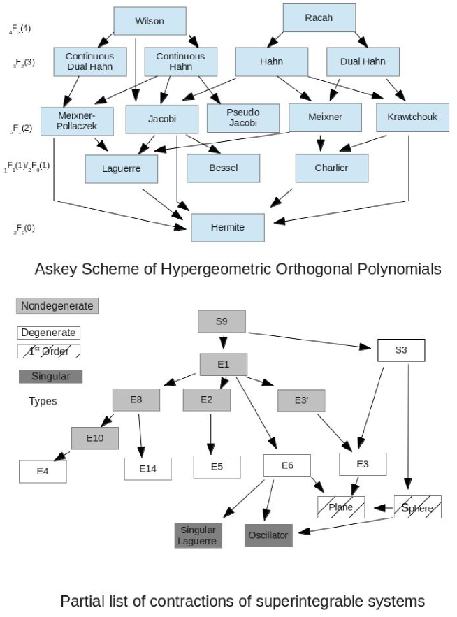
Figure 1: The Askey scheme and contractions of superintegrable systems.

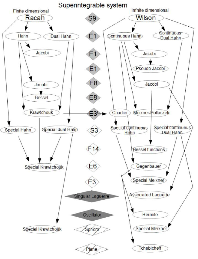
Figure 2: The Askey contraction scheme.

9 The contraction scheme and final comments

The top half of Fig. 1 shows the standard Askey scheme indicating which orthogonal polynomials can be obtained by pointwise limits from other polynomials and, ultimately, from the Wilson or Racah polynomials. The bottom half of Fig. 1 shows how each of the superintegrable systems can be obtained by a series of contractions from the generic system ${\rm S}9$. Not all possible contractions are listed, partly due to complexity and partly to keep the graph from being too cluttered. (For example, all nondegenerate and degenerate superintegrable systems contract to the Euclidean system $H=\partial_{xx}+\partial_{yy}$.) The singular systems are superintegrable in the sense that they have 3 algebraically independent generators, but the coefficient matrix of the 2nd order terms in the Hamiltonian is singular. Fig. 2 shows which orthogonal polynomials are associated with models of which quantum superintegrable system and how contractions enable us to reach all of these functions from ${\rm S}9$. Again not all contractions have been exhibited, but enough to demonstrate that the Askey scheme is a consequence of the contraction structure linking 2nd order quantum superintegrable systems in 2D. It is worth remarking that forthcoming papers by us will simplify considerably the compexity of our approach, [27]. We will show that the structure equations for nondegenerate superintegrable systems can be derived directly from the expression for $R^{2}$ alone, and the structure equations for degenerate superintegrable systems can be derived, up to a multiplicative factor, from the Casimir alone. It will also be demonstrated that all of the contractions of quadratic algebras in the Askey scheme can be induced by natural contractions of the Lie algebras ${\rm e}(2,{\mathbb{C}})$ (6 possible contractions) and ${\rm o}(3,{\mathbb{C}})$ (4 possible contractions).

This method obviously extends to 2nd order systems in more variables. A start on this study can be found in [26]. To extend the method to Askey–Wilson polynomials we would need to find appropriate $q$-quantum mechanical systems with $q$-symmetry algebras and we have not yet been able to do so.

Acknowledgment

This work was partially supported by a grant from the Simons Foundation (# 208754 to Willard Miller, Jr.). The authors would also like to thank the referees for their valuable comments and suggestions.

References

- [1] Andrews G.E., Askey R., Roy R., Special functions, Encyclopedia of Mathematics and its Applications, Vol. 71, Cambridge University Press, Cambridge, 1999.
- [2] Askey R., An integral of Ramanujan and orthogonal polynomials, J. Indian Math. Soc. (N.S.) 51 (1987), 27–36.
- [3] Bonatsos D., Daskaloyannis C., Kokkotas K., Deformed oscillator algebras for two-dimensional quantum superintegrable systems, Phys. Rev. A 50 (1994), 3700–3709, hep-th/9309088.
- [4] Daskaloyannis C., Quadratic Poisson algebras of two-dimensional classical superintegrable systems and quadratic associative algebras of quantum superintegrable systems, J. Math. Phys. 42 (2001), 1100–1119, math-ph/0003017.
- [5] Daskaloyannis C., Tanoudis Y., Quantum superintegrable systems with quadratic integrals on a two dimensional manifold, J. Math. Phys. 48 (2007), 072108, 22 pages, math-ph/0607058.
- [6] Daskaloyannis C., Ypsilantis K., Unified treatment and classification of superintegrable systems with integrals quadratic in momenta on a two-dimensional manifold, J. Math. Phys. 47 (2006), 042904, 38 pages, math-ph/0412055.
- [7] Gao S., Wang Y., Hou B., The classification of Leonard triples of Racah type, Linear Algebra Appl. 439 (2013), 1834–1861.
- [8] Gasper G., Rahman M., Basic hypergeometric series, Encyclopedia of Mathematics and its Applications, Vol. 35, Cambridge University Press, Cambridge, 1990.
- [9] Genest V.X., Vinet L., Zhedanov A., Superintegrability in two dimensions and the Racah–Wilson algebra, arXiv:1307.5539.
- [10] Granovskii Y.I., Lutzenko I.M., Zhedanov A.S., Mutual integrability, quadratic algebras, and dynamical symmetry, Ann. Physics 217 (1992), 1–20.
- [11] Granovskii Y.I., Zhedanov A.S., Lutsenko I.M., Quadratic algebras and dynamics in curved space. I. An oscillator, Theoret. and Math. Phys. 91 (1992), 474–480.
- [12] Granovskii Y.I., Zhedanov A.S., Lutsenko I.M., Quadratic algebras and dynamics in curved space. II. The Kepler problem, Theoret. and Math. Phys. 91 (1992), 604–612.
- [13] Granovskii Y.I., Zhedanov A.S., Lutzenko I.M., Quadratic algebra as a “hidden” symmetry of the Hartmann potential, J. Phys. A: Math. Gen. 24 (1991), 3887–3894.
- [14] Inönü E., Wigner E.P., On the contraction of groups and their representations, Proc. Nat. Acad. Sci. USA 39 (1953), 510–524.
- [15] Izmest’ev A.A., Pogosyan G.S., Sissakian A.N., Winternitz P., Contractions of Lie algebras and separation of variables, J. Phys. A: Math. Gen. 29 (1996), 5949–5962.
- [16] Kalnins E.G., Kress J.M., Miller Jr. W., Second order superintegrable systems in conformally flat spaces. I. 2D classical structure theory, J. Math. Phys. 46 (2005), 053509, 28 pages.
- [17] Kalnins E.G., Kress J.M., Miller Jr. W., Second order superintegrable systems in conformally flat spaces. II. The classical two-dimensional Stäckel transform, J. Math. Phys. 46 (2005), 053510, 15 pages.
- [18] Kalnins E.G., Kress J.M., Miller Jr. W., Nondegenerate 2D complex Euclidean superintegrable systems and algebraic varieties, J. Phys. A: Math. Theor. 40 (2007), 3399–3411, arXiv:0708.3044.
- [19] Kalnins E.G., Kress J.M., Miller Jr. W., Structure relations for the symmetry algebras of quantum superintegrable systems, J. Phys. Conf. Ser. 343 (2012), 012075, 12 pages.
- [20] Kalnins E.G., Kress J.M., Miller Jr. W., Post S., Structure theory for second order 2D superintegrable systems with 1-parameter potentials, SIGMA 5 (2009), 008, 24 pages, arXiv:0901.3081.
- [21] Kalnins E.G., Kress J.M., Miller Jr. W., Winternitz P., Superintegrable systems in Darboux spaces, J. Math. Phys. 44 (2003), 5811–5848, math-ph/0307039.
- [22] Kalnins E.G., Kress J.M., Pogosyan G.S., Miller Jr. W., Completeness of superintegrability in two-dimensional constant-curvature spaces, J. Phys. A: Math. Gen. 34 (2001), 4705–4720, math-ph/0102006.
- [23] Kalnins E.G., Miller Jr. W., Pogosyan G.S., Contractions of Lie algebras: applications to special functions and separation of variables, J. Phys. A: Math. Gen. 32 (1999), 4709–4732.
- [24] Kalnins E.G., Miller Jr. W., Post S., Wilson polynomials and the generic superintegrable system on the 2-sphere, J. Phys. A: Math. Theor. 40 (2007), 11525–11538.
- [25] Kalnins E.G., Miller Jr. W., Post S., Models for the 3D singular isotropic oscillator quadratic algebra, Phys. Atomic Nuclei 73 (2010), 359–366.
- [26] Kalnins E.G., Miller Jr. W., Post S., Two-variable Wilson polynomials and the generic superintegrable system on the 3-sphere, SIGMA 7 (2011), 051, 26 pages, arXiv:1010.3032.
- [27] Kalnins E.G., Miller Jr. W., Subag E., Heinenen R., Contractions of 2nd order superintegrable systems in 2D, in preparation.
- [28] Kalnins E.G., Williams G.C., Miller Jr. W., Pogosyan G.S., On superintegrable symmetry-breaking potentials in -dimensional Euclidean space, J. Phys. A: Math. Gen. 35 (2002), 4755–4773.
- [29] Koekoek R., Lesky P.A., Swarttouw R.F., Hypergeometric orthogonal polynomials and their -analogues, Springer Monographs in Mathematics, Springer-Verlag, Berlin, 2010.
- [30] Koornwinder T.H., Group theoretic interpretations of Askey’s scheme of hypergeometric orthogonal polynomials, in Orthogonal Polynomials and their Applications (Segovia, 1986), Lecture Notes in Math., Vol. 1329, Springer, Berlin, 1988, 46–72.
- [31] Krall H.L., Frink O., A new class of orthogonal polynomials: the Bessel polynomials, Trans. Amer. Math. Soc. 65 (1949), 100–115.
- [32] Kress J.M., Equivalence of superintegrable systems in two dimensions, Phys. Atomic Nuclei 70 (2007), 560–566.
- [33] Létourneau P., Vinet L., Superintegrable systems: polynomial algebras and quasi-exactly solvable Hamiltonians, Ann. Physics 243 (1995), 144–168.
- [34] Miller Jr. W., Symmetry and separation of variables, Encyclopedia of Mathematics and its Applications, Vol. 4, Addison-Wesley Publishing Co., Reading, Mass. – London – Amsterdam, 1977.
- [35] Miller Jr. W., Post S., Winternitz P., Classical and quantum superintegrability with applications, J. Phys. A: Math. Theor., to appear, arXiv:1309.2694.
- [36] Mostafazadeh A., Pseudo-Hermiticity versus symmetry: the necessary condition for the reality of the spectrum of a non-Hermitian Hamiltonian, J. Math. Phys. 43 (2002), 205–214, math-ph/0107001.
- [37] Talman J.D., Special functions: a group theoretic approach (based on lectures by Eugene P. Wigner), W.A. Benjamin, Inc., New York – Amsterdam, 1968.
- [38] Terwilliger P., The universal Askey–Wilson algebra and the equitable presentation of , SIGMA 7 (2011), 099, 26 pages, arXiv:1107.3544.
- [39] Weimar-Woods E., The three-dimensional real Lie algebras and their contractions, J. Math. Phys. 32 (1991), 2028–2033.
- [40] Zhedanov A.S., “Hidden symmetry” of Askey–Wilson polynomials, Theoret. and Math. Phys. 89 (1991), 1146–1157.