A fully-discrete Semi-Lagrangian scheme for a first order mean field game problem

Abstract

In this work we propose a fully-discrete Semi-Lagrangian scheme for a first order mean field game system. We prove that the resulting discretization admits at least one solution and, in the scalar case, we prove a convergence result for the scheme. Numerical simulations and examples are also discussed.

Keywords: Mean field games, First order system, Semi-Lagrangian schemes, Numerical methods.

MSC 2000: Primary, 65M12, 91A13; Secondary, 65M25, 91A23, 49J15, 35F21.

1 Introduction

Initiated by the seminal work of Aumann [7], models to study equilibria in games with a large number of players have become an important research line in the fields of Economics and Applied Mathematics. In this direction, Mean Field Games (MFG) models were recently introduced by J-M. Lasry and P.-L. Lions in [20, 21, 22] in the form of a new system of Partial Differential Equations (PDEs). Under some assumptions, the solution of this system captures the main properties of Nash equilibria for differential games with a very large number of identical “small” players. For a survey of MFG theory and its applications, we refer the reader to [12, 18] and the lectures of P-L. Lions at the Collège de France [24]. The evolutive PDE system introduced in [21], with variables $(v,m)$, is of the form:

$$\begin{array}[]{rl}-\partial_{t}v(x,t)-\sigma^{2}\Delta v(x,t)+H(x,Dv(x,t))&=F(x,m(t)),\;\;\hbox{in }\mathbb{R}^{d}\times(0,T),\\[6.0pt] \partial_{t}m(x,t)-\sigma^{2}\Delta m(x,t)-{\rm{div}}\big{(}\partial_{p}H(x,Dv(x,t))m(x,t)\big{)}&=0,\;\;\;\hbox{in }\mathbb{R}^{d}\times(0,T),\\[6.0pt] v(x,T)=G(x,m(T))\quad\mbox{for }x\in\mathbb{R}^{d}&,\;\;m(0)=m_{0}\in\mathcal{P}_{1},\end{array}$$ (1.1)

where $\sigma\in\mathbb{R}$, $\mathcal{P}_{1}$ denotes the space of probability measures on ${\mathbb{R}^{d}}$ and $F:\mathbb{R}^{d}\times\mathcal{P}_{1}\to\mathbb{R}$, $G:\mathbb{R}^{d}\times\mathcal{P}_{1}\to\mathbb{R}$ and $H:\mathbb{R}^{d}\times\mathbb{R}^{d}\to\mathbb{R}$ are given functions. The Hamiltonian $H$ is supposed to be convex with respect to the second variable $p$. An important feature of the above system is its forward-backward structure: We have a backward Hamilton-Jacobi-Bellman (HJB) equation, i.e. with a terminal condition, coupled with a forward Fokker-Planck equation with initial datum $m_{0}$.

Under rather general assumptions, it can be proved that if $\sigma\neq 0$ then (1.1) admits regular solutions (see [22, Theorem 2.6]). Based on this fact, finite differences schemes have been thoroughly analyzed in the papers [4, 1, 2]. When $H(x,p)$ is quadratic with respect to $p$, specific methods have been proposed in [17, 19].

In this work, we are interested in the numerical analysis of the first order case ($\sigma=0$) with quadratic Hamiltonian $H(x,p)=\mbox{$\frac{1}{2}$}|p|^{2}$. In this case, system (1.1) takes the form

$$\begin{array}[]{rcl}-\partial_{t}v(x,t)+\mbox{$\frac{1}{2}$}|Dv(x,t)|^{2}&=&F(x,m(t)),\hskip 5.69046pt\hbox{in }\mathbb{R}^{d}\times(0,T),\\[6.0pt] \partial_{t}m(x,t)-{\rm{div}}\big{(}Dv(x,t)m(x,t)\big{)}&=&0,\quad\hbox{in }\mathbb{R}^{d}\times(0,T),\\[6.0pt] v(x,T)=G(x,m(T))\quad\mbox{for }x\in\mathbb{R}^{d}&,&m(0)=m_{0}\in\mathcal{P}_{1}.\end{array}$$ (1.2)

The second equation (i.e. the Fokker-Planck equation with $\sigma=0$) is called the continuity equation and describes the transport of the initial measure $m_{0}$ by the flow induced by $-Dv(\cdot,\cdot)$. When $F$ and $G$ are non-local and regularizing operators (see [22]), the existence of a solution $(v,m)$ of (1.2) can be proved by a fixed point argument (see [12, 24]). However, the numerical approximation of $(v,m)$ is very challenging since, besides the forward-backward structure of (1.2), we can expect only Lipchitz regularity for $v$ and $L^{\infty}$ regularity for $m$ (see e.g. [12]).

Although several numerical methods have been analyzed for each one of the equations in (1.2) (see e.g. the monographs [15, 29, 25] and the references therein for the HJB equation and [26, 30] for the continuity equation), when the coupling between both equations is present, the authors are aware only of references [16], for the scalar case $d=1$, and [3], for the multidimensional case. However, in both references the structure of the system is forward-forward, i.e. both equations have initial conditions. This fact completely changes the theoretical and numerical analysis of the problem. As a matter of fact, for example in [3], the key property for convergence result of the proposed numerical scheme is a one side Lipschitz condition for $Dv(\cdot,\cdot)$ of the form:

$$\exists C>0\;\;\mbox{such that }\forall t\in[0,T],\;\;\langle Dv(x,t)-Dv(y,t),x-y\rangle\geq-C|x-y|^{2}.$$ (1.3)

By the results in [27], condition (1.3) assures the stability of the so-called Fillipov characteristics and of the associated measure solutions of the continuity equation, which are the key to obtain their convergence result. Unfortunately, in our case (1.3) corresponds to the semiconvexity of $v$, which does not holds for an arbitrary time horizon $T$ (see [11]).

Our line of research follows the ideas in [10], where a semi-discrete in time Semi-Lagrangian scheme is proposed to approximate (1.2) and a convergence result is obtained. However, since the space variable is not discretized, the resulting scheme cannot be simulated. In this paper we propose a fully-discrete Semi-Lagrangian scheme for (1.2) and we study its main properties. We prove that the fully-discrete problem admits at least one solution and, for the case $d=1$, we are able to prove the convergence of the scheme to a solution $(v,m)$ of (1.2), when the discretization parameters tend to zero in a suitable manner. The key point of the proof is a discrete semiconcavity property for the discretized solutions. Let us point out that our approximation scheme is presented in a general dimension $d$ and several properties are proved in this generality. However, since in general (1.3) does not hold, uniform estimates in the $L^{\infty}$ norm for the solutions of the scheme seems to be unavoidable in order to prove the convergence (see [12] for similar arguments regarding the vanishing viscosity approximation of (1.2)). Since we are able to prove these bounds only for $d=1$, our convergence result for the fully-discrete scheme is valid only in this case.

The paper is organized as follows: In Section 2 we state our main assumptions, we collect some useful properties about semiconcave functions and we recall the main existence and uniqueness results for (1.2). Section 3 is devoted to the fully-discrete scheme. We establish the main properties of the scheme and we prove our main results: The fully-discrete scheme admits at least one solution and, if $d=1$ and the discretization parameters tend to zero in a suitable manner, every limit point of the solutions of the scheme is a solution of (1.2). Finally, in Section 4 we display some numerical simulations in the case of one space dimension.

2 Preliminaries

2.1 Basic assumptions and existence and uniqueness results for (1.2)

We denote by $\mathcal{P}_{1}$ the set of the probability measures $m$ such that $\int_{\mathbb{R}^{d}}|x|dm(x)<\infty$. The set $\mathcal{P}_{1}$ is be endowed with the Kantorovich-Rubinstein distance

$$\mathbf{d}_{1}(\mu,\nu)=\sup\left\{\int_{\mathbb{R}^{d}}\phi(x){\rm d}[\mu-\nu](x)\ ;\ \phi:\mathbb{R}^{d}\to\mathbb{R}\hskip 8.5359pt\mbox{is 1-Lipschitz}\right\}.$$ (2.1)

Given a measure $\mu\in\mathcal{P}_{1}$ we denote by $\mathrm{supp}\;(\mu)$ its support. In what follows, in order to simplify the notation, the operator $D$ (resp. $D^{2}$) will denote the derivative (resp. the second derivative) with respect to the space variable $x\in\mathbb{R}^{d}$. We suppose that the functions $F,G:\mathbb{R}^{d}\times\mathcal{P}_{1}\to\mathbb{R}$ and the measure $m_{0}$, which are the data of (1.2), satisfy the following assumptions:
(H1) $F$ and $G$ are continuous over $\mathbb{R}^{d}\times\mathcal{P}_{1}$.
(H2) There exists a constant $c_{0}>0$ such that for any $m\in\mathcal{P}_{1}$

$$\|F(\cdot,m)\|_{C^{2}}+\|G(\cdot,m)\|_{C^{2}}\leq c_{0},$$

where $\|f(\cdot)\|_{C^{2}}:=\sup_{x\in\mathbb{R}^{d}}\{|f(x)|+|Df(x)|+|D^{2}f(x)|\}.$
(H3) The initial condition $m_{0}\in\mathcal{P}_{1}$ is absolutely continuous with respect to the Lebesgue measure, with density still denoted by $m_{0}$, and satisfies $\mathrm{supp}\;(m_{0})\subset B(0,c_{1})$ and $\|m_{0}\|_{\infty}\leq c_{1}$, for some $c_{1}>0$ .

As a general rule in this paper, given an absolutely continuous measure (w.r.t the Lebesgue measure in $\mathbb{R}^{d}$) $m\in\mathcal{P}_{1}$, its density will still be denoted by $m$. Let us recall the definition of a solution $(v,m)$ of (1.2) (see [21, 22]).

Definition 2.1

The pair $(v,m)\in W^{1,\infty}_{loc}(\mathbb{R}^{d}\times[0,T])\times L^{1}(\mathbb{R}^{d}\times(0,T))$ is a solution of (1.2) if the first equation is satisfied in the viscosity sense, while the second one is satisfied in the distributional sense. More precisely, for every $\phi\in\mathcal{C}_{c}^{\infty}\left((\mathbb{R}^{d}\times[0,T)\right)$

$$\int_{\mathbb{R}^{d}}\phi(x,0)m_{0}(x){\rm d}x+\int_{0}^{T}\int_{\mathbb{R}^{d}}\left[\partial_{t}\phi(x,t)-\langle Dv(x,t),D\phi(x,t)\rangle\right]m(x,t){\rm d}x{\rm d}t=0.$$ (2.2)

Remark 2.1

Classical arguments (see e.g. [5]) imply that (2.2) is equivalent to

$$\int_{\mathbb{R}^{d}}\phi(x)m_{0}(x){\rm d}x-\int_{0}^{t}\int_{\mathbb{R}^{d}}\langle Dv(x,s),D\phi(x)\rangle m(x,s){\rm d}x{\rm d}s=0,$$ (2.3)

for all $t\in[0,T]$ and $\phi\in C_{c}^{\infty}(\mathbb{R}^{d})$.

The following existence result is proved in [24, 12].

Theorem 2.1

Under (H1)-(H3) there exists at least a solution $(v,m)$ of (1.2).

A uniqueness result can be obtained assuming
(H4) The following monotonicity conditions hold true

$$\begin{array}[]{l}\int_{\mathbb{R}^{d}}\left[F(x,m_{1})-F(x,m_{2})\right]{\rm d}[m_{1}-m_{2}](x)\geq 0\quad\mbox{for all }\ m_{1},m_{2}\in\mathcal{P}_{1}\\[6.0pt] \int_{\mathbb{R}^{d}}\left[G(x,m_{1})-G(x,m_{2})\right]{\rm d}[m_{1}-m_{2}](x)\geq 0\quad\mbox{for all }\,m_{1},m_{2}\in\mathcal{P}_{1}.\end{array}$$ (2.4)

We have (see [24, 12]):

Theorem 2.2

Under (H1)-(H4) system (1.2) admits a unique solution $(v,m)$.

2.2 Standard semiconcavity results

In the proof of Theorem 2.1, as well as in the the proof of our main results, the concept of semiconcavity plays a crucial role. For a complete account of the theory and its applications to the solution of HJB equations, we refer the reader to the book [11].

Definition 2.2

We say that $w:\mathbb{R}^{d}\to\mathbb{R}$ is semiconcave with constant $C_{conc}>0$ if for every $x_{1},x_{2}\in\mathbb{R}^{d}$, $\lambda\in(0,1)$ we have

$$w(\lambda x_{1}+(1-\lambda)x_{2})\geq\lambda w(x_{1})+(1-\lambda)w(x_{2})-\lambda(1-\lambda)\frac{C_{conc}}{2}|x_{1}-x_{2}|^{2}.$$ (2.5)

A function $w$ is said to be semiconvex if $-w$ is semiconcave.

Recall that for $w:\mathbb{R}^{d}\to\mathbb{R}$ the super-differential $D^{+}w(x)$ at $x\in\mathbb{R}^{d}$ is defined as

$$D^{+}w(x):=\left\{p\in\mathbb{R}^{d}\ ;\ \limsup_{y\to x}\frac{w(y)-w(x)-\langle p,y-x\rangle}{|y-x|}\leq 0\right\}.$$ (2.6)

We collect in the following Lemmas some useful properties of semiconcave functions (see [11]).

Lemma 2.1

For a function $w:\mathbb{R}^{d}\to\mathbb{R}$, the following assertions are equivalent:
(i) The function $w$ is semiconcave, with constant $C_{conc}$.
(ii) For all $x,y\in\mathbb{R}^{d}$, we have

$$w(x+y)+w(x-y)-2w(x)\leq C_{conc}|y|^{2}.$$

(iii) For all $x$, $y\in\mathbb{R}^{d}$ and $p\in D^{+}w(x)$, $q\in D^{+}w(y)$

$$\langle q-p,y-x\rangle\leq C_{conc}|x-y|^{2}.$$ (2.7)

(iv) Setting $I_{d}$ for the identity matrix, we have that $D^{2}w\leq C_{conc}I_{d}$ in the sense of distributions.

Lemma 2.2

Let $w:\mathbb{R}^{d}\to\mathbb{R}$ be semiconcave. Then:
(i) $w$ is locally Lipschitz.
(ii) If $w_{n}$ is a sequence of semiconcave functions (with the same semiconcavity constant) converging pointwise to $w$, then the convergence is locally uniform and $Dw_{n}(\cdot)\to Dw(\cdot)$ a.e. in $\mathbb{R}^{d}$.

2.3 Representation formulas for the solutions of the HJB and the continuity equations

Let $\mu\in C([0,T];\mathcal{P}_{1})$ be given and let us denote by $v[\mu]$ for the unique viscosity solution of

$$\left.\begin{array}[]{rcl}-\partial_{t}v(x,t)+\mbox{$\frac{1}{2}$}|Dv(x,t)|^{2}&=&F(x,\mu(t)),\hskip 5.69046pt\hbox{in }\mathbb{R}^{d}\times(0,T),\\[6.0pt] v(x,T)&=&G(x,\mu(T))\hskip 8.5359pt\hbox{in }\mathbb{R}^{d}.\end{array}\right\}$$ (2.8)

Under assumptions (H1)-(H2), standard results (see e.g. [8]) yield that for each $(x,t)\in\mathbb{R}^{d}\times[0,T]$, the following representation formula for $v[\mu](x,t)$ holds true

$$\left.\begin{array}[]{l}v[\mu](x,t)=\displaystyle\mbox{inf}_{\alpha\in L^{2}([t,T];\mathbb{R}^{d})}\int_{t}^{T}\left[\mbox{$\frac{1}{2}$}|\alpha(s)|^{2}+F(X^{x,t}[\alpha](s),\mu(s))\right]{\rm d}s\\[8.0pt] \hskip 113.81102pt+G(X^{x,t}[\alpha](T),\mu(T)),\\[6.0pt] \mbox{where }\hskip 39.83368ptX^{x,t}[\alpha](s):=x-\int_{t}^{s}\alpha(r){\rm d}r\hskip 14.22636pt\mbox{for all }s\in[t,T].\end{array}\right\}$$

We set $\mathcal{A}^{x,t}[\mu]$ for the set of optimal controls $\alpha$ of $(\mathcal{CP})^{x,t}[\mu]$, i.e. for the set of solutions of $(\mathcal{CP})^{x,t}[\mu]$. Classical arguments imply that for all $(x,t)$ the set $\mathcal{A}^{x,t}[\mu]$ is non empty.

We now collect some important well known properties of problem $(\mathcal{CP})^{x,t}[\mu]$ (see e.g. [11, 12]).

Proposition 2.1

Under (H1)-(H2), The value function $v[\mu]$ satisfies the following properties:
(i) We have that $(x,t)\to v[\mu](x,t)$ is Lipchitz, with a Lipschitz constant independent of $\mu$.
(ii) For all $t\in[0,T]$ the function $v[\mu](\cdot,t)\in\mathbb{R}$ is semiconcave, uniformly with respect to $\mu$.
(iii) There exists a constant $c_{2}>0$ (independent of $(\mu,x,t)$) such that

$$\|\alpha\|_{L^{\infty}([t,T];\mathbb{R}^{d})}\leq c_{2}\hskip 8.5359pt\mbox{for all }\ \alpha\in\mathcal{A}^{x,t}[\mu].$$

(iv) For all $(x,t)$ and $\alpha\in\mathcal{A}^{x,t}[\mu]$, we have that

$$\alpha(t)\in D^{+}v[\mu](x,t).$$ (2.9)

(v) For all $t\in[0,T]$ the function $v[\mu](\cdot,t)$ is differentiable at $x$ iff there exists $\alpha\in\mathcal{A}^{x,t}[\mu]$ such that $\mathcal{A}^{x,t}[\mu]=\{\alpha\}$. In this case, we have that

$$Dv[\mu](x,t)=\alpha(t).$$ (2.10)

(vi) For every $s\in(t,T]$ and $\alpha\in\mathcal{A}^{x,t}[\mu]$, we have that $v[\mu](\cdot,\cdot)$ is differentiable at $(X^{x,t}[\alpha](s),s)$.

Now, we define a measurable selection of optimal flows, i.e. of optimal trajectories for the family of problems $\{(\mathcal{CP})^{x,t}[\mu]\;;\;(x,t)\in\mathbb{R}^{d}\times[0,T]\}$. Classical arguments (see [12, 6]) show that the multivalued map $(x,t)\to\mathcal{A}^{x,t}[\mu]$, admits a measurable selection $\alpha^{x,t}[\mu](\cdot)$. Given $(x,t)$ the flow $\Phi[\mu](x,t,\cdot)$ is defined as

$$\Phi[\mu](x,t,s):=x-\int_{t}^{s}\alpha^{x,t}[\mu](r){\rm d}r\hskip 11.38092pt\mbox{for all }s\in[t,T].$$ (2.11)

By Proposition 2.1(v)-(vi), omitting the dependence on $\mu$ for notational convenience, $\Phi(x,t,\cdot)$ satisfies

$$\left.\begin{array}[]{rcl}\frac{\partial}{\partial s}\Phi(x,t,s)&=&-Dv[\mu](\Phi(x,t,s),s)\hskip 11.38092pt\mbox{for }s\in(t,T),\\[6.0pt] \Phi(x,t,t)&=&x.\end{array}\right\}$$ (2.12)

For all $t\in[0,T]$, let us define $m[\mu](t)$ as the initial measure $m_{0}$ transported by the flow $\Phi[\mu]$. More precisely,

$$m[\mu](t):=\Phi[\mu](\cdot,0,t)\sharp m_{0},$$ (2.13)

i.e.

$$m[\mu](t)(A)=m_{0}\left(\Phi[\mu]^{-1}(\cdot,0,t)(A)\right)\hskip 8.5359pt\mbox{for all }A\in\mathcal{B}(\mathbb{R}^{d}),$$

or equivalently, for all bounded and continuous $\phi:\mathbb{R}^{d}\to\mathbb{R}$,

$$\int_{\mathbb{R}^{d}}\phi(x){\rm d}\left[m[\mu](t)\right](x)=\int_{\mathbb{R}^{d}}\phi\left(\Phi[\mu](x,0,t)\right){\rm d}m_{0}(x).$$

Since $\Phi[\mu](x,\cdot,\cdot)$ satisfies the semigroup property, omitting the dependence on $\mu$ for simplicity,

$$\Phi(x,s,t)=\Phi(\Phi(x,s,r),r,t)\hskip 11.38092pt\mbox{for all }r\in[s,t],$$

we easily check that

$$m[\mu](t):=\Phi(\cdot,r,t)\sharp\left[\Phi(\cdot,0,r)\sharp m_{0}\right]=\Phi(\cdot,r,t)\sharp\left[m[\mu](r)\right]\hskip 11.38092pt\mbox{for all }r\in[s,t].$$ (2.14)

The fundamental result is the following

Proposition 2.2

There exists a constant $c_{3}>0$ (independent of $(\mu,x,y,r,t)$), such that

$$|\Phi(x,r,t)-\Phi(y,r,t)|\geq c_{3}|x-y|\hskip 8.5359pt\mbox{ {\rm for all} }\hskip 8.5359pt0\leq r\leq t,\hskip 8.5359pt\mbox{{\rm and} }\hskip 8.5359ptx,y\in\mathbb{R}^{d}.$$

The key in the proof of the above Proposition (see e.g. [12, Lemma 4.13]) is the semiconcavity of $v[\mu](\cdot,t)$, which is uniform w.r.t $\mu$, and Gronwall’s Lemma. As a consequence we have that (see e.g. [12, Theorem 4.18 and Lemma 4.14])

Theorem 2.3

We have that $m[\mu](\cdot)$ is the unique solution (in the distributional sense) of

$$\left.\begin{array}[]{rcl}\partial_{t}m(x,t)-{\rm{div}}\big{(}Dv[\mu](x,t)m(x,t)\big{)}&=&0,\quad\hbox{in }\mathbb{R}^{d}\times(0,T),\\[6.0pt] m(x,0)&=&m_{0}(x)\hskip 8.5359pt\hbox{in }\mathbb{R}^{d}.\end{array}\right\}$$ (2.15)

Moreover, there exists a constant $c_{4}>0$, independent of $\mu$, such that $m[\mu]$ satisfies the following properties:
(i) For all $t\in[0,T]$, the measure $m[\mu](t)$ is absolutely continuous (with density still denoted by $m[\mu](t)$), has a support in $B(0,c_{4})$ and $\|m[\mu](t)\|_{\infty}\leq c_{4}$.
(ii) For all $t,t^{\prime}\in[0,T]$, we have that

$$\mathbf{d}_{1}(\mu(t),\mu(t^{\prime}))\leq c_{4}|t-t^{\prime}|.$$

Remark 2.2

In the proof of the above result (see [12]) Proposition 2.2 is crucial in order to show that the transported measure $m[\mu](\cdot)$ is absolutely continuous, as $m_{0}$, and its density remains uniformly bounded in $L^{\infty}(\mathbb{R}^{d})$.

Theorem 2.3 (i)-(ii) implies that $m[\mu](\cdot)\in C([0,T];\mathcal{P}_{1})$. We thus see that (1.2) is equivalent to find $m\in C([0,T];\mathcal{P}_{1})$, such that

$$m(t)=\Phi[m](\cdot,0,t)\sharp m_{0}\hskip 14.22636pt\mbox{for all }t\in[0,T].$$

3 The fully-discrete scheme

Given $h,\rho>0$, we consider a $d$ dimensional lattice $\mathcal{G}_{\rho}:=\{x_{i}=i\rho,\;i\in\mathbb{Z}^{d}\}$ and a time-space grid $\mathcal{G}_{\rho,h}:=\mathcal{G}_{\rho}\times\{t_{k}\}_{k=0}^{N}$, where $t_{k}=kh$ ($k=0,\ldots,N$) and $t_{N}=Nh=T$. We set $B(\mathcal{G}_{\rho})$ and $B(\mathcal{G}_{\rho,h})$ for the space of bounded functions defined on $\mathcal{G}_{\rho}$ and $\mathcal{G}_{\rho,h}$, respectively. Given $f\in B(\mathcal{G}_{\rho})$ and $g\in B(\mathcal{G}_{\rho,h})$ we will use the notation

$$f_{i}:=f(x_{i}),\;\;\hskip 11.38092ptg_{i,k}:=g(x_{i},t_{k})\hskip 11.38092pt\mbox{for all $i\in\mathbb{Z}^{d}$ and $k=0,\ldots,N$}.$$

Let us consider the $\mathbb{P}_{1}$ basis $\{\beta_{i}\;;\;i\in\mathbb{Z}^{d}\}$, where the function $\beta_{i}:\mathbb{R}^{d}\to\mathbb{R}$ is defined by $\beta_{i}(x):=\big{[}1-\frac{\|x-x_{i}\|_{1}}{\rho}\big{]}_{+}:=\max\{1-\frac{\|x-x_{i}\|_{1}}{\rho},0\}$. Denoting by $e_{1},\ldots,e_{d}$ the canonical base of $\mathbb{R}^{d}$, it is easy to verify that $\beta_{i}(x)$ is continuous with compact support contained in $Q(x_{i}):=[x_{i}-\rho e_{1},x_{i}+\rho e_{1}]\times\dots\times[x_{i}-\rho e_{d},x_{i}+\rho e_{d}]$, $0\leq\beta_{i}\leq 1$, $\beta_{i}(x_{j})=\delta_{ij}$ (the Kronecker symbol) and $\sum_{i\in\mathbb{Z}^{d}}\beta_{i}(x)=1$. Let us consider the interpolation operator $I[\cdot]:B(\mathcal{G}_{\rho})\to C_{b}(\mathbb{R}^{d})$, defined by

$$I[f](\cdot):=\sum_{i\in\mathbb{Z}^{d}}f_{i}\beta_{i}(\cdot).$$ (3.1)

We recall a standard estimate for $I$ (see e.g. [14, 28]). Given $\phi\in C_{b}(\mathbb{R}^{d})$, let us define $\hat{\phi}\in B(\mathcal{G}_{\rho})$ by $\hat{\phi}_{i}:=\phi(x_{i})$ for all $i\in\mathbb{Z}^{d}$. We have that

$$\sup_{x\in\mathbb{R}^{d}}|I[\hat{\phi}](x)-\phi(x)|=O(\rho^{\gamma}),$$ (3.2)

where $\gamma=1$ if $\phi$ is Lipschitz and $\gamma=2$ if $\phi\in C^{2}(\mathbb{R}^{d})$ with bounded first and second derivatives.

3.1 The fully-discrete scheme for the HJB equation

For a given $\mu\in C([0,T],\mathcal{P}_{1})$, we define recursively $v\in B(\mathcal{G}_{\rho,h})$ using the following Semi-Lagrangian scheme for (2.8):

$$v_{i,k}=S_{\rho,h}[\mu](v_{\cdot,k+1},i,k)\quad k=0,\ldots,N-1\hskip 8.5359pt\mbox{and }\hskip 5.69046ptv_{i,N}=G(x_{i},\mu(t_{N})),\\$$ (3.3)

where $S_{\rho,h}[\mu]:B(\mathcal{G}_{\rho})\times\mathbb{Z}^{d}\times\{0,\ldots,N-1\}\to\mathbb{R}$ is defined as

$$S_{\rho,h}[\mu](f,i,k):=\inf_{\alpha\in\mathbb{R}^{d}}\left[I[f](x_{i}-h\alpha)+\mbox{$\frac{1}{2}$}h|\alpha|^{2}\right]+hF(x_{i},\mu(t_{k})).$$ (3.4)

The following properties of $S_{\rho,h}[\mu]$ are a straightforward consequence of the definition and assumptions (H1) and (H2).

Lemma 3.1

The following assertions hold true:
(i) [The scheme is well defined] There exists at least one $\alpha\in\mathbb{R}^{d}$ that minimizes the r.h.s. of (3.4). Moreover, there exists $c_{5}>0$ such that $\sup_{i\in\mathbb{Z}^{d},k=0,\ldots,N}|v_{i,k}|\leq c_{5}$.
(ii)[Monotonicity] For all $v,w\in B(\mathcal{G}_{\rho})$ with $v\leq w$, we have that

$$S_{\rho,h}[\mu](v,i,k)\leq S_{\rho,h}[\mu](w,i,k)\hskip 14.22636pt\forall\;i\in\mathbb{Z}^{d},\;k=0,\ldots,N.$$ (3.5)

(iii) For every $K\in\mathbb{R}$ and $w\in B(\mathcal{G}_{\rho})$ we have

$$S_{\rho,h}[\mu](w+K,i,n)=S_{\rho,h}[\mu](w,i,n)+K.$$ (3.6)

(iv)[Consistency] Let $(\rho_{n},h_{n})\to 0$ (as $n\uparrow\infty$) and consider a sequence of grid points $(x_{i_{n}},t_{k_{n}})\to(x,t)$ and a sequence $\mu_{n}\in C([0,T];\mathcal{P}_{1})$ such that $\mu_{n}\to\mu$. Then, for every $\phi\in C^{1}\left(\mathbb{R}^{d}\times[0,T)\right)$, we have

$$\begin{array}[]{ll}\lim_{n\to\infty}\frac{1}{h_{n}}\left[\phi(x_{i_{n}},t_{k_{n}})-S_{\rho_{n},h_{n}}[\mu_{n}](\phi_{k_{n+1}},i_{n},k_{n})\right]&=-\partial_{t}\phi(x,t)+\frac{1}{2}|D\phi(x,t)(x,t)|^{2}\\ &\;\hskip 7.11317pt-F(x,\mu(t)).\end{array}$$ (3.7)

where $\phi_{k}=\{\phi(x_{i},t_{k})\}_{i\in\mathbb{Z}^{d}}$.

We define

$$v_{\rho,h}[\mu](x,t):=I[v_{\cdot,\left[\frac{t}{h}\right]}](x)\hskip 14.22636pt\mbox{for all }\hskip 5.69046pt(x,t)\in\mathbb{R}^{d}\times[0,T],$$ (3.8)

where we recall that $v_{i,k}$ is defined by (3.3).

Lemma 3.2

For every $t\in[0,T]$, the following assertions hold true:
(i) [Lipschitz property] The function $v_{\rho,h}[\mu](\cdot,t)$ is Lipschitz with constant independent of $(\rho,h,\mu,t)$.
(ii) [Weak semiconcavity] There exists $c_{6}>0$ independent of $(\rho,h,\mu,t)$ such that for all $x$,$y\in\mathbb{R}^{d}$ we have

$$v_{\rho,h}[\mu](x+y,t)-2v_{\rho,h}[\mu](x,t)+v_{\rho,h}[\mu](x-y,t)\leq c_{6}\left[|y|^{2}+\rho^{2}(E(x+y)+E(x-y))\right],$$ (3.9)

where $E:\mathbb{R}^{d}\to\mathbb{R}$ is a nonnegative, continuous and bounded function vanishing in $\mathcal{G}_{\rho}$.

Proof. By (H2) we have that $\|DG(\cdot,\mu(T))\|_{\infty}\leq c_{0}$ and so $I[G](\cdot,\mu(T))$ is $c_{0}$-Lipschitz. Thus, by the (3.3) and (3.8), we get that $v_{\rho,h}[\mu](\cdot,t_{N-1})$ is Lipschitz with constant $hc_{0}+c_{0}$. Iterating the argument, using (H2) for $F$, we get that $v_{\rho,h}[\mu](\cdot,t)$ is $c_{0}(1+T)$ Lipschitz for all $t\in[0,T]$. The proof of the second assertion is provided e.g. in [3, Lemma 4.1].   

Remark 3.1

Inequality (3.9) is a consequence of a discrete-semiconcavity property of $v_{i,k}$ (see e.g. [23]).

Theorem 3.1

Let $(\rho_{n},h_{n})\to 0$ (as $n\uparrow\infty$) be such that $\frac{\rho_{n}^{2}}{h_{n}}\to 0$. Then, for every sequence $\mu_{n}\in C([0,T];\mathcal{P}_{1})$ such that $\mu_{n}\to\mu$ in $C([0,T];\mathcal{P}_{1})$, we have that $v_{\rho_{n},h_{n}}[\mu_{n}]\to v[\mu]$ uniformly over compact sets.

Proof. Using assumption (H1), the proof is a straightforward variation of the one in [13], which is a revised proof of the result given in [9]. However, for the sake of completeness we provide the details. For $(y,s)\in\mathbb{R}^{d}\times[0,T]$, set

$$v^{*}(y,s):=\underset{n\to\infty}{\limsup_{(y^{\prime},s^{\prime})\to(y,s)}}v_{\rho_{n},h_{n}}[\mu_{n}](y^{\prime},s^{\prime}),\hskip 14.22636ptv_{*}(y,s):=\underset{n\to\infty}{\liminf_{(y^{\prime},s^{\prime})\to(y,s)}}v_{\rho_{n},h_{n}}[\mu_{n}](y^{\prime},s^{\prime}).$$

Let us prove that $v^{*}$ is a viscosity subsolution of

$$\begin{array}[]{rcl}-\partial_{t}v(x,t)+\mbox{$\frac{1}{2}$}|Dv(x,t)|^{2}&=&F(x,\mu(t))\quad\mbox{for }(x,t)\in\mathbb{R}^{d}\times(0,T),\\[6.0pt] v(x,T)&=&G(x,\mu(T))\quad\mbox{for }x\in\mathbb{R}^{d}.\end{array}$$ (3.10)

Let $(\bar{y},\bar{s})\in\mathbb{R}^{d}\times(0,T)$ and $\phi\in C^{1}(\mathbb{R}^{d}\times(0,T))$ be such that $v^{*}(\bar{y},\bar{s})=\phi(\bar{y},\bar{s})$ and $v^{*}-\phi$ has a global strict maximum at $(\bar{y},\bar{s})$. Since $v^{*}(\cdot,\cdot)$ is upper semicontinuous, a standard argument in the theory of viscosity solutions implies that, up to some subsequence, there exists $(y_{n},s_{n})\to(\bar{y},\bar{s})$, such that

$$(v_{\rho_{n},h_{n}}[\mu_{n}]-\phi)(y_{n},s_{n})=\max_{(y,s)\in\mathbb{R}^{d}\times(0,T)}(v_{\rho_{n},h_{n}}[\mu_{n}]-\phi)(y,s)$$

$$\hskip 8.5359pt\mbox{and }\hskip 5.69046pt(v_{\rho_{n},h_{n}}[\mu_{n}]-\phi)(y_{n},s_{n})\to(v^{*}-\phi)(\bar{y},\bar{s})=0.$$

Thus, for any $(y,s)\in\mathbb{R}^{d}\times[0,T]$ we have that

$$v_{\rho_{n},h_{n}}[\mu_{n}](y,s)\leq\phi(y,s)+\xi_{n},\hskip 11.38092pt\mbox{with }\hskip 11.38092pt\xi_{n}:=(v_{\rho_{n},h_{n}}[\mu_{n}]-\phi)(y_{n},s_{n})\to 0.$$ (3.11)

Let $k:=\mathbb{N}\to\{0,\ldots,N-1\}$ be such that $s_{n}\in[t_{k(n)},t_{k(n)+1})$. Evidently, we have that $t_{k(n)}\to\bar{s}$. By taking $y=x_{i}$, $i\in\mathbb{Z}^{d}$, and $s=t_{k(n)+1}$ in (3.11), we get that

$$v_{i,k(n)+1}\leq\phi(x_{i},t_{k(n)+1})+\xi_{n}\hskip 11.38092pt\mbox{for all }i\in\mathbb{Z}^{d}.$$ (3.12)

Lemma 3.1(ii)-(iii) implies that

$$S_{\rho_{n},h_{n}}[\mu_{n}](v_{\cdot,k(n)+1},i,k(n))\leq S_{\rho_{n},h_{n}}[\mu_{n}](\phi_{k(n)+1},i,k(n))+\xi_{n}\hskip 11.38092pt\mbox{for all }i\in\mathbb{Z}^{d}.$$

In particular, using (3.3), we get

$$v_{i,k(n)}\leq S_{\rho_{n},h_{n}}[\mu_{n}](\phi_{k(n)+1},i,k(n))+\xi_{n}\hskip 11.38092pt\mbox{for all }i\in\mathbb{Z}^{d},$$

which yields, by the definition of $v_{\rho_{n},h_{n}}[\mu_{n}](y_{n},s_{n})$ in (3.8),

$$v_{\rho_{n},h_{n}}[\mu_{n}](y_{n},s_{n})\leq\sum_{i\in\mathbb{Z}^{d}}\beta_{i}(y_{n})S_{\rho_{n},h_{n}}[\mu_{n}](\phi_{k(n)+1},i,k(n))+\xi_{n}.$$

Now, recalling the definition of $\xi_{n}$, we get

$$\phi(y_{n},s_{n})\leq\sum_{i\in\mathbb{Z}^{d}}\beta_{i}(y_{n})S_{\rho_{n},h_{n}}[\mu_{n}](\phi_{k(n)+1},i,k(n)).$$ (3.13)

We claim now that $\phi(y_{n},s_{n})=\phi(y_{n},t_{k(n)})+O(h_{n}^{2})$. In fact, either $s_{n}=t_{k(n)}$ (and the claim obviously holds), or $s_{n}\in(t_{k(n)},t_{k(n)+1})$. In the latter case, since $(v_{\rho_{n},h_{n}}-\phi)(y_{n},\cdot)$ has a maximum at $s_{n}$ and $v_{\rho_{n},h_{n}}$ is constant in $(t_{k(n)},t_{k(n)+1})$, then $\partial_{t}\phi(y_{n},s_{n})=0$ and the claim follows from a Taylor expansion. Thus, by our claim and (3.13), we have that

$$\phi(y_{n},t_{k(n)})\leq\sum_{i\in\mathbb{Z}^{d}}\beta_{i}(y_{n})S_{\rho_{n},h_{n}}[\mu_{n}](\phi_{k(n)+1},i,k(n))+o(h_{n}).$$ (3.14)

Now, inequality (3.14), estimate (3.2) and the fact that $\rho_{n}^{2}/h_{n}\to 0$ imply that

$$\lim_{n\to\infty}\sum_{i\in\mathbb{Z}^{d}}\beta_{i}(y_{n})\frac{\phi(x_{i},t_{k(n)})-S_{\rho_{n},h_{n}}[\mu_{n}](\phi_{k(n)+1},i,k(n))}{h_{n}}\leq 0.$$

Finally, by the consistency property in Lemma 3.1(iv) we obtain that

$$-\partial_{t}\phi(\bar{y},\bar{s})+\frac{1}{2}|D\phi(\bar{y},\bar{s})|^{2}-F(\bar{y},\mu(\bar{s}))\leq 0,$$

which implies that $v^{*}$ is a subsolution of (3.11). The supersolution property for $v_{*}$ can be proved in a similar manner. Therefore, by a classical comparison argument, $v_{\rho_{n},h_{n}}[\mu_{n}]$ converges locally uniformly to $v[\mu]$ in $\mathbb{R}^{d}\times(0,T)$.   

Let $\rho\in C^{\infty}_{c}(\mathbb{R}^{d})$ with $\rho\geq 0$ and $\int_{\mathbb{R}^{d}}\rho(x){\rm d}x=1$. For $\varepsilon>0$, we consider the mollifier $\rho_{\varepsilon}(x):=\frac{1}{\varepsilon^{d}}\rho\left(\frac{x}{\varepsilon}\right)$ and define

$$v^{\varepsilon}_{\rho,h}[\mu](\cdot,t):=\rho_{\varepsilon}\ast v_{\rho,h}[\mu](\cdot,t)\hskip 14.22636pt\mbox{for all }\hskip 5.69046ptt\in[0,T].$$ (3.15)

Using Lemma 3.2(i) we easily check the estimates

$$\begin{array}[]{rcl}\|v^{\varepsilon}_{\rho,h}[\mu](\cdot,\cdot)-v_{\rho,h}[\mu](\cdot,\cdot)\|_{\infty}&=&\gamma\varepsilon,\\[6.0pt] \|D^{\alpha}v^{\varepsilon}_{\rho,h}[\mu](\cdot,\cdot)\|_{\infty}&=&c_{\alpha}\varepsilon^{1-|\alpha|}\end{array}$$ (3.16)

where $\gamma>0$ is independent of $(\varepsilon,\rho,h,\mu,t)$, $\alpha$ is a multiindex with $|\alpha|>0$ and $c_{\alpha}>0$ depends only on $\alpha$. We have:

Lemma 3.3

For every $t\in[0,T]$, the following assertions hold true:
(i) [Lipschitz property] The function $v^{\varepsilon}_{\rho,h}[\mu](\cdot,t)$ is Lipschitz with constant $d_{0}$ independent of $(\rho,h,\mu,t)$.
(ii) [Semiconcavity] There exists $d_{1}>0$ independent of $(\rho,h,\varepsilon,\mu,t)$, such that

$$\langle D^{2}v^{\varepsilon}_{\rho,h}[\mu](x,t)y,y\rangle\leq d_{1}\left(1+\frac{\rho^{2}}{\varepsilon^{3}}\right)|y|^{2}\hskip 14.22636pt\forall\;x,y\in\mathbb{R}^{d}.$$ (3.17)

Proof. Assertion (i) follows directly from the definition of $v^{\varepsilon}_{\rho,h}[\mu](\cdot,t)$ and the corresponding result for $v_{\rho,h}[\mu](\cdot,t)$ in Lemma 3.2. Now, let us prove assertion (ii). If $y=0$ the result is true so let us assume that $y\neq 0$ and set $\tau=\rho/|y|$. Assertion (ii) in Lemma 3.2 implies the existence of $c_{7}>0$ (independent of $(\rho,h,\varepsilon,\mu,t)$) such that

$$v^{\varepsilon}_{\rho,h}[\mu](x+y^{\prime},t)-2v^{\varepsilon}_{\rho,h}[\mu](x,t)+v^{\varepsilon}_{\rho,h}[\mu](x-y^{\prime},t)\leq c_{7}\left(|y^{\prime}|^{2}+\rho^{2}\right)\hskip 8.5359pt\forall\;y^{\prime}\in\mathbb{R}^{n}.$$

Setting $y^{\prime}=\tau y$, we obtain that

$$v^{\varepsilon}_{\rho,h}[\mu](x+\tau y,t)-2v^{\varepsilon}_{\rho,h}[\mu](x,t)+v^{\varepsilon}_{\rho,h}[\mu](x-\tau y,t)\leq 2c_{7}|\tau|^{2}|y|^{2}.$$ (3.18)

On the other hand, by a Taylor expansion and taking $|\alpha|=4$ in the the second estimate in (3.16), we get, using the multiindex notation,

$$\begin{array}[]{rcl}v^{\varepsilon}_{\rho,h}[\mu](x+\tau y,t)&\geq&v^{\varepsilon}_{\rho,h}[\mu](x,t)+\langle Dv^{\varepsilon}_{\rho,h}[\mu](x,t),\tau y\rangle+\mbox{$\frac{1}{2}$}\langle D^{2}v^{\varepsilon}_{\rho,h}[\mu](x,t)\tau y,\tau y\rangle\\[4.0pt] &&+\sum_{|\alpha|=3}\frac{1}{\alpha!}D^{\alpha}v^{\varepsilon}_{\rho,h}[\mu](x,t)(\tau y)^{\alpha}-\frac{1}{\varepsilon^{3}}c^{\prime}|\tau y|^{4},\\[4.0pt] v^{\varepsilon}_{\rho,h}[\mu](x-\tau y,t)&\geq&v^{\varepsilon}_{\rho,h}[\mu](x,t)-\langle Dv^{\varepsilon}_{\rho,h}[\mu](x,t),\tau y\rangle+\mbox{$\frac{1}{2}$}\langle D^{2}v^{\varepsilon}_{\rho,h}[\mu](x,t)\tau y,\tau y\rangle\\[4.0pt] &&-\sum_{|\alpha|=3}\frac{1}{\alpha!}D^{\alpha}v^{\varepsilon}_{\rho,h}[\mu](x,t)(\tau y)^{\alpha}-\frac{1}{\varepsilon^{3}}c^{\prime}|\tau y|^{4},\end{array}$$

where $c^{\prime}>0$ is independent of $(\rho,h,\varepsilon,\mu,t)$. Adding both inequalities, using (3.9) and that $|\tau y|=\rho$, we get

$$\langle D^{2}v^{\varepsilon}_{\rho,h}[\mu](x,t)\tau y,\tau y\rangle\leq\left(2c_{7}+2c^{\prime}\frac{\rho^{2}}{\varepsilon^{3}}\right)\tau^{2}|y|^{2}.$$

Dividing by $\tau^{2}$ and taking $d_{1}=\max\{2c_{7},2c^{\prime}\}$ we get the result.   

As a consequence we obtain

Theorem 3.2

Let $(\rho_{n},h_{n},\varepsilon_{n})\to 0$ be such that $\frac{\rho_{n}^{2}}{h_{n}}\to 0$ and $\small\rho_{n}=O(\varepsilon_{n}^{3/2})$. Then, for every sequence $\mu_{n}\in C([0,T];\mathcal{P}_{1})$ such that $\mu_{n}\to\mu$ in $C([0,T];\mathcal{P}_{1})$, we have that $v^{\varepsilon_{n}}_{\rho_{n},h_{n}}[\mu_{n}]\to v[\mu]$ uniformly over compact sets and $Dv^{\varepsilon_{n}}_{\rho_{n},h_{n}}[\mu_{n}](x,t)\to Dv[\mu](x,t)$ at every $(x,t)$ such that $Dv[\mu](x,t)$ exists.

Proof. The first assertion is a consequence of Theorem 3.1 and the uniform estimate (3.16). Next, fix $x,y\in\mathbb{R}^{d}$. Then, since $\rho_{n}^{2}/\varepsilon^{3}_{n}\leq C$ for some $C>0$ (independent of $n$), inequality (3.17) implies the existence of $C^{\prime}>0$ (independent of $n$) such that

$$v^{\varepsilon_{n}}_{\rho_{n},h_{n}}[\mu_{n}](y,t)-v^{\varepsilon_{n}}_{\rho_{n},h_{n}}[\mu_{n}](x,t)-\langle Dv^{\varepsilon_{n}}_{\rho_{n},h_{n}}[\mu_{n}](x,t),y-x\rangle\leq C^{\prime}|y-x|^{2}.$$ (3.19)

On the other hand, Lemma 3.3(i) implies that $Dv^{\varepsilon_{n}}_{\rho_{n},h_{n}}[\mu_{n}](x,t)$ is uniformly bounded in $n$. Thus, passing to the limit in the above inequality, every limit point $p$ of $Dv^{\varepsilon_{n}}_{\rho_{n},h_{n}}[\mu_{n}](x,t)$ satisfies

$$v[\mu](y,t)-v[\mu](y,t)-\langle p,y-x\rangle\leq C^{\prime}|y-x|^{2}\hskip 14.22636pt\mbox{for all }\hskip 5.69046ptx,y\in\mathbb{R}^{d}.$$

The above inequality implies that $p\in D^{+}v[\mu](x,t)$ and thus, if $Dv[\mu](x,t)$ exists, the semiconcavity of $v[\mu]$ implies that $p=Dv[\mu](x,t)$ from which the result follows.   

3.2 The fully-discrete scheme for the continuity equation

Given $\mu\in C([0,T];\mathcal{P}_{1})$ and $\varepsilon>0$ let us define

$$\Phi^{\varepsilon}_{i,k,k+1}[\mu]:=x_{i}-h\hat{\alpha}^{\varepsilon}_{i,k}[\mu]\hskip 11.38092pt\mbox{for all }i\in\mathbb{Z}^{d},\hskip 5.69046ptk=0,\ldots,N-1,$$ (3.20)

where $\hat{\alpha}^{\varepsilon}_{i,k}:=\hat{\alpha}^{\varepsilon}_{\rho,h}[\mu](x_{i},t_{k})$ and $\hat{\alpha}^{\varepsilon}_{\rho,h}[\mu]:\mathbb{R}^{d}\times[0,T]\to\mathbb{R}^{d}$ is defined as

$$\hat{\alpha}_{\rho,h}^{\varepsilon}[\mu](x,t):=Dv_{\rho,h}^{\varepsilon}[\mu](x,t).$$ (3.21)

Given the family $\{\Phi_{i,k,k+1}^{\varepsilon}[\mu]\;;\;i\in\mathbb{Z}^{d},\;k=0,\ldots,N-1\}$, we now consider a fully-discrete scheme for (2.15) which turns out to be equivalent to the one proposed [26], under some slight change of notation. Let us define

$$\mathcal{S}:=\left\{z=(z_{i})_{i\in{\mathbb{Z}^{d}}}\ ;\ z_{i}\in\mathbb{R}_{+}\hskip 5.69046pt\mbox{and }\sum_{i\in\mathbb{Z}^{d}}z_{i}=1\right\}.$$

The coordinates of $m\in\mathcal{S}_{N+1}:=\{\nu=(\nu_{i})_{k=0}^{N}\;;\;\nu_{k}\in\mathcal{S}\}$ are denoted as $m_{i,k}$, with $i\in\mathbb{Z}^{d}$ and $k=0,...,N$. We set

$$E_{i}:=[x_{i}\pm\mbox{$\frac{1}{2}$}\rho e_{1}]\times...\times[x_{i}\pm\mbox{$\frac{1}{2}$}\rho e_{d}]\hskip 14.22636pt\mbox{for all $i\in\mathbb{Z}^{d}$},$$

and define $m^{\varepsilon}[\mu]\in\mathcal{S}_{N+1}$ recursively as

$$\begin{array}[]{rcl}m_{i,k+1}^{\varepsilon}[\mu]&:=&\sum_{j\in\mathbb{Z}^{d}}\beta_{i}\left(\Phi^{\varepsilon}_{j,k,k+1}[\mu]\right)m_{j,k}^{\varepsilon}[\mu],\hskip 11.38092pt\mbox{for }i\in\mathbb{Z}^{d},\hskip 5.69046ptk=0,\ldots,N-1,\\[6.0pt] m_{i,0}^{\varepsilon}[\mu]&:=&\int_{E_{i}}m_{0}(x){\rm d}x,\hskip 11.38092pt\mbox{for }i\in\mathbb{Z}^{d}.\end{array}$$ (3.22)

Remark 3.2

Note that, omitting the dependence in $\mu$, for $k=0,\ldots,N-1$ we have that

$$\sum_{i\in\mathbb{Z}^{d}}m_{i,k+1}^{\varepsilon}=\sum_{i\in\mathbb{Z}^{d}}\sum_{j\in\mathbb{Z}^{d}}\beta_{i}\left(\Phi^{\varepsilon}_{j,k,k+1}\right)m_{j,k}^{\varepsilon}=\sum_{j\in\mathbb{Z}^{d}}m_{j,k}^{\varepsilon}\sum_{i\in\mathbb{Z}^{d}}\beta_{i}\left(\Phi^{\varepsilon}_{j,k,k+1}\right)=\sum_{j\in\mathbb{Z}^{d}}m_{j,k}^{\varepsilon}=1,$$

because $\sum_{j\in\mathbb{Z}^{d}}m_{j,0}^{\varepsilon}=1.$ Therefore, the scheme (3.22) is conservative.

Let us define $m^{\varepsilon}_{\rho,h}[\mu]\in L^{\infty}(\mathbb{R}^{d}\times[0,T])$ as

$$\begin{array}[]{ll}m_{\rho,h}^{\varepsilon}[\mu](x,t)&:=\frac{1}{\rho^{d}}\left[\frac{t_{k+1}-t}{h}\sum_{i\in\mathbb{Z}^{d}}m_{i,k}^{\varepsilon}[\mu]\mathbb{I}_{E_{i}}(x)+\frac{t-t_{k}}{h}\sum_{i\in\mathbb{Z}^{d}}m_{i,k+1}^{\varepsilon}[\mu]\mathbb{I}_{E_{i}}(x)\right],\\[6.0pt] &\hskip 11.38092pt\;\mbox{if $t\in[t_{k},t_{k+1})$.}\end{array}$$ (3.23)

Therefore, for every $t\in[t_{k},t_{k+1})$ we have

$$m_{\rho,h}^{\varepsilon}[\mu](x,t):=\left(\frac{t_{k+1}-t}{h}\right)m_{\rho,h}^{\varepsilon}[\mu](x,t_{k})+\left(\frac{t-t_{k}}{h}\right)m_{\rho,h}^{\varepsilon}[\mu](x,t_{k+1}).$$ (3.24)

By abuse of notation, we continue to write $m^{\varepsilon}_{\rho,h}[\mu](t)$ for the probability measure in $\mathbb{R}^{d}$ whose density is given by (3.23). Thus, by the very definition, we can identify $m_{\rho,h}^{\varepsilon}[\mu](\cdot,\cdot)\in L^{\infty}(\mathbb{R}^{d}\times[0,T])$ with an element $m^{\varepsilon}_{\rho,h}[\mu](\cdot)\in C([0,T];\mathcal{P}_{1})$.

We now study some technical properties of the family $\{\Phi_{i,k,k+1}^{\varepsilon}[\mu]\;;\;i\in\mathbb{Z}^{d},\;k=0,\ldots,N-1\}$. The next result is an easy consequence of Lemma 3.3.

Proposition 3.1

For any $i,j\in\mathbb{Z}^{d}$ and $k=0,\ldots,N-1$, we have

$$|\Phi^{\varepsilon}_{i,k,k+1}[\mu]-\Phi^{\varepsilon}_{j,k,k+1}[\mu]|^{2}\geq\left(1-d_{2}h\left(1+\frac{\rho^{2}}{\varepsilon^{3}}\right)\right)|x_{i}-x_{j}|^{2},$$ (3.25)

where $d_{2}\geq 0$ is independent of $(\rho,h,\varepsilon,\mu)$.

Proof. For the reader’s convenience, we omit the $\mu$ argument. Recalling (3.20) and (3.21), for every $k=0,\ldots,N-1$ we have

$$\begin{array}[]{rcl}|\Phi^{\varepsilon}_{i,k,k+1}-\Phi^{\varepsilon}_{j,k,k+1}|^{2}&=&\left|x_{i}-x_{j}-h\left[Dv_{\rho,h}^{\varepsilon}(x_{i},t_{k})-Dv_{\rho,h}^{\varepsilon}(x_{j},t_{k})\right]\right|^{2},\\[6.0pt] &=&|x_{i}-x_{j}|^{2}+h^{2}|Dv_{\rho,h}^{\varepsilon}(x_{i},t_{k})-Dv_{\rho,h}^{\varepsilon}(x_{j},t_{k})|^{2}+\\[4.0pt] &&-2h\langle Dv_{\rho,h}^{\varepsilon}(x_{i},t_{k})-Dv_{\rho,h}^{\varepsilon}(x_{j},t_{k}),x_{i}-x_{j}\rangle,\end{array}$$

which yields to

$$|\Phi^{\varepsilon}_{i,k,k+1}-\Phi^{\varepsilon}_{j,k,k+1}|^{2}\geq|x_{i}-x_{j}|^{2}-2h\langle Dv_{\rho,h}^{\varepsilon}(x_{i},t_{k})-Dv_{\rho,h}^{\varepsilon}(x_{j},t_{k}),x_{i}-x_{j}\rangle.$$

Therefore, by Lemma 3.3(ii), there exists $d_{2}>0$ such that (3.25) holds.   

Now we provide a technical result which, in the case $d=1$, allow us to obtain uniform $L^{\infty}$ bounds for $m^{\varepsilon}_{\rho,h}[\mu]$ (see Proposition 3.2(ii) below).

Lemma 3.4

Suppose that $d=1$ and that $\rho^{2}/\varepsilon^{3}\leq d_{2}^{\prime}$, with $d_{2}^{\prime}>0$ (independent of $(\rho,h,\varepsilon,\mu)$). Then, there exists a constant $d_{3}>0$ (independent of $h$ small enough and $(\rho,\varepsilon,\mu)$) such that for any $i\in\mathbb{Z}$ and $k=0,\ldots,N-1$, we have that

$$\sum_{j\in\mathbb{Z}}\beta_{i}\left(\Phi^{\varepsilon}_{j,k,k+1}\right)\leq 1+d_{3}h.$$ (3.26)

Proof. For notational simplicity, let us set $y_{j}=\Phi^{\varepsilon}_{j,k,k+1}$. Note that for any $j_{1},j_{2}\in\mathbb{Z}$, Proposition 3.1 implies that

$$\left|y_{j_{1}}-y_{j_{2}}\right|^{2}\geq\left(1-d_{3}^{\prime}h\right)\left|x_{j_{1}}-x_{j_{2}}\right|^{2},$$

where $d_{3}^{\prime}=d_{2}(1+d_{2}^{\prime})$. Thus, if $j_{1}\neq j_{2}$, we get

$$\left|y_{j_{1}}-y_{j_{2}}\right|^{2}\geq\left(1-d_{3}^{\prime}h\right)\rho^{2},\quad\mbox{i.e. }\left|y_{j_{1}}-y_{j_{2}}\right|\geq\sqrt{\left(1-d_{3}^{\prime}h\right)}\rho.$$ (3.27)

Since the diameter of $\mbox{supp}(\beta_{i})$ is equal to $2\rho$, the above inequality implies that for $h$ small enough (independent of $(\rho,\varepsilon,\mu)$), the cardinality of

$$\mathcal{Z}_{i}:=\left\{j\in\mathbb{Z}\;;\;y_{j}\in\mbox{supp}(\beta_{i}))\right\}$$

is at most $3$. If $\mathcal{Z}_{i}$ only has one element, then (3.26) is trivial. If $\mathcal{Z}_{i}$ has two elements $y_{j_{1}}$, $y_{j_{2}}$ with $y_{j_{1}}<y_{j_{2}}$, then

$$\beta_{i}(y_{j_{1}})+\beta_{i}(y_{j_{2}})=2-\frac{|y_{j_{1}}-x_{i}|}{\rho}-\frac{|y_{j_{2}}-x_{i}|}{\rho}\leq 2-\frac{|y_{j_{1}}-y_{j_{2}}|}{\rho},$$

by the triangular inequality. Using (3.27) we get

$$\beta_{i}(y_{j_{1}})+\beta_{i}(y_{j_{2}})\leq 2-\sqrt{\left(1-d_{3}^{\prime}h\right)}\leq 1+d_{3}^{\prime}h,$$

from which (3.27) follows. Finally, if $\mathcal{Z}_{i}$ has three elements $y_{j_{1}}$, $y_{j_{2}}$ and $y_{j_{3}}$, then (supposing for example that $y_{j_{1}}\leq y_{j_{2}}\leq x_{i}<y_{j_{3}}$) we have

$$\begin{array}[]{ll}\beta_{i}(y_{j_{1}})+\beta_{i}(y_{j_{3}})&=1-\frac{x_{i}-y_{j_{1}}}{\rho}+1-\frac{y_{j_{3}}-x_{i}}{\rho},\\ &=2-\frac{y_{j_{2}}-y_{j_{1}}}{\rho}-\frac{y_{j_{3}}-y_{j_{2}}}{\rho}\leq 2-2\sqrt{\left(1-d_{3}^{\prime}h\right)}\leq 2d_{3}^{\prime}h.\end{array}$$

Using that $\beta_{i}(y_{j_{2}})\leq 1$ and the above estimate, we obtain (3.27) with $d_{3}:=2d_{3}^{\prime}$.   

Using the above results, we can establish some important properties for $m^{\varepsilon}_{\rho,h}[\mu]$, which are similar to those in Theorem 2.3.

Proposition 3.2

Suppose that $\rho=O(h)$. Then, there exists a constant $d_{4}>0$ (independent of $(\rho,h,\varepsilon,\mu)$) such that:
(i) For all $t_{1},t_{2}\in[0,T]$, we have that

$$\mathbf{d}_{1}(m^{\varepsilon}_{\rho,h}[\mu](t_{1}),m^{\varepsilon}_{\rho,h}[\mu](t_{2}))\leq d_{4}|t_{1}-t_{2}|.$$ (3.28)

(ii) For all $t\in[0,T]$, $m^{\varepsilon}_{\rho,h}[\mu](t)$ has a support in $B(0,d_{4})$.
(iii) If $d=1$ and $\rho=O(\varepsilon^{3/2})$, then we have

$$\|m^{\varepsilon}_{\rho,h}[\mu](\cdot,t)\|_{\infty}\leq d_{4}.$$

Proof. Let $\phi\in C(\mathbb{R}^{d})$ be a $1$-Lipschitz function. By (3.24), the function $\psi_{\phi}:[0,T]\to\mathbb{R}$, defined as

$$\psi_{\phi}(t):=\int_{\mathbb{R}^{d}}\phi(x){\rm d}m^{\varepsilon}_{\rho,h}[\mu](t),$$

is affine in each interval $[t_{k},t_{k+1}]$, with $k=0,\ldots,N-1$. It clearly belongs to $W^{1,\infty}([0,T])$ and

$$\left\|\frac{d}{dt}\psi_{\phi}\right\|_{\infty}=\frac{1}{h}\max_{k=0,\ldots,N-1}\left|\int_{\mathbb{R}^{d}}\phi(x){\rm d}[m^{\varepsilon}_{\rho,h}[\mu](t_{k+1})-m^{\varepsilon}_{\rho,h}[\mu](t_{k})]\right|.$$

For every $k=0,\ldots,N-1$ we have, omitting $\mu$ from the notation,

$$\int_{\mathbb{R}^{d}}\phi(x){\rm d}[m^{\varepsilon}_{\rho,h}(t_{k+1})-m^{\varepsilon}_{\rho,h}(t_{k})]=\frac{1}{\rho^{d}}\underset{i\in\mathbb{Z}^{d}}{\sum}\int_{E_{i}}\phi(x){\rm d}x\left[\underset{j\in\mathbb{Z}^{d}}{\sum}\beta_{i}\left(\Phi^{\varepsilon}_{j,k,k+1}\right)m^{\varepsilon}_{j,k}-m_{i,k}^{\varepsilon}\right],$$

$$=\underset{j\in\mathbb{Z}^{d}}{\sum}m^{\varepsilon}_{j,k}\left[\underset{i\in\mathbb{Z}^{d}}{\sum}\beta_{i}\left(\Phi^{\varepsilon}_{j,k,k+1}\right)\frac{1}{\rho^{d}}\int_{E_{i}}\phi(x){\rm d}x-\frac{1}{\rho^{d}}\int_{E_{j}}\phi(x){\rm d}x\right].$$

On the other hand, since $\phi$ is $1$-Lipschitz, we have that

$$\left|\frac{1}{\rho^{d}}\int_{E_{i}}\phi(x){\rm d}x-\ \phi(x_{i})\right|\leq\rho.$$ (3.29)

Using (3.29), estimate (3.2), Lemma 3.3(i) and the fact that $\rho=O(h)$, we get that

$$\begin{array}[]{ll}\left|\int_{\mathbb{R}^{d}}\phi(x){\rm d}[m^{\varepsilon}_{\rho,h}(t_{k+1})-m^{\varepsilon}_{\rho,h}(t_{k})]\right|&\leq\underset{j\in\mathbb{Z}^{d}}{\sum}m^{\varepsilon}_{k,j}\left|\underset{i\in\mathbb{Z}^{d}}{\sum}\beta_{i}\left(\Phi^{\varepsilon}_{j,k,k+1}\right)\phi(x_{i})-\phi(x_{j})\right|+2\rho,\\[6.0pt] &=\underset{j\in\mathbb{Z}^{d}}{\sum}m^{\varepsilon}_{k,j}\left|\phi\left(\Phi^{\varepsilon}_{j,k,k+1}\right)-\phi(x_{j})\right|+2c\rho,\\[6.0pt] &\leq d_{0}h+2c\rho=\left(d_{0}+\frac{2c\rho}{h}\right)h\leq c^{\prime}h,\end{array}$$

for some constants $c$, $c^{\prime}>0$ independents of $(\rho,h,\varepsilon,\mu)$. Therefore, we obtain that $\left\|\frac{d}{dt}\psi_{\phi}\right\|_{\infty}\leq c^{\prime}$, which proves (i) with $d_{4}$ to be chosen later.

In order to prove (ii), it suffices to note that since $\|Dv^{\varepsilon}_{\rho,h}[\mu]\|_{\infty}\leq d_{0}$ we easily check that $\mathrm{supp}\;(m^{\varepsilon}_{\rho,h}[\mu](t))\subset B(0,c_{1}+2d_{0}T)$. Now, let us assume $d=1$. By the definition of $m^{\varepsilon}_{\rho,h}[\mu](\cdot,0)$ in (3.23) and assumption (H1), we have

$$\|m^{\varepsilon}_{\rho,h}[\mu](\cdot,0)\|_{\infty}=\max_{i\in\mathbb{Z}}\left\{\frac{1}{\rho}m^{\varepsilon}_{i,0}[\mu]\right\}\leq\|m_{0}\|_{\infty}\leq c_{1}.$$

Now, given $k=0,\ldots,N-1$, we have that

$$\|m_{\rho,h}^{\varepsilon}[\mu](\cdot,t_{k+1})\|_{\infty}\leq\max_{i\in\mathbb{Z}}\left\{\frac{1}{\rho}m_{i,k+1}^{\varepsilon}[\mu]\right\}=\frac{1}{\rho}\max_{i\in\mathbb{Z}}\left\{\sum_{j\in\mathbb{Z}}\beta_{i}\left(\Phi^{\varepsilon}_{j,k,k+1}[\mu]\right)m_{j,k}^{\varepsilon}[\mu]\right\}.$$

Therefore, by Lemma 3.4, we obtain that

$$\|m_{\rho,h}^{\varepsilon}[\mu](\cdot,t_{k+1})\|_{\infty}\leq\|m_{\rho,h}^{\varepsilon}[\mu](\cdot,t_{k})\|_{\infty}\sum_{j\in\mathbb{Z}}\beta_{i}\left(\Phi^{\varepsilon}_{j,k,k+1}[\mu]\right)\leq(1+d_{3}h)\|m_{\rho,h}^{\varepsilon}[\mu](\cdot,t_{k})\|_{\infty}.$$

Iterating in the above expression, we obtain that

$$\|m_{\rho,h}^{\varepsilon}[\mu](\cdot,t_{k+1})\|_{\infty}\leq(1+d_{3}h)^{\frac{T}{h}}\|m_{0}\|_{\infty}\leq e^{d_{3}T}c_{1},$$

for $h$ small enough. The result follows, taking $d_{4}=\max\{c^{\prime},c_{1}+2d_{0}T,e^{d_{3}T}c_{1}\}$.  

3.3 The fully-discrete scheme for the first order MFG problem (1.2)

For a given $\rho,h,\varepsilon>0$ and $\mu\in\mathcal{S}^{N+1}$ we still write $\mu$ for the element in $C([0,T];\mathcal{P}_{1})$ defined as

$$\mu(x,t):=\frac{1}{\rho^{d}}\left[\frac{t_{k+1}-t}{h}\sum_{i\in\mathbb{Z}^{d}}\mu_{i,k}\mathbb{I}_{E_{i}}(x)+\frac{t-t_{k}}{h}\sum_{i\in\mathbb{Z}^{d}}\mu_{i,k+1}\mathbb{I}_{E_{i}}(x)\right]\;{\text{if }}\;t\in[t_{k},t_{k+1}].$$ (3.30)

Let us consider the following full discretization of (MFG):

$$\mbox{Find $\mu\in\mathcal{S}_{N+1}$ such that }\hskip 5.69046pt\mu_{i,k}=m_{i,k}^{\varepsilon}[\mu]\hskip 14.22636pt\mbox{$\forall\;i\in\mathbb{Z}^{d}$ and }k=0,\ldots,N,$$ (3.31)

where we recall that $m_{i,k}^{\varepsilon}[\mu]$ is defined in (3.22). In order to prove that (3.31) admits at least a solution, we will need the following stability result.

Lemma 3.5

Let $\mu^{n}\in\mathcal{S}_{N+1}$ be a sequence converging to $\mu\in\mathcal{S}_{N+1}$. Then:
(i) $v_{\rho,h}^{\varepsilon}[\mu^{n}](\cdot,\cdot)\to v^{\varepsilon}_{\rho,h}[\mu](\cdot,\cdot)$ uniformly over compact sets.
(ii) $m^{\varepsilon}_{i,k}[\mu^{n}]\to m^{\varepsilon}_{i,k}[\mu]$ for all $i\in\mathbb{Z}^{d}$ and $k=0,\ldots,N$.

Proof. Because of the assumptions on $F$ and $G$ in (H1) we clearly have (i). By definition of $v^{\varepsilon}_{\rho,h}[\mu^{n}](x,t)$ and (i), Lebesgue theorem implies that we have pointwise convergence of $Dv^{\varepsilon}_{\rho,h}[\mu^{n}]$ to $Dv^{\varepsilon}_{\rho,h}[\mu]$ and obviously also of $\hat{\alpha}^{\rho,h}_{\varepsilon}[\mu^{n}](\cdot,\cdot)\to\hat{\alpha}^{\rho,h}_{\varepsilon}[\mu](\cdot,\cdot)$. Assertion (ii) for $i\in\mathbb{Z}^{d}$ and $k=1$ follows hence from the definition (3.22) of $m^{\varepsilon}_{i,1}[\mu^{n}]$. Therefore, by recursive argument we get the result for all $i\in\mathbb{Z}^{d}$ and $k=0,\ldots,N-1$.   

Theorem 3.3

There exists at least one solution of (3.31).

Proof. This is a straightforward consequence of Lemma 3.5, Proposition 3.2(ii) and Brouwer fixed-point theorem.   

Given a solution $m^{\varepsilon}\in\mathcal{S}_{N+1}$ of (3.31), we set $m^{\varepsilon}_{\rho,h}(\cdot,\cdot)$ for the extension to $\mathbb{R}^{d}\times[0,T]$ defined in (3.23).

Now we prove our main result.

Theorem 3.4

Suppose that $d=1$ and that (H1)-(H3) hold. Consider a sequence of positive numbers $\rho_{n},h_{n},\varepsilon_{n}$ satisfying that $\rho_{n}=o\left(h_{n}\right)$, $h_{n}=o(\varepsilon_{n})$ and $\rho_{n}=\displaystyle O(\varepsilon_{n}^{3/2})$ as $\varepsilon_{n}\downarrow 0$. Let $\{m^{n}\}_{n\in\mathbb{N}}$ be a sequence of solutions of (3.31) for the corresponding parameters $\rho_{n},h_{n},\varepsilon_{n}$. Then every limit point in $C([0,T];\mathcal{P}_{1})$ of $m^{n}$ (there exists at least one) solves (MFG). In particular, if (H4) holds we have that $m_{\rho_{n},h_{n}}^{\varepsilon_{n}}\to m$ (the unique solution of (MFG)) in $C([0,T];\mathcal{P}_{1})$ and in $L^{\infty}\left(\mathbb{R}^{d}\times[0,T]\right)$-weak-$\ast$.

Remark 3.3

The assumption $\rho=o(h)$ has the form of an inverse CFL condition and is typical for Semi-Lagrangian schemes (see e.g. [15]), which allow large time steps.

Proof. For notational convenience we will write $v^{n}:=v_{\rho_{n},h_{n}}^{\varepsilon_{n}}[m^{n}]$. By Proposition 3.2(i) and Ascoli theorem we can assume the existence of $\overline{m}\in C([0,T];\mathcal{P}_{1})$ such that $m^{n}$ (as an element of $C([0,T];\mathcal{P}_{1})$) converge to $\overline{m}$ in $C([0,T];\mathcal{P}_{1})$. Moreover, Proposition 3.2(iii) implies that, up to some subsequence, $m^{n}$ (as an element of $L^{\infty}(\mathbb{R}^{d}\times[0,T])$) converge in $L^{\infty}\left(\mathbb{R}^{d}\times[0,T]\right)$-weak-$\ast$ to some $\hat{m}$. Thus, we necessarily have that $\overline{m}$ is absolutely continuous and its density, still denoted as $\bar{m}$, is equal to $\hat{m}$. In order to complete the proof, we now show that $\overline{m}$ solves the continuity equation (2.3), i.e. for any $t\in[0,T]$ and $\phi\in C_{c}^{\infty}(\mathbb{R}^{d})$

$$\int_{\mathbb{R}}\phi(x){\rm d}\overline{m}(t)(x)=\int_{\mathbb{R}}\phi(x){\rm d}m_{0}(x)-\int_{0}^{t}\int_{\mathbb{R}}D\phi(x)Dv[\overline{m}](x,s){\rm d}\overline{m}(s)(x){\rm d}s.$$ (3.32)

Given $t\in[0,T]$, let us set $t_{n}:=\left[\frac{t}{h_{n}}\right]h_{n}$. We have

$$\int_{\mathbb{R}}\phi(x){\rm d}m^{n}(t_{n})=\int_{\mathbb{R}}\phi(x){\rm d}m_{0}(x)+\sum_{k=0}^{n-1}\int_{\mathbb{R}}\phi(x){\rm d}\left[m^{n}(t_{k+1})-m^{n}(t_{k})\right].$$ (3.33)

By definitions (3.22) and (3.23), setting $\Phi^{n}_{i,k,k+1}:=x_{i}-h_{n}Dv^{n}(x_{i},t_{k})$, for all $k=0,\ldots,n-1$ we have

$$\begin{array}[]{rcl}\int_{\mathbb{R}}\phi(x){\rm d}m^{n}(t_{k+1})&=&\sum_{i\in\mathbb{Z}}m^{n}_{i,k+1}\frac{1}{\rho_{n}}\int_{E_{i}}\phi(x){\rm d}x,\\[6.0pt] &=&\sum_{i\in\mathbb{Z}}\frac{1}{\rho_{n}}\int_{E_{i}}\phi(x){\rm d}x\sum_{j\in\mathbb{Z}}\beta_{i}\left(\Phi_{j,k,k+1}^{n}\right)m^{n}_{j,k},\\[6.0pt] &=&\sum_{j\in\mathbb{Z}}m^{n}_{j,k}\sum_{i\in\mathbb{Z}}\beta_{i}\left(\Phi_{j,k,k+1}^{n}\right)\frac{1}{\rho_{n}}\int_{E_{i}}\phi(x){\rm d}x.\end{array}$$ (3.34)

As in (3.29) we get

$$\left|\frac{1}{\rho_{n}}\int_{E_{i}}\phi(x){\rm d}x-\ \phi(x_{i})\right|\leq\|D\phi\|_{\infty}\rho_{n}.$$

Therefore, combining with (3.34), we get (recalling (3.2) with $\gamma=1$)

$$\begin{array}[]{rcl}\int_{\mathbb{R}}\phi(x){\rm d}m^{n}(t_{k+1})&=&\sum_{j\in\mathbb{Z}}m^{n}_{j,k}\sum_{i\in\mathbb{Z}}\beta_{i}\left(\Phi_{j,k,k+1}^{n}\right)\phi(x_{i})+O(\rho_{n}),\\[6.0pt] &=&\sum_{j\in\mathbb{Z}}m^{n}_{j,k}I[\phi]\left(\Phi_{j,k,k+1}^{n}\right)+O(\rho_{n}),\\[6.0pt] &=&\sum_{j\in\mathbb{Z}}m^{n}_{j,k}\phi\left(\Phi_{j,k,k+1}^{n}\right)+O(\rho_{n}).\end{array}$$ (3.35)

On the other hand, by Lemma 3.2(i), the function $v^{n}(\cdot,t)$ is Lipschitz (with Lipschitz constant independent of $n$). Therefore, by (3.16) we have the existence of a constant $c>0$ (independent of $n$) such that

$$\left|Dv^{n}(x,t)-Dv^{n}(y,t)\right|\leq\frac{c}{\varepsilon_{n}}|x-y|,$$ (3.36)

which implies, setting $\Phi^{n}_{k,k+1}(x)=x-h_{n}Dv^{n}(x,t)$, that

$$\left|\phi\left(\Phi^{n}_{k,k+1}(x)\right)-\phi\left(\Phi^{n}_{k,k+1}(y)\right)\right|\leq c^{\prime}\left(1+\frac{h_{n}}{\varepsilon_{n}}\right)|x-y|.$$

for some $c^{\prime}>c$ (which is also independent of $n$). Therefore, we have

$$\left|\frac{1}{\rho_{n}}\int_{E_{j}}\phi\left(\Phi^{n}_{k,k+1}(x)\right){\rm d}x-\phi\left(\Phi_{j,k,k+1}^{n}\right)\right|\leq c^{\prime}\left(1+\frac{h_{n}}{\varepsilon_{n}}\right)\rho_{n}.$$

Since $\frac{h_{n}}{\varepsilon_{n}}=O(1)$, by (3.35), we get

$$\begin{array}[]{rcl}\int_{\mathbb{R}}\phi(x){\rm d}m^{n}(t_{k+1})&=&\sum_{j\in\mathbb{Z}}m^{n}_{j,k}\frac{1}{\rho_{n}}\int_{E_{j}}\phi\left(\Phi^{n}_{k,k+1}(x)\right){\rm d}x+O\left(\rho_{n}\right),\\ &=&\int_{\mathbb{R}}\phi\left(\Phi^{n}_{k,k+1}(x)\right){\rm d}m^{n}(t_{k})+O\left(\rho_{n}\right).\end{array}$$

The expression above yields to

$$\begin{array}[]{rcl}\int_{\mathbb{R}}\phi(x){\rm d}\left[m^{n}(t_{k+1})-m^{n}(t_{k})\right]&=&\int_{\mathbb{R}}\left[\phi\left(\Phi^{n}_{k,k+1}(x)\right)-\phi(x)\right]{\rm d}m^{n}(t_{k})+O\left(\rho_{n}\right),\\[4.0pt] &=&-h_{n}\int_{\mathbb{R}}D\phi(x)Dv^{n}(x,t_{k}){\rm d}m^{n}(t_{k})\\[4.0pt] &&+O\left(h_{n}^{2}+\rho_{n}\right)\end{array}$$ (3.37)

Since $D\phi(\cdot)\cdot Dv^{n}(\cdot,t_{k})$ is $c^{\prime\prime}/\varepsilon_{n}$-Lipschitz (with $c^{\prime\prime}$ large enough), Proposition 3.2(i) gives that for all $s\in[t_{k},t_{k+1}]$, with $k=0,\ldots,n-1$, we have

$$\left|\int_{\mathbb{R}}D\phi(x)Dv^{n}(x,t_{k}){\rm d}\left[m^{n}(s)-m^{n}(t_{k})\right]\right|\leq\frac{c^{\prime\prime}}{\varepsilon_{n}}|s-t_{k}|\leq\frac{c^{\prime\prime}h_{n}}{\varepsilon_{n}},$$

which implies that, using that $Dv^{n}(x,s)=Dv^{n}(x,t_{k})$ for $s\in[t_{k},t_{k+1}[$,

$$\left|\int_{t_{k}}^{t_{k+1}}\int_{\mathbb{R}}D\phi(x)Dv^{n}(x,s){\rm d}\left[m^{n}(s)-m^{n}(t_{k})\right]{\rm d}s\right|\leq\frac{c^{\prime\prime}h_{n}^{2}}{\varepsilon_{n}}.$$ (3.38)

Therefore, combining (3.38) and (3.37), we obtain that

$$\begin{array}[]{rcl}\int_{\mathbb{R}}\phi(x){\rm d}\left[m^{n}(t_{k+1})-m^{n}(t_{k})\right]&=&-\int_{t_{k}}^{t_{k+1}}\int_{\mathbb{R}}D\phi(x)Dv^{n}(x,s){\rm d}m^{n}(s)(x){\rm d}s\\[4.0pt] &&+O\left(\frac{h_{n}^{2}}{\varepsilon_{n}}+\rho_{n}\right).\end{array}$$

Thus, summing from $k=0$ to $k=n-1$ and using (3.33)

$$\begin{array}[]{rcl}\int_{\mathbb{R}}\phi(x){\rm d}m^{n}(t_{n})(x)&=&\int_{\mathbb{R}}\phi(x)m^{n}(x,0)-\int_{0}^{t_{n}}\int_{\mathbb{R}}D\phi(x)Dv^{n}(x,s)m^{n}(x,s){\rm d}x\ {\rm d}s\\[6.0pt] &&+O\left(\frac{h_{n}}{\varepsilon_{n}}+\frac{\rho_{n}}{h_{n}}\right).\end{array}$$ (3.39)

By Theorem 3.2 we have that $Dv^{n}(x,s)\to Dv[\bar{m}](x,s)$ for a.a. $(x,s)\in\mathbb{R}\times[0,T]$. Therefore, using that $\phi\in C^{\infty}_{c}(\mathbb{R})$, the Lebesgue theorem implies that

$$\mathbb{I}_{[0,t_{n}]}D\phi(\cdot)\cdot Dv^{n}(\cdot,\cdot)\rightarrow\mathbb{I}_{[0,t]}D\phi(\cdot)\cdot Dv[\bar{m}](\cdot,\cdot)\in L^{1}(\mathbb{R}\times[0,T])\hskip 8.5359pt\mbox{strongly in $L^{1}$},$$

and since $m^{n}$ converge to $\bar{m}$ in $L^{\infty}\left(\mathbb{R}\times[0,T]\right)$-weak-$\ast$, we can pass to the limit in (3.39) to obtain (3.32). The result follows.   

4 Numerical Tests

We show numerical simulations for the case $d=1$. Given $\varepsilon$, $\rho$, $h>0$ we set $\{m_{i,k}^{\varepsilon}\;;\;i\in\mathbb{Z}^{d},\;k=0,\ldots,\left[\frac{T}{h}\right]\}$ for the solution of (3.31) and $\{v_{i,k}^{\varepsilon}\;;\;i\in\mathbb{Z}^{d},\;k=0,\ldots,\left[\frac{T}{h}\right]\}$ for the associate value functions. We approximate heuristically $m_{i,k}^{\varepsilon}$ and $v_{i,k}^{\varepsilon}$ with a fixed–point iteration method. We consider as initial guess the element in $m^{\varepsilon,0}\in\mathcal{S}_{N+1}$ given by

$$m^{\varepsilon,0}_{i,k}=m^{\varepsilon}_{i,0}=\int_{E_{i}}m_{0}(x){\rm d}x,\quad i\in\mathbb{Z},\;k=0,\dots,N.$$

Next, for $p=0,1,2,\ldots$, given $m^{\varepsilon,p}\in\mathcal{S}_{N+1}$ we calculate $v^{\varepsilon,p+1}\in B(\mathcal{G}_{\rho,h})$ with the backward scheme (3.3), taking as $\mu$ the extension of $m^{\varepsilon,p}$ to $C([0,T];\mathcal{P}_{1})$ defined in (3.30). The element $m^{\varepsilon,p+1}\in\mathcal{S}_{N+1}$ is then computed with the forward scheme (3.22), taking

$$\rho(x)=\frac{1}{\sqrt{2\pi}}e^{-x^{2}/2}.$$ (4.1)

In the numerical simulations we approximate (3.21) with a discrete convolution, using a central difference scheme for the gradient. The iteration process is stopped once the quantities

$$E(v^{\varepsilon,p}):=\|v^{\varepsilon,p+1}-v^{\varepsilon,p}\|_{\infty},\quad E(m^{\varepsilon,p}):=\|m^{\varepsilon,p+1}-m^{\varepsilon,p}\|_{\infty},$$ (4.2)

are below a given threshold $\tau$ or when it has reached a fixed number of iterations $p$.

Remark 4.1

The theoretical study of the convergence of the fixed–point iterations is not analyzed in the present paper. The analysis of a convergent and efficient method to solve (3.31) remains as subject of future research.

By Proposition 3.2(ii), we know that $m^{\varepsilon}$ has a compact support, uniformly in $(\varepsilon,\rho,h)$. Therefore, in order to calculate the iteration $\displaystyle m^{\varepsilon,p+1}_{i,k}$ we only need the values $\displaystyle v^{\varepsilon,p+1}_{i,k}$ for $i$ such that $i\rho$ belongs to a compact set $K$, which is independent of $(\varepsilon,\rho,h,p)$. This fact allows us to drop the analysis of boundary conditions.

For the numerical tests we will consider running costs of the form

$$\frac{1}{2}\alpha^{2}(t)+F(x,m(t))=\frac{1}{2}\alpha^{2}(t)+f(x)+V(x,m(t)),$$

where $f$ is $C^{2}$ and

$$V(x,m(t))=\rho_{\sigma}\ast\left[\rho_{\sigma}\ast m(t)\right](x),\hskip 8.5359pt\mbox{for some $\sigma>0$ to be chosen later.}$$ (4.3)

A straightforward calculation shows that $F(x,m(t))=f(x)+V(x,m(t))$ satisfies assumption (H4).

4.1 Test 1

We simulate a game where the agents are adverse to the presence of other agents during the game and, at the end, they do not want to live near the boundary of a domain $\Omega$. In order to model this situation, we take $\Omega=[-0.1,1.1]$, and running cost

$$\frac{1}{2}\alpha^{2}+F(x,m)=\frac{1}{2}\alpha^{2}+0.3V(x,m),$$

where $V$ is given by (4.3) with $\sigma=0.2$. We choose $T=1$ as final time and

$$G(x)=-0.5(x+0.5)^{2}(1.5-x)^{2},$$

as final cost function. We take as initial mass distribution

$$m_{0}(x)=\frac{\nu(x)}{\int_{\Omega}\nu(x)dx}$$

where $\nu(x)=\mathbb{I}_{[0,1]}(x)(1-0.2\cos(\pi x))$.

The second term in the definition of $F$ penalizes high mass density during the game whereas the final condition $G$ penalizes the fact that the agents are near the boundary at time $T$.

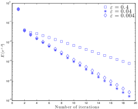
We consider two series of numerical tests for a better understanding of the role of the regularizing parameter $\varepsilon$. In the first series, we fix smalls space and time steps and we vary the regularization parameter $\varepsilon$. In the second series we decrease all the parameters $(\varepsilon,\rho,h)$, respecting the balancing rules in Theorem 3.4.

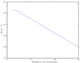
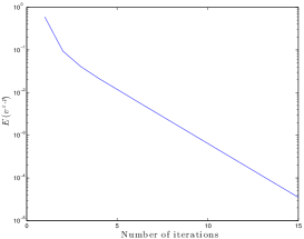
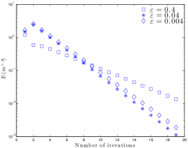
Fig. 1 shows the behavior of the errors (4.2) in logarithmic scale on the $y$-axis versus the number of fixed–point iterations on the $x$-axis. We fixed $\rho=0.0075$, $h=0.015$ and computed 20 fixed-point iterations for each one of the following values of $\varepsilon$: $\varepsilon=0.4$, $\varepsilon=0.04$ and $\varepsilon=0.004$. We observe a slower convergence when $\varepsilon=0.4$ and we get a better and very similar result when $\varepsilon=0.04,0.004$.

Figure 1: Errors: $E(m^{\varepsilon,p})$, $E(v^{\varepsilon,p})$ varying only $\varepsilon$ and keeping the other parameters fixed.

Table 1: Parameters and errors

$\rho$	$h$	$\varepsilon$	$E(v^{\varepsilon,20})$	$E(m^{\varepsilon,20})$
$1.50\cdot 10^{-2}$	$3.00\cdot 10^{-2}$	$6.00\cdot 10^{-2}$	$4.57\cdot 10^{-6}$	$2.08\cdot 10^{-4}$
$7.50\cdot 10^{-3}$	$1.50\cdot 10^{-2}$	$4.00\cdot 10^{-2}$	$1.05\cdot 10^{-5}$	$7.20\cdot 10^{-4}$
$3.75\cdot 10^{-3}$	$7.50\cdot 10^{-3}$	$2.50\cdot 10^{-2}$	$1.04\cdot 10^{-5}$	$9.96\cdot 10^{-4}$
$1.87\cdot 10^{-3}$	$3.75\cdot 10^{-3}$	$1.60\cdot 10^{-2}$	$9.74\cdot 10^{-4}$	$3.56\cdot 10^{-3}$

Figure 2: Errors: $E(m^{\varepsilon,p})$ varying all the parameters $(\varepsilon,\rho,h)$ according to Table 1 (left), $E(m^{\varepsilon,p})$ varying $(\rho,h)$ according to Table 1 and varying the regularizing parameter $\varepsilon$ with smaller values (right).

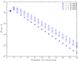
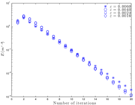
In the second series of numerical tests, we vary all the parameters as shown in Table 1 and for each set of parameters we computed $20$ fixed-point iterations. The parameters have been chosen according to the balance requirements of Theorem 3.4. We observe an increasing trend in the errors with respect to decreasing values of $\varepsilon$. This is due to the fact that we fixed the number of iterations and that smaller are the discretization parameters greater are the number of iterations to reach the fixed error threshold $\tau$.

In Fig.2 (left), we plot the errors for the mass distributions with all the parameters $(\rho,h,\varepsilon)$ varying as in Table 1. We can see that the errors of the fixed point algorithm decreases with the number of fixed point iterations $p$.

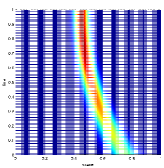
Let us remark that the theoretical balance of parameters in Theorem 3.4 requires to choose the regularizing parameter $\varepsilon$ quite large compared to the space step $\rho$. However, even disregarding this request and choosing to regularize less, i.e. taking $\varepsilon$ smaller, we still get the numerical convergence. This is shown in Fig.2 (right), where we plot the errors for the mass distributions with the parameters $(\rho,h)$ varying as in the first two columns of Table 1 and setting $\varepsilon$ on each row from the top to the bottom equal to $\varepsilon=6.00\cdot 10^{-3}$, $4.00\cdot 10^{-3}$, $2.50\cdot 10^{-3}$ and $1.60\cdot 10^{-3}$, respectively.

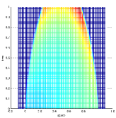
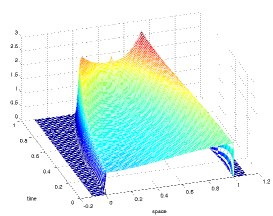
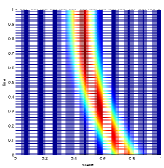
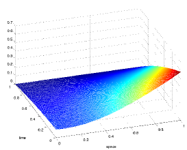
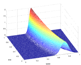
In all the tests, we observe the same shape for the mass and value function evolution. In Fig. 3 we plot the mass evolution in the time–space domain $\Omega\times[0,T]$ for the case $\rho=3.75\cdot 10^{-3}$, $h=7.5\cdot 10^{-3}$ and $\varepsilon=0.025$. We observe that from the initial configuration, the mass distribution tends to avoid the boundary of $\Omega$ and at the same time it does not accumulate completely at the center.

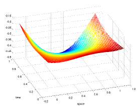
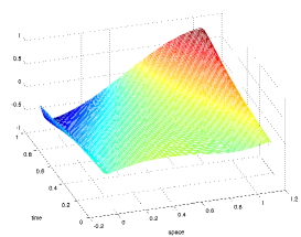
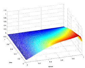
In Fig. 4 the discrete value function $v^{\varepsilon}_{i,k}$ and its gradient $Dv^{\varepsilon}_{i,k}$ are plotted in the domain $\Omega\times[0,T]$.

Figure 3: Mass evolution $m_{i,k}^{\varepsilon}$

Figure 4: Value function $v^{\varepsilon}_{i,k}$ (left) and Gradient $Dv^{\varepsilon}_{i,k}$(right).

4.2 Test 2

We model now a game where the agents want to live at $x=0.2$ but again they are adverse to the presence of other agents. We take as numerical space domain $\Omega=[0,1]$ and final time $T=1$. The running cost function is modeled as

$$\frac{1}{2}\alpha^{2}+F(x,m)=\frac{1}{2}\alpha^{2}+(x-0.2)^{2}+V(x,m),$$

where $V(x,m)$ is defined in (4.3) with $\sigma=0.25$. We do not consider a final cost, i.e. we take $G\equiv 0$. We choose as initial mass distribution:

$$m_{0}(x)=\frac{\nu(x)}{\int_{\Omega}\nu(x)dx},\;{\rm with}\;\nu(x)=e^{-(x-0.75)^{2}/(0.1)^{2}}.$$

We choose as space discretization step $\rho=3.3\cdot 10^{-3}$, as time step $h=0.005$ and as regularization parameter $\varepsilon=0.025$. We perform fixed-point iterations until the error threshold $\tau=10^{-3}$ is reached. This is achieved after $15$ iterations.

Figure 5: Mass distribution $m^{\varepsilon}_{i,k}$.

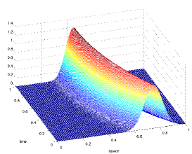
Fig. 5 shows the mass evolution. As it is expected, during the evolution the mass distribution tends to concentrate at the “low energy” configuration $x=0.2$ and at the same time the second term in $F$ penalize high mass concentrations. The discrete value function and its gradient are plotted in Fig. 6 and in Fig. 7 we display the errors $E(m^{\varepsilon,p})$ and $E(v^{\varepsilon,p})$ of the fixed–point iterations.

Figure 6: Value function $v^{\varepsilon}_{i,k}$ (left) and Gradient $Dv^{\varepsilon}_{i,k}$(right).

Figure 7: Errors: $E(m^{\varepsilon,p})$ (left),  $E(v^{\varepsilon,p})$ (right), $\;p=0....,15$.

Let us finally compare this test to the case when there is no game, i.e. the running cost does not depend on $m$:

$$F(x,m)=(x-0.2)^{2}.$$

In this case, the system is not coupled and after one iteration we obtain the solution.
In Fig. 8, the mass evolution is shown. It is seen that, during the evolution, the measure is allowed to concentrate, due to the absence of a high mass penalization term in $F$. This shows qualitative differences with the results plotted in Fig. 5, where conflict between the agents was present.

Figure 8: Mass distribution $m^{\varepsilon}_{i,k}$ (case “no game” with $F=(x-0.2)^{2}$ ).

References

- [1] Y. Achdou, F. Camilli, and I. Capuzzo-Dolcetta. Mean field games: numerical methods for the planning problem. SIAM J. Control Optim., 50(1):77–109, 2012.
- [2] Y. Achdou, F. Camilli, and I. Capuzzo Dolcetta. Mean field games: convergence of a finite difference method. Preprint, 2012.
- [3] Y. Achdou, F. Camilli, and L.Corrias. On numerical approximations of the Hamillton-Jacobi-transport system arysing in high frequency. Preprint, 2011.
- [4] Y. Achdou and I. Capuzzo-Dolcetta. Mean field games: numerical methods. SIAM J. Numer. Anal., 48(3):1136–1162, 2010.
- [5] L. Ambrosio, N. Gigli, and G. Savaré. Gradient flows in metric spaces and in the space of probability measures. Lectures in Mathematics ETH Zürich. Birkhäuser Verlag, Basel, second edition, 2008.
- [6] J.-P. Aubin and H. Frankowska. Set-valued analysis, volume 2 of Systems & Control: Foundations & Applications. Birkhäuser Boston Inc., Boston, MA, 1990.
- [7] R. Aumann. Markets with a continuum of traders. Econometrica, 32(1/2), 1964.
- [8] M. Bardi and I. Capuzzo-Dolcetta. Optimal control and viscosity solutions of Hamilton-Jacobi-Bellman equations. Systems & Control: Foundations & Applications. Birkhäuser Boston Inc., Boston, MA, 1997. With appendices by Maurizio Falcone and Pierpaolo Soravia.
- [9] G. Barles and P.E. Souganidis. Convergence of approximation schemes for fully nonlinear second order equations. Asymptotic Anal., 4(3):271–283, 1991.
- [10] F. Camilli and F. J. Silva. A semi-discrete in time approximation for a first order-finite mean field game problem. Network and Heterogeneous Media, 7-2:263–277, 2012.
- [11] P. Cannarsa and C. Sinestrari. Semiconcave functions, Hamilton-Jacobi equations, and optimal control. Progress in Nonlinear Differential Equations and their Applications, 58. Birkhäuser Boston Inc., Boston, MA, 2004.
- [12] P. Cardaliaguet. Notes on mean field games: from P.-L. Lions’ lectures at Collège de France. Lecture Notes given at Tor Vergata, 2010.
- [13] E. Carlini, M. Falcone, and R. Ferretti. Convergence of a large time-step scheme for mean curvature motion. Interfaces Free Bound., 12(4):409–441, 2010.
- [14] P. G. Ciarlet and J.-L. Lions, editors. Handbook of numerical analysis. Vol. II. Handbook of Numerical Analysis, II. North-Holland, Amsterdam, 1991. Finite element methods. Part 1.
- [15] M. Falcone and R. Ferretti. Semi-Lagrangian Approximation Schemes for Linear and Hamilton-Jacobi Equations. MOS-SIAM Series on Optimization, to appear.
- [16] L. Gosse and F. James. Convergence results for an inhomogeneous system arising in various high frequency approximations. Numer. Math., 90(4):721–753, 2002.
- [17] O. Guéant. Mean field games equations with quadratic hamiltonian: a specific approach. Mathematical Models and Methods in Applied Sciences, 22, 2012.
- [18] O. Guéant, J.-M-Lasry, and P.-L. Lions. Mean field games and applications. In Paris-Princeton Lectures on Mathematical Finance 2010, volume 2003 of Lecture Notes in Math., pages 205–266. Springer, Berlin, 2011.
- [19] A. Lachapelle and M.-T. Wolfram. On a mean field game approach modeling congestion and aversion in pedestrian crowds. Transportation Research Part B: Methodological, 45:1572–1589, 2011.
- [20] J.-M. Lasry and P.-L. Lions. Jeux à champ moyen. I. Le cas stationnaire. C. R. Math. Acad. Sci. Paris, 343(9):619–625, 2006.
- [21] J.-M. Lasry and P.-L. Lions. Jeux à champ moyen. II. Horizon fini et contrôle optimal. C. R. Math. Acad. Sci. Paris, 343(10):679–684, 2006.
- [22] J.-M. Lasry and P.-L. Lions. Mean field games. Jpn. J. Math., 2:229–260, 2007.
- [23] C.-T. Lin and E. Tadmor. -stability and error estimates for approximate Hamilton-Jacobi solutions. Numer. Math., 87(4):701–735, 2001.
- [24] P.-L. Lions. Cours au Collège de France. www.college-de-france.fr, 2007-2008.
- [25] S. Osher and R. Fedkiw. Level set methods and dynamic implicit surfaces, volume 153 of Applied Mathematical Sciences. Springer-Verlag, New York, 2003.
- [26] B. Piccoli and A. Tosin. Time-evolving measures and macroscopic modeling of pedestrian flow. Arch. Ration. Mech. Anal., 199(3):707–738, 2011.
- [27] F. Poupaud. and M. Rascle. Measure solutions to the linear multi-dimensional transport equation with non-smooth coefficients. Comm. Partial Differential Equations, 22(1-2):337–358, 1997.
- [28] A. Quarteroni, R. Sacco, and F. Saleri. Numerical Mathematics (Second Ed.). Springer, Berlin, 2007.
- [29] J. A. Sethian. Level set methods and fast marching methods, volume 3 of Cambridge Monographs on Applied and Computational Mathematics. Cambridge University Press, Cambridge, second edition, 1999. Evolving interfaces in computational geometry, fluid mechanics, computer vision, and materials science.
- [30] A. Tosin and P. Frasca. Existence and approximation of probability measure solutions to models of collective behaviors. Netw. Heterog. Media, 6(3):561–596, 2011.