Emergent Nesting of the Fermi Surface from Local-Moment Description of Iron-Pnictide High-$T_{c}$ Superconductors

Abstract

We uncover the low-energy spectrum of a $t$-$J$ model for electrons on a square lattice of spin-$1$ iron atoms with $3d_{xz}$ and $3d_{yz}$ orbital character by applying Schwinger-boson-slave-fermion mean-field theory and by exact diagonalization of one hole roaming over a $4\times 4\times 2$ lattice. Hopping matrix elements are set to produce hole bands centered at zero two-dimensional (2D) momentum in the free-electron limit. Holes can propagate coherently in the $t$-$J$ model below a threshold Hund coupling when long-range antiferromagnetic order across the $d+=3d_{(x+iy)z}$ and $d-=3d_{(x-iy)z}$ orbitals is established by magnetic frustration that is off-diagonal in the orbital indices. This leads to two hole-pocket Fermi surfaces centered at zero 2D momentum. Proximity to a commensurate spin-density wave (cSDW) that exists above the threshold Hund coupling results in emergent Fermi surface pockets about cSDW momenta at a quantum critical point (QCP). This motivates the introduction of a new Gutzwiller wavefunction for a cSDW metal state. Study of the spin-fluctuation spectrum at cSDW momenta indicates that the dispersion of the nested band of one-particle states that emerges is electron-type. Increasing Hund coupling past the QCP can push the hole-pocket Fermi surfaces centered at zero 2D momentum below the Fermi energy level, in agreement with recent determinations of the electronic structure of mono-layer iron-selenide superconductors.

1 Introduction

The surprising discovery of high-temperature superconductivity in iron-pnictide compounds is one of the more recent unsolved puzzles in condensed matter physics[1]. Determinations of the electronic structure in these superconductors by angle-resolved photo-emission spectroscopy (ARPES) find hole bands that form Fermi surface pockets at zero two-dimensional (2D) momentum and electron bands that form Fermi surface pockets at 2D momenta $(\pi/a){\hat{\bi x}}$ and $(\pi/a){\hat{\bi y}}$ [2][3][4][5]. Here $a$ denotes the lattice constant of the square lattice of iron atoms that stacks up to form iron-pnictide materials. Calculations of the electronic band structure that include all five iron $3d$ orbitals, but that assume only weak inter-electron repulsion, are consistent with the ARPES results[6][7][8]. By contrast, the simplest tight-binding model for the electronic structure of iron-pnictide materials that include only the $3d_{xz}$ and $3d_{yz}$ orbitals can also produce such nested Fermi surface pockets[9], but it predicts a Fermi surface pocket at 2D momentum $(\pi/a)({\hat{\bi x}}+{\hat{\bi y}})$ with a spectral weight that is much too strong[8]. Iron-pnictide superconductors also have parent compounds that exhibit weak commensurate spin-density-wave (cSDW) order at low temperature. The ordered cSDW moment measured by elastic neutron diffraction can reach values as low as $0.3$ Bohr magnetons ($\mu_{B}$) [10]. By comparison, band structure calculations predict an ordered magnetic moment of $2\,\mu_{B}$ that is much larger. Frustrated Heisenberg models that assume local magnetic moments at each iron atom can successfully account for the weak cSDW that exists in parent compounds[11][12][13][14], on the other hand. They can also give a good account of the low-energy spin excitations near cSDW momenta that have been uncovered in iron-pnictide systems by inelastic neutron scattering[15][16][17][18][19][20]. Such Heisenberg models have an insulating groundstate, however, that is a result of strong inter-electron repulsion. This fact conflicts with the metallic nature of iron-pnictide superconductors and their parent compounds.

We identify a way to resolve this dilemma from the limit of strong inter-electron repulsion by injecting a low concentration of mobile hole charges into a local-moment cSDW[12]. Spin-1/2 electrons are localized on $d+=3d_{(x+iy)z}$ and $d-=3d_{(x-iy)z}$ orbitals of each iron site, and they can hop to unoccupied orbitals in neighboring iron atoms. The $d{\pm}$ orbital basis maximizes the Hund’s Rule coupling, which therefore maximizes the tendency to form local magnetic moments per iron atom. Hopping matrix elements are chosen to produce 2D hole bands centered at zero momentum. As Hund’s Rule coupling weakens, both Schwinger-boson-slave-fermion mean-field theory and exact computer calculations for one hole that roams over a $4\times 4$ lattice find evidence for a quantum phase transition into a hidden half-metal state that shows long-range antiferromagnetic order across the $d+$ and $d-$ orbitals[21]. Coherent intra-orbital hole motion persists because of the hidden magnetic order. This yields two Fermi surface hole pockets centered at zero 2D momentum. Nested Fermi surface pockets emerge at cSDW momenta as Hund coupling increases past the quantum critical point. (See Fig. 8.) In particular, the exact calculations find nested one-particle states at wavenumbers $(\pi/a){\hat{\bi x}}$ and $(\pi/a){\hat{\bi y}}$ that have predominantly $3d_{yz}$ and $3d_{xz}$ orbital character, respectively. (See Fig. 5.) This inspires us to introduce a new Gutzwiller wavefunction[22] in section 5 that exhibits a low carrier density and cSDW nesting. Further, study of the spectrum for cSDW spin fluctuations in the present local-moment description argues strongly for electron-type dispersion of the emergent Fermi surface pockets.

The local-moment description that we use to describe low-energy electronic physics in iron superconductors makes two additional predictions. First, zero-energy hidden spin-wave excitations across the $d+$ and $d-$ orbitals are present in the hidden half metal at the long wavelength limit. We show that these persist at low energy in the cSDW metal state because of nesting between the two $d_{xz}$-$d_{yz}$ hole-pocket Fermi surfaces that are centered at zero 2D momentum, albeit with much reduced spectral weight. The new Gutzwiller wavefunction introduced in section 5 is used to demonstrate this. We point out that such low-energy hidden spin fluctuations are predicted by density functional theory (DFT) calculations that exhibit similar hole-pocket Fermi surfaces[6][7][8]. Second, the fact that $d_{xz}$-$d_{yz}$ hole bands lie below the Fermi surface in new interfacial iron-selenide superconductors[23][24][25][26] is explained naturally in our model by moving off the quantum-critical point that separates the hidden half metal from a cSDW metal. Single-layer iron selenides have attained record critical temperatures within the class of iron superconductors. DFT calculations, by comparison, typically yield that the $d_{xz}$-$d_{yz}$ hole bands cross the Fermi surface in interfacial iron selenides[27].

2 Two-Orbital t-J Model

We shall now introduce a $t$-$J$ model that describes the low-energy excitations of electrons with $3d_{xz}$ and $3d_{yz}$ orbital character in iron-pnictide high-temperature superconductors[21]. Spin-1/2 moments exist over the $3d_{(x+iy)z}$ and $3d_{(x-iy)z}$ orbitals at each iron atom. These are the least localized orbitals within the 2D subspace spanned by the degenerate $3d_{xz}$ and $3d_{yz}$ orbitals, and they therefore result in the largest possible Hund’s Rule coupling constant, $-J_{0}$. This fact is demonstrated explicitly in Appendix A for the case of hydrogenic $3d$ orbitals with the bare Coulomb interaction. In contrast, the commonly used $3d_{xz}$ and $3d_{yz}$ orbitals from Chemistry are the most localized ones within the same 2D subspace[28][29][30], and they result in the smallest possible Hund’s Rule coupling. The isotropic nature of the $3d_{(x\pm iy)z}$ orbitals also implies isotropic Heisenberg exchange coupling constants $J_{1}$ and $J_{2}$ across nearest-neighbor and next-nearest-neighbor links of the square lattice of iron atoms within each iron-pnictide layer. The two-orbital $t$-$J$ model over a square-lattice of iron atoms in an isolated layer then reads

$$H= -\sum_{\langle i,j\rangle}\sum_{\alpha,\beta}\sum_{s}(t_{1}^{\alpha,\beta}c_{i,\alpha,s}^{\dagger}c_{j,\beta,s}+{\rm h.c.})-\sum_{\langle\langle i,j\rangle\rangle}\sum_{\alpha,\beta}\sum_{s}(t_{2}^{\alpha,\beta}c_{i,\alpha,s}^{\dagger}c_{j,\beta,s}+{\rm h.c.})$$

$$+{1\over 2}J_{0}\sum_{i}\biggl{[}\sum_{\alpha}{\bi S}_{i,\alpha}\biggr{]}^{2}+\sum_{\langle i,j\rangle}\sum_{\alpha,\beta}J_{1}^{\alpha,\beta}{\bi S}_{i,\alpha}\cdot{\bi S}_{j,\beta}+\sum_{\langle\langle i,j\rangle\rangle}\sum_{\alpha,\beta}J_{2}^{\alpha,\beta}{\bi S}_{i,\alpha}\cdot{\bi S}_{j,\beta}$$

$$+{\rm lim}_{U_{0}\rightarrow\infty}\sum_{i}\sum_{\alpha}U_{0}n_{i,\alpha,\uparrow}n_{i,\alpha,\downarrow}+\sum_{i}U_{0}^{\prime}n_{i,d+}n_{i,d-}.$$

Above, ${\bi S}_{i,\alpha}$ is the spin operator that acts on the spin $s_{0}=1/2$ state localized on orbital $\alpha$ at site $i$, while $c_{i,\alpha,s}^{\dagger}$ is the corresponding electron creation operator. The orbitals $\alpha$ are either $d+=3d_{(x+iy)z}$ or $d-=3d_{(x-iy)z}$ , while the sites $i$ run over the square lattice of iron atoms. The constraint against double-occupancy at a site-orbital is enforced by the divergent Hubbard term, where $n_{i,\alpha,s}=c_{i,\alpha,s}^{\dagger}c_{i,\alpha,s}$ is the occupation operator. Also, the last term above gives the energy cost for a pair of holes at an iron site, $U_{0}^{\prime}>0$, where $n_{i,\alpha}=n_{i,\alpha,\uparrow}+n_{i,\alpha,\downarrow}$. The isotropy and the degeneracy of the $d+$ and $d-$ orbital states yields two independent and isotropic Heisenberg exchange coupling constants for nearest-neighbor and for next-nearest-neighbor links, $\langle i,j\rangle$ and $\langle\langle i,j\rangle\rangle$, respectively, $n=1$ and $2$:

$$J_{n}^{d+,d+}=J_{n}^{\parallel}=J_{n}^{d-,d-}\quad{\rm and}\quad J_{n}^{d+,d-}=J_{n}^{\perp}=J_{n}^{d-,d+}.$$ (2)

Correlated hopping of an electron in orbital $\beta$ to a neighboring unoccupied orbital $\alpha$ is controlled by the hopping matrix elements $t_{1}^{\alpha,\beta}$ and $t_{2}^{\alpha,\beta}$. Let us take real hopping matrix elements in the $(3d_{xz},3d_{yz})$ orbital basis[9]. The hopping matrix elements in the present $d\pm$ basis are then given by

$$t_{n}^{d\pm,d\pm}={1\over 2}[t_{n}^{x,x}+t_{n}^{y,y}]\pm{i\over 2}[t_{n}^{x,y}-t_{n}^{y,x}],$$ (3a)

$$t_{n}^{d\pm,d\mp}={1\over 2}[t_{n}^{x,x}-t_{n}^{y,y}]\mp{i\over 2}[t_{n}^{x,y}+t_{n}^{y,x}].$$ (3b)

The symmetry relation $t_{1(2)}^{x,y}=t_{1(2)}^{y,x}$ in the $(3d_{xz},3d_{yz})$ orbital basis then yields diagonal hopping matrix elements that are real and isotropic in the $(d+$, $d-)$ basis:

$$\qquad t_{1}^{d\pm,d\pm}(\hat{\bi x}) =t_{1}^{d\pm,d\pm}(\hat{\bi y}) \quad{\rm and}\quad{\rm Im}\,t_{1}^{d\pm,d\pm}=0,$$ (3da)

$$t_{2}^{d\pm,d\pm}({\hat{\bi}x}+{\hat{\bi}y}) =t_{2}^{d\pm,d\pm}({\hat{\bi y}}-\hat{\bi x}) \quad{\rm and}\quad{\rm Im}\,t_{2}^{d\pm,d\pm}=0.$$ (3db)

The off-diagonal hopping matrix elements $t_{n}^{d\pm,d\mp}$ have $d$-wave symmetry, on the other hand. Also, the identities $t_{1}^{x,y}=0=t_{1}^{y,x}$ yields real off-diagonal hopping matrix elements across nearest neighbors, while the symmetry relation $t_{2}^{x,x}=t_{2}^{y,y}$ yields pure-imaginary off-diagonal hopping matrix elements across next-nearest neighbors:

$$\qquad t_{1}^{d\pm,d\mp}(\hat{\bi x}) =-t_{1}^{d\pm,d\mp}(\hat{\bi y}) \quad{\rm and}\quad{\rm Im}\,t_{1}^{d\pm,d\mp}=0,$$ (3dea)

$$t_{2}^{d\pm,d\mp}(\hat{\bi x}+\hat{\bi y}) =-t_{2}^{d\pm,d\mp}(\hat{\bi y}-\hat{\bi x}) \quad{\rm and}\quad{\rm Re}\,t_{2}^{d\pm,d\mp}=0.$$ (3deb)

Henceforth, we shall change the notation for the hopping matrix elements to $t_{1(2)}^{\parallel}=t_{1(2)}^{d\pm,d\pm}$, to $t_{1}^{\perp}=t_{1}^{d\pm,d\mp}$, and to $-t_{2}^{d-,d+}=t_{2}^{\perp}=t_{2}^{d+,d-}$.

Last, it is useful to point out that because $t_{1}^{\perp}$ is real, a global swap of the orbitals, $d\pm\rightarrow d\mp$, is an exact symmetry of the two-orbital $t$-$J$ model (LABEL:tJ) in the absence of next-nearest neighbor inter-orbital hopping: $t_{2}^{\perp}=0$. Let $P_{d\bar{d}}$ denote the global swap operation of the $d+$ and $d-$ orbitals. Eigenstates of the $t$-$J$ model Hamiltonian (LABEL:tJ) are then even ($+$) or odd ($-$) under it, with respective forms $|\Psi\rangle\pm P_{d\bar{d}}|\Psi\rangle$. Further, in the limit $J_{0}\rightarrow-\infty$ where Hund’s Rule is obeyed, a spin triplet state exists at iron atoms that do not have any holes. Such spin-$1$ local moments are clearly even under $P_{d\bar{d}}$. This implies that a one-hole state that is even under $P_{d\bar{d}}$ is in a local $3d_{xz}$ orbital when Hund’s Rule is obeyed, and that a one-hole state that is odd under $P_{d\bar{d}}$ is in a local $3d_{yz}$ orbital. At the opposite extreme $J_{0}\rightarrow+\infty$ where Hund’s Rule is maximally violated, a spin singlet state exists at iron atoms without any holes. Such spin-$0$ iron sites are clearly odd under $P_{d\bar{d}}$. In the case of an even number of iron sites, this implies that a one-hole state that is even under $P_{d\bar{d}}$ instead is in a local $3d_{yz}$ orbital, and that a one-hole state that is odd under $P_{d\bar{d}}$ instead is in a local $3d_{xz}$ orbital! One-hole states that are even or odd under $P_{d\bar{d}}$ must then have a mixture of $3d_{xz}$ and $3d_{yz}$ orbital character at finite Hund’s Rule coupling by continuity.

And because $t_{2}^{\perp}$ is pure imaginary, the global orbital swap operation is an exact symmetry in the absence of nearest-neighbor inter-orbital hopping, $t_{1}^{\perp}=0$, after making the global gauge transformation of the orbitals $|d\pm\rangle\rightarrow i^{\pm 1/2}|d\pm\rangle$. Eigenstates of the $t$-$J$ model Hamiltonian (LABEL:tJ) are then even ($+$) or odd ($-$) under the combined operation $P_{d\bar{d}}^{\prime}$, where they have the form $|\Psi\rangle\pm P_{d\bar{d}}^{\prime}|\Psi\rangle$. Notice that the global gauge transformation rotates the orbital axes by 45 degrees. Repeating the previous arguments yields that a one-hole state that is even under $P_{d\bar{d}}^{\prime}$ is in a local $3d_{x^{\prime}z}$ orbital when Hund’s Rule is obeyed, and that a one-hole state that is odd under $P_{d\bar{d}}^{\prime}$ is in a local $3d_{y^{\prime}z}$ orbital in such case. Here $(x^{\prime},y^{\prime})$ denote the planar orbital coordinates along the next-nearest-neighbor links.

It is possible that iron-pnictide materials show low-energy electronic excitations with orbital character other than $3d_{xz}$ and $3d_{yz}$. DFT calculations predict that certain Fermi surfaces have $3d_{xy}$ orbital character, for example[8]. We work within the approximation that the Hamiltonian that describes the remaining set of orbitals commutes with the two-orbital $t$-$J$ model (LABEL:tJ). In more physical terms, we therefore assume that all Fermi surfaces with $3d_{xz}$ or $3d_{yz}$ character have no other orbital content. A recent report of electronic structure in optimally doped Ba(Fe_1-xCo_x)₂As₂ from ARPES is consistent with this restriction [5].

3 Hidden Half Metal State

In general, the Heisenberg exchange constants have a direct ferromagnetic contribution from the exchange Coulomb integral and an indirect antiferromagnetic contribution from the super-exchange mechanism through the pnictide atom[11][31]:

$$J_{1(2)}^{\alpha,\beta}=J_{1(2)}^{\alpha,\beta}({\rm drct})+J_{1(2)}^{\alpha,\beta}({\rm sprx}).$$ (3def)

We shall assume that the super-exchange contribution is independent of the orbital indices: $J_{1(2)}^{\alpha,\beta}({\rm sprx})=J_{1(2)}^{({\rm sprx})}$. This is the case if the pnictide orbital in question is the $p_{x}$, $p_{y}$, or $p_{z}$ one, for example. Recent density-functional theory calculations for the electronic structure of iron-pnictide materials find that direct exchange and super exchange can cancel out across nearest neighbors[32][33]. More generally, we shall assume that $J_{1(2)}^{d\pm,d\mp}({\rm drct})$ is much smaller in magnitude than $J_{1(2)}^{d\pm,d\pm}({\rm drct})$. This assumption is borne out in the limit of large overlap between neighboring iron $3d$ orbitals, where $-J_{1(2)}^{d\pm,d\mp}({\rm drct})$ is $10$ times smaller than $-J_{1(2)}^{d\pm,d\pm}({\rm drct})$. [See Appendix A, Eq. (3desacajbnca).] We are then left with a net antiferromagnetic Heisenberg exchange (3def) across nearest neighbors between different orbitals due to super-exchange, $J_{1}^{\perp}>0$, and with a net nearest-neighbor Heisenberg exchange (3def) across the same orbital that is weaker, and possibly even ferromagnetic, $J_{1}^{\parallel}<J_{1}^{\perp}$. Last, DFT calculations find that $J_{2}^{\alpha,\beta}({\rm drct})$ is negligible[32]. This leaves antiferromagnetic Heisenberg exchange across next-nearest neighbors due to super-exchange, which we have assumed to be invariant with respect to a rotation of the orbital basis: $J_{2}^{\parallel}=J_{2}^{\perp}>0$.

In the absence of mobile holes, the off-diagonal magnetic frustration described by the above list of Heisenberg exchange constants results in a commensurate spin-density wave (cSDW) along one of the principal axes of the square lattice of iron atoms at strong Hund’s Rule coupling, $-J_{0}$, and for $J_{2}>J_{1}/2$. Here $J_{1(2)}=(J_{1(2)}^{\parallel}+J_{1(2)}^{\perp})/2$. An antiferromagnetic state with ferromagnetic order over the $d+$ and the $d-$ orbitals of opposite sign appears at Hund’s Rule coupling below a critical value of $-J_{0c}=2(J_{1}^{\perp}-J_{1}^{\parallel})-4J_{2}^{\parallel}$ in the large-$s_{0}$ limit[14]. We call this state a hidden ferromagnet because it displays no net ordered magnetic moment. The critical Hund coupling, $-J_{0c}$, marks a quantum-critical phase transition between the cSDW at strong Hund’s Rule coupling and the hidden ferromagnet at weak Hund’s Rule coupling. (Cf. Fig. 1.) Observe now that injecting mobile holes while inter-orbital hopping is suppressed preserves the $\nwarrow_{d+}\searrow_{d-}$ spin order of the hidden ferromagnetic state in the classical limit[14]. This is a semi-classical picture of a hidden half-metal state with coherent propagation of holes within each $d\pm$ orbital that follows the dispersion relation

$$\varepsilon_{e}({\bi k})=-2t_{1}^{\parallel}(\cos\,k_{x}a+\cos\,k_{y}a)-2t_{2}^{\parallel}(\cos\,k_{+}a+\cos\,k_{-}a),$$ (3deg)

where $k_{\pm}=k_{x}\pm k_{y}$. It implies two degenerate hole Fermi surface pockets centered at zero momentum when $t_{1}^{\parallel}<0$ and $t_{1}^{\parallel}+2t_{2}^{\parallel}<0$, in qualitative agreement with ARPES on iron-pnictide superconductors. Below, we shall demonstrate that the hidden half-metal state is robust with respect to the addition of inter-orbital hopping. We will also find emergent cSDW nesting at the quantum-critical point that separates the hidden half-metal state from the cSDW state. It results in copies of the hole Fermi-surface pockets centered at cSDW wavenumbers $(\pi/a){\hat{\bi x}}$ and $(\pi/a){\hat{\bi y}}$ [21]. We shall argue in section 5 that the dispersion of the latter is electron type.

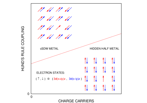
Figure 1: Shown is the phase diagram obtained from the Schwinger-boson-slave-fermion mean-field theory of the two-orbital $t$-$J$ model, Eq. (LABEL:tJ). The red line marks a quantum-critical point that separates a charge-carrier poor cSDW metal from a charge-carrier rich hidden half metal at fixed Hund’s Rule coupling.

3.1 Schwinger-Boson-Slave-Fermion Mean-field Theory

Unlike the doped Néel state in the one-orbital nearest-neighbor $t$-$J$ model for copper-oxygen planes in high-$T_{c}$ superconductors[34][35], hole propagation in the hidden half metal does not produce strings of overturned spins that disrupt the antiferromagnetic $\nwarrow_{d+}\searrow_{d-}$ order when inter-orbital hopping is absent. This suggests that the mean-field approximation for the Schwinger-boson-slave-fermion formulation of the two-orbital $t$-$J$ model (LABEL:tJ) can be applied to this state at weak inter-orbital hopping. Within that approximation, we show below that the hidden half-metal state survives the introduction of inter-orbital hopping by dynamically suppressing it.

The constraint against double occupancy in the $t$-$J$ model (LABEL:tJ) can be enforced by replacing the electron annihilation operator with a correlated electron annihilation operator $\tilde{c}_{i,\alpha,s}=b_{i,\alpha,s}f_{i,\alpha}^{\dagger}$ along with a new constraint per site $i$, per orbital $\alpha$,

$$2s_{0}=b_{i,\alpha,\uparrow}^{\dagger}b_{i,\alpha,\uparrow}+b_{i,\alpha,\downarrow}^{\dagger}b_{i,\alpha,\downarrow}+f_{i,\alpha}^{\dagger}f_{i,\alpha},$$ (3deh)

where $s_{0}=1/2$ is the electron spin [36][37]. Here, $b_{i,\alpha,\uparrow}$ and $b_{i,\alpha,\downarrow}$ are the annihilation operators for a pair of Schwinger bosons, while $f_{i,\alpha}$ is the annihilation operator for a spinless slave fermion. The spin operator is then expressed in the usual way: ${\bi S}_{i,\alpha}={1\over 2}\hbar\sum_{s,s{\prime}}f_{i,\alpha}b_{i,\alpha,s}^{\dagger}{\boldsymbol{\sigma}}_{s,s^{\prime}}b_{i,\alpha,s^{\prime}}f_{i,\alpha}^{\dagger}$. Henceforth, we shall average the dynamics of the slave fermions over the bulk by writing ${\bi S}_{i,\alpha}\cong(1-x){1\over 2}\hbar\sum_{s,s{\prime}}b_{i,\alpha,s}^{\dagger}{\boldsymbol{\sigma}}_{s,s^{\prime}}b_{i,\alpha,s^{\prime}}$ instead. Here, $x$ denotes the concentration of holes per orbital. We shall also henceforth neglect hole-hole repulsion at iron sites, $U_{0}^{\prime}$, which should be a valid approximation at low $x$. Following Arovas and Auerbach[38][39], we introduce symmetric versus antisymmetric mean fields with respect to spin flip for the ferromagnetic versus the antiferromagnetic links of the hidden ferromagnetic state (Fig. 1):

$$\langle b_{i,d\pm,\downarrow}^{\dagger}b_{j,d\pm,\downarrow}\rangle=Q_{n}^{\parallel}=\langle b_{i,d\pm,\uparrow}^{\dagger}b_{j,d\pm,\uparrow}\rangle\qquad(n=1,2),$$ (3dei)

$$\pm \langle b_{i,d\pm,\downarrow}b_{j,d\mp,\uparrow}\rangle=Q_{n}^{\perp}=\mp\langle b_{i,d\pm,\uparrow}b_{j,d\mp,\downarrow}\rangle\qquad(n=0,1,2),$$ (3dej)

where $j=i$ for on-site links $n=0$, where $j=i+\hat{\bi x}(\hat{\bi y})$ for nearest-neighbor links $n=1$, and where $j=i\pm\hat{\bi x}+\hat{\bi y}$ for next-nearest-neighbor links $n=2$. Next, we introduce meanfields associated with hopping by slave fermions:

$${1\over 2}\langle f_{i,d+}^{\dagger}f_{j,d+}\rangle= P_{n}^{\parallel}={1\over 2}\langle f_{i,d-}^{\dagger}f_{j,d-}\rangle,$$ (3dek)

$${1\over 2}\langle f_{i,d+}^{\dagger}f_{j,d-}\rangle^{*}= P_{n}^{\perp}={1\over 2}\langle f_{i,d-}^{\dagger}f_{j,d+}\rangle\qquad(n=1,2).$$ (3del)

Last, we introduce meanfields associated with hopping of the Schwinger bosons across different orbitals:

$$\langle b_{i,d+,s}^{\dagger}b_{j,d-,s}\rangle^{*}=R_{n}^{\perp}=\langle b_{i,d-,s}^{\dagger}b_{j,d+,s}\rangle\qquad(n=1,2),$$ (3dem)

where $s=\uparrow,\downarrow$. Notice that all of the mean fields show invariance under orbital swap. Now assume that all of the mean fields are also homogeneous, and assume that the mean fields $P_{1(2)}^{\parallel}$, $Q_{1(2)}^{\parallel}$ and $Q_{1(2)}^{\perp}$ are isotropic. The mean-field approximation for the $t$-$J$ model Hamiltonian (LABEL:tJ) then has the form $H_{MF}=H_{0}[P,Q,R]+H_{b}^{(+)}+H_{b}^{(-)}+H_{f}$, where

$$H_{0}= 2\sum_{i}J_{0}^{\prime}Q_{0}^{\perp}Q_{0}^{\perp*}+$$

$$2\sum_{\langle i,j\rangle}\sum_{\alpha}[-(2t_{1}^{\parallel}Q_{1}^{\parallel}P_{1}^{\parallel}+{\rm c.c.})-J_{1}^{\prime\parallel}Q_{1}^{\parallel}Q_{1}^{\parallel*}]+$$

$$2\sum_{\langle i,j\rangle}\sum_{\alpha}[-(2t_{1}^{\perp}R_{1}^{\perp}P_{1}^{\perp}+{\rm c.c.})+J_{1}^{\prime\perp}Q_{1}^{\perp}Q_{1}^{\perp*}]+$$

$$2\sum_{\langle\langle i,j\rangle\rangle}\sum_{\alpha}[-(2t_{2}^{\parallel}Q_{2}^{\parallel}P_{2}^{\parallel}+{\rm c.c.})-J_{2}^{\prime\parallel}Q_{2}^{\parallel}Q_{2}^{\parallel*}]+$$

$$2\sum_{\langle\langle i,j\rangle\rangle}\sum_{\alpha}[-(2t_{2}^{\perp}R_{2}^{\perp}P_{2}^{\perp}+{\rm c.c.})+J_{2}^{\prime\perp}Q_{2}^{\perp}Q_{2}^{\perp*}]$$

consolidates the bilinear terms among the mean fields, where

$$H_{b}^{(+)}={1\over 2}\sum_{\bi k}\left[{\begin{array}[]{c}b_{d+,\uparrow}\\ b_{d-,\uparrow}\\ {\bar{b}}_{d+,\downarrow}^{\dagger}\\ {\bar{b}}_{d-,\downarrow}^{\dagger}\end{array}}\right]^{\dagger}\left[{\begin{array}[]{cccc}\Omega_{\parallel}&\Omega_{\perp}^{\prime*}&0&+\Omega_{\perp}\\ \Omega_{\perp}^{\prime}&\Omega_{\parallel}&-\Omega_{\perp}&0\\ 0&-\Omega_{\perp}&\Omega_{\parallel}&\Omega_{\perp}^{\prime}\\ +\Omega_{\perp}&0&\Omega_{\perp}^{\prime*}&\Omega_{\parallel}\end{array}}\right]\left[{\begin{array}[]{c}b_{d+,\uparrow}\\ b_{d-,\uparrow}\\ {\bar{b}}_{d+,\downarrow}^{\dagger}\\ {\bar{b}}_{d-,\downarrow}^{\dagger}\end{array}}\right]$$

and

$$H_{b}^{(-)}={1\over 2}\sum_{\bi k}\left[{\begin{array}[]{c}b_{d+,\downarrow}\\ b_{d-,\downarrow}\\ {\bar{b}}_{d+,\uparrow}^{\dagger}\\ {\bar{b}}_{d-,\uparrow}^{\dagger}\end{array}}\right]^{\dagger}\left[{\begin{array}[]{cccc}\Omega_{\parallel}&\Omega_{\perp}^{\prime*}&0&-\Omega_{\perp}\\ \Omega_{\perp}^{\prime}&\Omega_{\parallel}&+\Omega_{\perp}&0\\ 0&+\Omega_{\perp}&\Omega_{\parallel}&\Omega_{\perp}^{\prime}\\ -\Omega_{\perp}&0&\Omega_{\perp}^{\prime*}&\Omega_{\parallel}\end{array}}\right]\left[{\begin{array}[]{c}b_{d+,\downarrow}\\ b_{d-,\downarrow}\\ {\bar{b}}_{d+,\uparrow}^{\dagger}\\ {\bar{b}}_{d-,\uparrow}^{\dagger}\end{array}}\right]$$

are the pair of Hamiltonians for free Schwinger bosons, with matrix elements

$$\Omega_{\parallel}({\bi k})= \lambda+4\sum_{n=1,2}(J_{n}^{\prime\parallel}Q_{n}^{\parallel}+2t_{n}^{\parallel}P_{n}^{\parallel})\gamma_{n}({\bi k}),$$ (3den)

$$\Omega_{\perp}({\bi k})= \sum_{n=0,1,2}z_{n}J_{n}^{\prime\perp}Q_{n}^{\perp}\gamma_{n}({\bi k}),$$ (3deo)

$$\Omega_{\perp}^{\prime}({\bi k})= 4\sum_{n=x,y}t_{1}^{\perp}(\hat{\bi n})P_{1}^{\perp}(\hat{\bi n})\cos(k_{n}a)$$ (3dep)

$$+4\sum_{\pm}t_{2}^{\perp}(\hat{\bi y}\pm\hat{\bi x})P_{2}^{\perp*}(\hat{\bi y}\pm\hat{\bi x})\cos(k_{\pm}a),$$

and where

$$H_{f}=\sum_{\bi k}\left[{\begin{array}[]{c}f_{d+}\\ f_{d-}\end{array}}\right]^{\dagger}\left[{\begin{array}[]{cc}\varepsilon_{\parallel}&\varepsilon_{\perp}\\ \varepsilon_{\perp}^{*}&\varepsilon_{\parallel}\end{array}}\right]\left[{\begin{array}[]{c}f_{d+}\\ f_{d-}\end{array}}\right]$$

is the Hamiltonian for free slave fermions, with matrix elements

$$\varepsilon_{\parallel}({\bi k})= 8\sum_{n=1,2}t_{n}^{\parallel}Q_{n}^{\parallel}\gamma_{n}({\bi k}),$$ (3deq)

$$\varepsilon_{\perp}({\bi k})= 4\sum_{n=x,y}t_{1}^{\perp}(\hat{\bi n})R_{1}^{\perp}(\hat{\bi n})\cos(k_{n}a)$$ (3der)

$$+4\sum_{\pm}t_{2}^{\perp}(\hat{\bi y}\pm\hat{\bi x})R_{2}^{\perp}(\hat{\bi y}\pm\hat{\bi x})\cos(k_{\pm}a).$$

Above, the destruction operators for Schwinger bosons of momentum $\pm\bi k$ are defined by $b_{\alpha,s}({\bi k})={N_{\rm Fe}}^{-1/2}\sum_{i}e^{-i{\bi k}\cdot{\bi r}_{i}}b_{i,\alpha,s}$ and ${\bar{b}}_{\alpha,s}({\bi k})=b_{\alpha,s}(-{\bi k})$, while the destruction operator for a slave fermion of momentum $\bi k$ is $f_{\alpha}({\bi k})={N_{\rm Fe}}^{-1/2}\sum_{i}e^{-i{\bi k}\cdot{\bi r}_{i}}f_{i,\alpha}$. Also above, $z_{0}=1$ and $z_{1(2)}=4$ give the coordination number, and we define $\gamma_{0}({\bi k})=1$, $\gamma_{1}({\bi k})={1\over 2}({\rm cos}\,k_{x}a\,+\,{\rm cos}\,k_{y}a)$, and $\gamma_{2}({\bi k})={1\over 2}({\rm cos}\,k_{+}a\,+\,{\rm cos}\,k_{-}a)$, where $k_{\pm}=k_{x}\pm k_{y}$. Last, $\lambda$ is the boson chemical potential that enforces the constraint against double occupancy (3deh) on average over the bulk of the system, and the effect of mobile holes on the Heisenberg spin-exchange is accounted for by the effective exchange coupling constants[37] $J^{\prime}=(1-x)^{2}J$.

The spin-excitation spectrum of the hidden half-metal state is obtained from the sum of the Schwinger-boson Hamiltonians, $H_{b}^{(+)}+H_{b}^{(-)}$, in two steps. We first make a two-orbital Bogoliubov transformation of the boson field:

$$b_{\alpha,s}= (\cosh\,\theta)\beta_{\alpha,s}-({\rm sgn}\,\alpha)({\rm sgn}\,s)(\sinh\,\theta)\bar{\beta}_{\bar{\alpha},\bar{s}}^{\dagger},$$ (3desa)

$$\bar{b}_{\bar{\alpha},\bar{s}}^{\dagger}= (\cosh\,\theta)\bar{\beta}_{\bar{\alpha},\bar{s}}^{\dagger}-({\rm sgn}\,\alpha)({\rm sgn}\,s)(\sinh\,\theta)\beta_{\alpha,s},$$ (3desb)

with $\cosh\,2\theta=\Omega_{\parallel}/\omega_{b}^{(0)}$ and $\sinh\,2\theta=\Omega_{\perp}/\omega_{b}^{(0)}$, where $\omega_{b}^{(0)}=(\Omega_{\parallel}^{2}-\Omega_{\perp}^{2})^{1/2}$. Here, we use the notation ${\bar{d}\pm}=d\mp$ in the orbital index and $\bar{s}=-s$ in the spin index. The sum $H_{b}^{(+)}+H_{b}^{(-)}$ then transforms to

$$H_{b}= {1\over 2}\sum_{\bi k}\sum_{s=\uparrow,\downarrow}\left[{\begin{array}[]{c}\beta_{d+,s}\\ \beta_{d-,s}\end{array}}\right]^{\dagger}\left[{\begin{array}[]{cc}\omega_{b}^{(0)}&\Omega_{\perp}^{\prime*}\\ \Omega_{\perp}^{\prime}&\omega_{b}^{(0)}\\ \end{array}}\right]\left[{\begin{array}[]{c}\beta_{d+,s}\\ \beta_{d-,s}\end{array}}\right]$$

$$+{1\over 2}\sum_{\bi k}\sum_{s=\uparrow,\downarrow}\left[{\begin{array}[]{c}\bar{\beta}_{d+,s}\\ \bar{\beta}_{d-,s}\end{array}}\right]^{\rm T}\left[{\begin{array}[]{cc}\omega_{b}^{(0)}&\Omega_{\perp}^{\prime}\\ \Omega_{\perp}^{\prime*}&\omega_{b}^{(0)}\\ \end{array}}\right]\left[{\begin{array}[]{c}\bar{\beta}_{d+,s}^{\dagger}\\ \bar{\beta}_{d-,s}^{\dagger}\end{array}}\right].$$

Let $e^{2i\delta_{b}({\bi k})}$ denote the phase factor of the inter-orbital matrix element $\Omega_{\perp}^{\prime}({\bi k})$, and let $k_{0}=0,\pi$ denote bonding $(+)$ and anti-bonding $(-)$ superpositions among the $d\pm$ orbitals after making the gauge transformation $e^{\pm i\delta_{b}({\bi k})}$. The similarity transform

$$\beta_{d\pm,s}({\bi k})=e^{\mp i\delta_{b}({\bi k})}[2^{-1/2}\beta_{s}(0,{\bi k})\mp 2^{-1/2}\beta_{s}(\pi,{\bi k})]$$ (3desv)

then reduces the Schwinger boson Hamiltonian to

$$H_{b}={1\over 2}\sum_{k_{0}=0,\pi}\sum_{\bi k}\sum_{s=\uparrow,\downarrow}\omega_{b}(k)[\beta_{s}^{\dagger}(k)\beta_{s}(k)+\beta_{s}(-k)\beta_{s}^{\dagger}(-k)],$$ (3desw)

with the spectrum

$$\omega_{b}(k_{0},{\bi k})=[\Omega_{\parallel}^{2}({\bi k})-\Omega_{\perp}^{2}({\bi k})]^{1/2}+e^{ik_{0}}|\Omega_{\perp}^{\prime}({\bi k})|.$$ (3desx)

The charge-excitation spectrum due to the slave fermions, on the other hand, is obtained directly by the similarity transform

$$f_{d\pm}({\bi k})=e^{\pm i\delta_{f}({\bi k})}[2^{-1/2}f(0,{\bi k})\mp 2^{-1/2}f(\pi,{\bi k})],$$ (3desy)

where $e^{2i\delta_{f}({\bi k})}$ denotes the phase factor of the inter-orbital matrix element $\varepsilon_{\perp}({\bi k})$. It yields the diagonal form

$$H_{f}=\sum_{k_{0}=0,\pi}\sum_{\bi k}\varepsilon_{f}(k)f^{\dagger}(k)f(k)$$ (3desz)

for the slave-fermion Hamiltonian, with spectrum

$$\varepsilon_{f}(k_{0},{\bi k})=\varepsilon_{\parallel}({\bi k})+e^{ik_{0}}|\varepsilon_{\perp}({\bi k})|.$$ (3desaa)

The low-energy spin and charge excitations that result from $\omega_{b}$ and $\varepsilon_{f}$ will be discussed in detail below.

We must first obtain the mean fields $P$, $Q$ and $R$, however. Taking the quantum-thermal average of the constraint against double occupancy (3deh), and averaging it over the bulk, we get the principal mean-field equation

$$s_{0}+{1\over 2}(1-x)={\cal N}^{-1}\sum_{k}(\cosh\,2\theta)\Bigl{(}{1\over 2}+n_{B}[\omega_{b}(k)]\Bigr{)},$$ (3desab)

where ${\cal N}=2N_{\rm Fe}$, and where $n_{B}$ denotes the Bose-Einstein distribution: $n_{B}(\omega)=[{\rm exp}(\omega/k_{B}T)-1]^{-1}$. Next, averaging the definitions of the mean fields (3dei)-(3dem) over the bulk yields self-consistent equations

$$Q_{n}^{\parallel}={\cal N}^{-1}\sum_{k}\gamma_{n}({\bi k})[\cosh\,2\theta({\bi k})]\Bigl{(}{1\over 2}+n_{B}[\omega_{b}(k)]\Bigr{)}\qquad(n=1,2)$$ (3desaca)

$$Q_{n}^{\perp}={\cal N}^{-1}\sum_{k}\gamma_{n}({\bi k})[\sinh\,2\theta({\bi k})]\Bigl{(}{1\over 2}+n_{B}[\omega_{b}(k)]\Bigr{)}\qquad(n=0,1,2)$$ (3desacb)

and

$$R_{1}^{\perp}(\hat{\bi n})={\cal N}^{-1}\sum_{k}(\cos\,k_{n}a)e^{ik_{0}}e^{2i\delta_{b}({\bi k})}n_{B}[\omega_{b}(k)]\qquad(n=x,y)$$

$$R_{2}^{\perp}(\hat{\bi y}\pm\hat{\bi x})={\cal N}^{-1}\sum_{k}(\cos\,k_{\pm}a)e^{ik_{0}}e^{2i\delta_{b}({\bi k})}n_{B}[\omega_{b}(k)]$$ (3desacad)

associated with the Schwinger bosons, and it yields self-consistent equations

$$P_{n}^{\parallel}={1\over 2}{\cal N}^{-1}\sum_{k}\gamma_{n}({\bi k})n_{F}[\varepsilon_{f}(k)]\qquad(n=1,2)$$ (3desacae)

and

$$P_{1}^{\perp}(\hat{\bi n})={1\over 2}{\cal N}^{-1}\sum_{k}(\cos\,k_{n}a)e^{ik_{0}}e^{2i\delta_{f}({\bi k})}n_{F}[\varepsilon_{f}(k)]\qquad(n=x,y)$$

$$P_{2}^{\perp}(\hat{\bi y}\pm\hat{\bi x})={1\over 2}{\cal N}^{-1}\sum_{k}(\cos\,k_{\pm}a)e^{ik_{0}}e^{2i\delta_{f}({\bi k})}n_{F}[\varepsilon_{f}(k)]$$ (3desacaf)

associated with the slave fermions. Above, $n_{F}$ denotes the Fermi-Dirac distribution: $n_{F}(\varepsilon)=({\rm exp}[(\varepsilon-\mu)/k_{B}T]+1)^{-1}$, with a chemical potential $\mu$. Let us now assume that the mean fields $R_{1}^{\perp}$ and $R_{2}^{\perp}$ are both isotropic, which will be shown to be self consistent. This yields the form

$$\varepsilon_{\perp}({\bi k})= 4t_{1}^{\perp}({\hat{\bi x}})R_{1}^{\perp}[\cos(k_{x}a)-\cos(k_{y}a)]$$ (3desacag)

$$+4t_{2}^{\perp}({\hat{\bi x}}+{\hat{\bi y}})R_{2}^{\perp}[\cos(k_{+}a)-\cos(k_{-}a)],$$

for the inter-orbital matrix element experienced by slave fermions, where $t_{1}^{\perp}$ is real and where $t_{2}^{\perp}$ is pure imaginary. It alternates in sign when ${\bi k}$ is rotated by $\pi/2$. This $d$-wave symmetry implies that both $P_{1}^{\perp}(\hat{\bi x})+P_{1}^{\perp}(\hat{\bi y})={\cal N}^{-1}\sum_{k}e^{ik_{0}}e^{2i\delta_{f}({\bi k})}\gamma_{1}({\bi k})n_{F}[\varepsilon_{f}(k)]$ and $P_{2}^{\perp}(\hat{\bi x}+\hat{\bi y})+P_{2}^{\perp}(\hat{\bi y}-\hat{\bi x})={\cal N}^{-1}\sum_{k}e^{ik_{0}}e^{2i\delta_{f}({\bi k})}\gamma_{2}({\bi k})n_{F}[\varepsilon_{f}(k)]$ vanish. Their mean-field equations therefore reduce to

$$P_{1}^{\perp}(\hat{\bi x})={1\over 4}{\cal N}^{-1}\sum_{k}e^{ik_{0}}e^{2i\delta_{f}({\bi k})}[(\cos\,k_{x}a)-(\cos\,k_{y}a)]n_{F}[\varepsilon_{f}(k)],$$

$$P_{2}^{\perp}(\hat{\bi x}+\hat{\bi y})={1\over 4}{\cal N}^{-1}\sum_{k}e^{ik_{0}}e^{2i\delta_{f}({\bi k})}[(\cos\,k_{+}a)-(\cos\,k_{-}a)]n_{F}[\varepsilon_{f}(k)],$$ (3desacah)

with opposite signs for the orthogonal links. The latter $d$-wave symmetry then yields the form

$$\Omega_{\perp}^{\prime}({\bi k})=8t_{1}^{\perp}({\hat{\bi x}})P_{1}^{\perp*}(\hat{\bi x})\gamma_{1}({\bi k})+8t_{2}^{\perp}({\hat{\bi x}}+{\hat{\bi y}})P_{2}^{\perp*}(\hat{\bi x}+\hat{\bi y})\gamma_{2}({\bi k})$$ (3desacai)

for the inter-orbital matrix element experienced by Schwinger bosons. It has $s$-wave symmetry, and it is thus consistent with the previous assumptions.

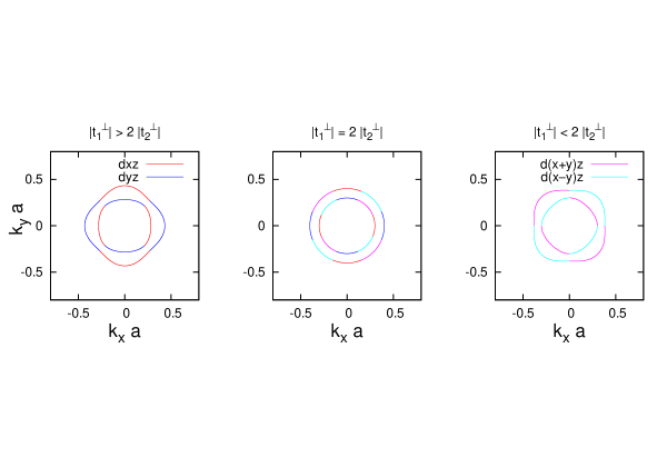
Figure 2: Shown are the hole Fermi surfaces centered at zero 2D momentum: $t_{\parallel}<0$. The concentration of holes is universally set to $x=0.01$, while the hopping matrix elements from left to right are (a) $t_{\perp}=0.40\,t_{\parallel}$ and $t_{\perp}^{\prime}=0.23\,t_{\parallel}$ , (b) $t_{\perp}=0.28\,t_{\parallel}$ and $t_{\perp}^{\prime}=0.28\,t_{\parallel}$ , and (c) $t_{\perp}=0.23\,t_{\parallel}$ and $t_{\perp}^{\prime}=0.40\,t_{\parallel}$ . Above, orbital labels are only approximate near the points on the Fermi surfaces at which they change.

To proceed further, we shall assume that both inter-orbital mean fields for Schwinger bosons $R_{1}^{\perp}$ and $R_{2}^{\perp}$ are real and positive. This will also be confirmed self-consistently. The slave-fermion matrix elements are then approximated by

$$\varepsilon_{\parallel}({\bi k})= \varepsilon_{\parallel}(0)-t_{\parallel}|{\bi k}|^{2}a^{2}$$ (3desacaja)

$$\varepsilon_{\perp}({\bi k})= -[t_{\perp}\cos(2\phi)+it_{\perp}^{\prime}\sin(2\phi)]|{\bi k}|^{2}a^{2}$$ (3desacajb)

for ${\bi k}$ near zero, where $t_{\parallel}=2t_{1}^{\parallel}Q_{1}^{\parallel}+4t_{2}^{\parallel}Q_{2}^{\parallel}$, where $t_{\perp}=2t_{1}^{\perp}({\hat{\bi x}})R_{1}^{\perp}$, and where $t_{\perp}^{\prime}=4t_{2}^{\perp}({\hat{\bi x}}+{\hat{\bi y}})R_{2}^{\perp}/i$ are real hopping amplitudes. Above, $\phi$ denotes the angle that ${\bi k}$ makes with $x$ axis. Henceforth, we shall assume hole bands: $t_{\parallel}<0$. The constant energy contours $\epsilon_{F}=\varepsilon_{\parallel}({\bi k})\pm|\varepsilon_{\perp}({\bi k})|$ then yield Fermi surfaces

$$k_{F\pm}^{2}(\phi)a^{2}=\epsilon_{F}^{\prime}/(-t_{\parallel}\pm[t_{\perp}^{2}\cos^{2}(2\phi)+t_{\perp}^{\prime 2}\sin^{2}(2\phi)]^{1/2})$$ (3desacajak)

at low doping $x\ll 1$, where $\epsilon_{F}^{\prime}=\epsilon_{F}-\varepsilon_{\parallel}(0)$. These are shown in Fig. 2. The average of the volume of phase space contained by the inner ($+$) Fermi surface and the outer ($-$) Fermi surface gives the hole concentration per orbital: $x=(2\pi)^{-2}\int_{0}^{2\pi}d\phi\sum_{\pm}\int_{0}^{k_{F\pm}(\phi)}dk\,k\,a^{2}/2$. The resulting angle integral is obtained by applying the residue theorem after making the change of variable $z=e^{4i\phi}$, which yields the relationship

$$4\pi x=\epsilon_{F}^{\prime}(-t_{\parallel})/(t_{\parallel}^{2}-t_{\perp}^{2})^{1/2}(t_{\parallel}^{2}-t_{\perp}^{\prime 2})^{1/2}$$ (3desacajal)

between the Fermi energy and the concentration of mobile holes. Next, the intra-orbital hopping fields for slave fermions are given by $P_{n}^{\parallel}=(2\pi)^{-2}\int_{0}^{2\pi}d\phi\sum_{\pm}\int_{0}^{k_{F\pm}(\phi)}dk\,k\,(1-{n\over 4}k^{2}a^{2})\,a^{2}/4$ at $x\ll 1$. Performing the angle integral after the previous change of variable yields the result

$$P_{n}^{\parallel}={1\over 2}x-{n\pi\over 4}x^{2}{t_{\parallel}^{2}-t_{\perp}^{2}t_{\perp}^{\prime 2}/t_{\parallel}^{2}\over{(t_{\parallel}^{2}-t_{\perp}^{2})^{1/2}(t_{\parallel}^{2}-t_{\perp}^{\prime 2})^{1/2}}}$$ (3desacajam)

for these amplitudes. Last, the mean fields for inter-orbital hopping by slave fermions are given by $P_{1}^{\perp}(\hat{\bi x})=(2\pi)^{-2}\int_{0}^{2\pi}d\phi\sum_{\pm}\int_{0}^{k_{F\pm}(\phi)}dk\,k^{3}\,(\mp\cos\,2\phi)e^{2i\delta_{f}({\bi k})}\,a^{4}/16$ and by $P_{2}^{\perp}(\hat{\bi x}+\hat{\bi y})=(2\pi)^{-2}\int_{0}^{2\pi}d\phi\sum_{\pm}\int_{0}^{k_{F\pm}(\phi)}dk\,k^{3}\,(\mp\sin\,2\phi)e^{2i\delta_{f}({\bi k})}\,a^{4}/8$ at low hole concentrations, where

$$e^{2i\delta_{f}({\bi k})}=-{t_{\perp}\cos(2\phi)+it_{\perp}^{\prime}\sin(2\phi)\over{[t_{\perp}^{2}\cos^{2}(2\phi)+t_{\perp}^{\prime 2}\sin^{2}(2\phi)]^{1/2}}}$$ (3desacajan)

is the fermion phase factor at ${\bi k}$ near zero. Employing again the change of variable $z=e^{4i\phi}$ in the resulting angle integrals then yields the following expressions for these amplitudes:

$$P_{1}^{\perp}(\hat{\bi x})={\pi\over 4}x^{2}{t_{\perp}\over{t_{\parallel}}}\Biggl{(}{t_{\parallel}^{2}-t_{\perp}^{\prime 2}\over{t_{\parallel}^{2}-t_{\perp}^{2}}}\Biggr{)}^{1/2},$$ (3desacajao)

$$P_{2}^{\perp}(\hat{\bi x}+\hat{\bi y})=i{\pi\over 2}x^{2}{t_{\perp}^{\prime}\over{t_{\parallel}}}\Biggl{(}{t_{\parallel}^{2}-t_{\perp}^{2}\over{t_{\parallel}^{2}-t_{\perp}^{\prime 2}}}\Biggr{)}^{1/2}.$$ (3desacajap)

Substitution into the expression for the inter-orbital matrix element experienced by Schwinger bosons (3desacai) reduces it to

$$\Omega_{\perp}^{\prime}({\bi k})=\pi x^{2}R_{1}^{\perp}{|2t_{1}^{\perp}|^{2}\over{t_{\parallel}}}\Biggl{(}{t_{\parallel}^{2}-t_{\perp}^{\prime 2}\over{t_{\parallel}^{2}-t_{\perp}^{2}}}\Biggr{)}^{1/2}\gamma_{1}({\bi k})+\pi x^{2}R_{2}^{\perp}{|4t_{2}^{\perp}|^{2}\over{t_{\parallel}}}\Biggl{(}{t_{\parallel}^{2}-t_{\perp}^{2}\over{t_{\parallel}^{2}-t_{\perp}^{\prime 2}}}\Biggr{)}^{1/2}\gamma_{2}({\bi k}).$$

(3desacajaq)

Observe that the phase factor associated with Schwinger bosons is then $e^{2i\delta_{b}({\bi k})}={\rm sgn}\,t_{\parallel}=-1$ near ${\bi k}=0$. The principal mean-field equation (3desab) implies ideal Bose-Einstein condensation (BEC) of the Schwinger bosons into the bottom of the spectrum (3desx) at $3$-momentum $(k_{0},{\bi k})=(\pi,0)$ in the zero-temperature limit. Comparison of (3desab) with the mean-field equations (3desaca) and (3desacb) yields the mean-field values $Q_{n}^{\parallel}=s_{0}$ and $Q_{n}^{\perp}=s_{1}$, in the large-$s_{0}$ limit, where $s_{1}=s_{0}\tanh\,2\theta=s_{0}[\Omega_{\perp}(0)/\Omega_{\parallel}(0)]$. Ideal BEC necessarily requires $\omega_{b}(\pi,0)=0$. This yields ultimately that $\tanh\,2\theta=(1+[\Omega_{\perp}^{\prime}(0)/\Omega_{\perp}(0)]^{2})^{-1/2}$. Inter-orbital hopping therefore diminishes the antiferromagnetic order in the hidden half-metal state: $s_{1}<s_{0}$. Notice, however, that the correction is small and of order $x^{4}$. Last, ideal BEC implies a unique mean-field amplitude $R_{n}^{\perp}=s_{2}$ by meanfield equations (3desacad), where $s_{2}=s_{0}\,{\rm sech}\,2\theta$, with ${\rm sech}\,2\theta=[|\Omega_{\perp}^{\prime}(0)|/\Omega_{\perp}(0)]/(1+[\Omega_{\perp}^{\prime}(0)/\Omega_{\perp}(0)]^{2})^{1/2}$. Observe now that the latter ratio of frequencies takes the form $|\Omega_{\perp}^{\prime}(0)|/\Omega_{\perp}(0)=A_{0}(s_{2}/s_{0}s_{1})$ as $x\rightarrow 0$, in which case $s_{1}\rightarrow s_{0}$. Here, $A_{0}$ is a positive constant that is small compared to unity at low hole concentration. Substituting this form into the previous definition of $s_{2}$ yields only the trivial solution $s_{2}=0$. We therefore conclude that inter-orbital hopping is dynamically suppressed in the present Schwinger-boson-slave-fermion mean-field theory for the hidden half-metal state at large electron spin $s_{0}$ and low hole concentration. In particular, Eqs. (3desacajao) and (3desacajap) imply that all of the inter-orbital mean fields, $P_{n}^{\perp}$ and $R_{n}^{\perp}$, are null.

Dynamical suppression of inter-orbital hopping at large-$s_{0}$ implies a null inter-orbital hopping matrix element for Schwinger bosons by Eq. (3desacajaq): $\Omega_{\perp}^{\prime}({\bi k})=0$. Inspection of the spectrum for Schwinger bosons (3desx) then yields the dispersion relation

$$\omega_{b}(k_{0},{\bi k})=v_{0}|{\bi k}|\quad{\rm near}\quad{\bi k}=0$$ (3desacajar)

at the zero-temperature limit, where

$$v_{0}=2s_{0}a(1-x)^{2}([J_{1}^{\perp}-{\bar{J}}_{1}^{\parallel}(x)+2J_{2}^{\perp}-2{\bar{J}}_{2}^{\parallel}(x)]\cdot[{1\over 2}J_{0}+2J_{1}^{\perp}+2J_{2}^{\perp}])^{1/2}$$ (3desacajas)

is the velocity of hidden spinwaves, with ${\bar{J}}_{n}^{\parallel}(x)=J_{n}^{\parallel}+(1-x)^{-2}s_{0}^{-1}t_{n}^{\parallel}x$ for $n=1,2$. At ${\bi k}$ near cSDW wavenumbers $(\pi/a)\hat{\bi x}$ and $(\pi/a)\hat{\bi y}$, the spectrum for Schwinger bosons (3desx) disperses anisotropically as

$$\omega_{b}(k_{0},{\bi k})=[\Delta_{cSDW}^{2}+v_{l}^{2}(k_{l}-\pi/a)^{2}+v_{t}^{2}k_{t}^{2}]^{1/2}$$ (3desacajat)

in the zero-temperature limit, with a spin gap

$$\Delta_{cSDW}=(1-x)^{2}(2s_{0})[(4J_{2}^{\perp}-J_{0c})(J_{0}-J_{0c})]^{1/2}$$ (3desacajau)

that vanishes at a critical Hund’s Rule coupling

$$-J_{0c}=2(J_{1}^{\perp}-J_{1}^{\parallel})-4J_{2}^{\parallel}-(1-x)^{-2}s_{0}^{-1}2t_{\parallel}x.$$ (3desacajav)

Above, $k_{l}$ and $k_{t}$ denote the longitudinal and transverse components of ${\bi k}$ with respect to the cSDW momentum. At criticality, $\Delta_{cSDW}=0$, the longitudinal spinwave velocity $v_{l}$ coincides with the hidden spinwave velocity $v_{0}$, while the anisotropy parameter is given by

$${v_{l}\over{v_{t}}}=\Biggl{[}{2{\bar{J}}_{2}^{\parallel}(x)+2J_{2}^{\perp}+{\bar{J}}_{1}^{\parallel}(x)+J_{1}^{\perp}\over{2{\bar{J}}_{2}^{\parallel}(x)+2J_{2}^{\perp}-{\bar{J}}_{1}^{\parallel}(x)-J_{1}^{\perp}}}\Biggr{]}^{1/2},$$ (3desacajaw)

which is greater than unity. The hidden half metal is stable at weak to moderate Hund’s Rule coupling $-J_{0}<-J_{0c}$. Equation (3desacajav) therefore implies that intra-orbital hole hopping stabilizes the hidden half-metal state for hole bands, $t_{\parallel}<0$. (See Fig. 1.) We conclude that the hidden half metal is robust with respect to the presence of inter-orbital hopping within the present Schwinger-boson-slave-fermion mean-field theory.

Finally, returning to the generic unoptimized mean-field theory, the inversion of the similarity transform (3desy) yields slave-fermion states that are annihilated by

$$f(k_{0},{\bi k})={e^{+i\delta_{f}({\bi k})}\over{2^{1/2}}}f_{d-}({\bi k})+e^{ik_{0}}{e^{-i\delta_{f}({\bi k})}\over{2^{1/2}}}f_{d+}({\bi k}).$$ (3desacajax)

Their corresponding Wannier wave functions then depend on the azimuthal angle $\phi^{\prime}$ about each iron atom as $\cos[\phi^{\prime}-\delta_{f}({\bi k})]$ in the even channel, $k_{0}=0$, and as $\sin[\phi^{\prime}-\delta_{f}({\bi k})]$ in the odd channel, $k_{0}=\pi$. Figure 2 depicts slave-fermion Fermi surfaces (3desacajak) at low doping $x=0.01$. Dynamical suppression of inter-orbital hopping implies that the matrix element for inter-orbital hopping of slave fermions (3der) is null, however. The inner and outer Fermi surface hole pockets depicted by Fig. 2 must therefore collapse into two degenerate circular Fermi surface hole pockets at low doping, $x\ll 1$, at large spin $s_{0}$. We believe that this effect is due to the inability of the two-orbital $t$-$J$ model (LABEL:tJ) to “erase” strings of overturned spins that result from inter-orbital hole hopping in the classical limit, at large spin $s_{0}$[34][35]. Related behavior is predicted theoretically for a mobile hole in the Néel state over the one-orbital square lattice, where nearest-neighbor hopping ($t_{1}$) is dynamically suppressed at low energy, leaving effective next-nearest-neighbor hopping ($t_{2}$) within the same antiferromagnetic sublattice[39][40][41]. As we will see in section 4, this limiting result persists for true electron spin $s_{0}=1/2$ in a special case.

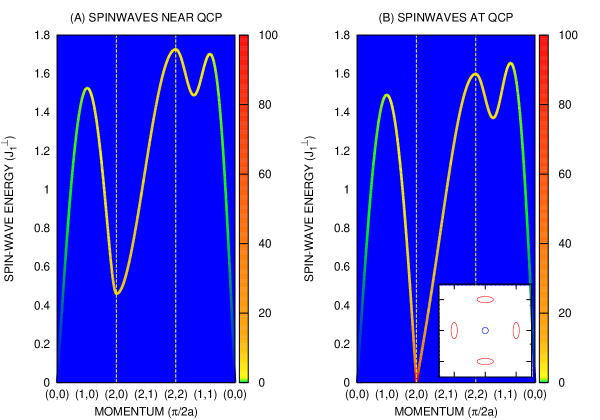
Figure 3: The mean-field result for the imaginary part of the dynamical spin response function in the zero-temperature-large-$s_{0}$ limit, Eqs. (3desacajba) and (3desacajbb), is evaluated with the following set of parameters: $J_{1}^{\parallel}=0$, $J_{1}^{\perp}>0$, $J_{2}^{\parallel}=0.3\,J_{1}^{\perp}=J_{2}^{\perp}$, $t_{1}^{\parallel}=-5J_{1}^{\perp}$, $t_{2}^{\parallel}=0$, $x=0.01$, and $s_{0}=1/2$. Dynamical suppression of inter-orbital hopping is presumed. The Hund’s Rule coupling is set to $-J_{0}=-J_{0c}-0.1J_{1}^{\perp}$ just off the QCP in panel (A), while it is set to the critical value $-J_{0c}$ in panel (B). Low-energy contours are displayed in the inset.

3.2 Spinwaves

We shall now determine the spin excitations of the hidden half metal by directly computing the dynamical spin-spin correlation function from the Schwinger-boson-slave-fermion mean-field theory. First, we identify the true $(k_{0}=0)$ versus the hidden $(k_{0}=\pi)$ spin at each iron atom $i$: ${\bi S}_{i}(k_{0})={\bi S}_{i,d-}+e^{ik_{0}}{\bi S}_{i,d+}$. Consider then the transverse dynamical spin-spin correlation function $\langle{\bi S}(k_{0})\cdot{\bi S}^{\prime}(k_{0})\rangle|^{\perp}={1\over 2}\langle S^{+}(k_{0})S^{\prime-}(k_{0})+S^{-}(k_{0})S^{\prime+}(k_{0})\rangle$ at space-time points $({\bi r},t)$ and $({\bi r}^{\prime},t^{\prime})$. Averaging the slave-fermion dynamics over the bulk, we obtain the form

$$\langle{\bi S}(k_{0})\cdot{\bi S}^{\prime}(k_{0})\rangle|^{\perp}_{{\bi k},\omega}=(1-x)^{2}{\hbar^{2}\over 2} \sum_{\alpha=0,1}\sum_{\beta=0,1}e^{ik_{0}(\alpha-\beta)}\cdot$$ (3desacajay)

$$\cdot[G_{\alpha,\beta}^{(b)}*G_{\alpha,\beta}^{(b)*}+F_{\alpha,\beta}^{(b)}*F_{\alpha,\beta}^{(b)*}]|_{{\bi k},\omega},$$

for its Fourier transform, where $iG_{\alpha,\beta}^{(b)}({\bi r}_{i},t;{\bi r}_{j},t^{\prime})=\langle b_{i,\alpha,s}(t)b_{j,\beta,s}^{\dagger}(t^{\prime})\rangle$ and $iF_{\alpha,\beta}^{(b)}({\bi r}_{i},t;{\bi r}_{j},t^{\prime})=\langle b_{i,\alpha,s}(t)b_{j,\beta,\bar{s}}(t^{\prime})\rangle$ are the regular and the anomalous Greens functions for the Schwinger bosons, and where the notation $f*g$ denotes a convolution in frequency and momentum. Above, we use the index $0$ and $1$ for the orbitals $d-$ and $d+$. Also, henceforth in this subsection, we shall identify $k_{0}=0$ and $\pi$ with the respective labels $+$ and $-$. After substitution of the Bogoliubov transformation (3desa,$b$) and of the similarity transform (3desv), a standard summation of the Matsubara frequencies in the convolution yields the following Auerbach-Arovas expression for the dynamical spin correlator at $T>0$ [42]:

$$i\langle{\bi S}(\pm)\cdot{\bi S}^{\prime}(\pm)\rangle|^{\perp}_{{\bi k},\omega}={\hbar^{2}\over 4}{(1-x)^{2}\over{\cal N}} \sum_{q_{0}=+,-}\sum_{\bi q}\Biggl{\{}(1+\cosh\,[2\theta({\bi q})\mp 2\theta({\bi q}-{\bi k})])\cdot$$

$$\cdot\sum_{\nu=-\omega,+\omega}{n_{B}[\omega_{b}(q_{0},{\bi q})]-n_{B}[\omega_{b}(q_{0}\pm,{\bi q}-{\bi k})]\over{\nu-\omega_{b}(q_{0},{\bi q})+\omega_{b}(q_{0}\pm,{\bi q}-{\bi k})}}+$$

$$+(1-[\cosh\,2\theta({\bi q})][\cosh\,2\theta({\bi q}-{\bi k})])\cdot$$

$$\cdot\sum_{\nu=-\omega,+\omega}{n_{B}[\omega_{b}(q_{0},{\bi q})]+n_{B}[\omega_{b}(q_{0}\pm,{\bi q}-{\bi k})]\over{\nu-\omega_{b}(q_{0},{\bi q})-\omega_{b}(q_{0}\pm,{\bi q}-{\bi k})}}+$$

$$\pm[\sinh\,2\theta({\bi q})][\sinh\,2\theta({\bi q}-{\bi k})]\cdot$$

$$\cdot\sum_{\nu=-\omega,+\omega}{n_{B}[\omega_{b}(q_{0},{\bi q})]+n_{B}[\omega_{b}(q_{0}\mp,{\bi q}-{\bi k})]\over{\nu-\omega_{b}(q_{0},{\bi q})-\omega_{b}(q_{0}\mp,{\bi q}-{\bi k})}}\Biggr{\}}.$$

When computing $q_{0}\pm$ above, we use the multiplication table $\pm\pm=+$ and $\mp\pm=-$. The property $\omega_{b}(q_{0},{\bi q})=\omega_{b}(q_{0},-{\bi q})$ displayed by the spectrum for Schwinger bosons (3desx) was exploited to obtain the reduced expression (LABEL:AA). Expression (LABEL:AA) can be used to show that $(2\pi)^{-1}\int_{-\infty}^{+\infty}d\omega\langle{\bi S}(+)\cdot{\bi S}^{\prime}(+)\rangle|^{\perp}_{{\bi k},\omega}=0$ at ${\bi k}=0$. This is consistent with a spin-singlet hidden-order antiferromagnetic state inside the subspace where $\sum_{i}\sum_{\alpha}S_{z,i,\alpha}=0$: $\langle|\sum_{i}\sum_{\alpha}{\bi S}_{i,\alpha}|^{2}\rangle=0$.

At large electron spin $s_{0}$, the true self-consistent mean-field theory dynamically suppresses inter-orbital hopping, however. This leads to Schwinger bosons with degenerate spectra: $\omega_{b}(q_{0},{\bi k})=\omega_{b}^{(0)}({\bi k})$ for $q_{0}=+,-$. At zero temperature, expression (LABEL:AA) in conjunction with ideal BEC then yields the result[21]

$$i\langle{\bi S}(\pm)\cdot{\bi S}^{\prime}(\pm)\rangle|^{\perp}_{{\bi k},\omega}=\pi^{-1}A(\pm,{\bi k})([\omega_{b}^{(0)}({\bi k})-\omega]^{-1}+[\omega_{b}^{(0)}({\bi k})+\omega]^{-1}),$$ (3desacajba)

where the poles in frequency have spectral weight

$$A(\pm,{\bi k})=\pi(1-x)^{2}s_{0}\hbar^{2}[\Omega_{\mp}({\bi k})/\Omega_{\pm}({\bi k})]^{1/2}.$$ (3desacajbb)

Here, $\Omega_{\pm}=\Omega_{\parallel}\pm\Omega_{\perp}$. The above dynamical spin correlator coincides with the transverse spin susceptibility, $\chi_{\perp}(k,\omega)$, in the present zero-temperature limit by the fluctuation-dissipation theorem. Notice that the spectral weights (3desacajbb) above diverge at $\Omega_{\pm}({\bi k})=0$. This implies the existence of hidden $(-)$ spin waves near zero 2D momentum with a spectrum (3desacajar), as well as true $(+)$ spin waves near cSDW momenta with a spectrum (3desacajat) [21]. We conclude that the hidden half-metal state shows strict long-range antiferromagnetic order across the $d+$ and $d-$ orbitals of the iron atoms at zero temperature.

The true spin excitations $(+)$ predicted by the dynamical spin susceptibility (3desacajba) near the quantum-critical point are shown graphically by Fig. 3 for a set of parameters that is applicable to iron-pnictide high-temperature superconductors. Notice the spin gap (3desacajau) that exists at cSDW wavenumbers $(\pi/a){\hat{\bi x}}$ and $(\pi/a){\hat{\bi y}}$. It collapses to zero at a critical Hund’s Rule coupling (3desacajav) of moderate strength. This suggests that the hidden half-metal state gives way to a cSDW metal phase[43] that shows long-range cSDW correlations at the QCP, which separates the two phases.

3.3 Fermi Surfaces

We shall now obtain the electronic structure of the hidden half-metal state by computing the one-electron propagator directly from the Schwinger-boson-slave-fermion mean-field theory for the two-orbital $t$-$J$ model. It is given by the convolution of the propagator for Schwinger bosons with the propagator for slave fermions: $iG({\bi k},\omega)=\sum_{\alpha=d-,d+}G_{\alpha,\alpha}^{(b)}*G_{\alpha,\alpha}^{(f)*}|_{{\bi k},\omega}$, where $iG_{\alpha,\beta}^{(f)}({\bi r}_{i},t;{\bi r}_{j},t^{\prime})=\langle f_{i,\alpha}(t)f_{j,\beta}^{\dagger}(t^{\prime})\rangle$. A standard summation of Matsubara frequencies yields the expression[21]

$$G({\bi k},\omega)=\sum_{k_{0}=0,\pi}{1\over{\cal N}}\sum_{q} \Biggl{(}[\cosh\,\theta({\bi q})]^{2}{{n_{B}[\omega_{b}(q)]+n_{F}[\varepsilon_{f}(q-k)]}\over{\omega-\omega_{b}(q)+\varepsilon_{f}(q-k)}}+$$ (3desacajbc)

$$+[\sinh\,\theta({\bi q})]^{2}{{n_{B}[\omega_{b}(q)]+{\bar{n}}_{F}[\varepsilon_{f}(q-k)]}\over{\omega+\omega_{b}(q)+\varepsilon_{f}(q-k)}}\Biggr{)}.$$

Above, ${\bar{n}}_{F}(\varepsilon)=({\rm exp}[(\mu-\varepsilon)/k_{B}T]+1)^{-1}$. All of the Schwinger bosons condense into the lowest-energy state at $3$-momentum $(q_{0},{\bi q})=(\pi,0)$ as $T\rightarrow 0$ by the principal meanfield equation (3desab). This results in the following coherent contribution to the electronic spectral function at zero temperature and at large $s_{0}$:

$${\rm Im}\,G_{\rm coh}({\bi k},\omega)=s_{0}{\pi}\sum_{k_{0}=0,\pi}\delta[\omega+\varepsilon_{f}(k_{0},{\bi k})].$$ (3desacajbd)

In the case of the unoptimized generic mean-field theory, it reveals inner and outer hole Fermi surfaces centered at zero 2D momentum that are depicted by Fig. 2. These collapse into doubly-degenerate circular hole pockets in the self-consistent mean-field theory at large $s_{0}$, where inter-orbital hopping is dynamically suppressed.

The contribution due to the Fermi-Dirac terms in the above expression (3desacajbc) represent incoherent excitations in the electronic structure. At energies $\omega$ below the electronic Fermi level, the pole in the second term of expression (3desacajbc) represents the combination of a hole excitation, $\varepsilon_{f}>\mu$, with a spinwave, $\omega_{b}>0$. This composite excitation therefore shows a gap (3desacajau) about cSDW momenta, $\Delta_{cSDW}$. Notice that copies of the previous inner and outer Fermi surfaces now centered at cSDW wavenumbers $(\pi/a){\hat{\bi x}}$ and $(\pi/a){\hat{\bi y}}$ exist at the QCP because of the collapse of the spin gap there: $\Delta_{cSDW}\rightarrow 0$. (See Fig. 3.) This is a spin-density wave nesting mechanism in reverse, where low-energy spinwaves centered at cSDW momenta produce nested Fermi surfaces. The incoherent contribution due to the first term in expression (3desacajbc) above vanishes in the zero-temperature limit at energies $\omega$ below the electronic Fermi level. Detailed evaluations of ${\rm Im}\,G_{\rm inc}({\bi k},\omega)$ from the Fermi-Dirac terms in expression (3desacajbc) find electron-type dispersion for the emergent band at momenta that lie inside of the nested Fermi surface pocket[21]. They also find hole-type dispersion of the emergent band at momenta that lie outside of the nested Fermi surface[21], however. We believe that the latter is an artifact of the present mean-field approximation. Indeed, strong arguments for electron-type emergent bands will be presented at the end of section 5.

To conclude, Schwinger-boson-slave-fermion meanfield theory of the two-orbital $t$-$J$ model (LABEL:tJ) at a quantum-critical point predicts nested Fermi surfaces centered at zero 2D momentum and at cSDW momenta that are circular in shape. The Fermi surface pockets centered at cSDW momenta have purely $3d_{xz}$ and $3d_{yz}$ orbital character by construction, which is consistent with a recent ARPES study of the electronic structure in optimally doped Ba(Fe_1-xCo_x)₂As₂ [5].

4 Exact Diagonalization

The previous Schwinger-boson-slave-fermion meanfield theory for the two-orbital $t$-$J$ model (LABEL:tJ) predicts that electronic structure centered at cSDW momenta emerges at a quantum critical point that separates a cSDW metal from a hidden half-metal state. This result was obtained in the limit of large electron spin $s_{0}$. Below, we will see that the effect persists for true electron spin, $s_{0}=1/2$.

We have obtained the exact low-energy spectrum of the two-orbital $t$-$J$ model (LABEL:tJ) for $4\times 4\times 2$ local spin-$1/2$ moments plus one mobile hole by computer calculation. The Schwinger-boson-slave-fermion representation (3deh) of the correlated electron is applied exactly. In particular, a quantum state is specified by the combination of an arbitrary spin background over all of the $4\times 4\times 2$ sites, confined to the subspace with total spin $S_{z}=0$, and a hole location at one of the down-spin sites in the given spin background. The Heisenberg-exchange and Hund-exchange terms in the $t$-$J$ model Hamiltonian (LABEL:tJ) reduce to permutations of the spin backgrounds, and these are stored in memory. The matrix elements for correlated hopping terms in (LABEL:tJ) are computed directly at each application of the Hamiltonian operator, on the other hand. Periodic boundary conditions are imposed, and translation and reflection symmetries on the $4\times 4\times 2$ lattice are exploited in order to reduce the dimension of the Hilbert space. Global swap of the orbitals, $P_{d\bar{d}}$, is included in the list of symmetry operations at the extreme where inter-orbital next-nearest-neighbor hopping is suppressed: $t_{2}^{\perp}=0$. For example, exploiting reflections about both principal axes of the $4\times 4$ square lattice of iron atoms plus $P_{d\bar{d}}$ brings the dimension of the Hilbert space down to 75,624,211 states in such case at zero-momentum and even reflection parities. The low-energy states of the resulting block-diagonal Hamiltonian are obtained by employing the Lanczos technique[44]. We use the ARPACK subroutine library for this purpose[45], in which case the Hamiltonian operation $|\psi^{\prime}\rangle=H|\psi\rangle$ is accelerated by exploiting parallel threads with OpenMP directives.

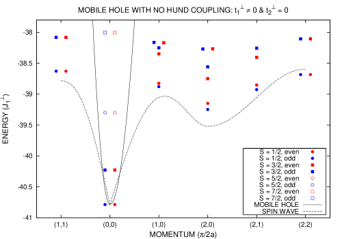
Figure 4: Shown is the low-energy spectrum of the two-orbital $t$-$J$ model, Eq. (LABEL:tJ), over a $4\times 4\times 2$ lattice with one hole, in the absence of Hund’s Rule: $J_{0}=0$. The remaining parameters are $J_{1}^{\parallel}=0$, $J_{1}^{\perp}>0$, $J_{2}^{\parallel}=0.3J_{1}^{\perp}=J_{2}^{\perp}$, $t_{1}^{\parallel}=-5J_{1}^{\perp}$, $t_{1}^{\perp}({\hat{\bi x}})=-2J_{1}^{\perp}$, $t_{1}^{\perp}({\hat{\bi y}})=+2J_{1}^{\perp}$, and $t_{2}^{\parallel}=0=t_{2}^{\perp}$. Red and blue states are respectively even and odd under $P_{d\bar{d}}$. Henceforth, some points on the spectrum are artificially moved slightly off their quantized values along the momentum axis for the sake of clarity. A comparison with the hole spectrum, $\varepsilon_{f}(k)=\varepsilon_{\parallel}({\bi k})$, and with the spin-wave spectrum, $\omega_{b}(k)=\omega_{b}^{(0)}({\bi k})$, at large $s_{0}$ and $x=0$ is also shown.

Figures 4, 5 and 7 display the evolution of the low-energy spectrum of one mobile hole in a $4\times 4$ lattice of spin-$1$ iron atoms with the strength of the Hund’s Rule coupling, $-J_{0}$. We chose the following set of Heisenberg exchange coupling constants and hopping matrix elements: $J_{1}^{\parallel}=0$, $J_{1}^{\perp}>0$, $J_{2}^{\parallel}=0.3J_{1}^{\perp}=J_{2}^{\perp}$, $t_{1}^{\parallel}=-5J_{1}^{\perp}$, $t_{1}^{\perp}({\hat{\bi x}})=-2J_{1}^{\perp}$, $t_{1}^{\perp}({\hat{\bi y}})=+2J_{1}^{\perp}$, and $t_{2}^{\parallel}=0=t_{2}^{\perp}$. Recall that global swap of the orbitals, $P_{d\bar{d}}$, is then an exact symmetry. (See the end of section 2.) Also, the mean-field result (3desacajav) then predicts a quantum critical point at $J_{0}=-0.8J_{1}^{\perp}$ in the thermodynamic limit $(x=0)$. It separates a hidden half-metal state at weak Hund’s Rule coupling from a cSDW at strong Hund’s Rule coupling. Figure 4 displays the exact spectrum in the absence of Hund’s Rule. Red and blue points denote states that are respectively even and odd under $P_{d\bar{d}}$. The spectrum is consistent with a hidden half metal. In particular, the lowest-energy states at fixed momentum carry spin-$1/2$ and they are nearly doubly degenerate. Furthermore, the pairs of spin-$1/2$ states in Fig. 4 are close in energy to the next-excited pairs of states at fixed momentum, which carry spin-$3/2$. By the summation of angular momentum, these two pairs of states can be understood as the combination of a well-defined spin-$1/2$ hole excitation and a well-defined spin-$1$ excitation that interact weakly. The pole in the second term of the one-electron propagator (3desacajbc) obtained by the previous Schwinger-boson-slave-fermion meanfield theory for the hidden half-metal state suggests that the energy dispersion relation of one hole of momentum ${\bi q}$ is equal to $\varepsilon_{f}(0)+\omega_{b}^{(0)}({\bi q})$ at $v_{0}/a\ll-t_{\parallel}$. In other words, the momentum of one hole is carried entirely by the spinwave that accompanies it. Figure 4 shows that the dispersion of the pairs of spin-$1/2$ and spin-$3/2$ low-energy states follows rather closely the trend set by the spin-wave dispersion $\omega_{b}^{(0)}({\bi q})$. (See also Fig. 9.) In particular, the mean-field result sets a lower bound for the exact dispersion of one hole in the two-orbital $t$-$J$ model (LABEL:tJ). This is very likely due to the larger Hilbert space of the Schwinger-boson-slave-fermion mean-field theory, which only enforces the constraint against double occupancy (3deh) on average over the bulk.

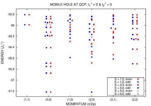
Figure 5: The low-energy spectrum of the two-orbital $t$-$J$ model with one hole roaming over a $4\times 4\times 2$ lattice is displayed at the QCP that separates the cSDW from the hidden half-metal state: $J_{0c}=-1.733J_{1}^{\perp}$. The remaining set of parameters are listed in the caption to Fig. 4. Red and blue states are respectively even and odd under $P_{d\bar{d}}$.

Table 1: Listed are groundstate expectation values of physical observables for one hole hopping over a $4\times 4\times 2$ lattice with the set of $t$-$J$ model parameters that are used in Figs. 4-7: $t_{1}^{\perp}\neq 0$ and $t_{2}^{\perp}=0$. Below, the QCP occurs at $J_{0c}=-1.733J_{1}^{\perp}$, and the integer coordinates $(n_{x},n_{y})$ specify the momentum of the groundstate in units of $\pi/2a$. And in the case of a doubly degenerate groundstate, relationships between the signs of $\langle P_{d\bar{d}}\rangle$ and of $\langle P_{d\bar{d}}(\circ)\rangle$ are specified by the $\pm$ and $\mp$ symbols.

• Observable	$J_{0}=0$ @ $(0,0)$	QCP @ $(0,0)$	QCP @ $(2,0)$	$J_{0}=-23J_{1}^{\perp}$ @ $(1,0)$
  Fe triplets	$7.90$	$11.50$	$13.48$	$14.96$
  $\mu_{\rm hFM}^{2}/\mu_{\rm Fe}^{2}$	$0.93$	$0.60$	0.26	$0.06$
  $\mu_{\rm cSDW}^{2}/\mu_{\rm Fe}^{2}$	$0.08$	$0.24$	$0.70$	$0.94$
  $P_{d\bar{d}}$	$\pm 1$	$\pm 1$	$-1$	$-1$
  $P_{d\bar{d}}(\circ)$	$\mp 0.06$	$\pm 0.02$	$-0.47$	$-0.94$

Figure 5 shows how the spin-$1/2$ state at cSDW wavenumber $(\pi/a){\hat{\bi x}}$, with odd parity under $P_{d\bar{d}}$, comes down in energy with increasing Hund’s Rule coupling to become degenerate with the zero-momentum doubly-degenerate groundstate at a critical coupling of $J_{0c}=-1.73J_{1}^{\perp}$. Turning off inter-orbital hopping entirely results in a somewhat higher critical Hund’s Rule coupling of[21] $J_{0c}=-2.27J_{1}^{\perp}$. We have measured the expectation value for local orbital swap at the hole iron site, $P_{d\bar{d}}(\circ)$. It has eigenvalues $+1$ and $-1$, which correspond to a hole with $3d_{xz}$ and with $3d_{yz}$ orbital character, respectively. Table 1 lists the corresponding expectation value over the groundstate at cSDW wavenumber $(\pi/a){\hat{\bi x}}$: $\langle P_{d\bar{d}}(\circ)\rangle=-0.47$. The emergent hole state therefore has $74\,\%$ $3d_{yz}$ orbital character. Also, the dispersion of the low-energy spin-$1/2$ states shown in Fig. 5 resembles the mean-field prediction for the dispersion of critical spin-wave excitations shown in Fig. 3. The former states are also well separated from the next excited state at fixed momentum. This again is consistent with the mean-field prediction (3desacajba) of well-defined spin-wave excitations at the QCP. Finally, the ordered moment for a hidden ferromagnet (hFM) and for a cSDW is defined by $\mbox{\boldmath$\mu$}(k)=[2\mu_{B}/(N_{\rm Fe}-{1\over 2})]\sum_{\alpha=0}^{1}\sum_{i}e^{i(k_{0}\alpha+{\bi k}\cdot{\bi r}_{i})}{\bi S}_{i,\alpha}$, with respective 3-momenta $k=(\pi,0,0)$ and $k=(0,\pi/a,0)$. Table 1 lists the auto-correlation of each over the groundstate at zero 2D momentum: $\langle\mbox{\boldmath$\mu$}(k)\cdot\mbox{\boldmath$\mu$}(-k)\rangle_{0}$. They are given in units of the ordered moment of the ferromagnetic state, $k=(0,0,0)$, over the $4\times 4\times 2$ lattice: $\mu_{\rm Fe}^{2}=(33/31)(2\mu_{B})^{2}$. Notice that $\mu_{cSDW}^{2}$ remains small at the QCP in the case of the zero-momentum groundstate, which is consistent with neutron diffraction studies in iron-pnictide systems[10]. Notice also that $\mu_{hFM}^{2}$ remains sizable at the quantum critical point for the zero-momentum groundstate, which indicates that hidden half-metal character persists there. Figure 6 displays the evolution of these ordered moments near the QCP. The QCP bisects the points at which $\mu_{hFM}^{2}$ and $\mu_{cSDW}^{2}$ dovetail for groundstates with 2D momenta at zero and at $(\pi/a)\hat{\bi x}$. Also displayed is the square of the moment $\mu(k)$ for Néel order, $k=(0,\pi/a,\pi/a)$, which always remains small. The large values of $\mu_{hFM}^{2}$ displayed by Fig. 6 at Hund coupling below critical in conjunction with the mean-field prediction, Eqs. (3desacajba) and (3desacajbb), argues strongly for the persistence of hidden ferromagnetic order in the thermodynamic limit. With the exception of the QCP, theoretical predictions for long-range cSDW order in the two-orbital $t$-$J$ model (LABEL:tJ) are absent, however. (Cf. section 5.) It is therefore unclear whether the cSDW order displayed by Fig. 6 at Hund coupling above critical survives the thermodynamic limit.

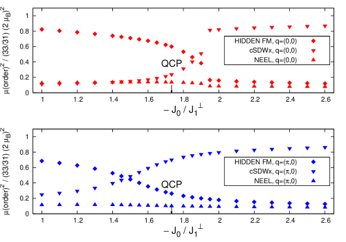
Figure 6: Shown is the evolution of the ordered moments about the QCP for the groundstate at zero (red) and at cSDW (blue) momenta. Model parameters are listed in the caption to Fig. 4. The ordered moments for the groundstate at zero 2D momentum (red) jump at $J_{0}=-1.95\,J_{1}^{\perp}$ because of a level crossing there between the spin-$1/2$ and spin-$3/2$ states. (See Fig. 12, left panel.)

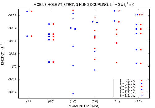
Figure 7: The low-energy spectrum of the two-orbital $t$-$J$ model with one mobile hole hopping over a $4\times 4\times 2$ lattice is displayed at strong Hund’s Rule coupling: $J_{0}=-23J_{1}^{\perp}$. The remaining parameters are listed in the caption to Fig. 4.

Last, Fig. 7 displays the exact low-energy spectrum for a $4\times 4$ lattice of true spin-$1$ iron atoms with one mobile hole. In particular, Hund’s Rule is enforced by setting $J_{0}=-23J_{1}^{\perp}$. As before, red points and blue points are even and odd under global orbital swap, $P_{d\bar{d}}$. We measured the expectation values for local orbital swap at the hole iron site, $P_{d\bar{d}}(\circ)$, and we found that the hole in even and odd parity states has orbital character that is over $95\,\%$ $3d_{xz}$ and $3d_{yz}$, respectively . (See Table 1.) We have therefore replaced the former labels with the latter ones in the legend to Fig. 7. The groundstate notably has spin-$1/2$, it carries momentum $(\pi/2a){\hat{\bi x}}({\hat{\bi y}})$, and it has orbital $3d_{yz}(3d_{xz})$ character. This is analogous to the groundstate momentum of $(\pi/2a)({\hat{\bi x}}\pm{\hat{\bi y}})$ that is predicted for one mobile hole in a 2D Néel state by Kane, Lee and Read[36]. Table 1 lists ordered moments computed in the groundstate at momentum $(\pi/2a){\hat{\bi x}}({\hat{\bi y}})$. These moments combined with the low-energy spectrum suggest that the groundstate at thermodynamic hole densities $x$ is a robust cSDW metal with Fermi surfaces that are centered at wavenumbers $(\pi/2a){\hat{\bi x}}$ and $(\pi/2a){\hat{\bi y}}$. This state is therefore unable to account for the Fermi surfaces that are observed experimentally in iron-pnictide systems.

Table 2: Listed are the characteristic properties of observable versus hidden quantum-critical spin-wave excitations in the two-orbital Heisenberg model that corresponds to the two-orbital $t$-$J$ model (LABEL:tJ) at half filling. (See ref. [14], Fig. 5.)

• spin wave	order parameter	2D momentum	Hund’s Rule?	$P_{d\bar{d}}$ & $P_{d\bar{d}}^{\prime}$
  observable	${\bi S}_{i,d-}+{\bi S}_{i,d+}$	$(\pi/a){\hat{\bi x}}({\hat{\bi y}})$	obeyed	even
  hidden	${\bi S}_{i,d-}-{\bi S}_{i,d+}$	zero	violated	odd

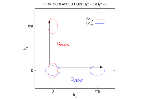
Figure 8: Emergent nesting of Fermi surface pockets at QCP with nearest-neighbor inter-orbital hopping: negative $t_{1}^{\perp}(\hat{\bi x})=-t_{1}^{\perp}(\hat{\bi y})$ and $t_{2}^{\perp}=0$. (Cf. figs. 2 and 5.)

Figure 6 provides evidence for a QCP that separates a cSDW metal from a hidden half metal as Hund coupling gets weaker. The exact quantum-critical spectrum displayed by Fig. 5 reveals groundstates at zero 2D momentum that are degenerate with groundstates at cSDW momenta $(\pi/a)\hat{\bi x}$ and $(\pi/a)\hat{\bi y}$. The expectation values for $\langle P_{d\bar{d}}(\circ)\rangle$ that are listed in Table 1 imply that the latter are emergent mobile hole states with $74\,\%$ $3d_{yz}$ and $74\,\%$ $3d_{xz}$ orbital character, respectively. Coherent inter-orbital hole propagation at cSDW wavelengths therefore exists at the QCP in the case where inter-orbital hopping is purely across nearest neighbors. This contrasts with the prediction of dynamical suppression of inter-orbital hopping by the previous Schwinger-boson-slave-fermion mean-field theory at large $s_{0}$. General agreement between the two calculations nevertheless exists. In particular, both the exact results shown by Fig. 5 and the previous Schwinger-boson-slave-fermion mean-field theory analysis find a QCP at moderate Hund’s Rule coupling, $-J_{0}$, where one-hole groundstates at zero 2D momentum and at cSDW momenta become degenerate. The mean-field theory predicts that the momentum of the degenerate groundstate in Fig. 5 is carried entirely by a cSDW spinwave that softens to zero excitation energy at the QCP. (See Fig. 3.) Table 2 summarizes the nature of quantum-critical spinwave excitations for the corresponding Heisenberg model in the absence of mobile holes[14]. The key point to notice is that quantum-critical spinwaves at cSDW momenta are observable, with even parity under $P_{d\bar{d}}$, while those at zero 2D momentum are hidden, with odd parity under $P_{d\bar{d}}$. [See Eqs. (3desacajba) and (3desacajbb), and Fig. 3.] We have confirmed this by exact diagonalization of the corresponding Heisenberg model. Combining the mean-field-theory picture of the QCP with the present exact results then leads to the following conjecture: the critical cSDW spinwave at wavenumber $(\pi/a){\hat{\bi x}}$ relates the odd parity $3d_{yz}$ portion of the hole pockets centered at zero 2D momentum (Fig. 2) with an emergent Fermi-surface pocket centered at $(\pi/a){\hat{\bi x}}$ that has the same orbital character, while the critical cSDW spinwave at wavenumber $(\pi/a){\hat{\bi y}}$ relates the even parity $3d_{xz}$ portion of the hole pockets centered at zero 2D momentum with an emergent Fermi-surface pocket centered at $(\pi/a){\hat{\bi y}}$ that has the same orbital character. Figure 8 summarizes this emergent nesting mechanism. Notice that Fermi surface pockets centered at cSDW momenta have orbital character that is purely $3d_{xz}$ and $3d_{yz}$, with no admixture of other $3d$ orbitals. This is consistent with a recent determination of the electronic structure in optimally doped Ba(Fe_1-xCo_x)₂As₂ by ARPES[5].

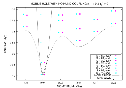
Figure 9: Shown is the low-energy spectrum of the two-orbital $t$-$J$ model, Eq. (LABEL:tJ), over a $4\times 4\times 2$ lattice with one hole, in the absence of Hund’s Rule: $J_{0}=0$. The remaining parameters are $J_{1}^{\parallel}=0$, $J_{1}^{\perp}>0$, $J_{2}^{\parallel}=0.3J_{1}^{\perp}=J_{2}^{\perp}$, $t_{1}^{\parallel}=-5J_{1}^{\perp}$, $t_{1}^{\perp}=0$, $t_{2}^{\parallel}=0$, $t_{2}^{\perp}({\hat{\bi x}}+{\hat{\bi y}})=-iJ_{1}^{\perp}$, and $t_{2}^{\perp}(-{\hat{\bi x}}+{\hat{\bi y}})=+iJ_{1}^{\perp}$. Pink and light blue states are respectively even and odd under $P_{d\bar{d}}^{\prime}$. A comparison with the hole spectrum, $\varepsilon_{f}(k)=\varepsilon_{\parallel}({\bi k})$, and with the spin-wave spectrum, $\omega_{b}(k)=\omega_{b}^{(0)}({\bi k})$, at large $s_{0}$ and $x=0$ is also shown.

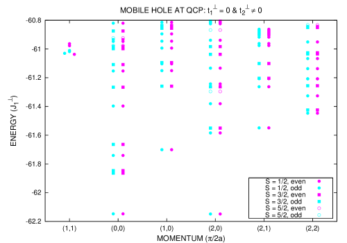
Figure 10: The low-energy spectrum of the two-orbital $t$-$J$ model with one hole roaming over a $4\times 4\times 2$ lattice is displayed at the QCP that separates the cSDW from the hidden half-metal state: $J_{0c}=-2.26J_{1}^{\perp}$. The remaining set of parameters are listed in the caption to the Fig. 9. Pink and light blue states are respectively even and odd under $P_{d\bar{d}}^{\prime}$.

Figures 9 and 10 show the exact spectrum of the two-orbital $t$-$J$ model (LABEL:tJ), respectively, in the absence of Hund’s Rule coupling and at the QCP, but at the other extreme where inter-orbital hopping is purely across next-nearest neighbors. The model parameters, in particular, are $J_{1}^{\parallel}=0$, $J_{1}^{\perp}>0$, $J_{2}^{\parallel}=0.3J_{1}^{\perp}=J_{2}^{\perp}$, $t_{1}^{\parallel}=-5J_{1}^{\perp}$, $t_{1}^{\perp}=0$, $t_{2}^{\parallel}=0$, $t_{2}^{\perp}({\hat{\bi x}}+{\hat{\bi y}})=-iJ_{1}^{\perp}$, and $t_{2}^{\perp}(-{\hat{\bi x}}+{\hat{\bi y}})=+iJ_{1}^{\perp}$. Pink and light blue states are respectively even and odd under the symmetry operation $P_{d\bar{d}}^{\prime}$ that denotes swap of the $d\pm$ orbitals after the gauge transformation $e^{\pm i\pi/4}$. The Hund’s Rule coupling at the QCP is $-J_{0c}=2.26J_{1}^{\perp}$, which is very close to its value in the absence of inter-orbital hopping[21], $-J_{0c}=2.27J_{1}^{\perp}$. Notice that both values are almost three times larger than the mean-field prediction (3desacajav) at $x=0$, $-J_{0c}=0.8J_{1}^{\perp}$. The quantum-critical spectrum shown by Fig. 10 is also very close to the corresponding one in the absence of inter-orbital hopping up to a rigid energy shift that is relatively small[21]. Further, the moments for hidden ferromagnetic order and for cSDW order at the QCP that are listed in Table 3 match those obtained previously in the absence of inter-orbital hopping[21] to within $1\%$. We also computed the groundstate expectation values of modified orbital swap at the iron hole site, $P_{d\bar{d}}^{\prime}(\circ)$, and these are listed in Table 3. A hole in a $3d_{x^{\prime}z}$ orbital has even parity ($+1$) under it, while a hole in a $3d_{y^{\prime}z}$ orbital has odd parity ($-1$) under it. Here, $x^{\prime}=(x+y)/2^{1/2}$ and $y^{\prime}=(y-x)/2^{1/2}$ are the 2D coordinates along the next-nearest-neighbor links. Notice that $\langle P_{d\bar{d}}^{\prime}(\circ)\rangle$ is generally small compared to unity, which means that the hole does not possess well-defined $3d_{x^{\prime}z}$ or $3d_{y^{\prime}z}$ orbital character at the QCP.

To conclude, good agreement exists between exact results for the spectrum of the hidden half metal in the presence of purely next-nearest-neighbor inter-orbital hopping and dynamical suppression of the latter, which is predicted by the previous Schwinger-boson-slave-fermion mean-field theory at large electron spin $s_{0}$. The two-fold degeneracy of the groundstate at cSDW momenta indicates that it is a special case, however. On the contrary, although the former case of purely nearest-neighbor inter-orbital hopping is ideal, we believe that it is representative of the general case where both types of inter-orbital hopping are present. (See Fig. 2.)

Table 3: Listed are groundstate expectation values of physical observables for one hole hopping over a $4\times 4\times 2$ lattice with the set of $t$-$J$ model parameters that are used in Figs. 9 and 10: $t_{1}^{\perp}=0$ and $t_{2}^{\perp}\neq 0$. Below, the QCP occurs at $J_{0c}=-2.26J_{1}^{\perp}$, and the integer coordinates $(n_{x},n_{y})$ specify the momentum of the groundstate in units of $\pi/2a$. Relationships between the signs of $\langle P_{d\bar{d}}\rangle$ and of $\langle P_{d\bar{d}}(\circ)\rangle$ are specified by the $\pm$ and $\mp$ symbols for these doubly degenerate groundstates.

• Observable	$J_{0}=0$ @ $(0,0)$	QCP @ $(0,0)$	QCP @ $(2,0)$
  Fe triplets	$7.84$	$12.09$	$13.20$
  $\mu_{\rm hFM}^{2}/\mu_{\rm Fe}^{2}$	$0.94$	$0.53$	0.32
  $\mu_{\rm cSDW}^{2}/\mu_{\rm Fe}^{2}$	$0.08$	$0.20$	$0.62$
  $P_{d\bar{d}}^{\prime}$	$\pm 1$	$\pm 1$	$\pm 1$
  $P_{d\bar{d}}^{\prime}(\circ)$	$\mp 0.07$	$\mp 0.06$	$\pm 0.13$

5 Normal State and Spin Fluctuations

We now propose a normal metallic groundstate for the two-orbital $t$-$J$ model (LABEL:tJ) that exhibits a low density of charge carriers and cSDW nesting. Ultimately, we will argue for electron-type dispersion of the nested bands that emerge near cSDW momenta in mean-field theory and in exact results for one hole. (See section 3.3 and Fig. 5). The cSDW-metal groundstate shall be constructed in two stages.

The first piece of the new cSDW metal state exhibits low-energy spin fluctuations in the hidden channel ${\bi S}_{i,d-}-{\bi S}_{i,d+}$ at 2D momentum ${\bi q}=0$. It is obtained after a Gutzwiller projection[22] of the corresponding Fermi gas,

$$|\Phi_{0}(x_{+},0)\rangle=\prod_{k_{0},{\bi k},s}^{\qquad\prime}c_{s}(k_{0},{\bi k})^{\dagger}|0\rangle\quad{\rm with}\quad\varepsilon_{e}(k_{0},{\bi k})<\varepsilon_{+},$$ (3desacajbe)

in which case all interaction terms are suppressed, but where one-electron states are restricted to “black squares” of the “checkerboard” in momentum space: ${\bi k}=(2\pi n_{x}/Na,2\pi n_{y}/Na)$, with integers $n_{x}$ and $n_{y}$ either both even or both odd, and with even integer $N$. The electron annihilation operator above has the form

$$c_{s}(k_{0},{\bi k})={e^{+i\delta_{e}({\bi k})}\over{2^{1/2}}}c_{d-,s}({\bi k})+e^{ik_{0}}{e^{-i\delta_{e}({\bi k})}\over{2^{1/2}}}c_{d+,s}({\bi k}),$$ (3desacajbf)

where $c_{\alpha,s}({\bi k})=N_{\rm Fe}^{-1/2}\sum_{i}e^{-i{\bi k}\cdot{\bi r_{i}}}c_{i,\alpha,s}$. Also, the phase shift and energy eigenvalues of one-electron states are given by $\delta_{e}({\bi k})=-\delta_{f}({\bi k})$ and $\varepsilon_{e}(k_{0},{\bi k})=-\varepsilon_{f}(k_{0},{\bi k})$. Here, the mean-field parameters $Q_{n}^{\parallel}$ and $R_{n}^{\perp}$ that appear in the expressions for the matrix elements $\varepsilon_{\parallel}$ (3deq) and $\varepsilon_{\perp}$ (3der) are instead all set to $s_{0}=1/2$. Periodic boundary conditions are assumed over a square lattice of iron atoms. It has dimensions $Na\times Na$, with $N_{\rm Fe}=N^{2}$ iron atoms. The one-electron states occupied by the electron gas (3desacajbe) are then also periodic when translated to the farthest point away, in which case the translation vector is ${\bi L}_{*}=(N/2)a(\hat{\bi x}\pm\hat{\bi y})$. It splits the square region into two tilted subsquares, as shown by Fig. 11. In particular, if iron sites $j$ are restricted to one of the subsquares, and if $j^{*}$ is the site that is farthest away from it, ${\bi r}_{j^{*}}={\bi r}_{j}+{\bi L}_{*}$, then the one-electron states with momenta on “black squares” of the “checkerboard” have the form $\langle\alpha,i|c_{s}(k_{0},{\bi k})^{\dagger}|0\rangle=\phi_{k_{0},{\bi k}}(\alpha,i)\chi_{s}$, where

$$\phi_{k_{0},{\bi k}}(\alpha,i)=\Biggl{[}{e^{-i\delta_{e}({\bi k})}\over{2^{1/2}}}\delta_{\alpha,d-}+e^{ik_{0}}{e^{+i\delta_{e}({\bi k})}\over{2^{1/2}}}\delta_{\alpha,d+}\Biggr{]}\sum_{j}{{}^{\prime}}{e^{i{\bi k}\cdot{\bi r_{j}}}\over{N_{\rm Fe}^{1/2}}}(\delta_{i,j}+\delta_{i,j^{*}}),$$ (3desacajbg)

and where $\chi_{s}$ represents spin $s=\uparrow,\downarrow$. Notice that filling both the bonding and the anti-bonding bands, $k_{0}=0$ and $\pi$, within the restricted momentum space corresponds to a band insulator with ${\cal N}=2N_{\rm Fe}$ electrons that are restricted to one of the tilted subsquares in Fig. 11. Setting the Fermi level $\varepsilon_{+}$ just below the top of the bands yields two hole pockets centered at zero 2D momentum, on the other hand, which are depicted by Fig. 2. We now introduce the following Gutzwiller projection[22] of the Fermi gas (3desacajbe) as a candidate metallic state of the two-orbital $t$-$J$ model:

$$|\Psi_{0}\rangle=\prod_{i,\alpha}{\rm exp}(-g_{0}n_{i,\alpha,\uparrow}n_{i,\alpha,\downarrow})\prod_{j}{\rm exp}(-g_{0}^{\prime}n_{j,d+}n_{j,d-})|\Phi_{0}\rangle,$$ (3desacajbh)

where $g_{0}\rightarrow\infty$. This choice for one of the variational parameters strictly prohibits double occupancy per site-orbital. Last, notice that the arguments of the exponentials above are invariant under spin rotations. The proposed Gutzwiller-projected state (3desacajbh) therefore inherits the spin-singlet nature of the Fermi gas (3desacajbe).

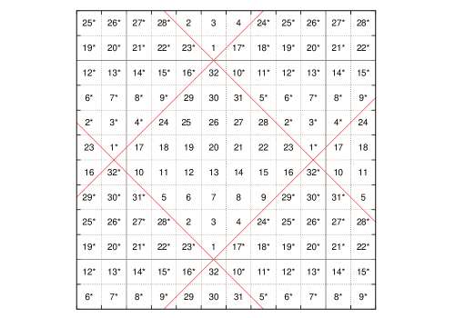
Figure 11: Shown is an $8\times 8$ square lattice of iron atoms under periodic boundary conditions that is split into two tilted squares. (See ref. [46].) The unique site that is farthest away from site $i$ is labeled by $i^{*}$.

It is instructive to compute the above Gutzwiller wavefunction in the case where the Fermi level $\varepsilon_{+}$ lies above the maximum of both bands at ${\bi k}=0$. The Fermi gas (3desacajbe) is then a Slater determinant over all of the allowed one-electron states restricted to “black squares” of the “checkerboard” in 2D momentum. It is evaluated directly in Appendix B, Eq. (LABEL:slater_deter_intrmdt). The Gutzwiller projection of it (3desacajbh) is a product of spin-singlet pairs within the $d+$ and $d-$ orbitals that entangle opposite spins separated by the maximum displacement ${\bi L}_{*}$:

$$\langle 1,\ldots,{\cal N}|\Psi_{0}\rangle={1\over{\sqrt{2^{N_{\rm Fe}}{\cal N}!}}}\sum_{p}({\rm sgn}\,p)\prod_{m=1}^{N_{\rm Fe}} {1\over\sqrt{2}}(\uparrow_{p(m)}\downarrow_{p(m^{\prime})}-\downarrow_{p(m)}\uparrow_{p(m^{\prime})})\cdot$$

$$\cdot\langle p(m),p(m^{\prime})|\alpha_{m},i_{m};\alpha_{m},i_{m}^{*}\rangle_{+},$$

where $m^{\prime}=m+N_{\rm Fe}$, and where $|\alpha,i;\beta,j\rangle_{+}=(|\alpha,i\rangle|\beta,j\rangle+|\beta,j\rangle|\alpha,i\rangle)/\sqrt{2}$. Here $(\alpha_{1},i_{1}),(\alpha_{2},i_{2}),\ldots,(\alpha_{N_{\rm Fe}},i_{N_{\rm Fe}})$ is a list of all orbitals and of all sites within a single subsquare in Fig. 11. Above, $|\Psi_{0}\rangle$ describes a featureless paramagnetic insulator in a spin-singlet state: $\langle{\bi S}_{i,\alpha}\cdot{\bi S}_{j,\beta}\rangle=0$ for $j\neq i,i^{*}$ or for $\beta\neq\alpha$, and $({\bi S}_{i,\alpha}+{\bi S}_{i^{*},\alpha})|\Psi_{0}\rangle=0$. The former yields an average number of triplets per iron site of $\langle({\bi S}_{i,d+}+{\bi S}_{i,d-})^{2}\rangle/2\hbar^{2}=3/4$. It lies halfway in between the value of $1/2$ for the naive hidden ferromagnetic state with perfect $\nwarrow_{d+}\searrow_{d-}$ spin order and the maximum value of $1$ when Hund’s Rule is obeyed. The value $3/4$ also coincides with the probability that a given iron atom be found in a spin-$1$ state. It must also be mentioned that the featureless paramagnetic insulator (LABEL:slater_deter_half_fill) is translationally invariant and $4$-fold rotationally invariant.

The paramagnetic nature of the Gutzwiller wave function (3desacajbh) at half filling (LABEL:slater_deter_half_fill) suggests that it describes a normal metallic phase when the Fermi level $\varepsilon_{+}$ falls below the band maxima at zero 2D momentum in the Fermi gas state (3desacajbe). Evaluating it becomes non-trivial then, however. We can get some idea of the nature of long-wavelength spin correlations in the Gutzwiller wave function (3desacajbh) away from half filling by artificially turning off all of the interactions in the two-orbital $t$-$J$ model (LABEL:tJ). This leaves us with the Fermi gas state (3desacajbe) and with the hopping terms in the Hamiltonian. It results in two hole Fermi surface pockets centered at zero 2D momentum, which are depicted by Fig. 2. We can then compute the dynamical auto-correlation of the true spin ($+$) and of the hidden spin ($-$) at the longwavelength limit, $N_{\rm Fe}^{-1/2}\sum_{i}({\bi S}_{i,d-}\pm{\bi S}_{i,d+})$, within this approximation. Explicit Lindhard functions for the dynamical spin-spin auto-correlation function in multi-orbital Fermi gases are given in ref. [8]. Substituting the matrix elements for the one-electron states (3desacajbg) into those expressions yields the following results at the long wavelength limit: $\langle{\bi S}(+)\cdot{\bi S}^{\prime}(+)\rangle|_{0,\omega}=0$ and

$$i\langle{\bi S}(-)\cdot{\bi S}^{\prime}(-)\rangle|_{0,\omega}^{\perp}={\hbar^{2}\over{N_{\rm Fe}}}\sum_{k_{0}}\sum_{\bi k}^{\qquad\prime}{n_{F}(k_{0},{\bi k})-n_{F}(k_{0}+\pi,{\bi k})\over{\omega+\varepsilon_{e}(k_{0}+\pi,{\bi k})-\varepsilon_{e}(k_{0},{\bi k})+i0^{+}}}.$$ (3desacajbj)

Above, the symbol $\perp$ indicates that the dot product is restricted to the $x$ and $y$ components of the spin, the prime notation indicates that the summation over 2D momentum is restricted to the “black squares” of the “checkerboard”, and $n_{F}(k)=\theta[\varepsilon_{+}-\varepsilon_{e}(k)]$ at zero temperature. True spin fluctuations at ${\bi q}=0$ are therefore absent. On the other hand, at zero temperature and $\omega>0$, the imaginary part of the above expression for hidden spin fluctuations at ${\bi q}=0$ reduces to

$${\rm Re}\,\langle{\bi S}(-)\cdot{\bi S}^{\prime}(-)\rangle|_{0,\omega}^{\perp}={\pi\hbar^{2}\over{N_{\rm Fe}}}\sum_{\bi k}^{\qquad\prime}n_{F}(0,{\bi k})[1-n_{F}(\pi,{\bi k})]\delta[\omega-2|\varepsilon_{\perp}({\bi k})|].$$ (3desacajbk)

The particle-hole occupation factors in the sum above restrict momenta to lie in between the two hole-pocket Fermi surfaces that are shown in Fig. 2. The present approximation therefore predicts hidden spin fluctuations at long wavelength, at frequencies inside of the range $[\omega_{1},\omega_{2}]$, with $\omega_{1}=2\,{\rm min}\,|\varepsilon_{\perp}|$ and $\omega_{2}=2\,{\rm max}\,|\varepsilon_{\perp}|$ for momenta restricted to lie in between the two hole pockets. At low hole concentration, $x_{+}\ll 1$, and at low inter-orbital hopping, $|t_{\perp}|,|t_{\perp}^{\prime}|\ll-t_{\parallel}$, Eqs. (3desacajak) and (3desacajal) for the hole-pocket Fermi surfaces yield that the limits in frequency are approximately $\omega_{1}\cong 8\pi x_{+}\,{\rm min}\,([1-|t_{\perp}|/(-t_{\parallel})]|t_{\perp}|,[1-|t_{\perp}^{\prime}|/(-t_{\parallel})]|t_{\perp}^{\prime}|)$ and $\omega_{2}\cong 8\pi x_{+}\,{\rm max}\,([1+|t_{\perp}|/(-t_{\parallel})]|t_{\perp}|,[1+|t_{\perp}^{\prime}|/(-t_{\parallel})]|t_{\perp}^{\prime}|)$. Expression (3desacajbk) also yields that the integrated spectral weight of the hidden spin fluctuations, $A(-,0)=\int_{0}^{\infty}d\omega\,{\rm Re}\,\langle{\bi S}(-)\cdot{\bi S}^{\prime}(-)\rangle|_{0,\omega}^{\perp}$, is proportional to the fraction of momentum space that lies in between the two hole pockets shown in Fig. 2: $A(-,0)=(\pi\hbar^{2}/N_{\rm Fe})\sum_{\bi k}^{\prime}n_{F}(0,{\bi k})[1-n_{F}(\pi,{\bi k})]$. It is of order $A(-,0)/\hbar^{2}\sim x_{+}\,{\rm max}(|t_{\perp}|,|t_{\perp}^{\prime}|)/(-t_{\parallel})$ within the present limits. This estimate for the spectral weight of hidden spin fluctuations at the long wavelength limit must be compared to the divergent spectral weight (3desacajbb) predicted by mean-field theory for the hidden half-metal state. The range of hidden magnetic correlations is finite in the former case, whereas it is infinite in the latter case.

Recall the exact energy spectrum of one hole in the $t$-$J$ model (LABEL:tJ) displayed by Fig. 5, at Hund’s Rule coupling of moderate strength, and in the absence of inter-orbital next-nearest-neighbor hopping, $t_{2}^{\perp}=0$. Low-energy electronic states emerge at cSDW momenta with specific orbital character. It suggests the following modification to the Fermi-gas part (3desacajbe) of the variational state (3desacajbh) that adds emergent nesting of Fermi surfaces at cSDW momenta:

$$|\Phi_{0}(x_{+},x_{-})\rangle=\prod_{k_{0},{\bi k},s}^{\qquad\prime}c_{s}(\pi,{\bi k+{\bi Q_{k}}})^{\dagger}|\Phi_{0}(x_{+},0)\rangle\quad{\rm with}\quad\varepsilon_{e}(k_{0},{\bi k})>\varepsilon_{-},$$ (3desacajbl)

where ${\bi Q}_{k_{0},{\bi k}}=(\pi/a){\hat{\bi x}}$ if $P_{\bi Q}(k_{0},{\bi k};\pi,{\bi k}+{\bi Q})>1/2$, and where ${\bi Q}_{k_{0},{\bi k}}=(\pi/a){\hat{\bi y}}$ if $P_{\bi Q}(k_{0},{\bi k};\pi,{\bi k}+{\bi Q})>1/2$. Here, $P_{\bi Q}(k;k^{\prime})=|\sum_{\alpha}\sum_{i}\phi_{k}^{*}(\alpha,i)e^{-i{\bi Q}\cdot{\bi r}_{i}}\phi_{k^{\prime}}(\alpha,i)|^{2}$ is the nesting probability between two eigenstates of the hopping Hamiltonian for free electrons. Substituting in the form (3desacajbg) for the eigenstates yields $P_{\bi Q}(\pi,{\bi k};\pi,{\bi k}+{\bi Q})={\rm cos}^{2}[\delta_{e}({\bi k})-\delta_{e}({\bi k}+{\bi Q})]$ and $P_{\bi Q}(0,{\bi k};\pi,{\bi k}+{\bi Q})={\rm sin}^{2}[\delta_{e}({\bi k})-\delta_{e}({\bi k}+{\bi Q})]$. The above variational state (3desacajbl) requires unoccupied one-electron states that carry nested $3$-momenta $(\pi,{\bi k}+{\bi Q}_{k_{0},{\bi k}})$ in the Fermi gas $\Phi_{0}(x_{+},0)$ (3desacajbe). Hence, $N/2$ must be odd. The nested Fermi surfaces of the Fermi gas (3desacajbl) are displayed by Fig. 8 for negative $t_{1}^{\perp}(\hat{\bi x})=-t_{1}^{\perp}(\hat{\bi y})$ and $t_{2}^{\perp}=0$. In the general case with hybridization, where $t_{2}^{\perp}(\hat{\bi x}+\hat{\bi y})=-t_{2}^{\perp}(-\hat{\bi x}+\hat{\bi y})$ is pure imaginary, Eq. (3desacag) for the inter-orbital hopping matrix element yields that $\delta_{e}({\bi k})\cong 0$ for ${\bi k}$ near $(\pi/a)\hat{\bi x}$ and that $\delta_{e}({\bi k})\cong\pi/2$ for ${\bi k}$ near $(\pi/a)\hat{\bi y}$. Also, $\delta_{e}({\bi k})$ winds around the hole pockets following (3desacajan) for ${\bi k}$ near zero 2D momentum. In the general case, the pattern of nesting defined above is then simply that described by Fig. 8, but with hybridization between the $3d_{xz}$ and $3d_{yz}$ orbitals included.

At perfect nesting, $\varepsilon_{+}=\varepsilon_{-}$, the Gutzwiller projection (3desacajbh) of the Slater determinant (3desacajbl) is necessarily a Mott insulator at half filling: $x_{+}=x_{-}$. It is therefore a variational groundstate for the corresponding two-orbital Heisenberg model over the square lattice. Both exact and spin-wave analyses of that model finds evidence for a quantum-critical transition between a hidden ferromagnetic state at weak Hund coupling and a cSDW at strong Hund coupling[14]. (See Fig. 1.) The perfect nesting of the Fermi gas (3desacajbl) at half filling suggests, however, that its Gutzwiller projection $\Psi_{0}$ shows strict long-range cSDW order. We therefore conjecture that the Gutzwiller projection (3desacajbh) of (3desacajbl) at half filling is a weak cSDW. Excluding possible renormalizations, it has a spin stiffness[47] $\rho_{s}=S_{*}^{2}J_{1}$, with an ordered moment $S_{*}\sim x_{+}^{1/2}$. Notice that such stripe spin order is consistent with the product of spin-singlet pairs (LABEL:slater_deter_half_fill) at the limit $x_{\pm}\rightarrow 0$ only if $N/2$ is odd, as required, in which case the pairs of opposing spins are separated by the maximum displacement ${\bi L}_{*}=(N/2)a(\hat{\bi x}\pm\hat{\bi y})$. Two metallic cases exist off half filling. The hole Fermi surfaces centered at zero 2D momentum are larger than the nested ones centered at cSDW momenta for $\varepsilon_{+}<\varepsilon_{-}$, where the net concentration of mobile holes at site-orbitals is proportional to the difference in area between the two: $x=x_{+}-x_{-}$. The Gutzwiller projection (3desacajbh) then yields a variational wavefunction for the $t$-$J$ model (LABEL:tJ) that lies below half filling in this case. At $\varepsilon_{+}>\varepsilon_{-}$, on the other hand, the area of the Fermi surfaces centered at cSDW momenta is larger, and the Gutzwiller projection (3desacajbh) now has a net concentration of electrons at site-orbitals instead of holes: $-x=x_{-}-x_{+}$. Each mobile electron must form a spin singlet with a local moment at the site-orbital in the present infinite-$U_{0}$ limit.

We now argue for electron-type dispersion of the low-energy electronic structure that emerges at cSDW momenta for Hund’s Rule coupling of moderate strength in the two-orbital $t$-$J$ model (LABEL:tJ) with off-diagonal magnetic frustration. Let us confine ourselves to the ideal case $t_{2}^{\perp}=0$ shown by Fig. 5. The $3d_{xz}$ and $3d_{yz}$ orbitals are then good quantum numbers, which we now label by $k_{0}=0$ and $\pi$, respectively. The phase factors in the one-electron states (3desacajbg) can then be set to unity ($\delta_{e}=0$), which means that the one-hole energy (3desaa) instead becomes $-\varepsilon_{e}(k_{0},{\bi k})=\varepsilon_{\parallel}({\bi k})+e^{ik_{0}}\varepsilon_{\perp}({\bi k})$. Above, the nesting wave vectors for the $3d_{xz}$ and $3d_{yz}$ orbitals are respectively ${\bi Q}_{0}=(\pi/a){\hat{\bi y}}$ and ${\bi Q}_{\pi}=(\pi/a){\hat{\bi x}}$. Assume that the low-energy electronic structure displayed by Fig. 5 is described by a renormalized energy band $\tilde{\varepsilon}_{e}(k_{0},{\bi k})$ that remains hole-type near ${\bi k}=0$. In the present case, where the $3d_{xz}$ and $3d_{yz}$ orbitals are good quantum numbers, the dynamical correlation function for true spin fluctuations at cSDW momenta reduces to the standard Lindhard function (see ref. [8]):

$${\rm Re}\,\langle{\bi S}(+)\cdot{\bi S}^{\prime}(+)\rangle|_{{\bi Q}_{k_{0}},\omega}^{\perp}\cong{\pi\hbar^{2}\over{N_{\rm Fe}}}\sum_{\bi k}^{\qquad\prime} n_{F}(k_{0},{\bi k})[1-n_{F}(k_{0},{\bi k}+{\bi Q}_{k_{0}})]\cdot$$

$$\cdot(\delta[\omega-\tilde{\varepsilon}_{e}(k_{0},{\bi k}+{\bi Q}_{k_{0}})+\tilde{\varepsilon}_{e}(k_{0},{\bi k})]$$

$$-\delta[\omega+\tilde{\varepsilon}_{e}(k_{0},{\bi k}+{\bi Q}_{k_{0}})-\tilde{\varepsilon}_{e}(k_{0},{\bi k})]).$$

Here, we have used the fact that ${\bi Q}_{k_{0}}+{\bi Q}_{k_{0}}=0$. Importantly, expression (LABEL:true_spin_fluct) predicts that low-energy cSDW spin fluctuations exist when the renormalized band $\tilde{\varepsilon}_{e}(k_{0},{\bi k})$ crosses the Fermi level both near ${\bi k}=0$ and near ${\bi k}={\bi Q}_{k_{0}}$. Assume next an electron-type dispersion for the nested band of emergent one-particle states. The spectral weight for such spin fluctuations, $A(+,{\bi Q}_{k_{0}})=\int_{0}^{\infty}d\omega\,{\rm Re}\,\langle{\bi S}(+)\cdot{\bi S}^{\prime}(+)\rangle|_{{\bi Q}_{k_{0}},\omega}^{\perp}$, is then of order $\pi\hbar^{2}$ because of the particle-hole factors in expression (LABEL:true_spin_fluct). This result is consistent with the present local-moment description (LABEL:tJ) of a cSDW metal with short-range antiferromagnetic order. On the other hand, like hidden spin fluctuations (3desacajbk), a hole-type dispersion for the emergent band results in a relatively small spectral weight that instead is equal to $\pi\hbar^{2}|x_{+}-x_{-}|$, where $x_{+}$ and $x_{-}$ are the concentrations of holes within the Fermi surface pockets centered at zero 2D momentum and centered at cSDW momenta, respectively. It vanishes at half filling, $x_{+}=x_{-}$, which implies that no cSDW spin fluctuations exist in such case. In particular, no spin fluctuations at cSDW momenta should exist at the quantum-critical point that separates hidden magnetic order at weak Hund coupling from cSDW order at strong Hund coupling in the corresponding frustrated two-orbital Heisenberg model over the square lattice[14]. Also, no long-range magnetic order of either type exists at the quantum-critical point. Application of the quantum-fluids analogy for frustrated antiferromagnets[47] at a quantum critical point then yields that there exist absolutely no low-energy spin excitations that carry cSDW momenta there, neither “superfluid” nor “normal”. We believe that this is unlikely. A comparison of the spectral weights for cSDW spin fluctuations therefore argues in favor of electron-type dispersion for the nested band of one-particle states that emerges at cSDW momenta.

In conclusion, we propose a cSDW metal groundstate, Eqs. (3desacajbe), (3desacajbh) and (3desacajbl), for the two-orbital $t$-$J$ model with off-diagonal frustration, at moderate Hund’s Rule coupling. It is suggested both by Schwinger-boson-slave-fermion mean-field theory and by exact results for the low-energy spectrum of one mobile hole. It notably shows low-energy hidden spin fluctuations at the long-wavelength limit because of nesting between the two hole-pockets centered at zero 2D momentum. (See Fig. 2.) This type of hidden spin fluctuation may play an important role in the formation of Cooper pairs in iron-pnictide materials. Last, the same arguments can be applied to the hole-pocket Fermi surfaces obtained from DFT[6][7][8], which are similar to those depicted by Fig. 2. In particular, the application of expression (3desacajbj) implies that low-energy hidden spin fluctuations must also exist at the long wavelength limit in such case.

6 Discussion and Conclusions

Starting from a local-moment description of a cSDW over a square lattice of spin-$1$ iron atoms with mobile holes, we have succeeded in accounting for the nested Fermi surface pockets centered at zero 2D momentum and at cSDW momenta that are characteristic of iron-pnictide high-temperature superconductors. In particular, zero-energy spin-wave excitations at cSDW momenta combine with hole Fermi surface pockets centered at zero 2D momentum to produce Fermi surface pockets centered at cSDW momenta. The former hole pockets exist because of proximity to a hidden half metal state with opposing polarized spin over $3d_{(x+iy)z}$ and $3d_{(x-iy)z}$ orbitals, respectively, which violates Hund’s Rule. The isotropic $(d+,d-)$ orbital basis that we choose notably maximizes the Hund’s Rule coupling (see Appendix A), and it leads to isotropic Heisenberg exchange coupling constants across neighboring spins on the square lattice of iron atoms. This orbital basis then very likely minimizes the net magnetic energy in the two-orbital $t$-$J$ model (LABEL:tJ) at fixed iron moment, $\langle|\sum_{\alpha}{\bi S}_{i,\alpha}|^{2}\rangle^{1/2}$. Notice that the emergent Fermi-surface nesting uncovered here is a mirror image of weak-interaction descriptions for electronic structure in iron-pnictide high-temperature superconductors, where low-energy spin excitations centered at cSDW momenta are a result of Fermi surface nesting[6][7][8]. The present local-moment description has also revealed the existence of hidden low-energy spin excitations between the $d+$ and $d-$ orbitals that is intimately tied to nesting between the two hole pockets centered at zero 2D momentum. DFT calculations of the electronic structure in iron-pnictide materials[6][7][8] also exhibit concentric hole-pocket Fermi surfaces similar to those depicted by Fig. 2. We therefore suggest that hidden low-energy spin-fluctuations at the long wavelength limit are predicted by DFT as well.

It is useful to contrast our results with those of more ad hoc theoretical models that separate local moments from itinerant electrons[48][49]. Although such models are capable of simultaneously accounting for the spin-wave spectra and for the Fermi surfaces seen in iron-pnictide high-temperature superconductors and their parent compounds, they clearly have less predictive power by virtue of the explicit separation between the two phenomena. Early models for iron-pnictide systems that simply add Heisenberg exchange interactions and Hund coupling to one-electron hopping Hamiltonians that already include nested Fermi surfaces, but that do not project out double occupancy at an iron site-orbital, also suffer from this drawback in our opinion[50]. In particular, such models essentially operate in the weak-interaction limit, but they fail to link Fermi surface nesting to low-energy spin excitations at cSDW momenta in iron-pnictide high-temperature superconductors.

In summary, a mean-field theory analysis and an exact diagonalization study indicate that the two-orbital $t$-$J$ model (LABEL:tJ) for iron-pnictide high-temperature superconductors transits from a cSDW to a hidden half-metal state with decreasing Hund’s Rule coupling if off-diagonal magnetic frustration exists: $J_{1}^{d\pm,d\pm}<J_{1}^{d\pm,d\mp}$, $J_{1}^{d\pm,d\mp}>0$ and $J_{2}^{\alpha,\beta}>0$. Equation (3desacajav) for the critical Hund coupling implies that moving off the QCP by a few percent in the hole concentration leads to a relatively small deviation: $|\delta J_{0c}/J_{0c}|\cong 4|t_{\parallel}\delta x/J_{0c}|$. We propose that the quantum critical point predicted by the mean-field theory and by exact results (Fig. 5) controls the phase diagram of iron-pnictide high-$T_{c}$ superconductors in the vicinity of the transition to the cSDW. This proposal is consistent with the low-energy spin-excitation spectrum and with the low-energy electronic structure shown by these systems. In particular, Schwinger-boson-slave-fermion mean-field theory (3desacajba) predicts low-energy spinwaves that disperse anisotropically at cSDW momenta, $(\pi/a){\hat{\bi x}}$ and $(\pi/a){\hat{\bi y}}$, near the quantum critical point that separates the hidden half metal from the cSDW. The predicted dispersion of the spinwave spectrum, Fig. 3, notably shows a local maximum at the Néel wavenumber $(\pi/a)({\hat{\bi x}}+{\hat{\bi y}})$, which agrees with inelastic neutron scattering studies of the parent compound CaFe₂As₂ [15]. Further, the anisotropic dispersion that we predict at the QCP for low-energy spinwaves with cSDW momenta is consistent with recent observations of the same in iron-pnictide superconductors[17][18][19][20]. And in agreement with what ARPES reveals for the electronic structure in iron-pnictide systems[2][3][4][5], both the Schwinger-boson-slave-fermion mean-field theory formulation (3desacajbc) and exact diagonalization of the two-orbital $t$-$J$ model (LABEL:tJ) predict nested Fermi surface pockets around zero 2D momentum and around cSDW momenta with purely $3d_{xz}$ and $3d_{yz}$ orbital character at the quantum critical point. The dispersion of the former is hole type by construction, whereas arguments put forth at the end of the previous section indicate that the dispersion of the latter is electron type. Recent ARPES on optimally doped Ba(Fe_1-xCo_x)₂As₂ notably find similar electron-pocket Fermi surfaces around cSDW momenta with purely $3d_{xz}$ and $3d_{yz}$ orbital character[5].

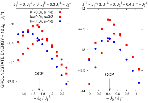
Figure 12: How groundstate degeneracy breaks as the Hund’s Rule coupling moves off the QCP is displayed for one hole that roams over a $4\times 4\times 2$ lattice in the two-orbital $t$-$J$ model. Hopping matrix elements are set to $t_{1}^{\parallel}=-5(J_{1}^{\parallel}+J_{1}^{\perp})$, $t_{1}^{\perp}({\hat{\bi x}})=-2(J_{1}^{\parallel}+J_{1}^{\perp})$, $t_{1}^{\perp}({\hat{\bi y}})=+2(J_{1}^{\parallel}+J_{1}^{\perp})$, and $t_{2}^{\parallel}=0=t_{2}^{\perp}$.

We finish by pointing out that more recent experimental determinations of the electronic structure in interfacial iron selenides find evidence for superconductivity with a record critical temperature[23][24]. In particular, ARPES on a single layer of FeSe sees an isotropic superconducting gap at the electron Fermi surface pockets centered at cSDW momenta that closes at $T_{c}=65$-$70$ K [25][26]. Importantly, ARPES also reveals that the hole bands centered at zero 2D momentum lie below the Fermi level in general. This experimental observation conflicts with DFT calculations on interfacial iron selenides, which predict that such hole bands should cross the Fermi surface[27]. We suggest, instead, that interfacial high-$T_{c}$ superconductivity in iron selenides is consistent with the quantum critical point found here. Figure 12 plots the evolution of the lowest energy levels near the QCP as a function of Hund’s Rule coupling strength. The energies are exact values for the two-orbital $t$-$J$ model (LABEL:tJ) over a $4\times 4\times 2$ lattice with one mobile hole. Next-nearest neighbor hopping is turned off, which yields exact particle-hole symmetry. Figure 12 therefore also accurately describes the evolution of the corresponding groundstate energies for one mobile electron above half filling. Notice that the groundstate at momentum $(\pi/a)\hat{\bi x}$ lies below the groundstate at zero momentum for Hund’s Rule coupling that is stronger than the critical value. The maximum energy difference between those two states in the left panel is approximately $\Delta\varepsilon_{e,h}=J_{1}^{\perp}/3$ at $J_{0}=-1.95\,J_{1}^{\perp}$. It is a good fraction of the maximum dispersion of the low-energy spin-$1/2$ states shown in Fig. 5. ARPES on mono-layer FeSe superconductors find a difference in energy of $\Delta\varepsilon_{e,h}=15$ meV between the bottom of the electron band and the top of the hole band[25]. Comparing these two yields a lower bound for the Heisenberg exchange coupling constant of order $J_{1}^{\perp}\gtrsim 50$ meV. Fits of the spin-wave spectrum predicted by the corresponding two-orbital Heisenberg model to the dispersion of the spin resonance in Ba(Fe_1-xCo_x)₂As₂ [17] yield a value of $J_{1}^{\perp}\gtrsim 100$ meV[14], which lies inside this range. Last, the right panel in Fig. 12 demonstrates that the emergent electronic structure at cSDW momenta is robust in the presence of intra-orbital Heisenberg exchange $J_{1}^{\parallel}>0$. The evolution of the groundstate energy levels with Hund’s Rule coupling described above therefore potentially accounts for the absence of hole-pocket Fermi surfaces at zero 2D momentum in single-layer FeSe.

Appendix A

Here we calculate the Hund’s Rule coupling in the 2D subspace spanned by the $3d_{xz}$ and $3d_{yz}$ orbitals in iron-pnictide materials. Consider the most general pair of basis states for such orbitals:

$$\phi({\bi r}) =R_{3,2}(r)[(\cos\alpha_{0})e^{-i\phi_{0}}Y_{2,+1}(\Omega)+(\sin\alpha_{0})e^{+i\phi_{0}}Y_{2,-1}(\Omega)],$$ (3desacajbna)

$$\psi({\bi r}) =R_{3,2}(r)[-(\sin\alpha_{0})e^{-i\phi_{0}}Y_{2,+1}(\Omega)+(\cos\alpha_{0})e^{+i\phi_{0}}Y_{2,-1}(\Omega)].$$ (3desacajbnb)

Notice that $\alpha_{0}=0$ or $\pi/2$ corresponds to the $3d_{(x+iy)z}$/$3d_{(x-iy)z}$ orbital basis, whereas $\alpha_{0}=\pi/4$ and $\phi_{0}=0$ corresponds to the $3d_{xz}$/$3d_{yz}$ orbital basis. The exchange Coulomb integral is related to the Hund’s Rule exchange coupling constant $J_{0}$ by

$$-{1\over 2}J_{0}=\int d^{3}r_{1}\int d^{3}r_{2}\,\phi^{*}({\bi r_{1}})\psi({\bi r_{1}}){e^{2}\over{|{\bi r_{1}}-{\bi r_{2}}|}}\psi^{*}({\bi r_{2}})\phi({\bi r_{2}})$$ (3desacajbnbo)

in general. In the present case, this yields

$$-{1\over 2}J_{0}=\int d^{3}r_{1} \int d^{3}r_{2}\,R_{3,2}^{2}(r_{1})[(\cos\alpha_{0})^{2}Y_{2,+1}^{2}(\Omega_{1}^{\prime})-(\sin\alpha_{0})^{2}Y_{2,-1}^{2}(\Omega_{1}^{\prime})]$$

$$\cdot{e^{2}\over{|{\bi r_{1}}-{\bi r_{2}}|}}R_{3,2}^{2}(r_{2})[(\cos\alpha_{0})^{2}Y_{2,+1}^{*2}(\Omega_{2}^{\prime})-(\sin\alpha_{0})^{2}Y_{2,-1}^{*2}(\Omega_{2}^{\prime})],$$

where $\Omega^{\prime}$ is the solid angle rotated by $\phi_{0}$ about the $z$ axis. The integrals over solid angles $\Omega_{1}^{\prime}$ and $\Omega_{2}^{\prime}$ can be performed in the standard way[51] by use of the mathematical identity

$${1\over{|{\bi r_{1}}-{\bi r_{2}}|}}=\sum_{l=0}^{\infty}{r_{<}^{l}\over{r_{>}^{l+1}}}{4\pi\over{2l+1}}\sum_{m=-l}^{l}Y_{l,m}(\Omega_{1}^{\prime})Y_{l,m}^{*}(\Omega_{2}^{\prime})$$ (3desacajbnbp)

combined with addition of angular momentum:

$$Y_{2,\pm 1}^{2}(\Omega)={1\over 7}\Biggl{(}{15\over{2\pi}}\Biggr{)}^{1/2}Y_{2,\pm 2}(\Omega)+{1\over 7}\Biggl{(}{10\over{\pi}}\Biggr{)}^{1/2}Y_{4,\pm 2}(\Omega).$$ (3desacajbnbq)

Performing the remaining radial integrals after substitution of the hydrogenic radial wave function

$$R_{3,2}(r)={2\over{81}}\Biggl{(}{2\over{15a_{0}^{3}}}\Biggr{)}^{1/2}\Biggl{(}{r\over{a_{0}}}\Biggr{)}^{2}e^{-r/3a_{0}}$$ (3desacajbnbr)

then yields the final result

$$-{1\over 2}J_{0}={1\over{(2\cdot 3)^{5}(5\cdot 7)^{2}}}\Biggl{[}3\,I_{2}+5\Biggl{(}{2\over 3}\Biggr{)}^{2}I_{4}\Biggr{]}{e^{2}\over{a_{0}}}(\cos^{4}\alpha_{0}+\sin^{4}\alpha_{0}),$$ (3desacajbnbs)

where

$$I_{4}={12!\over{2^{12}}}\Biggl{(}{2\over 11}-{1\over 12}\Biggl{)}$$ (3desacajbnbt)

and

$$I_{2}={12!\over{2^{12}}}\Biggl{(}{2^{3}\over 9}-3{2^{2}\over 10}+3{2\over 11}-{1\over 12}\Biggl{)}$$ (3desacajbnbu)

are the strengths of the integrals due to the $l=4$ and $l=2$ channels, respectively. Note that the binomial-like series that appear above result from the difference

$$(5-l)!-2^{-(6-l)}s_{11}^{(5-l)}(1/2),$$

where $s_{n}^{(m)}(x)$ is the $m^{\rm th}$ derivative of the finite geometric series sum $s_{n}(x)=\sum_{k=0}^{n}x^{k}$. The Hund’s Rule coupling is then

$$-J_{0}={1\over 30.3082}\,{e^{2}\over 2a_{0}}(\cos^{4}\alpha_{0}+\sin^{4}\alpha_{0}).$$ (3desacajbnbv)

Notice that $\cos^{4}\alpha_{0}+\sin^{4}\alpha_{0}=1-{1\over 2}\sin^{2}2\alpha_{0}$, which reaches its maximum value of unity at $\alpha_{0}=0$ or $\pi/2$ and its minimum value of $1/2$ at $\alpha_{0}=\pi/4$. We conclude that the Hund’s Rule coupling is largest in the isotropic $3d_{(x+iy)z}$/$3d_{(x-iy)z}$ orbital basis, while it is smallest in the anisotropic $3d_{xz}$/$3d_{yz}$ orbital basis from Chemistry.

It is useful to compare the maximum Hund’s Rule coupling in the isotropic $3d_{(x+iy)z}$/$3d_{(x-iy)z}$ orbital basis with the on-site Coulomb repulsion in that case:

$$U_{0}=\int d^{3}r_{1}\int d^{3}r_{2}\,R_{3,2}^{2}(r_{1})|Y_{2,1}(\Omega_{1})|^{2}{e^{2}\over{|{\bi r_{1}}-{\bi r_{2}}|}}R_{3,2}^{2}(r_{2})|Y_{2,1}(\Omega_{2})|^{2}.$$ (3desacajbnbw)

Addition of angular momentum yields the identity

$$|Y_{2,1}(\Omega)|^{2}={1\over{7\pi}}P_{0}(\cos\theta)+{5\over{28\pi}}P_{2}(\cos\theta)-{3\over{7\pi}}P_{4}(\cos\theta)$$ (3desacajbnbx)

in terms of Legendre polynomials. Substituting it above, with $P_{l}(\cos\theta)=[4\pi/(2l+1)]^{1/2}Y_{l,0}(\Omega)$, along with the mathematical identity (3desacajbnbp), yields the result

$$U_{0}={1\over{2^{6}3^{5}5^{2}}}\Biggl{[}I_{0}+{1\over{7^{2}}}I_{2}+\Biggl{(}{4\over{3\cdot 7}}\Biggl{)}^{2}I_{4}\Biggr{]}{e^{2}\over{a_{0}}}$$ (3desacajbnby)

for the Coulomb integral, where

$$I_{0}={12!\over{2^{12}}}\Biggl{(}{2^{5}\over 7}-5{2^{4}\over 8}+10{2^{3}\over 9}-10{2^{2}\over 10}+5{2\over 11}-{1\over 12}\Biggl{)}$$ (3desacajbnbz)

is the strength of the integral in the $l=0$ channel. The ratio of the on-site Coulomb repulsion (3desacajbnby) to the Hund’s Rule coupling (3desacajbnbs) is then

$$-{2U_{0}\over{J_{0}}}=10.6743.$$ (3desacajbnca)

Study of the exchange integral (3desacajbnbo) yields that this ratio coincides with the ratio $J_{1}^{d+,d+}({\rm drct})/J_{1}^{d+,d-}({\rm drct})$ in the regime $a_{0}\gg a$.

Appendix B

Here, we evaluate the Gutzwiller projection (3desacajbh) of the “filled” Fermi gas (3desacajbe). Specifically, the Fermi level $\varepsilon_{+}$ (and $\varepsilon_{-}$) lies above the maximum of both bands, $\varepsilon_{e}(0,{\bi k})$ and $\varepsilon_{e}(\pi,{\bi k})$, at ${\bi k}=0$. The Fermi gas (3desacajbe) is then a Slater determinant over all of the allowed one-electron states restricted to “black squares” of the “checkerboard” in 2D momentum. It can be written in the form

$$\Phi_{0}(1,\ldots,{\cal N})=({\cal N}!)^{-1/2}\sum_{[q]}\sum_{p\in[q]}({\rm sgn}\,p) \Biggl{[}\prod_{m=1}^{N_{\rm Fe}}\phi_{k_{m}}(p(m))\uparrow_{p(m)}\Biggr{]}\cdot$$

$$\cdot\Biggl{[}\prod_{n=1+N_{\rm Fe}}^{\cal N}\phi_{k_{n^{\prime}}}(p(n))\downarrow_{p(n)}\Biggr{]},$$

where $n^{\prime}=n-N_{\rm Fe}$, and where $[q]$ denote equivalence classes of permutations $p$ that do not flip any spins. In particular, we can write $p=qp_{\uparrow}p_{\downarrow}$, where $p_{\uparrow}$ and $p_{\downarrow}$ denote permutations of $1,2,\ldots,N_{\rm Fe}$ and of $1+N_{\rm Fe},2+N_{\rm Fe},\ldots,{\cal N}$ respectively. Above, $k_{1},k_{2},\ldots,k_{N_{\rm Fe}}$ is a list of all 3-momenta on the “black squares”. The Slater determinant (LABEL:slater_deter) can then be written more explicitly as

$$\Phi_{0}(1,\ldots,{\cal N})=({\cal N}!)^{-1/2} \sum_{[q]}({\rm sgn}\,q)\cdot$$

$$\cdot\Biggl{[}\sum_{p_{\uparrow}}({\rm sgn}\,p_{\uparrow})\prod_{m=1}^{N_{\rm Fe}}\phi_{k_{m}}(qp_{\uparrow}(m))\uparrow_{qp_{\uparrow}(m)}\Biggr{]}\cdot$$

$$\cdot\Biggl{[}\sum_{p_{\downarrow}}({\rm sgn}\,p_{\downarrow})\prod_{n=1+N_{\rm Fe}}^{\cal N}\phi_{k_{n^{\prime}}}(qp_{\downarrow}(n))\downarrow_{qp_{\downarrow}(n)}\Biggr{]}.$$

Application of the mathematical identity ${\rm det}\,AB=({\rm det}\,A)({\rm det}\,B)$ yields ${\rm det}\,\phi_{k_{m}}(n)=e^{i\phi_{0}}{\rm det}\,\delta_{\alpha_{m},\beta_{n}}(\delta_{i_{m},j_{n}}+\delta_{i_{m}^{*},j_{n}})/2^{1/2}$, where $e^{i\phi_{0}}={\rm det}\,2^{1/2}\phi_{k_{m}}(\alpha_{n},i_{n})$. Here $(\alpha_{1},i_{1}),(\alpha_{2},i_{2}),\ldots,(\alpha_{N_{\rm Fe}},i_{N_{\rm Fe}})$ is a list of all orbitals and of all sites within a single subsquare in Fig. 11. On the other hand, $\beta_{n}$ and $j_{n}$ represent the orbital and the site of electron $n$ with spin $\uparrow(\downarrow)$. The last determinant lies on the unit circle of the complex plane because its argument is an $N_{\rm Fe}\times N_{\rm Fe}$ unitary matrix. Substituting the previous identity in for the spin-up and for the spin-down determinants in expression (LABEL:slater_deter_explct) yields the following expression for the Slater determinant up to a phase factor:

$$\langle 1,\ldots,{\cal N}|\Phi_{0}\rangle= ({\cal N}!)^{-1/2}\sum_{p}({\rm sgn}\,p)\cdot$$

$$\cdot\Biggl{[}\prod_{m=1}^{N_{\rm Fe}}2^{-1/2}(\langle p(m)|\alpha_{m},i_{m}\rangle+\langle p(m)|\alpha_{m},i_{m}^{*}\rangle)\uparrow_{p(m)}\Biggr{]}\cdot$$

$$\cdot\Biggl{[}\prod_{n=1+N_{\rm Fe}}^{\cal N}2^{-1/2}(\langle p(n)|\alpha_{n^{\prime}},i_{n^{\prime}}\rangle+\langle p(n)|\alpha_{n^{\prime}},i_{n^{\prime}}^{*}\rangle)\downarrow_{p(n)}\Biggr{]}.$$

After grouping together common site-orbital factors into spin-singlet pairs, and subsequently projecting out double occupancy per site-orbital, we obtain the final expression for the Gutzwiller wavefunction:

$$\langle 1,\ldots,{\cal N}|\Psi_{0}\rangle={1\over{\sqrt{2^{N_{\rm Fe}}{\cal N}!}}}\sum_{p}({\rm sgn}\,p)\prod_{m=1}^{N_{\rm Fe}} {1\over\sqrt{2}}(\uparrow_{p(m)}\downarrow_{p(m^{\prime})}-\downarrow_{p(m)}\uparrow_{p(m^{\prime})})\cdot$$

$$\cdot\langle p(m),p(m^{\prime})|\alpha_{m},i_{m};\alpha_{m},i_{m}^{*}\rangle_{+},$$

where $m^{\prime}=m+N_{\rm Fe}$, and where $|\alpha,i;\beta,j\rangle_{+}=(|\alpha,i\rangle|\beta,j\rangle+|\beta,j\rangle|\alpha,i\rangle)/\sqrt{2}$. It describes a featureless paramagnetic insulator composed of a product of spin-singlet pairs within the same $d+$ and $d-$ orbitals that entangle opposite spins separated by the maximum displacement ${\bi L}_{*}$.

A hole excitation about the above spin-singlet paramagnetic insulator with 2D momentum on the “black squares” of the “checkerboard” is then just the Gutzwiller projection (3desacajbh) of the “filled” band (3desacajbe) with that state missing. To obtain a hole excitation that has momentum on the “white squares”, we repeat the previous calculation of the “filled” band case, but with the 2D momenta restricted to the “white squares”: ${\bi k}=(2\pi n_{x}/Na,2\pi n_{y}/Na)$, where $n_{x}$ and $n_{y}$ are respectively even and odd integers, or vice versa. The one-electron states are then antiperiodic on a tilted subsquare in Fig. 11. In particular, the relative plus sign between sites separated by the maximum displacement ${\bi L}_{*}$ in the one-electron states that appears in Eqs. (3desacajbg) and (LABEL:slater_deter_intrmdt) is replaced by a relative minus sign in this case. The Gutzwiller projection (LABEL:slater_deter_final) remains unchanged, however. A hole excitation with 2D momentum on the “white squares” then is simply the Gutzwiller projection (3desacajbh) of the “filled” band (3desacajbe) over the “white squares”, but with that state missing.

References

References

- [1] Y. Kamihara, T. Watanabe, M. Hirano, and H. Hosono, J. Am. Chem. Soc. 130, 3296 (2008).
- [2] V.B. Zabolotnyy, D.S. Inosov, D.V. Evtushinsky, A. Koitzch, A.A. Kordyuk, G.L. Sun, J.T. Park, D. Haug, V. Hinkov, A.V. Boris, C.T. Lin, M. Knupfer, A.N. Yaresko, B. Buchner, A. Varykhalov, R. Follath and S.V. Borisenko, Nature 457, 569 (2009).
- [3] J. Fink, S. Thirupathaiah, R. Ovsyannikov, H. A. Durr, R. Follath, Y. Huang, S. deJong, M. S. Golden, Yu-Zhong Zhang, H. O. Jeschke, R. Valenti, C. Felser, S. Dastjani Farahani, M. Rotter, and D. Johrendt, Phys. Rev. B 79, 155118 (2009).
- [4] V. Brouet, M. Marsi, B. Mansart, A. Nicolaou, A. Taleb-Ibrahimi, P. Le Fevre, F. Bertran, F. Rullier-Albenque, A. Forget, and D. Colson, Phys. Rev. B 80, 165115 (2009).
- [5] Y. Zhang, F. Chen, C. He, B. Zhou, B.P. Xie, C. Fang, W.F. Tsai, X.H. Chen, H. Hayashi, J. Jiang, H. Iwasawa, K. Shimada, H. Namatame, M. Taniguchi, J.P. Hu and D.L. Feng, Phys. Rev. B 83, 054510 (2011).
- [6] D.J. Singh and M.H. Du, Phys. Rev. Lett. 100, 237003 (2008).
- [7] J. Dong, H. J. Zhang, G. Xu, Z. Li, G. Li, W. Z. Hu, D. Wu, G. F. Chen, X. Dai, J. L. Luo, Z. Fang, N. L. Wang, Euro. Phys. Lett. 83, 27006 (2008).
- [8] S. Graser, T.A. Maier, P.J. Hirschfeld and D.J. Scalapino, New J. Phys. 11, 025016 (2009).
- [9] S. Raghu, Xiao-Liang Qi, Chao-Xing Liu, D. Scalapino, Shou-Cheng Zhang, Phys. Rev. B 77, 220503(R) (2008).
- [10] C. de la Cruz, Q. Huang, J.W. Lynn, J. Li, W. Ratcliff, J.L. Zarestky, H.A. Mook, G.F. Chen, J.L. Luo, N.L. Wang and P. Dai, Nature 453, 899 (2008).
- [11] Q. Si and E. Abrahams, Phys. Rev. Lett. 101, 076401 (2008).
- [12] J.P. Rodriguez and E.H. Rezayi, Phys. Rev. Lett. 103, 097204 (2009).
- [13] B. Schmidt, M. Siahatgar, P. Thalmeier, Phys. Rev. B 81, 165101 (2010).
- [14] J.P. Rodriguez, Phys. Rev. B 82, 014505 (2010).
- [15] Jun Zhao, D. T. Adroja, Dao-Xin Yao, R. Bewley, Shiliang Li, X. F. Wang, G. Wu, X. H. Chen, Jiangping Hu, Pengcheng Dai, Nature Physics 5, 555 (2009).
- [16] S.O. Diallo, V.P. Antropov, T.G. Perring, C. Broholm, J.J. Pulikkotil, N. Ni, S.L. Bud’ko, P.C. Canfield, A. Kreyssig, A.I. Goldman and R.J. McQueeney, Phys. Rev. Lett. 102, 187206 (2009).
- [17] C. Lester, Jiun-Haw Chu, J. G. Analytis, T. G. Perring, I. R. Fisher, S.M. Hayden, Phys. Rev. B 81, 064505 (2010).
- [18] J. T. Park, D. S. Inosov, A. Yaresko, S. Graser, D. L. Sun, Ph. Bourges, Y. Sidis, Yuan Li, J.-H. Kim, D. Haug, A. Ivanov, K. Hradil, A. Schneidewind, P. Link, E. Faulhaber, I. Glavatskyy, C. T. Lin, B. Keimer, V. Hinkov, Phys. Rev. B 82, 134503 (2010).
- [19] H.-F. Li, C. Broholm, D. Vaknin, R. M. Fernandes, D. L. Abernathy, M. B. Stone, D. K. Pratt, W. Tian, Y. Qiu, N. Ni, S. O. Diallo, J. L. Zarestky, S. L. Bud’ko, P. C. Canfield, R. J. McQueeney, Phys. Rev. B 82, 140503(R) (2010).
- [20] M.-S. Liu, L.W. Harringer, H.-Q. Luo, M. Wang, R.A. Ewings, T. Guidi, H. Park, K. Haule, G. Kotliar, S.M. Hayden and P.-C. Dai, Nature Physics 8, 376 (2012).
- [21] J.P. Rodriguez, M.A.N. Araujo, P.D. Sacramento, Phys. Rev. B 84, 224504 (2011).
- [22] M.C. Gutzwiller, Phys. Rev. Lett. 10, 159 (1963); M.C. Gutzwiller, Phys. Rev. 137, A1726 (1965).
- [23] Q.-Y. Wang, Z. Li, W.-H. Zhang, Z.-C. Zhang, J.-S. Zhang, W. Li, H. Ding, Y.-B. Ou, P. Deng, K. Chang, J. Wen, C.-L. Song, K. He, J.-F. Jia, S.-H. Ji, Y. Wang, L. Wang, X. Chen, X. Ma, Q.-K. Xue, Chin. Phys. Lett. 29, 037402 (2012).
- [24] D. Liu, W.-H. Zhang, D. Mou, J. He, Y.-B. Ou, Q.-Y. Wang, Z. Li, L. Wang, L. Zhao, S. He, Y. Peng, X. Liu, C. Chen, L. Yu, G. Liu, X. Dong, J. Zhang, C. Chen, Z. Xu, J. Hu, X. Chen, X. Ma, Q. Xue and X.J. Zhou, Nat. Commun. 3, 931 (2012).
- [25] S. He, J. He, W. Zhang, L. Zhao, D. Liu, X. Liu, D. Mou, Y.-B. Ou, Q.-Y. Wang, Z. Li, L. Wang, Y. Peng, Y. Liu, C. Chen, L. Yu, G. Liu, X. Dong, J. Xhang, C. Chen, Z. Xu, X. Chen, X. Ma, Q. Xue, and X.J. Zhou, Nature Materials 12, 605 (2013).
- [26] R. Peng, X. P. Shen, X. Xie, H. C. Xu, S. Y. Tan, M. Xia, T. Zhang, H. Y. Cao, X. G. Gong, J. P. Hu, B. P. Xie, D. L. Feng, Phys. Rev. Lett. 112, 107001 (2014).
- [27] T. Bazhirov and M.L. Cohen, J. Phys.: Condens. Matter 25, 105506 (2013).
- [28] J.M. Foster and S.F. Boys, Rev. Mod. Phys. 32, 300 (1960).
- [29] C. Edmiston and K. Ruedenberg, Rev. Mod. Phys. 35, 457 (1963).
- [30] P. Fulde, Electron Correlations in Molecules and Solids (Springer-Verlag, Berlin, 1993).
- [31] P.W. Anderson, Phys. Rev. 79, 350 (1950).
- [32] F. Ma, Z.-Y. Lu and T. Xiang, Phys. Rev. B 78, 224517 (2008).
- [33] Z.-Y. Lu, F. Ma and T. Xiang, J. Phys. Chem. Solids 72, 319 (2011).
- [34] B. Shraiman and E. Siggia, Phys. Rev. Lett. 60, 740 (1988).
- [35] S. Trugman, Phys. Rev. B 37, 1597 (1988).
- [36] C.L. Kane, P.A. Lee and N. Read, Phys. Rev. B 39, 6880 (1989).
- [37] A. Auerbach and B. E. Larson, Phys. Rev. B 43, 7800 (1991).
- [38] D.P. Arovas and A. Auerbach, Phys. Rev. B 38, 316 (1988).
- [39] A. Auerbach, Interacting Electrons and Quantum Magnetism (Springer-Verlag, New York, 1998).
- [40] A. Auerbach, Phys. Rev. B 48, 3287 (1993).
- [41] C.L. Kane, P.A. Lee, T.K. Ng, B. Chakraborty and N. Read, Phys. Rev. B 41, 2653 (1990).
- [42] A. Auerbach and D.P. Arovas, Phys. Rev. Lett. 61, 617 (1988).
- [43] Y. Ran, F. Wang, H. Zhai, A. Vishwanath, and D.-H. Lee, Phys. Rev. B 79, 014505 (2009).
- [44] C. Lanczos, J. Research National Bureau of Standards 45 (4), 255 (1950).
- [45] R.B. Lehoucq, D.C. Sorensen and C. Yang, ARPACK Users’ Guide (SIAM, Philadelphia, 1998).
- [46] J. Oitmaa and D.D. Betts, Can. J. Phys. 56, 897 (1978).
- [47] P. Chandra, P. Coleman and A.I. Larkin, J. Phys.: Condens. Matter 2, 7933 (1990).
- [48] S.-P. Kou, T. Li, Z.-Y. Weng, Euro. Phys. Lett. 88, 17010 (2009).
- [49] W. Lv, F. Kruger and P. Phillips, Phys. Rev. B, 82, 045125 (2010).
- [50] K. Seo, B.A. Bernevig and J. Hu, Phys. Rev. Lett. 101, 206404 (2008).
- [51] H.A. Bethe and R. Jackiw, Intermediate Quantum Mechanics (Westview Press, 1997).