The supersymmetric NUTs and bolts of holography

Dario Martelli¹, Achilleas Passias¹ and James Sparks²

¹Department of Mathematics, King’s College London,
The Strand, London WC2R 2LS, United Kingdom

²Mathematical Institute, University of Oxford,
24-29 St Giles’, Oxford OX1 3LB, United Kingdom

We show that a given conformal boundary can have a rich and intricate space of supersymmetric supergravity solutions filling it, focusing on the case where this conformal boundary is a biaxially squashed Lens space. Generically we find that the biaxially squashed Lens space $S^{3}/\mathbb{Z}_{p}$ admits Taub-NUT-AdS fillings, with topology $\mathbb{R}^{4}/\mathbb{Z}_{p}$, as well as smooth Taub-Bolt-AdS fillings with non-trivial topology. We show that the Taub-NUT-AdS solutions always lift to solutions of M-theory, and correspondingly that the gravitational free energy then agrees with the large $N$ limit of the dual field theory free energy, obtained from the localized partition function of a class of ${\cal N}=2$ Chern-Simons-matter theories. However, the solutions of Taub-Bolt-AdS type only lift to M-theory for appropriate classes of internal manifold, meaning that these solutions exist only for corresponding classes of three-dimensional $\mathcal{N}=2$ field theories.

1 Introduction

It has recently been appreciated that putting supersymmetric field theories on curved Euclidean manifolds allows one to perform exact non-perturbative computations, using the technique of supersymmetric localization [1, 2, 3]. This motivates the study of rigid supersymmetry on curved manifolds, see e.g. [4] – [13]. Thus, when a field theory defined on (conformally) flat space admits a gravity dual, it is natural to extend the holographic duality to cases where this field theory can be put on a non-trivial curved background. There are currently only a few explicit examples of such constructions, which arise for classes of ${\cal N}=2$ Chern-Simons-matter theories put on certain squashed three-spheres [14, 15]. In the latter two references we presented supersymmetric gravity duals for the cases of (a cousin of) the elliptically squashed three-sphere studied in [16] and the biaxially squashed three-sphere studied in [17]. One of the results of the present paper will be the construction of the gravity dual to field theories on a biaxially squashed three-sphere considered in [16]. What distinguishes this from the set-up studied in [17] is a different choice of background R-symmetry gauge field.

More generally, in this paper we will perform an exhaustive study of supersymmetric asymptotically locally AdS₄ solutions whose conformal boundary is given by a biaxially squashed Lens space $S^{3}/\mathbb{Z}_{p}$. We will first work within (Euclidean) minimal gauged supergravity in four dimensions, determining the general local form of the supersymmetric solutions with $SU(2)\times U(1)$ symmetry, and then we will discuss in detail the global properties of these solutions, both in four dimensions and in eleven-dimensional supergravity. Despite the high degree of symmetry of the problem, we uncover a surprisingly intricate web of supersymmetric solutions. One of our main findings is that generically a given conformal boundary can be “filled” with more than one supersymmetric solution, with different topology. More specifically, we will show that for a given choice of conformal class of metric and gauge field there exist supersymmetric solutions with the topology of $\mathbb{R}^{4}$ (or $\mathbb{Z}_{p}$ orbifolds of this) – the NUTs – and different supersymmetric solutions with the topology of ${\cal M}_{p}\equiv$ total space of ${\cal O}(-p)\to S^{2}$ – the bolts. The discussion of these Taub-Bolt-AdS solutions is subtle: they typically exist only in certain ranges of the squashing parameter, depending on $p$ and the amount of supersymmetry preserved, and moreover typically they have globally different boundary conditions to the corresponding $\mathbb{Z}_{p}$ quotient of a Taub-NUT-AdS solution (related to the addition of a flat Wilson line at infinity for the gauge field). Appealing to a conjecture [18] that the (conformal) isometry group of the conformal boundary extends to the isometry of the bulk, we will have found all possible supersymmetric fillings of a given boundary, at least in the context of four-dimensional minimal gauged supergravity.

The results we find have interesting implications for the AdS/CFT correspondence. Recall that when there exist inequivalent fillings of a fixed boundary one should sum over all the contributions in the saddle point approximation to the path integral. Equivalently, the partition function of the dual field theory (in the large $N$ limit) is given by the sum of the exponential of minus the supergravity action, evaluated on each solution with a fixed boundary. If different solutions dominate the path integral (have smallest free energy) in different regimes of the parameters, then passing from one solution to another is interpreted as a phase transition between vacua of the theory. In the example of the Hawking-Page phase transition [20], discussed in [21], the two gravity solutions with the same boundary are thermal AdS₄ and the Schwarzchild-AdS₄ solution, and the paramater being dialled is the temperature of the black hole (or equivalently of the dual field theory). The more sophisticated examples discussed in [22, 23] share a number of similarities with the results presented here, but there are some crucial differences. The latter references studied Taub-NUT-AdS and Taub-Bolt-AdS solutions, whose conformal boundary metric is precisely the biaxially squashed three-sphere. However, these are all non-supersymmetric Einstein solutions, and do not possess any gauge field. On the other hand, the solutions in this paper will all have a non-trivial gauge field turned on, which is necessary in order to preserve supersymmetry. We will therefore refrain from interpreting the squashing parameter as the inverse temperature. Whether or not one should sum over our Taub-Bolt-AdS solutions, in the saddle point approximation to quantum gravity, depends on whether they are interpreted as different vacua of the same theory, or rather as vacua of (subtly) different field theories. This in turn depends on the uplifting of the solutions to M-theory, discussed briefly in the next paragraph, but we shall argue that, at least in some cases, the Taub-Bolt-AdS solutions have (subtly) different boundary conditions to the Taub-NUT-AdS solutions.

An interesting aspect of the supersymmetric Taub-Bolt-AdS solutions (with topology ${\cal M}_{p}$) is that these can be uplifted to solutions ${\cal M}_{p}\,\widetilde{\times}\,Y_{7}$ of M-theory only for particular internal Sasaki-Einstein manifolds $Y_{7}$. Indeed, the key issue here is that $Y_{7}$ is necessarily fibred over $\mathcal{M}_{p}$, which we have denoted with the tilde. As we shall explain, for all these solutions the free energy of the field theory has not yet been studied in the literature, and therefore we cannot compare our gravity results with an existing field theory calculation. However, for both classes of solutions of Taub-NUT-AdS type (1/2 BPS and 1/4 BPS), where the dual field theories are placed on squashed three-spheres, we obtain a precise matching between our gravity results and the results from localization in field theory.

The rest of the paper is structured as follows. In section 2 we derive the general local form of the solutions of interest. Section 3 is devoted to a discussion of regular self-dual Einstein solutions. In sections 4 and 5 we discuss global properties of the solutions preserving 1/2 and 1/4 supersymmetry, respectively. In these sections the analysis is carried out in four dimensions. In section 6 we discuss the subtleties associated to embedding the solutions in M-theory, and make some comments on the holographic dual field theories. Section 7 concludes with a discussion. Seven appendices contain technical material complementing the main body of the paper.

2 $SU(2)\times U(1)$-invariant solutions of gauged supergravity

We begin by presenting all Euclidean supersymmetric solutions of $d=4$, $\mathcal{N}=2$ gauged supergravity with $SU(2)\times U(1)$ symmetry. The action for the bosonic sector of this theory [25] reads

$$S = -\frac{1}{16\pi G_{4}}\int\mathrm{d}^{4}x\sqrt{g}\left(R+6\ell^{-2}-F^{2}\right)~{}.$$ (2.1)

Here $R$ denotes the Ricci scalar of the metric $g_{\mu\nu}$ and we have defined $F^{2}\equiv F_{\mu\nu}F^{\mu\nu}$. $G_{4}$ is the four-dimensional Newton constant and $\ell$ is a parameter with dimensions of length, related to the cosmological constant via $\Lambda=-3\ell^{-2}$. The graviphoton is an Abelian gauge field $A$ with field strength $F=\mathrm{d}A$.

The equations of motion derived from (2.1) read

$$R_{\mu\nu} = -3\ell^{-2}g_{\mu\nu}+2\left(F_{\mu}^{\ \rho}F_{\nu\rho}-\frac{1}{4}F^{2}g_{\mu\nu}\right)~{},$$

$$\mathrm{d}*F = 0~{}.$$ (2.2)

In Euclidean signature the gauge field may in principle be complex, although for the solutions in this paper the field strength $F$ will in fact be either real or purely imaginary.

A solution is supersymmetric if there is a non-trivial Dirac spinor $\epsilon$ satisfying the Killing spinor equation

$$\left(\nabla_{\mu}-\mathrm{i}\ell^{-1}A_{\mu}+\frac{1}{2}\ell^{-1}\Gamma_{\mu}+\frac{\mathrm{i}}{4}F_{\nu\rho}\Gamma^{\nu\rho}\Gamma_{\mu}\right)\epsilon = 0~{}.$$ (2.3)

This takes the same form as in Lorentzian signature, except that here $\Gamma_{\mu}$, $\mu=1,2,3,4$, generate the Clifford algebra $\mathrm{Cliff}(4,0)$, so $\{\Gamma_{\mu},\Gamma_{\nu}\}=2g_{\mu\nu}$. It was shown in [26, 27] that any such solution uplifts (locally) to a supersymmetric solution of eleven-dimensional supergravity. As we will see, global aspects of this uplift can be subtle, and we will postpone a detailed discussion of these issues until section 6. In the remainder of this section all computations will be local. In what follows we set $\ell=1$; factors of $\ell$ may be restored by dimensional analysis.

2.1 General solution to the Einstein equations

Our aim is to find, in explicit form, all asymptotically locally AdS₄ solutions in Euclidean signature with boundary a biaxially squashed Lens space. Recall that the round metric on $S^{3}$ has $SU(2)_{l}\times SU(2)_{r}$ isometry. A biaxially squashed Lens space is described by an $SU(2)_{l}\times U(1)_{r}$-invariant metric on $S^{3}/\mathbb{Z}_{p}$, where $\mathbb{Z}_{p}\subset SU(2)_{r}$. Given a (conformal) Killing vector field on a compact three-manifold $\mathcal{M}^{(3)}$, a theorem of Anderson [18] shows that this extends to a Killing vector for any asymptotically locally AdS₄ Einstein metric on $\mathcal{M}^{(4)}$ with conformal boundary $\mathcal{M}^{(3)}=\partial\mathcal{M}^{(4)}$, provided $\pi_{1}(\mathcal{M}^{(4)},\mathcal{M}^{(3)})=0$. In particular, this result applies directly to the class of self-dual solutions that we will discuss momentarily. Anderson also conjectures that this result extends to more general asymptotically locally AdS₄ solutions to the Einstein-Maxwell equations. Assuming this conjecture holds, we may hence restrict our search to $SU(2)\times U(1)$-invariant solutions.

The general ansatz for the metric and gauge field takes the form

$$\mathrm{d}s^{2}_{4} = \alpha^{2}(r)\mathrm{d}r^{2}+\beta^{2}(r)(\sigma_{1}^{2}+\sigma_{2}^{2})+\gamma^{2}(r)\sigma_{3}^{2}~{},$$

$$A = h(r)\sigma_{3}~{},$$ (2.4)

where $\sigma_{1},\sigma_{2},\sigma_{3}$ are $SU(2)$ left-invariant one-forms, which may be written in terms of Euler angular variables as

$$\sigma_{1}+\mathrm{i}\sigma_{2} = \mathrm{e}^{-\mathrm{i}\psi}(\mathrm{d}\theta+\mathrm{i}\sin\theta\mathrm{d}\varphi)~{},~{}~{}~{}\sigma_{3}\ =\ \mathrm{d}\psi+\cos\theta\mathrm{d}\varphi~{}.$$ (2.5)

Note that in the case $h(r)\equiv 0$, when the metric is necessarily Einstein, the general form of the solutions was obtained by Page-Pope [28]. We are not aware of any study of the equations in the most general Einstein-Maxwell case. In appendix A we show that the general solution to (2) with the ansatz (2.4) is given by

$$\mathrm{d}s^{2}_{4} = \frac{r^{2}-s^{2}}{\Omega(r)}\mathrm{d}r^{2}+(r^{2}-s^{2})(\sigma_{1}^{2}+\sigma_{2}^{2})+\frac{4s^{2}\Omega(r)}{r^{2}-s^{2}}\sigma_{3}^{2}~{},$$

$$A = \left(P\frac{r^{2}+s^{2}}{r^{2}-s^{2}}-Q\frac{2rs}{r^{2}-s^{2}}\right)\sigma_{3}~{},$$ (2.6)

where

$$\Omega(r) = (r^{2}-s^{2})^{2}+(1-4s^{2})(r^{2}+s^{2})-2Mr+P^{2}-Q^{2}~{}.$$ (2.7)

Here $s$, $M$, $P$ and $Q$ are integration constants. This coincides with an analytic continuation of the Reissner-Nordström-Taub-NUT-AdS (RN-TN-AdS) solutions originally found in [30] and [31], and reduces to the Page-Pope metrics for $P^{2}-Q^{2}=0$. The supersymmetry properties of the Lorentzian solutions were studied in [32] and [33].

It is a simple matter to check that the metric (2.6) is asymptotically locally AdS₄ as $|r|\rightarrow\infty$. At large $|r|$ the metric is to leading order

$$\mathrm{d}s^{2}_{4} \approx \frac{\mathrm{d}r^{2}}{r^{2}}+r^{2}\left(\sigma_{1}^{2}+\sigma_{2}^{2}+4s^{2}\sigma_{3}^{2}\right)~{},$$ (2.8)

so that the conformal boundary at $r=\pm\infty$ is (locally) a biaxially squashed $S^{3}$.

2.2 BPS equations

The requirement of supersymmetry imposes constraints on the four parameters $s,M,P$ and $Q$. In appendix B we show that the integrability condition of (2.3) implies

$$D\ =\ 0~{},\qquad B_{+}B_{-}\ =\ 0~{},$$ (2.9)

where

$$D \equiv 2\left[MP-sQ(1-4s^{2})\right]~{},$$

$$B_{\pm} \equiv (M\pm sQ)^{2}-s^{2}(1\pm P-4s^{2})^{2}-(1\pm 2P-5s^{2})(P^{2}-Q^{2})~{}.$$ (2.10)

We emphasize that these are necessary but not sufficient conditions for supersymmetry, and indeed we shall find examples of non-supersymmetric solutions satisfying both the integrability conditions (2.9). One can show that solutions to the algebraic equations (2.10) fall into three classes:

$$\mbox{Class I}:\qquad M = \pm 2sQ~{},~{}~{}~{}~{}~{}~{}~{}~{}~{}~{}~{}~{}~{}~{}P\ =\ \mp\frac{1}{2}(4s^{2}-1)~{},$$

$$\mbox{Class II}:\qquad M = \pm Q\sqrt{4s^{2}-1}~{},~{}~{}~{}~{}~{}P\ =\ \mp s\sqrt{4s^{2}-1}~{},$$

$$\mbox{Class III}:\qquad M = \mp s(4s^{2}-1)~{},~{}~{}~{}~{}~{}~{}P\ =\ \pm Q~{}.$$ (2.11)

As we will show in the next section by explicitly solving the Killing spinor equation (2.3), Class I corresponds to 1/4 BPS solutions while Class II corresponds to 1/2 BPS solutions. Class III are Einstein but in general not supersymmetric, although both Classes II and III satisfy $D=B_{+}=B_{-}=0$. The upper and lower signs in (2.11) in fact lead to the same (local) solutions for the metric and gauge field: in Class II the upper and lower signs are exchanged by sending $\{r\rightarrow-r,s\rightarrow-s\}$, while for Class I the upper and lower signs are exchanged by sending $\{r\rightarrow-r,\psi\rightarrow-\psi,\varphi\rightarrow-\varphi\}$. Thus, after a change of variable, the solutions for the metric and gauge field are in fact identical. Without loss of generality we will thus focus on the following two cases:

$$\mbox{1/4 BPS}:\qquad M = 2sQ~{},~{}~{}~{}~{}~{}~{}~{}~{}~{}~{}~{}~{}~{}~{}P\ =\ -\frac{1}{2}(4s^{2}-1)~{},$$ (2.12)

$$\mbox{1/2 BPS}:\qquad M = Q\sqrt{4s^{2}-1}~{},~{}~{}~{}~{}~{}P\ =\ -s\sqrt{4s^{2}-1}~{}.$$ (2.13)

2.3 Killing spinors

In this section we solve the Killing spinor equation (2.3). We will do so separately for the two classes of BPS constraints (2.12), (2.13). In this section we will only derive the form of the Killing spinors in a convenient local orthonormal frame; global aspects of these spinors will be addressed later in the paper, and in particular in appendix D. The Einstein metrics in Class III will be discussed further in section 3.

We work in the local orthonormal frame

$$e^{1}\ =\ \sqrt{r^{2}-s^{2}}\,\sigma_{1}~{},~{}~{} e^{2}\ =\ \sqrt{r^{2}-s^{2}}\,\sigma_{2}~{},$$ (2.14)

$$e^{3}\ =\ 2s\sqrt{\frac{\Omega(r)}{r^{2}-s^{2}}}\sigma_{3}~{},~{}~{} e^{4}\ =\ \sqrt{\frac{r^{2}-s^{2}}{\Omega(r)}}\mathrm{d}r~{},$$

and write $\Omega(r)$ as

$$\Omega(r) = (r-r_{1})(r-r_{2})(r-r_{3})(r-r_{4})~{}.$$ (2.15)

We take the following basis of four-dimensional gamma matrices:

$$\Gamma_{\alpha} = \left(\begin{array}[]{cc}0&\tau_{\alpha}\\ \tau_{\alpha}&0\end{array}\right)~{},\qquad\Gamma_{4}\ =\ \left(\begin{array}[]{cc}0&\mathrm{i}\mathbb{I}_{2}\\ -\mathrm{i}\mathbb{I}_{2}&0\end{array}\right)~{},$$ (2.20)

where $\tau_{\alpha}$, $\alpha=1,2,3$ are the Pauli matrices. Accordingly,

$$\Gamma_{5} \equiv \Gamma_{1}\Gamma_{2}\Gamma_{3}\Gamma_{4}\ =\ \left(\begin{array}[]{cc}\mathbb{I}_{2}&0\\ 0&-\mathbb{I}_{2}\end{array}\right)~{}.$$ (2.23)

We decompose the Dirac spinor $\epsilon$ into positive and negative chirality parts as

$$\epsilon = \left(\begin{array}[]{c}\epsilon_{+}\\ \epsilon_{-}\end{array}\right)~{},$$ (2.26)

and further denote the components of $\epsilon_{\pm}$ as

$$\epsilon_{\pm} = \left(\begin{array}[]{c}\epsilon^{(+)}_{\pm}\\ \epsilon^{(-)}_{\pm}\end{array}\right)~{}.$$ (2.29)

2.3.1 1/2 BPS solutions

In this section we solve the Killing spinor equation (2.3) for the second class of BPS constraints (2.13). We first obtain an algebraic relation between $\epsilon_{+}$ and $\epsilon_{-}$ by using the integrability condition (B.1). In particular, by decomposing (B.1) into chiral parts using the (2.20) basis of gamma matrices we derive

$$\epsilon_{-}^{(+)} = \mathrm{i}\sqrt{\frac{r-s}{r+s}}\sqrt{\frac{(r-r_{1})(r-r_{2})}{(r-r_{3})(r-r_{4})}}\epsilon_{+}^{(+)}~{},$$

$$\epsilon_{-}^{(-)} = \mathrm{i}\sqrt{\frac{r-s}{r+s}}\sqrt{\frac{(r-r_{3})(r-r_{4})}{(r-r_{1})(r-r_{2})}}\epsilon_{+}^{(-)}~{}.$$ (2.30)

Here we have identified the roots of $\Omega(r)$ in (2.15) as

$$\left\{\begin{array}[]{c}r_{4}\\ r_{3}\end{array}\right\} = \frac{1}{2}\left[-\sqrt{4s^{2}-1}\pm\sqrt{8s^{2}-4Q-1}\right]~{},$$ (2.33)

$$\left\{\begin{array}[]{c}r_{2}\\ r_{1}\end{array}\right\} = \frac{1}{2}\left[\sqrt{4s^{2}-1}\pm\sqrt{8s^{2}+4Q-1}\right]~{}.$$ (2.36)

We continue by looking at the $\mu=r$ component of the Killing spinor equation. Decomposing this into chiral parts we obtain

$$\partial_{r}\,\epsilon_{+} = -\frac{\mathrm{i}}{2}\sqrt{\frac{r^{2}-s^{2}}{\Omega(r)}}\,\epsilon_{-}-\mathrm{i}\sqrt{\frac{r^{2}-s^{2}}{\Omega(r)}}\cdot\frac{s\sqrt{4s^{2}-1}+Q}{2(r-s)^{2}}\,\tau_{3}\,\epsilon_{-}~{},$$

$$\partial_{r}\,\epsilon_{-} = +\frac{\mathrm{i}}{2}\sqrt{\frac{r^{2}-s^{2}}{\Omega(r)}}\,\epsilon_{+}+\mathrm{i}\sqrt{\frac{r^{2}-s^{2}}{\Omega(r)}}\cdot\frac{s\sqrt{4s^{2}-1}-Q}{2(r+s)^{2}}\,\tau_{3}\,\epsilon_{+}~{}.$$ (2.37)

Using the relations (2.30) it is straightforward to solve the above first order ODEs. The general solution is

$$\epsilon_{+} = \left(\begin{array}[]{c}\sqrt{\frac{(r-r_{3})(r-r_{4})}{r-s}}\chi^{(+)}\\ \sqrt{\frac{(r-r_{1})(r-r_{2})}{r-s}}\chi^{(-)}\end{array}\right)~{},~{}~{}~{}~{}\epsilon_{-}\ =\ \mathrm{i}\left(\begin{array}[]{c}\sqrt{\frac{(r-r_{1})(r-r_{2})}{r+s}}\chi^{(+)}\\ \sqrt{\frac{(r-r_{3})(r-r_{4})}{r+s}}\chi^{(-)}\end{array}\right)~{},$$ (2.42)

where the components $\chi^{(\pm)}$ depend only on the angular coordinates. We may then form the $r$-independent two-component spinor

$$\chi \equiv \left(\begin{array}[]{c}\chi^{(+)}\\ \chi^{(-)}\end{array}\right)~{},$$ (2.45)

The remaining components of the Killing spinor equation (2.3) then reduce to the following Killing spinor equation for $\chi$:

$$\left(\nabla_{\alpha}^{(3)}-\mathrm{i}A^{(3)}_{\alpha}-\frac{\mathrm{i}s}{2}\gamma_{\alpha}-\frac{\mathrm{i}}{2}\sqrt{4s^{2}-1}\gamma_{\alpha}\gamma_{3}\right)\chi = 0~{}.$$ (2.46)

Indeed, this is a particular instance of the new minimal rigid supersymmetry equation [6, 13], which in turn is (locally) equivalent to the charged conformal Killing spinor equation [6]. Here $\nabla^{(3)}$ denotes the spin connection for the three-metric

$$\mathrm{d}s^{2}_{3} = \sigma_{1}^{2}+\sigma_{2}^{2}+4s^{2}\sigma_{3}^{2}~{},$$ (2.47)

with $\gamma_{\alpha}=\tau_{\alpha}$, $\alpha=1,2,3$ generating the corresponding Cliff$(3,0)$ algebra in an orthonormal frame, and

$$A^{(3)} = \lim_{r\rightarrow\infty}A\ =\ P\sigma_{3}\ =\ -s\sqrt{4s^{2}-1}\sigma_{3}~{}.$$ (2.48)

The three-metric (2.47) and gauge field (2.48) are in fact the conformal boundary of (2.6) at $r=\infty$. It is important to stress here that, in general, the expression (2.48) is valid only locally, that is in a coordinate patch. The precise global form of the gauge field, and how this interacts with the spin structure, will be discussed later in the paper, and in particular in appendix D.

The general solution to (2.46) in the orthonormal frame

$$\tilde{e}^{1}\ =\ \sigma^{1}~{},~{}~{}~{}~{}~{}\tilde{e}^{2}\ =\ \sigma^{2}~{},~{}~{}~{}~{}~{}\tilde{e}^{3}\ =\ 2s\sigma^{3}$$ (2.49)

induced from the $r\rightarrow\infty$ limit of the frame (2.14) ($\tilde{e}^{a}=\lim_{r\rightarrow\infty}e^{a}/r$) is

$$\chi = \left(\begin{array}[]{cc}\cos\tfrac{\theta}{2}\mathrm{e}^{\mathrm{i}(\psi+\varphi)/2}&-\sin\tfrac{\theta}{2}\mathrm{e}^{\mathrm{i}(\psi-\varphi)/2}\\ \gamma\sin\tfrac{\theta}{2}\mathrm{e}^{-\mathrm{i}(\psi-\varphi)/2}&\gamma\cos\tfrac{\theta}{2}\mathrm{e}^{-\mathrm{i}(\psi+\varphi)/2}\end{array}\right)\chi_{(0)}~{},$$ (2.52)

where $\chi_{(0)}$ is any constant two-component spinor and we have defined

$$\gamma \equiv \mathrm{i}(2s+\sqrt{4s^{2}-1})~{}.$$ (2.53)

The Killing spinors in this 1/2 BPS class are thus given explicitly by (2.42), with $\chi$ given by (2.45), (2.52).

2.3.2 1/4 BPS solutions

In this section we solve the Killing spinor equation (2.3) for the first class of BPS constraints (2.12). We again obtain an algebraic relation between $\epsilon_{+}$ and $\epsilon_{-}$ by using the integrability condition (B.1):

$$\epsilon_{-}^{(+)} = \epsilon_{+}^{(+)}\ =\ 0~{},$$

$$\epsilon_{-}^{(-)} = \mathrm{i}\sqrt{\frac{r-s}{r+s}}\cdot\sqrt{\frac{(r-r_{1})(r-r_{2})}{(r-r_{3})(r-r_{4})}}\epsilon_{+}^{(-)}~{}.$$ (2.54)

Here we have identified the roots of $\Omega(r)$ in (2.15) as

$$\left\{\begin{array}[]{c}r_{4}\\ r_{3}\end{array}\right\} = s\pm\sqrt{\frac{2Q+4s^{2}-1}{2}}~{},$$ (2.57)

$$\left\{\begin{array}[]{c}r_{2}\\ r_{1}\end{array}\right\} = -s\pm\sqrt{\frac{-2Q+4s^{2}-1}{2}}~{}.$$ (2.60)

The $\mu=r$ component of the Killing spinor equation reads

$$\partial_{r}\,\epsilon_{+} = -\frac{\mathrm{i}}{2}\sqrt{\frac{r^{2}-s^{2}}{\Omega(r)}}\,\epsilon_{-}-\mathrm{i}\sqrt{\frac{r^{2}-s^{2}}{\Omega(r)}}\cdot\frac{1-2Q-4s^{2}}{4(r-s)^{2}}\,\tau_{3}\,\epsilon_{-}~{},$$

$$\partial_{r}\,\epsilon_{-} = +\frac{\mathrm{i}}{2}\sqrt{\frac{r^{2}-s^{2}}{\Omega(r)}}\,\epsilon_{+}+\mathrm{i}\sqrt{\frac{r^{2}-s^{2}}{\Omega(r)}}\cdot\frac{1+2Q-4s^{2}}{4(r+s)^{2}}\,\tau_{3}\,\epsilon_{+}~{}.$$ (2.61)

Using the relations (2.3.2) the general solution is

$$\epsilon = \left(\begin{array}[]{c}\sqrt{\frac{(r-r_{3})(r-r_{4})}{r-s}}\\ \mathrm{i}\sqrt{\frac{(r-r_{1})(r-r_{2})}{r+s}}\end{array}\right)\otimes\chi~{},$$ (2.64)

where again $\chi$ is a two-component spinor independent of $r$. The remaining components of equation (2.3) reduce to the following Killing spinor equation for $\chi$:

$$\left(\nabla_{\alpha}^{(3)}-\mathrm{i}A^{(3)}_{\alpha}+\frac{\mathrm{i}s}{2}\gamma_{\alpha}\right)\chi = 0~{}.$$ (2.65)

This is another instance of the new minimal rigid supersymmetry equation [6, 13], which in [6] was shown to arise generically on the boundary of supersymmetric solutions of minimal gauged supergravity. Here $\nabla_{\alpha}^{(3)}$ and $\gamma_{\alpha}$ are the spin connection and gamma matrices for the same biaxially squashed three-sphere metric (2.47), while (locally) the gauge field is now

$$A^{(3)} = \lim_{r\rightarrow\infty}A\ =\ P\sigma_{3}\ =\ -\frac{1}{2}(4s^{2}-1)\sigma_{3}~{}.$$ (2.66)

Notice that (2.65) is different to the 1/2 BPS equation (2.46). The general solution to (2.65) in the orthonormal frame (2.49) is

$$\chi = \left(\begin{array}[]{c}0\\ \chi_{(0)}^{(-)}\end{array}\right)~{},$$ (2.69)

where $\chi_{(0)}^{(-)}$ is a constant.

3 Regular self-dual Einstein solutions

Having completed the local analysis, in this section we continue by finding all globally regular supersymmetric Einstein solutions. These are necessarily self-dual, meaning that the Weyl tensor is self-dual, with the gauge field being an instanton, i.e. with self-dual field strength $F$. The condition of regularity means requiring that the local metric given in (2.6) extends to a smooth complete metric on a four-manifold $\mathcal{M}^{(4)}$, and that the gauge field $A$ and Killing spinor are non-singular. Here it is important to specify globally precisely what are the gauge transformations of the gauge field $A$, and we shall find, throughout the whole paper, that regularity of the metric automatically implies that $A$ satisfies the quantization condition for a spin^c gauge field on $\mathcal{M}^{(4)}$, and that the Killing spinors are correspondingly then smooth spin^c spinors. We shall find two Einstein metrics in this class, both of which are known in the literature: the Taub-NUT-AdS solution, with the topology $\mathcal{M}^{(4)}=\mathbb{R}^{4}$ [34], and the Quaternionic-Eguchi-Hanson solutions, with topology the total space of the complex line bundle $\mathcal{M}^{(4)}=\mathcal{M}_{p}\equiv\mathcal{O}(-p)\rightarrow S^{2}$, for $p\geq 3$ [35, 36]. In fact these both derive from the same local solution in (2.6). These are not supersymmetric without the addition of an instanton gauge field. We recover the instanton found by the authors in [15], and also find new regular supersymmetric solutions in both the 1/2 BPS and 1/4 BPS classes.

3.1 BPS equations

It is straightforward to show that the metric in (2.6) is Einstein if and only if $P^{2}-Q^{2}=0$. The field strength $F$ is then self-dual, meaning that the gauge field $A$ is an instanton. Thus, as commented in the previous section, the metrics in Class III are all Einstein. Recall that in this case

$$M=\mp s(4s^{2}-1)~{},$$ (3.1)

and the metric function $\Omega(r)$ in (2.7) simplifies to

$$\Omega(r) = (r\mp s)^{2}\left[1+(r\mp s)(r\pm 3s)\right]~{}.$$ (3.2)

For the 1/2 BPS Class II, setting $P=\pm Q$ the BPS condition (2.13) implies

$$\mbox{1/2 BPS}:\qquad Q = \mp s\sqrt{4s^{2}-1}~{},$$ (3.3)

and hence again $M$ is given by (3.1). For the 1/4 BPS Class I, instead the BPS condition (2.12) gives

$$\mbox{1/4 BPS}:\qquad Q = \mp\frac{1}{2}(4s^{2}-1)~{},$$ (3.4)

which means that yet again $M$ is given by (3.1).

Thus for all cases with $P^{2}=Q^{2}$ the metric is given by the same Einstein metric, with the metric function $\Omega(r)$ given by (3.2), but the gauge field instantons for the 1/2 BPS (3.3) and 1/4 BPS (3.4) classes are different. Class III clearly contains these supersymmetric solutions, but allows for an arbitrary rescaling of the instanton, described by the free parameter $P=\pm Q$. In fact we prove in appendix C that the only supersymmetric solutions in Class III are the solutions above in Class I and II. We may thus henceforth discard Class III.

3.2 Einstein metrics

The Einstein metric described in the previous subsection is

$$\mathrm{d}s^{2}_{4} = \frac{r^{2}-s^{2}}{\Omega(r)}\mathrm{d}r^{2}+(r^{2}-s^{2})(\sigma_{1}^{2}+\sigma_{2}^{2})+\frac{4s^{2}\Omega(r)}{r^{2}-s^{2}}\sigma_{3}^{2}~{},$$ (3.5)

where

$$\Omega(r) = (r\mp s)^{2}\left[1+(r\mp s)(r\pm 3s)\right]~{}.$$ (3.6)

One can check that the Weyl tensor of this metric is self-dual. Notice that without loss of generality we may consider only the case $r\rightarrow+\infty$ for the asymptotic boundary (2.8). Due to the $\pm$ signs in (3.6) we may also without loss of generality assume that $s\geq 0$.

It will be useful to note that the four roots of $\Omega(r)$ in (3.6) in this case may be written as

$$\left\{\begin{array}[]{c}r_{4}\\ r_{3}\end{array}\right\} = \pm s~{},$$ (3.9)

$$\left\{\begin{array}[]{c}r_{2}\\ r_{1}\end{array}\right\} = \left\{\begin{array}[]{c}\mp s+\sqrt{4s^{2}-1}\\ \mp s-\sqrt{4s^{2}-1}\end{array}\right\}~{}.$$ (3.14)

In particular, $r_{1}$ and $r_{2}$ are complex for $0\leq s<\tfrac{1}{2}$. Notice these agree with the corresponding limits of the general roots in (2.57); the relation to the roots in (2.33) is more complicated, and will be discussed in section 4.

3.2.1 Taub-NUT-AdS

We begin by considering the upper signs in (3.9). In this case $r_{3}=r_{4}=s$ is the largest root of $\Omega(r)$, so that $\Omega(r)>0$ for $r>s$. This case was discussed in [15], and the metric is automatically regular at the double root $r=s$ provided the Euler angle $\psi$ has period $4\pi$, so that the surfaces of constant $r>s$ are diffeomorphic to $S^{3}$. Then $\{r=s\}$ is a NUT-type coordinate singularity, and the metric is a smooth and complete metric on $\mathcal{M}^{(4)}=\mathbb{R}^{4}$, with the origin of $\mathbb{R}^{4}$ being naturally identified with $\{r=s\}$. In fact the metric is the metric on AdS₄ for the particular value $s=\tfrac{1}{2}$, with the limit $s=0$ being singular. The conformal boundary is correspondingly the round three-sphere for $s=\tfrac{1}{2}$, with $s>\tfrac{1}{2}$ and $0<s<\tfrac{1}{2}$ either “stretching” or “squashing” the size of the Hopf fibre $S^{1}$ relative to the $S^{2}$ base.

3.2.2 Quaternionic-Eguchi-Hanson

We next consider the lower signs in (3.9). In this case it is not possible to make the metric regular for $0<s<\tfrac{1}{2}$, since in this range the largest root is at $r=-s<0$, and the coefficient of $\sigma_{3}^{2}$ then blows up at $r=s>0$, which leads to a singular metric. However, for $s>\tfrac{1}{2}$ the largest root is now at $r_{2}=s+\sqrt{4s^{2}-1}$, and thus we might obtain a regular metric by taking $r\geq r_{2}$. To examine this possibility, we note that near to $r=r_{2}$ the metric is to leading order

$$\mathrm{d}s^{2}_{4} \approx \frac{r_{1}+s}{2(r-r_{2})}\mathrm{d}r^{2}+(r_{2}^{2}-s^{2})(\sigma_{1}^{2}+\sigma_{2}^{2})+\frac{8s^{2}(r-r_{2})}{(r_{1}+s)}\sigma_{3}^{2}~{}.$$ (3.15)

Changing coordinate to

$$R^{2} = 2(r_{1}+s)(r-r_{2})~{},$$ (3.16)

the metric is to leading order near $R=0$ given by

$$\mathrm{d}s^{2}_{4} \approx \mathrm{d}R^{2}+\left(\frac{2s}{r_{1}+s}\right)^{2}R^{2}(\mathrm{d}\psi+\cos\theta\mathrm{d}\varphi)^{2}+(r_{2}^{2}-s^{2})(\sigma_{1}^{2}+\sigma_{2}^{2})~{}.$$ (3.17)

We obtain a smooth metric on the $S^{2}$ at $R=0$ provided that $\theta\in[0,\tfrac{\pi}{2}]$ and $\varphi$ has period $2\pi$. On surfaces $r>r_{2}$ we must then take $\psi$ to have period $4\pi/p$, so that these three-manifolds are biaxially squashed Lens spaces $S^{3}/\mathbb{Z}_{p}$. The collapse of the metric (3.17) at $R=0$ is smooth if and only if the period $\Delta\psi=4\pi/p$ of $\psi$ satisfies

$$\frac{2s}{r_{1}+s}\Delta\psi=2\pi~{}.$$ (3.18)

We thus conclude that the squashing parameter is fixed to be

$$s = s_{p}\ \equiv\ \frac{p}{4\sqrt{p-1}}~{}.$$ (3.19)

Since $s>\tfrac{1}{2}$, this implies that for each integer $p\geq 3$ there exists a unique smooth Quaternionic-Eguchi-Hanson metric on the total space $\mathcal{M}_{p}$ of the complex line bundle $\mathcal{O}(-p)\rightarrow S^{2}$. In particular, the conformal boundary is then the biaxially squashed Lens space $S^{3}/\mathbb{Z}_{p}$, with squashing parameter fixed in terms of $p$ via (3.19).

The Quaternionc-Eguchi-Hanson metric is often presented in a different coordinate system. The change of variable

$$r(\rho)^{2} = s^{2}+\frac{\rho-a^{2}}{(1-\rho)^{2}}~{},$$

$$s^{2} = \frac{1}{2(1-a^{2})}~{},$$ (3.20)

leads to the metric

$$\mathrm{d}s^{2}_{4} = \frac{1}{(1-\rho)^{2}}\left[\frac{(\rho-a^{2})\mathrm{d}\rho^{2}}{\rho^{2}-a^{2}}+(\rho-a^{2})(\sigma_{1}^{2}+\sigma_{2}^{2})+\frac{\rho^{2}-a^{2}}{\rho-a^{2}}\sigma_{3}^{2}\right]~{}.$$ (3.21)

In these coordinates the conformal boundary is at $\rho=1$, and $a=a_{p}\equiv 1-\frac{8(p-1)}{p^{2}}$.

3.3 Instantons

As already commented, the Taub-NUT-AdS and Quaternionic-Eguchi-Hanson manifolds are, by themselves, not supersymmetric. However, they become 1/2 BPS and 1/4 BPS solutions by turning on the instanton gauge field in (2.6) with $P=\pm Q$ and $Q$ fixed in terms of $s$ via (3.3) and (3.4), respectively. This is clear locally. In the remainder of this section we examine global issues. In particular, the instantons for the Quaternionic-Eguchi-Hanson solution will turn out to be automatically spin^c connections in general, with the corresponding Killing spinor $\epsilon$ also being a spin^c spinor. This is clearly necessary in order to have a smooth, globally-defined four-dimensional solution, since $\mathcal{M}_{p}\equiv\mathcal{O}(-p)\rightarrow S^{2}$ is a spin manifold if and only if $p$ is even, while it is spin^c for all $p\in\mathbb{Z}$. We emphasize that in this section we are treating the solutions as purely four-dimensional. When we uplift to eleven-dimensional solutions in section 6 we will need to reconsider the gauge field $A$; in particular, what gauge transformations it inherits from eleven dimensions, and just as importantly whether it is $A$ that is “observable”, or rather some multiple of it – cf. footnote 7.

We begin by noting that with $P=\pm Q$ the local gauge field (2.6) is

$$A = Pf_{\pm}(r)\sigma_{3}~{},$$ (3.22)

where we have defined

$$f_{\pm}(r) \equiv \frac{r\mp s}{r\pm s}~{}.$$ (3.23)

The corresponding field strength is thus

$$F = \mathrm{d}A\ =\ Pf_{\pm}^{\prime}(r)\mathrm{d}r\wedge\sigma_{3}-Pf_{\pm}(r)\sigma_{1}\wedge\sigma_{2}~{}.$$ (3.24)

The value of $P$ is fixed to be

$$\mbox{1/4 BPS}:\qquad P = -\frac{1}{2}(4s^{2}-1)~{},$$

$$\mbox{1/2 BPS}:\qquad P = -s\sqrt{4s^{2}-1}~{}.$$ (3.25)

3.3.1 Taub-NUT-AdS

Recall that for the Taub-NUT-AdS solution we must take the upper signs in (3.22). Then this gauge field is a globally well-defined one-form on $\{r>s\}\cong\mathbb{R}_{+}\times S^{3}$. Crucially, at $r=s$ the function $f_{+}(s)=0$. In fact near to this point $f_{+}(r)$ vanishes as $\rho^{2}$ as $\rho\rightarrow 0$, where $\rho$ denotes geodesic distance from the origin of $\mathbb{R}^{4}$ at $r=s$. It follows that $A$ is a global smooth one-form on the whole of $\mathcal{M}^{(4)}=\mathbb{R}^{4}$, and that the instanton is everywhere smooth and exact. This is true for either value of $P$ in (3.3). It follows that for all $s>0$ we get a 1/2 BPS and a 1/4 BPS smooth Euclidean supersymmetric supergravity solution on $\mathbb{R}^{4}$. The 1/2 BPS solution was found in [15], while the 1/4 BPS solution is new.

3.3.2 Quaternionic-Eguchi-Hanson

Recall that for the Quaternionic-Eguchi-Hanson solution we must take the lower signs in (3.22). In this case the latter gauge field is not defined at $r=r_{2}$, where the vector field $\partial_{\psi}$ has zero length. However, the field stength (3.24) is manifestly a smooth global two-form on the four-manifold $\mathcal{M}_{p}=\mathcal{O}(-p)\rightarrow S^{2}$. It is straightforward to compute the flux through the $S^{2}\subset\mathcal{M}_{p}$ at $r=r_{2}$:

$$\int_{S^{2}}\frac{F}{2\pi} = -2Pf_{-}(r_{2})\ =\ \begin{cases}\ 4s^{2}-1+2s\sqrt{4s^{2}-1}&\quad\mbox{1/4 BPS}\\ \ 4s^{2}+2s\sqrt{4s^{2}-1}&\quad\mbox{1/2 BPS}\end{cases}~{},$$ (3.26)

where we have used (3.3). However, now using the fact that $s=s_{p}$ is fixed in terms of $p\geq 3$ via (3.19), we find the remarkable result

$$\int_{S^{2}}\frac{F}{2\pi} = \begin{cases}\ \frac{p}{2}-1&\quad\mbox{1/4 BPS}\\ \ \frac{p}{2}&\quad\mbox{1/2 BPS}\end{cases}~{}.$$ (3.27)

In particular, for $p$ even we see that $F/2\pi$ defines an integral cohomology class in $H^{2}(\mathcal{M}_{p},\mathbb{Z})\cong\mathbb{Z}$, while for $p$ odd instead $F/2\pi$ has half-integer period. This is precisely the condition that $A$ is a spin^c connection. Recall that the curvature $F$ of a spin^c connection $A$ on a manifold $\mathcal{M}$ satisfies the quantization condition

$$2\int_{\Sigma}\frac{F}{2\pi} = \int_{\Sigma}w_{2}(\mathcal{M})\ \mathrm{mod}\ 2~{},$$ (3.28)

where $\Sigma\subset\mathcal{M}$ runs over all two-cycles in $\mathcal{M}$. Here $w_{2}(\mathcal{M})\in H^{2}(\mathcal{M},\mathbb{Z}_{2})$ denotes the second Stiefel-Whitney class of (the tangent bundle of) $\mathcal{M}$. For $\mathcal{M}_{p}=\mathcal{O}(-p)\rightarrow S^{2}$, it is straightforward to compute that $w_{2}(\mathcal{M}_{p})=p$ mod $2\in\mathbb{Z}_{2}\cong H^{2}(\mathcal{M}_{p},\mathbb{Z}_{2})$. Thus for both 1/2 BPS and 1/4 BPS cases in (3.27) we see that $A$ is a spin^c connection for all values of $p\geq 3$.

This is also clearly necessary for the Killing spinors in section 2.3 to be globally well-defined. For $p$ an odd integer, the manifolds $\mathcal{M}_{p}$ are not spin manifolds, so it is not possible to globally define a spinor $\epsilon$ on $\mathcal{M}_{p}$. However, from the Killing spinor equation (2.3) we see that $\epsilon$ is charged under the gauge field $A$. This precisely defines a spin^c spinor, with spin^c gauge field $A$, provided that the curvature $F=\mathrm{d}A$ satisfies the quantization condition (3.28). Thus the Killing spinors, in both 1/2 BPS and 1/4 BPS cases, are globally spin^c spinors on $\mathcal{M}_{p}$. This is discussed in detail in appendix D. The upshot is that both the 1/2 BPS and 1/4 BPS Quaternionic-Eguchi-Hanson solutions on $\mathcal{M}_{p}=\mathcal{O}(-p)\rightarrow S^{2}$ lead to globally defined Euclidean supersymmetric supergravity solutions, for all $p\geq 3$. Specifically, the four-component Dirac (spin${}^{c})$ spinors $\epsilon$ in the two cases are smooth sections of the bundles

$$\begin{cases}\ \pi^{*}\left[\mathcal{O}(p-2)\oplus\mathcal{O}(0)\oplus\mathcal{O}(-2)\oplus\mathcal{O}(p)\right]&\quad\mbox{1/4 BPS}\\ \ \pi^{*}\left[\mathcal{O}(p-1)\oplus\mathcal{O}(1)\oplus\mathcal{O}(-1)\oplus\mathcal{O}(p+1)\right]&\quad\mbox{1/2 BPS}\end{cases}~{},$$ (3.29)

where $\pi:\mathcal{M}_{p}\rightarrow S^{2}$ denotes projection onto the bolt/zero-section.

We refer the reader to appendix D for a detailed discussion, but we conclude this section with some comments about the global form of the above Killing spinors and gauge field. In fact these comments will apply equally to all the four-dimensional solutions in this paper. The conformal boundary of the Quaternionic-Eguchi-Hanson solutions is a squashed $S^{3}/\mathbb{Z}_{p}$, with particular squashing fixed in terms of $p$ by (3.19). In the 1/2 BPS case the three-dimensional Killing spinor $\chi$ in (2.52) on constant $r>r_{2}$ hypersurfaces appears to depend on the coordinate $\psi$, but this is an artifact of the frame not being invariant under $\partial_{\psi}$. One can check that $\mathcal{L}_{\partial_{\psi}}\chi=0$, and one is then free to take the $\mathbb{Z}_{p}$ quotient along $\psi$ and preserve supersymmety. When $p$ is odd the bulk spinors are necessarily spin^c spinors, and these restrict to the unique spin bundle on the surfaces $\{r>r_{2}\}\cong S^{3}/\mathbb{Z}_{p}$. When $p$ is even the bulk is a spin manifold, and the surfaces $\{r>r_{2}\}\cong S^{3}/\mathbb{Z}_{p}$ have two inequivalent spin structures, which we refer to as “periodic” and “anti-periodic” in appendix D. The spinor bundle of the bulk in fact restricts to the anti-periodic spinor bundle on $S^{3}/\mathbb{Z}_{p}$, but the spin^c bundle in (3.29) that our Killing spinors are sections of restricts to the periodic spinor bundle on $S^{3}/\mathbb{Z}_{p}$. The $\frac{p}{2}$ units of flux in (3.27) play a crucial role in this discussion.

The 1/4 BPS case is essentially the same, but with one small difference. The three-dimensional Killing spinor $\chi$ in (2.69) appears to be independent of $\psi$, but now the rotating frame in fact means that $\mathcal{L}_{\partial_{\psi}}\chi=\frac{\mathrm{i}}{2}\chi$, introducing an overall $\psi$-dependence of $\mathrm{e}^{\mathrm{i}\psi/2}$ in $\chi$. Thus the 1/4 BPS spinors on $\{r>r_{2}\}\cong S^{3}/\mathbb{Z}_{p}$ hypersurfaces apparently depend on $\psi$, which would seem to prevent one from quotienting by $\mathbb{Z}_{p}$ and preserving supersymmetry. However, in solving the Killing spinor equation in section 2.3 we did not take into account the global form of the gauge field $A^{(3)}$. The full gauge field is

$$A^{(3)} = A^{(3)}_{\mathrm{global}}+A^{(3)}_{\mathrm{flat}}\ =\ P\sigma_{3}+A^{(3)}_{\mathrm{flat}}~{},$$ (3.30)

where $A^{(3)}_{\mathrm{flat}}$ is a flat connection. The factor of $-1$ in the flux (3.27), relative to the 1/2 BPS case, precisely induces on $S^{3}/\mathbb{Z}_{p}$ a flat connection on the torsion line bundle $\mathscr{L}^{-1}$ with $c_{1}(\mathscr{L})=1\in\mathbb{Z}_{p}\cong H^{2}(S^{3}/\mathbb{Z}_{p},\mathbb{Z})$. The concrete effect of this is to introduce (locally) a phase $\mathrm{e}^{-\mathrm{i}\psi/2}$ into the Killing spinor $\chi$, cancelling the phase $\mathrm{e}^{\mathrm{i}\psi/2}$ described above, and meaning that the correct global form of the Killing spinor $\chi$ is in fact independent of $\psi$. Thus the $-1$ factor in (3.27), relative to the 1/2 BPS case, is crucial in order that these 1/4 BPS solutions are globally supersymmetric. We refer the interested reader to appendix D for a detailed discussion of these issues.

Finally, let us comment further on the global form of the boundary gauge field in (3.30). The gauge field at infinity $A^{(3)}$ is naively given by (3.22) restricted to $r=\infty$, which is

$$A^{(3)}_{\mathrm{global}} \equiv P\sigma_{3}~{},$$ (3.31)

where $\sigma_{3}$ is a globally defined one-form on $S^{3}/\mathbb{Z}_{p}$ (it is the global angular form for the fibration $S^{3}/\mathbb{Z}_{p}\rightarrow S^{2}$). Thus at first sight the gauge field at infinity is a global one-form, and thus is a connection on a trivial line bundle. However, this conclusion is false in general. The above argument is incorrect – the gauge field in (3.22) is defined only locally on $\mathcal{M}_{p}$, since it is ill-defined on the bolt at $r=r_{2}$, and for $p$ odd is not even globally a gauge field. This is discussed carefully in appendix D. If

$$\int_{S^{2}}\frac{F}{2\pi} = \frac{n}{2}~{},$$ (3.32)

then the upshot is that the gauge field at conformal infinity is (3.30) where $A^{(3)}_{\mathrm{flat}}$ is a certain flat connection. Using the result of appendix D, we compute the first Chern class of the latter (which determines it uniquely) as

$$\mathbb{Z}_{p}\ \cong\ H^{2}(S^{3}/\mathbb{Z}_{p},\mathbb{Z})\ \ni\ c_{1}(A^{(3)}_{\mathrm{flat}}) = \begin{cases}\ \begin{cases}\ \frac{p}{2}-1&\quad\mbox{$p$ even}\\ \ p-1&\quad\mbox{$p$ odd}\end{cases}&\quad\mbox{1/4 BPS}\\ \ \begin{cases}\ \frac{p}{2}&\quad\quad\ \ \mbox{$p$ even}\\ \ 0&\quad\quad\ \ \mbox{$p$ odd}\end{cases}&\quad\mbox{1/2 BPS}\end{cases}~{}.$$ (3.33)

Notice that the integers on the right hand side are defined only mod $p$. The term $P\sigma_{3}$ thus gives only the globally defined part of the gauge field, in general.

We conclude by emphasizing again that when we lift these solutions to eleven dimensions, in some cases we will need to re-examine the global form of the gauge transformations of $A$ inherited from eleven dimensions, to determine which solutions have the “same” boundary data. In particular, a flat gauge field such as $A^{(3)}_{\mathrm{flat}}$ is always locally trivial, and the only information it contains is therefore global.

4 Regular 1/2 BPS solutions

In this section we find all globally regular supersymmetric solutions satisfying the 1/2 BPS condition (2.13). For all such solutions the (conformal class of the) boundary three-manifold will be $S^{3}/\mathbb{Z}_{p}$ with biaxially squashed metric

$$\mathrm{d}s^{2}_{3} = \sigma_{1}^{2}+\sigma_{2}^{2}+4s^{2}\sigma_{3}^{2}~{},$$ (4.1)

where $\sigma_{3}=\mathrm{d}\psi+\cos\theta\mathrm{d}\varphi$ and $\psi$ has period $4\pi/p$, while the boundary gauge field is

$$A^{(3)} = P\sigma_{3}+A^{(3)}_{\mathrm{flat}}\ =\ -s\sqrt{4s^{2}-1}\sigma_{3}+A^{(3)}_{\mathrm{flat}}~{}.$$ (4.2)

The flat gauge field $A^{(3)}_{\mathrm{flat}}$ is present for precisely the same global reasons discussed at the end of section 3. The boundary Killing spinor equation is (2.46), which we reproduce here for convenience

$$\left(\nabla_{\alpha}^{(3)}-\mathrm{i}A^{(3)}_{\alpha}-\frac{\mathrm{i}s}{2}\gamma_{\alpha}-\frac{\mathrm{i}}{2}\sqrt{4s^{2}-1}\gamma_{\alpha}\gamma_{3}\right)\chi = 0~{}.$$ (4.3)

The solution $\chi$ is given by (2.52). It will be important to note that a solution to the above boundary data with given $s$ is diffeomorphic to the same solution with $s\rightarrow-s$. Thus it is only $|s|$ that is physically meaningful at infinity. This is completely obvious for the metric (4.1). We may effectively change the sign of $s$ in the gauge field (4.2) by the change of coordinates $\{\psi\rightarrow-\psi,\varphi\rightarrow-\varphi\}$, which sends $\sigma_{3}\rightarrow-\sigma_{3}$. Similarly, we may effectively change the sign of $s$ in the Killing spinor equation (4.3) by sending $\gamma_{\alpha}\rightarrow-\gamma_{\alpha}$, which generate the same Clifford algebra $\mathrm{Cliff}(3,0)$.

As we shall see, and perhaps surprisingly, for fixed conformal boundary data we sometimes find more than one smooth supersymmetric filling, with different topologies. This moduli space will be described in section 4.3.

4.1 Self-dual Einstein solutions

The 1/2 BPS Einstein solutions were described in section 3. For any choice of conformal boundary data, meaning for all $p\in\mathbb{N}$ and all choices of squashing parameter $s>0$, there exists the 1/2 BPS Taub-NUT-AdS$/\mathbb{Z}_{p}$ solution on $\mathbb{R}^{4}/\mathbb{Z}_{p}$. This has metric (3.5), (3.6) and $\psi$ is taken to have period $4\pi/p$. This solution then has an isolated $\mathbb{Z}_{p}$ orbifold singularity at $r=s$ for $p>1$, or, removing the singularity, the topology is $\mathbb{R}_{>0}\times S^{3}/\mathbb{Z}_{p}$. Although $\mathbb{R}^{4}/\mathbb{Z}_{p}$ is (mildly) singular for $p>1$, there is evidence that this solution is indeed an appropriate gravity dual [37]. In the latter reference the large $N$ limit of the free energy of the ABJM theory on the unsquashed ($s=\frac{1}{2}$) $S^{3}/\mathbb{Z}_{p}$ was computed, and found to agree with the free energy of AdS${}_{4}/\mathbb{Z}_{p}$.

On the other hand, for each $p\geq 3$ and specific squashing parameter $s=s_{p}=\tfrac{p}{4\sqrt{p-1}}$ we also have the Quaternionic-Eguchi-Hanson solution. Thus for each $p\geq 3$ and $s=s_{p}$ there exist two supersymmetric self-dual Einstein fillings of the same boundary data: the Taub-NUT-AdS solution on $\mathbb{R}^{4}/\mathbb{Z}_{p}$ and the Quaternionic-Eguchi-Hanson solution on $\mathcal{M}_{p}=\mathcal{O}(-p)\rightarrow S^{2}$. However, in concluding this we must be careful about the global boundary data in the two cases. As discussed around equation (3.33), the 1/2 BPS Quaternionic-Eguchi-Hanson solution has a gauge field on the conformal boundary $S^{3}/\mathbb{Z}_{p}$ with torsion first Chern class $c_{1}=\frac{p}{2}$ mod $p$ when $p$ is even. That is, globally $A^{(3)}$ is a connection on the torsion line bundle $\mathscr{L}^{\frac{p}{2}}$ when $p$ is even, where $c_{1}(\mathscr{L})=1\in\mathbb{Z}_{p}\cong H^{2}(S^{3}/\mathbb{Z}_{p},\mathbb{Z})$ (notice $c_{1}=0$ mod $p$ when $p$ is odd). However, at the same time, the spinors in the bulk restrict to sections of the spin bundle $\mathscr{S}_{1}$ on the boundary. As discussed in detail in appendix D, in fact the latter bundle is isomorphic to $\mathscr{S}_{0}\otimes\mathscr{L}^{\frac{p}{2}}\cong\mathscr{S}_{1}$, therefore the net effect of the non-trivial flat connection on the torsion line bundle $\mathscr{L}^{\frac{p}{2}}$ is to turn the boundary spinor into sections of $\mathscr{S}_{0}\cong\mathscr{S}_{1}\otimes\mathscr{L}^{\frac{p}{2}}$, the periodic spin bundle, precisely as for the spinors on the Taub-NUT-AdS solutions. Effectively, the additional flat gauge field induced from the bulk then cancels against the corresponding difference in the spin connection.

4.2 Non-self-dual Bolt solutions

4.2.1 Regularity analysis

We begin by analysing when the general metric in (2.6) is regular, where for the 1/2 BPS class the metric function $\Omega(r)=(r-r_{1})(r-r_{2})(r-r_{3})(r-r_{4})$ has roots

$$\left\{\begin{array}[]{c}r_{4}\\ r_{3}\end{array}\right\} = \frac{1}{2}\left[-\sqrt{4s^{2}-1}\pm\sqrt{8s^{2}-4Q-1}\right]~{},$$ (4.6)

$$\left\{\begin{array}[]{c}r_{2}\\ r_{1}\end{array}\right\} = \frac{1}{2}\left[\sqrt{4s^{2}-1}\pm\sqrt{8s^{2}+4Q-1}\right]~{}.$$ (4.9)

Again, without loss of generality we may take the conformal boundary to be at $r=+\infty$. A complete metric will then necessarily close off at the largest root $r_{0}$ of $\Omega(r)$, which must satisfy $r_{0}\geq s$ (if $r_{0}<s$ then the metric (2.6) is singular at $r=s$). Given (4.6), the largest root is thus either $r_{0}=r_{+}$ or $r_{0}=r_{-}$, where

$$r_{\pm} \equiv \frac{1}{2}\left[\pm\sqrt{4s^{2}-1}+\sqrt{8s^{2}\pm 4Q-1}\right]~{}.$$ (4.10)

We first note that $r_{0}=r_{\pm}=s$ leads only to the $Q=\mp s\sqrt{4s^{2}-1}$ Taub-NUT-AdS solutions considered in the previous section. Thus $r_{0}>s$ and if $\psi$ has period $4\pi/p$ then the only possible topology is $\mathcal{M}_{p}=\mathcal{O}(-p)\rightarrow S^{2}$. Regularity of the metric near to the $S^{2}$ zero section at $r=r_{0}$ requires

$$\left|\frac{r_{0}^{2}-s^{2}}{s\Omega^{\prime}(r_{0})}\right| = \frac{2}{p}~{}.$$ (4.11)

This condition ensures that near to $\rho=0$, where $\rho\equiv\lambda\sqrt{r-r_{0}}$ is geodesic distance near the bolt (for appropriate constant $\lambda>0$), the metric (2.6) takes the form

$$\mathrm{d}s^{2}_{4} \approx \mathrm{d}\rho^{2}+\rho^{2}\left[\mathrm{d}\left(\frac{p\psi}{2}\right)+\frac{p}{2}\cos\theta\mathrm{d}\varphi\right]^{2}+(r_{0}^{2}-s^{2})(\mathrm{d}\theta^{2}+\sin^{2}\theta\mathrm{d}\varphi^{2})~{}.$$ (4.12)

Here $p\psi/2$ has period $2\pi$. Imposing (4.11) at $r_{0}=r_{\pm}$ gives

$$Q = Q_{\pm}(s)\ \equiv\ \mp\frac{128s^{4}-16s^{2}-p^{2}}{64s^{2}}~{}.$$ (4.13)

In turn, one then finds that the putative largest root is

$$r_{\pm}(Q=Q_{\pm}(s)) = \frac{1}{8}\left[\frac{p}{|s|}\pm 4\sqrt{4s^{2}-1}\right]~{}.$$ (4.14)

At this point we should pause to notice that a solution with given $s>0$ will be equivalent to the corresponding solution with $s\rightarrow-s<0$. This is because $Q_{\pm}(s)=Q_{\pm}(-s)$ in (4.13), which then leads to exactly the same set of roots in (4.6), and thus the same local metric, while $P(-s)=-P(s)$. However, from the explicit form of the gauge field in (2.6) we see that the diffeomorphism $\{\psi\rightarrow-\psi,\varphi\rightarrow-\varphi\}$ maps $\sigma_{3}\rightarrow-\sigma_{3}$, which together with $s\rightarrow-s$ then leaves the gauge field invariant. Thus our parametrization of the roots in (4.6) is such that we need only consider $s>0$, which we henceforth assume.

Recall that in order to have a smooth metric, we require $r_{0}>s$. Imposing this for $r_{0}=r_{\pm}(Q_{\pm}(s))$ gives

$$r_{\pm}(Q_{\pm}(s))-s = f_{p}^{\pm}(s)~{},$$ (4.15)

where we must then determine the range of $s$ for which the function

$$f_{p}^{\pm}(s) \equiv \frac{1}{2}\left[\frac{p}{4s}-2s\pm\sqrt{4s^{2}-1}\right]$$ (4.16)

is strictly positive, in order to have a smooth metric. In addition, we must verify that (4.14) really is the largest root. We thus define

$$r_{\pm}(Q_{\pm}(s))-r_{\mp}(Q_{\pm}(s)) = h^{\pm}_{p}(s)~{},$$ (4.17)

where as in all other formulae in this paper the signs are read entirely along the top or the bottom, and one finds

$$h^{\pm}_{p}(s) \equiv \frac{1}{2}\left[\frac{p}{4s}\pm 2\sqrt{4s^{2}-1}-\sqrt{16s^{2}-2-\frac{p^{2}}{16s^{2}}}\right]~{}.$$ (4.18)

Then (4.14) is indeed the largest root provided also $h^{\pm}_{p}(s)$ is positive, or is complex.

We are thus reduced to determining the subset of $\{s>0\}$ for which $f_{p}^{\pm}(s)$ is strictly positive, and $h_{p}^{\pm}(s)$ is either strictly positive or complex (since then the putative larger root is in fact complex). We refer to the two sign choices as positive and negative branch solutions. The behaviour for $p=1$ and $p=2$ is qualitatively different from that with $p\geq 3$, so we must treat these cases separately.

$p=1$

It is straightforward to see that $f_{1}^{\pm}(s)<0$ for $s\in[\frac{1}{2},\infty)$, so that the metric cannot be made regular for $s$ in this range. Specifically, $f_{1}^{\pm}(\frac{1}{2})=-\frac{1}{4}$: since $f_{1}^{-}(s)$ is monotonic decreasing, this rules out taking $r_{0}=r_{-}(Q_{-}(s))$ given by (4.14); on the other hand $f_{1}^{+}(s)$ monotonically increases to zero from below as $s\rightarrow\infty$, and we thus also rule out $r_{0}=r_{+}(Q_{+}(s))$ in (4.14). For $s\in(0,\frac{1}{2})$ the putative largest root is complex, so this range is also not allowed. We thus conclude that there are no additional 1/2 BPS solutions with $p=1$. This proves that the only 1/2 BPS solution with $S^{3}$ boundary is Taub-NUT-AdS.

$p=2$

We have $f_{2}^{\pm}(\frac{1}{2})=0$. Since $f_{2}^{-}(s)$ is monotonic decreasing on $s\in(\frac{1}{2},\infty)$ we rule out the branch $r_{0}=r_{-}(Q_{-}(s))$ for $s\in[\frac{1}{2},\infty)$. On the other hand, one can check that $\frac{\mathrm{d}}{\mathrm{d}s}f^{+}_{2}(\frac{1}{2})=+\infty$, $f_{2}^{+}(s)$ has a single turning point on $s\in(\frac{1}{2},\infty)$ at $s=\frac{1}{4}\sqrt{2+2\sqrt{5}}$, and $f_{2}^{+}(s)\rightarrow 0$ from above as $s\rightarrow\infty$. In particular for all $s>\frac{1}{2}$ we may take $Q=Q_{+}(s)$ and $r_{0}(s)=r_{+}(Q_{+}(s))$, since we have shown that then $r_{0}(s)>s$ for all $s>\frac{1}{2}$. We must then check that $r_{0}(s)$ really is the largest root of $\Omega(r)$ in this range. This follows since $h^{+}_{2}(s)>0$ holds for all $s$ in this range, and thus this positive branch exists for all $s>\frac{1}{2}$. Again, the roots are complex for $s\in(0,\frac{1}{2})$. In conclusion, we have shown that for all $s\in(\frac{1}{2},\infty)$ we have a regular 1/2 BPS solution on $\mathcal{M}_{2}=\mathcal{O}(-2)\rightarrow S^{2}$.

$p\geq 3$

Positive branches

One can check that for all $p>2$ we have $f^{+}_{p}(\frac{1}{2})>0$, $\frac{\mathrm{d}}{\mathrm{d}s}f^{+}_{p}(\frac{1}{2})=+\infty$, and $f^{+}_{p}(s)$ has a single turning point on $s\in(\frac{1}{2},\infty)$ given by

$$\frac{\mathrm{d}}{\mathrm{d}s}\,f_{p}^{+}(s) = 0\qquad\Longrightarrow\qquad s\ =\ \sqrt{\frac{p(4-p+\sqrt{p(p+8)})}{32(p-1)}}~{}.$$ (4.19)

Moreover, then $f_{p}^{+}(s)\rightarrow 0$ from above as $s\rightarrow\infty$. Setting $Q=Q_{+}(s)$, we must check that $r_{+}(Q_{+}(s))$ is the largest root. In fact $r_{-}(Q_{+}(s))$, and hence $h^{+}_{p}(s)$, is real here only for $s\geq\frac{1}{4}\sqrt{1+\sqrt{p^{2}+1}}$. In this range (which notice is automatic when $p=2$) one can check that $h_{p}^{+}(s)$ is strictly positive. In conclusion, taking $Q=Q_{+}(s)$ one finds that $r_{0}(s)=r_{+}(Q_{+}(s))$ is indeed the largest root of $\Omega(r)$ and satisfies $r_{0}(s)>s$ for all $s\geq\frac{1}{2}$. Thus the metric is regular. In conclusion, we have shown that for all $s\in[\frac{1}{2},\infty)$ we have a regular 1/2 BPS solution on $\mathcal{M}_{p}=\mathcal{O}(-p)\rightarrow S^{2}$.

Negative branches

For $p\geq 3$ we also have regular solutions from the negative branch. Indeed, we now have $f_{p}^{-}(\frac{1}{2})>0$. Since $f_{p}^{-}(s)$ is monotonic decreasing, it follows that $f_{p}^{-}(s)$ is positive on precisely $[\frac{1}{2},{s}_{p})$ for some ${s}_{p}>1$. One easily finds

$${s}_{p} = \frac{p}{4\sqrt{p-1}}~{}.$$ (4.20)

Again, notice here that $p=2$ is special, since ${s}_{2}=\frac{1}{2}$. There is thus potentially another branch of solutions for $s$ in the range

$$\frac{1}{2} \leq s\ <\ \frac{p}{4\sqrt{p-1}}\ =\ s_{p}~{}.$$ (4.21)

To check this is indeed the case, we note that $h_{p}^{-}(s)$ is real only for $s\geq\frac{1}{4}\sqrt{1+\sqrt{p^{2}+1}}$, and one can check that provided also $s<{s}_{p}$ then $h_{p}^{-}(s)$ is positive. Thus $r_{-}(Q_{-}(s))$ is indeed the largest root of $\Omega(r)$ for $Q=Q_{-}(s)$ and $s$ satisfying (4.21). In conclusion, we have shown that for all $s\in[\frac{1}{2},s_{p})$ we have a regular 1/2 BPS solution on $\mathcal{M}_{p}=\mathcal{O}(-p)\rightarrow S^{2}$. The limiting solutions for $s=s_{p}$, which notice are where the roots $r_{\pm}(Q_{-}(s))$ are equal, will be discussed later.

4.2.2 Gauge field and spinors

Having determined this rather intricate branch structure of solutions, let us now turn to analysing the global properties of the gauge field. After a suitable gauge transformation, the latter can be written locally as

$$A = \frac{s}{r^{2}-s^{2}}\left[-2Qr-(r^{2}+s^{2})\sqrt{4s^{2}-1}\right]\,\sigma_{3}~{}.$$ (4.22)

In particular, this gauge potential is singular on the $S^{2}$ at $r=r_{0}$, but is otherwise globally defined on the complement $\mathcal{M}_{p}\setminus S^{2}$ of the bolt. The field strength $F=\mathrm{d}A$ is easily verified to be a globally defined smooth two-form on $\mathcal{M}_{p}$, with non-trivial flux through the $S^{2}$ at $r=r_{0}$. Indeed, for $Q=Q_{\pm}(s)$ one computes the period through the $S^{2}$ at $r_{0}(s)=r_{\pm}(Q_{\pm}(s))$ (respectively) to be

$$\int_{S^{2}}\frac{F}{2\pi} = -\frac{2s}{r_{0}(s)^{2}-s^{2}}\left[-2Q_{\pm}(s)r_{0}(s)-(r_{0}(s)^{2}+s^{2})\sqrt{4s^{2}-1}\right]$$ (4.23)

$$= \pm\frac{p}{2}~{},$$

the last line simply being a remarkable identity satisfied by the largest root $r_{0}(s)$. Thus the positive/negative branch solutions have a gauge field flux $\pm\frac{p}{2}$ through the bolt, respectively. Following appendix D, and precisely as for the 1/2 BPS Quaternionic-Eguchi-Hanson solutions in section 3.3.2, both branches then induce the same spinors and global gauge field at conformal infinity, for fixed $p$ and $s$ (the crucial point here being that $\frac{p}{2}\equiv-\frac{p}{2}$ mod $p$, so that the torsion line bundles on the boundary are the same for the positive and negative branches). Again, in eleven dimensions we will need to reconsider this conclusion, as the physically observable gauge field is not necessarily $A$, but rather a multiple of it.

For completeness we note that the Dirac spin^c spinors are smooth sections of the following bundles:

$$\begin{cases}\ \pi^{*}\left[\mathcal{O}(p-1)\oplus\mathcal{O}(1)\oplus\mathcal{O}(-1)\oplus\mathcal{O}(p+1)\right]&\quad\mbox{positive branch}\\ \ \pi^{*}\left[\mathcal{O}(-1)\oplus\mathcal{O}(-p+1)\oplus\mathcal{O}(-p-1)\oplus\mathcal{O}(1)\right]&\quad\mbox{negative branch}\end{cases}~{},$$ (4.24)

and that when $p$ is even the boundary gauge field $A^{(3)}$ is a connection on $\mathscr{L}^{\frac{p}{2}}$.

4.2.3 Special solutions

For $p\geq 2$ the positive branches described in section 4.2.1 all terminate at $s=\frac{1}{2}$, while for $p\geq 3$ the negative branches terminate at $s=\frac{1}{2}$ and $s=s_{p}$. In this section we consider these special limiting solutions.

Positive branches

When $s=\frac{1}{2}$ note firstly that the conformal boundary $S^{3}/\mathbb{Z}_{p}$ is round, and secondly that the global part of the gauge field $A^{(3)}_{\mathrm{global}}$ on the conformal boundary is identically zero. Indeed, notice that $P=0$ when $s=\frac{1}{2}$, while

$$Q\ =\ Q_{+}\left(\tfrac{1}{2}\right) = \frac{(p-2)(p+2)}{16}~{}.$$ (4.25)

Thus for $p=2$ in particular we see that $P=0=Q$ and thus this solution is self-dual, but with a round $S^{3}/\mathbb{Z}_{2}$ boundary. It is not surprising, therefore, to discover that $s=\tfrac{1}{2}$ is simply AdS${}_{4}/\mathbb{Z}_{2}$ in this case. However, due to the single unit of gauge field flux through the bolt (which in this singular limit has collapsed to zero size), the global gauge field on the boundary is the unique non-trivial flat $U(1)$ connection on $S^{3}/\mathbb{Z}_{2}$.

For $p\geq 3$ we also have $P=0$, but now $Q>0$ in (4.25). Thus the gauge field in the bulk is not an instanton, and correspondingly we obtain a non-trivial smooth non-self-dual solution on $\mathcal{M}_{p}=\mathcal{O}(-p)\rightarrow S^{2}$. We will refer to all these solutions as round Lens filling solutions – locally, the conformal boundary is equivalent to the round three-sphere.

Although this branch does not terminate at $s=s_{p}$, we note that at this point $Q_{+}(s_{p})=s_{p}\sqrt{4s_{p}^{2}-1}=-P$ so that the solution is self-dual. In fact this solution is precisely the Quaternionic-Eguchi-Hanson solution! Thus although this was isolated as a self-dual solution, we see that it exists as a special case of a family of non-self-dual solutions.

Negative branches

The discussion for the limit $s=\frac{1}{2}$ is similar to that for the positive branches above. The only difference is that now

$$Q\ =\ Q_{-}\left(\tfrac{1}{2}\right) = -\frac{(p-2)(p+2)}{16}~{}.$$ (4.26)

However, since $P=0$ and $r_{+}(Q_{+}(\tfrac{1}{2}))=r_{-}(Q_{-}(\tfrac{1}{2}))$, we see that these are actually the same round Lens filling solutions as on the positive branch. Thus the positive and negative branches actually join together at this point.

Finally, recall that the $s=s_{p}$ limit has $h_{p}^{-}(s_{p})=0$, implying that we have a double root. It follows that this must locally be a Taub-NUT-AdS solution, and indeed one can check that this negative branch joins onto Taub-NUT-AdS$/\mathbb{Z}_{p}$ with squashing parameter $s=s_{p}$.

4.3 Moduli space of solutions

Figure 1: The moduli space of 1/2 BPS solutions with biaxially squashed $S^{3}/\mathbb{Z}_{p}$ boundary, with squashing parameter $s$. The arrows denote identification of solutions on different branches. Notice that these moduli spaces are connected for each $p$, but that for $p\geq 2$ the space multiply covers the $s$-axis. The self-dual Quaternionic-Eguchi-Hanson solution QEH_p appears as a special point on the positive branch for $p\geq 3$.

We have summarized the intricate branch structure of solutions in Figure 1. In general the conformal boundary has biaxially squashed $S^{3}/\mathbb{Z}_{p}$ metric (4.1), with squashing parameter $s>0$, and boundary gauge field given by (4.2). The 1/2 BPS fillings of this boundary may then be summarized as follows:

• For $p=1$, the boundary $S^{3}$ with arbitrary squashing parameter $s>0$ has a unique 1/2 BPS filling, namely the Taub-NUT-AdS solution. For $s=\frac{1}{2}$ one obtains the AdS₄ metric as a special case. The gauge field curvature is real for $s>1/2$ and imaginary for $s<1/2$.

• For $p\geq 2$ and arbitrary squashing parameter $s>0$ we always have the (mildly singular) Taub-NUT-AdS$/\mathbb{Z}_{p}$ solution. Thus for all boundary data there always exists a gravity filling, provided one allows for orbifold singularities. However, starting with $p=2$ there can exist other 1/2 BPS solutions, leading to non-unique supersymmetric fillings of the same boundary:

• For $p=2$ and $s>\frac{1}{2}$ there is also a 1/2 BPS filling with the topology $\mathcal{M}_{2}=\mathcal{O}(-2)\rightarrow S^{2}$. This degenerates to AdS${}_{4}/\mathbb{Z}_{2}$ in the $s\rightarrow\frac{1}{2}$ limit, but with a non-trivial flat connection. This solution was first found in [15], where it was dubbed supersymmetric Eguchi-Hanson-AdS. Notice that for $p=2$ and $s=\frac{1}{2}$ there then exists a unique filling of the round $S^{3}/\mathbb{Z}_{2}$, which is the singular AdS${}_{4}/\mathbb{Z}_{2}$ solution.

• For all $p>2$ and $s>\frac{1}{2}$ there is an even more intricate structure. There is always a positive branch filling with topology $\mathcal{M}_{p}=\mathcal{O}(-p)\rightarrow S^{2}$, which includes the Quaternionic-Eguchi-Hanson solution at the specific value $s=s_{p}=\frac{p}{4\sqrt{p-1}}$. In the $s=\frac{1}{2}$ limit (which is non-singular) this branch joins onto a negative branch set of solutions, with the same topology. However, this negative branch then exists only for $s<s_{p}$, and joins onto the Taub-NUT-AdS$/\mathbb{Z}_{p}$ general solutions in the $s\rightarrow s_{p}$ limit. In particular, notice that this moduli space is connected, but multiply covers the $s$-axis.

4.4 Holographic free energy

In this subsection we compute the holographic free energy of the 1/2 BPS solutions summarized above, using standard holographic renormalization methods [38, 39]. Further details can be found in appendix E. A subtlety for $p>1$ is how to calculate the holographic free energy of the singular Taub-NUT-AdS$/\mathbb{Z}_{p}$ solutions, that we shall discuss later.

The total on-shell action is

$$I = I^{\text{grav}}_{\text{bulk}}+I^{F}+I^{\text{grav}}_{\text{ct}}+I^{\text{grav}}_{\text{bdry}}~{}.$$ (4.27)

Here the first two terms are the bulk supergravity action (2.1)

$$I^{\text{grav}}_{\text{bulk}}+I^{F} \equiv -\frac{1}{16\pi G_{4}}\int\mathrm{d}^{4}x\sqrt{g}\left(R+6-F^{2}\right)~{},$$ (4.28)

evaluated on a particular solution. This is divergent, but we may regularize it using holographic renormalization. Introducing a cut-off at some large value of $r=\varrho$, with corresponding hypersurface $\mathcal{S}_{\varrho}=\{r=\varrho\}$, we then add the following boundary terms

$$I^{\text{grav}}_{\text{ct}}+I^{\text{grav}}_{\text{bdry}} = \frac{1}{8\pi G_{4}}\int_{\mathcal{S}_{\varrho}}\mathrm{d}^{3}x\sqrt{\gamma}\left(2+\tfrac{1}{2}R(\gamma)-K\right)~{}.$$ (4.29)

Here $R(\gamma)$ is the Ricci scalar of the induced metric $\gamma_{\mu\nu}$ on $\mathcal{S}_{\varrho}$, and $K$ is the trace of the second fundamental form of $\mathcal{S}_{\varrho}$, the latter being the Gibbons-Hawking boundary term.

In all cases the manifold closes off at $r=r_{0}$, the largest root of $\Omega(r)$, and we compute

$$I^{\text{grav}}_{\text{bulk}} = \frac{1}{8\pi G_{4}}\frac{16\pi^{2}}{p}\left.(2sr^{3}-6s^{3}r)\right|_{r_{0}}^{\varrho}~{},$$ (4.30)

$$I^{\text{grav}}_{\text{ct}}+I^{\text{grav}}_{\text{bdry}} = \frac{1}{8\pi G_{4}}\frac{16\pi^{2}}{p}[2Qs\sqrt{4s^{2}-1}-2s\varrho^{3}+6s^{3}\varrho+{O}(\varrho^{-1})]~{}.$$ (4.31)

As expected, the divergent terms cancel as $\varrho\to\infty$. The contribution to the action of the gauge field is finite in all cases and does not need regularization. For the Taub-NUT-AdS case $r_{0}=s$ and we compute

$$I^{F}_{\mathrm{NUT}} = \frac{16\pi^{2}}{8\pi G_{4}}Q^{2}\ =\ \frac{2\pi}{G_{4}}s^{2}(4s^{2}-1)\quad\qquad(p=1)~{},$$ (4.32)

while for the Taub-Bolt-AdS cases $r_{0}=r_{\pm}>s$ and we compute

$$I^{F}_{\mathrm{Bolt}}\ =\ \frac{1}{8\pi G_{4}}\frac{16\pi^{2}}{p}\frac{2sr_{0}\left[\left(Qr_{0}+s^{2}\sqrt{4s^{2}-1}\right)^{2}+\left(Qs+sr_{0}\sqrt{4s^{2}-1}\right)^{2}\right]}{(r_{0}^{2}-s^{2})^{2}}~{}.$$ (4.33)

Combining all the above contributions to the action we obtain the following simple expressions

$$I_{\mathrm{NUT}} \ =\ 2s^{2}\frac{\pi}{G_{4}}~{}\quad\qquad\qquad(p=1)~{},$$ (4.34)

$$I_{\mathrm{Bolt_{\pm}}} \ =\ \left[\frac{1}{2}\pm\frac{\sqrt{4s^{2}-1}}{sp}\left(s^{2}-\frac{p^{2}}{16}\right)\right]\frac{\pi}{G_{4}}~{}.$$

Here $I_{\mathrm{Bolt_{\pm}}}$ refers to the actions of the positive and negative branch solutions, respectively. Recall that $I_{\mathrm{Bolt_{+}}}$ exists for any $p\geq 2$, while $I_{\mathrm{Bolt_{-}}}$ exists for any $p\geq 3$.

For any $p\geq 2$ we can always fill the boundary squashed Lens space $S^{3}/\mathbb{Z}_{p}$ with the mildly singular Taub-NUT-AdS/$\mathbb{Z}_{p}$ solution, where $\mathbb{Z}_{p}$ acts on the coordinate $\psi$. In these cases one may be concerned that the supergravity approximation breaks down and the classical on-shell gravity action (4.27) does not reproduce the correct free energy of the holographic dual field theories. In particular, the fact that the Taub-Bolt-AdS solutions smoothly reduce to the Taub-NUT-AdS/$\mathbb{Z}_{p}$ solutions at the special points $(p=2,s=\tfrac{1}{2})$ and $(p\geq 3,s=s_{p})$ (see Figure 1) implies that the holographic free energies of these orbifold solutions must be given by the limits

$$\lim_{s\to\tfrac{1}{2}}I_{\mathrm{Bolt_{+}}} = \frac{1}{2}\frac{\pi}{G_{4}}\qquad\qquad~{}~{}~{}(p=2)~{},$$

$$\lim_{s\to s_{p}}I_{\mathrm{Bolt_{-}}} = \frac{p^{2}}{8(p-1)}\frac{\pi}{G_{4}}\qquad(p\geq 3)~{},$$ (4.35)

respectively. These differ from the naive values $\frac{1}{p}I_{\mathrm{NUT}}$ of the Taub-NUT-AdS/$\mathbb{Z}_{p}$ solutions by a contribution that can be understood as associated to flux trapped at the $\mathbb{Z}_{p}$ singularity [15]. In turn, this trapped flux is related directly to the fact that the Taub-NUT-AdS$/\mathbb{Z}_{p}$ limits of the Taub-Bolt-AdS solutions necessarily have an additional flat gauge field $A^{(3)}_{\mathrm{flat}}$ turned on, relative to the simple $\mathbb{Z}_{p}$ quotient of the $p=1$ Taub-NUT-AdS solution. In similar circumstances (e.g. in singular ALE Calabi-Yau two-folds), a method for computing the contribution of this flux is to resolve the space. However, presently we cannot resolve the space while preserving supersymmetry (and $SU(2)\times U(1)$ isometry), as such geometries would contain two parameters and their existence is precluded by our general analysis. It is natural to assume that, by continuity, the free energy of the orbifold Taub-NUT-AdS$/\mathbb{Z}_{p}$ branch onto which the bolt solutions join contains the contribution of this trapped flux for generic values of $s$. One way to compute the free energies of these solutions is to resolve the NUT orbifold singularity, replacing it with a non-vanishing two-sphere $S^{2}_{\varepsilon}$, while not preserving supersymmetry. Using this method, further discussed in appendix G, we find that for a gauge field with $\frac{n}{2}$ units of flux at the singularity the contribution to the free energy is given by

$$I_{\mathrm{sing}} = \frac{n^{2}}{8p}\cdot\frac{\pi}{G_{4}}~{}.$$ (4.36)

The total free energy of the orbifold solutions with $\pm\frac{p}{2}$ units of flux is then given by

$$I_{\mathrm{NUT+flux}}^{\mathrm{orb}} = \frac{1}{p}I_{\mathrm{NUT}}+I_{\mathrm{sing}}\ =\ \left(\frac{2s^{2}}{p}+\frac{p}{8}\right)\frac{\pi}{G_{4}}~{}.$$ (4.37)

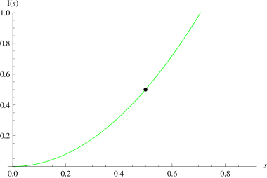
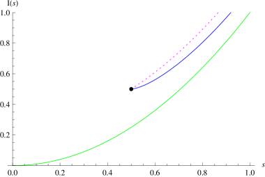
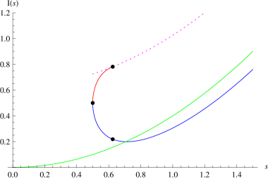
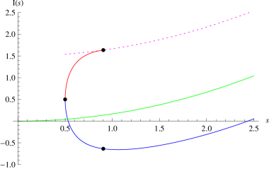
Figure 2: Plots of the free energies $I(s)$ of the different branches for $p=1,2,5,12$, respectively. The first plot is the free energy of the 1/2 BPS Taub-NUT-AdS solution. In the other plots the green curve is the free energy $\tfrac{1}{p}I_{\mathrm{NUT}}$ of the Taub-NUT-AdS$/\mathbb{Z}_{p}$ solution, while the dotted line in magenta is the free energy $I_{\mathrm{NUT+flux}}^{\mathrm{orb}}$, including the contribution of $\pm\frac{p}{2}$ units of flux at the orbifold singularity. The red curve is the free energy $I_{\mathrm{Bolt_{-}}}$ of the negative branch. The blue curve is the free energy $I_{\mathrm{Bolt_{+}}}$ of the positive branch. The free energies of the special solutions are marked with points.

In Figure 2 we have plotted the holographic free energies for various values of $p$. The first plot is the free energy of the unique 1/2 BPS filling of the squashed $S^{3}$, with the marked point being the AdS₄ solution without gauge field. In the second plot $p=2$ and we see that the free energy of the positive branch bolt solution joins at $s=\frac{1}{2}$ to the free energy of the orbifold Taub-NUT-AdS$/\mathbb{Z}_{2}$ solution with $1$ unit of flux at the singularity, as observed in [15]. On the same plot the green curve is the free energy of Taub-NUT-AdS$/\mathbb{Z}_{2}$, without any trapped flux. In the remaining two plots ($p=5$ and $p=12$ respectively) the negative branch bolt solutions appear. The curve of the free energy $I_{\mathrm{Bolt_{-}}}$ connects the free energy $I_{\mathrm{NUT+flux}}^{\mathrm{orbifold}}$ of the orbifold branch with the free energy $I_{\mathrm{Bolt_{+}}}$ of the positive branch at the values $s=s_{p}$ and $s=\frac{1}{2}$, respectively.

5 Regular 1/4 BPS solutions

In this section we find all regular supersymmetric solutions satisfying the 1/4 BPS condition (2.12). For all solutions the (conformal class of the) boundary three-manifold is again a biaxially squashed $S^{3}/\mathbb{Z}_{p}$ with metric (4.1), but now the boundary gauge field is given by

$$A^{(3)} = P\sigma_{3}+A^{(3)}_{\mathrm{flat}}\ =\ -\frac{1}{2}(4s^{2}-1)\sigma_{3}+A^{(3)}_{\mathrm{flat}}~{},$$ (5.1)

where $A^{(3)}_{\mathrm{flat}}$ is again a certain flat connection. The latter is particularly important in order to globally have supersymmetry on the boundary in this case, precisely as for the 1/4 BPS Quaternionic-Eguchi-Hanson solutions in section 3.3.2. The boundary Killing spinor equation is (2.65), which we reproduce here for convenience:

$$\left(\nabla_{\alpha}^{(3)}-\mathrm{i}A_{\alpha}^{(3)}+\frac{\mathrm{i}s}{2}\gamma_{\alpha}\right)\chi = 0~{}.$$ (5.2)

Again as in section 4, a solution to the above boundary data with given $s$ is diffeomorphic to the same solution with $s\rightarrow-s$.

As for the case of 1/2 BPS solutions, for fixed conformal boundary data we find more than one smooth supersymmetric filling, with different topologies. What is exceptional in the 1/4 BPS class of solutions is that for an $S^{3}$ boundary the Taub-NUT-AdS solution is not the unique filling, as one might expect, but rather there is also a filling with an $\mathcal{M}_{1}=\mathcal{O}(-1)\rightarrow S^{2}$ topology. The full moduli space will be summarized in section 5.3.

5.1 Self-dual Einstein solutions

The 1/4 BPS Einstein solutions were described in section 3. For any choice of conformal boundary data, meaning for all $p\in\mathbb{N}$ and all choices of squashing parameter $s>0$, there exists the 1/4 BPS Taub-NUT-AdS solution on $\mathbb{R}^{4}/\mathbb{Z}_{p}$. This has metric (3.5), (3.6) and $\psi$ is taken to have period $4\pi/p$. This solution then has an isolated $\mathbb{Z}_{p}$ orbifold singularity at $r=s$ for $p>1$, or, removing the singularity, the topology is $\mathbb{R}_{>0}\times S^{3}/\mathbb{Z}_{p}$. In taking the $\mathbb{Z}_{p}$ quotient in this 1/4 BPS case notice that in order to preserve supersymmetry we must also turn on an additional flat gauge field which is a connection on $\mathscr{L}^{-1}$. Here recall that $\mathscr{L}$ is the line bundle on $\mathbb{R}_{>0}\times S^{3}/\mathbb{Z}_{p}$ with torsion first Chern class $c_{1}(\mathscr{L})=1\in H^{2}(\mathbb{R}_{>0}\times S^{3}/\mathbb{Z}_{p},\mathbb{Z})\cong\mathbb{Z}_{p}$. The reason for this is as discussed for the Quaternionic-Eguchi-Hanson solutions in section 3.3.2 – the Killing spinors for the 1/4 BPS Taub-NUT-AdS solution are not invariant under $\mathcal{L}_{\partial_{\psi}}$, and the additional torsion gauge field is required in order to have supersymmetry on the quotient space.

On the other hand, for each $p\geq 3$ and specific squashing parameter $s=s_{p}=\tfrac{p}{4\sqrt{p-1}}$ we also have the 1/4 BPS Quaternionic-Eguchi-Hanson solution. Thus for each $p\geq 3$ and $s=s_{p}$ there exist two supersymmetric self-dual Einstein fillings of the same boundary data: the Taub-NUT-AdS solution on $\mathbb{R}^{4}/\mathbb{Z}_{p}$ and the Quaternionic-Eguchi-Hanson solution on $\mathcal{M}_{p}=\mathcal{O}(-p)\rightarrow S^{2}$. Again, the boundary gauge field is important in comparing the global boundary data for these two solutions, and the discussion is essentially the same as for the 1/2 BPS case in section 4.1. In fact the only difference between the two cases is the additional contribution of $\mathscr{L}^{-1}$ described in the previous paragraph.

5.2 Non-self-dual Bolt solutions

5.2.1 Regularity analysis

We begin by analysing when the general metric in (2.6) is regular, where for the 1/4 BPS class the metric function $\Omega(r)=(r-r_{1})(r-r_{2})(r-r_{3})(r-r_{4})$ has roots

$$\left\{\begin{array}[]{c}r_{4}\\ r_{3}\end{array}\right\} = s\pm\sqrt{\frac{-1+2Q+4s^{2}}{2}}~{},$$ (5.5)

$$\left\{\begin{array}[]{c}r_{2}\\ r_{1}\end{array}\right\} = -s\pm\sqrt{\frac{-1-2Q+4s^{2}}{2}}~{}.$$ (5.8)

Again, without loss of generality we may take the conformal boundary to be at $r=+\infty$. A complete metric will then necessarily close off at the largest root $r_{0}$ of $\Omega(r)$, which must satisfy $r_{0}\geq s$. Given (5.5), the largest root is thus either $r_{0}=r_{+}$ or $r_{0}=r_{-}$, where

$$r_{\pm} \equiv \pm s+\sqrt{\frac{-1\pm 2Q+4s^{2}}{2}}~{}.$$ (5.9)

We first note that $r_{0}=r_{\pm}=s$ leads only to the $Q=\mp\frac{1}{2}(4s^{2}-1)$ Taub-NUT-AdS solutions considered in the previous section. Thus $r_{0}>s$ and if $\psi$ has period $4\pi/p$ then the only possible topology is $\mathcal{M}_{p}=\mathcal{O}(-p)\rightarrow S^{2}$. Regularity of the metric near to the $S^{2}$ zero section at $r=r_{0}$ requires, as in the previous section,

$$\left|\frac{r_{0}^{2}-s^{2}}{s\Omega^{\prime}(r_{0})}\right| = \frac{2}{p}~{}.$$ (5.10)

Imposing (5.10) at $r_{0}=r_{+}$ gives

$$Q\ =\ \begin{cases}\ Q_{+}(s)~{},&s>0\\ \\ -Q^{\pm}_{-}(s)~{},&s<0\end{cases}~{},$$ (5.11)

while for $r_{0}=r_{-}$ imposing (5.10) gives

$$Q\ =\ \begin{cases}\ Q^{\pm}_{-}(s)~{},&s>0\\ \\ -Q_{+}(s)~{},&s<0\end{cases}~{}.$$ (5.12)

Here we have defined

$$Q_{+}(s) \equiv \frac{p^{2}-(16s^{2}-p)\sqrt{f^{+}_{p}(s)}}{128s^{2}}~{},$$

$$Q^{\pm}_{-}(s) \equiv -\frac{p^{2}\mp(16s^{2}+p)\sqrt{f^{-}_{p}(s)}}{128s^{2}}~{},$$ (5.13)

and have introduced the polynomials

$$f^{\pm}_{p}(s)\ \equiv\ (16s^{2}\pm p)^{2}-128s^{2}~{}.$$ (5.14)

Similarly to the 1/2 BPS solutions, notice that a solution with given $s>0$ will be equivalent to the corresponding solution with $s\rightarrow-s<0$. This is because $r_{+}(s)=r_{-}(-s)$, which then leads to exactly the same set of roots in (5.5), and thus the same local metric. In addition, $P(-s)=P(s)$ and $Q_{\pm}(s)=Q_{\pm}(-s)$ and hence the gauge field in (2.6) is also invariant. Thus our parametrization of the roots in (5.5) is such that we need only consider $s>0$, which we henceforth assume.

The putative largest root for (5.11) and (5.12), respectively, is

$$r_{+}(Q=Q_{+}(s))\ =\ \frac{p+\sqrt{f^{+}_{p}(s)}}{16s}~{},$$

$$r_{-}(Q=Q^{\pm}_{-}(s))\ =\ \frac{p\mp\sqrt{f^{-}_{p}(s)}}{16s}~{}.$$ (5.15)

The above expressions are real provided $f_{p}^{\pm}(s)$ are positive semidefinite.

Recall that in order to have a smooth metric we require $r_{0}>s$. Imposing this for $r_{0}=r_{+}(Q_{+}(s))$ and $r_{0}=r_{-}(Q_{-}^{\pm}(s))$ is equivalent to determining the range of $s$ for which the functions

$$a_{p}(s) \equiv (p-16s^{2})+\sqrt{f_{p}^{+}(s)}~{},$$

$$b^{\pm}_{p}(s) \equiv (p-16s^{2})\mp\sqrt{f_{p}^{-}(s)}~{},$$ (5.16)

are strictly positive, respectively. In addition, we must verify that (5.2.1) really is the largest root. We thus define

$$c_{p}(s) \equiv r_{+}(Q_{+}(s))-r_{-}(Q_{+}(s))~{},$$

$$d^{\pm}_{p}(s) \equiv r_{-}(Q^{\pm}_{-}(s))-r_{+}(Q^{\pm}_{-}(s))~{},$$ (5.17)

and one finds

$$c_{p}(s)\ =\ \frac{p+16s^{2}+\sqrt{f_{p}^{+}}-\sqrt{(p-16s^{2}-\sqrt{f_{p}^{+}})^{2}-4p^{2}}}{16s}~{},$$ (5.18)

$$d^{\pm}_{p}(s)\ =\ \frac{p-16s^{2}\mp\sqrt{f_{p}^{-}}-\sqrt{(p+16s^{2}\pm\sqrt{f_{p}^{-}})^{2}-4p^{2}}}{16s}~{}.$$ (5.19)

Then (5.2.1) is indeed the largest root provided also $c_{p}(s)$ or $d_{p}^{\pm}(s)$, respectively, is positive or complex.

We are thus reduced to determining the subset of $\{s>0\}$ for which $f_{p}^{\pm}(s)$ is real and non-negative, and, respectively as appropriate, $a_{p}(s)$, $b^{\pm}_{p}(s)$ are strictly positive and $c_{p}(s)$, $d_{p}^{\pm}(s)$ are either strictly positive or complex. We refer to the two sign choices in $r_{\pm}$ as positive and negative branch solutions. The behaviour for $p=1$ and $p=2$ is again qualitatively different from that with $p\geq 3$.

$p=1$

Positive branch

The polynomial $f_{1}^{+}(s)$ is positive semidefinite for $s\in(0,\frac{\sqrt{2}-1}{4}]\cup[\frac{\sqrt{2}+1}{4},\infty)$ but $a_{1}(s)$ is positive only for $s\in(0,\frac{\sqrt{2}-1}{4}]$. In this range $(1-16s^{2}-\sqrt{f_{1}^{+}})^{2}-4$ is negative and so $c_{1}(s)$ is complex; hence $r_{+}(Q_{+}(s))$ is indeed the largest root of $\Omega(r)$. In conclusion, for $s\in(0,\frac{\sqrt{2}-1}{4}]$ and $Q=Q_{+}(s)$ we have a regular 1/4 BPS solution on $\mathcal{M}_{1}=\mathcal{O}(-1)\rightarrow S^{2}$.

Negative branches

The polynomial $f_{1}^{-}(s)$ is positive semidefinite for $s\in(0,\frac{\sqrt{3}-\sqrt{2}}{4}]\cup[\frac{\sqrt{2}+\sqrt{3}}{4},\infty)$ but $b^{\pm}_{1}(s)$ is positive only for $s\in(0,\frac{\sqrt{3}-\sqrt{2}}{4}]$. In this range $(1+16s^{2}\pm\sqrt{f_{1}^{-}})^{2}-4$ is negative and so $d^{\pm}_{1}(s)$ is complex; hence $r_{-}(Q^{\pm}_{-}(s))$ is indeed the largest root of $\Omega(r)$. In conclusion, for $s\in(0,\frac{\sqrt{3}-\sqrt{2}}{4}]$ and $Q=Q^{\pm}_{-}(s)$ we have two regular 1/4 BPS solutions on $\mathcal{M}_{1}=\mathcal{O}(-1)\rightarrow S^{2}$.

$p=2$

Positive branch

For $p=2$ the expressions for $r_{+}(Q_{+}(s))$ and $Q_{+}(s)$ simplify to

$$r_{+}(Q_{+}(s)) = \frac{1}{4s}-s~{},~{}~{}~{}~{}~{}Q_{+}(s)\ =\ \frac{1}{16s^{2}}-\frac{1}{2}+2s^{2}~{}.$$ (5.20)

The above values satisfy (5.10) for $s\in(0,\frac{1}{2\sqrt{2}})$. In this range $a_{2}(s)$ is positive while $c_{2}(s)$ is complex, i.e. $r_{+}(Q_{+}(s))$ is indeed the largest root of $\Omega(r)$. In conclusion, for $s\in(0,\frac{1}{2\sqrt{2}})$ and $Q=Q_{+}(s)$ we have a regular 1/4 BPS solution on $\mathcal{M}_{2}=\mathcal{O}(-2)\rightarrow S^{2}$. In the limit $s=\frac{1}{2\sqrt{2}}$, the root $r_{+}(Q_{+}(s))=s=\frac{1}{2\sqrt{2}}$ which corresponds to a Taub-NUT solution.

Negative branches

The polynomial $f_{2}^{-}(s)$ is positive semidefinite for $s\in(0,\frac{2-\sqrt{2}}{4}]\cup[\frac{\sqrt{2}+2}{4},\infty)$ but $b^{\pm}_{2}(s)$ is positive only for $s\in(0,\frac{2-\sqrt{2}}{4}]$. In this range $(2+16s^{2}\pm\sqrt{f_{2}^{-}})^{2}-16$ is negative and so $d^{\pm}_{2}(s)$ is complex. In conclusion, for $s\in(0,\frac{2-\sqrt{2}}{4}]$ and $Q=Q^{\pm}_{-}(s)$ we have two regular 1/4 BPS solutions on $\mathcal{M}_{2}=\mathcal{O}(-2)\rightarrow S^{2}$.

$p\geq 3$

Positive branch

The polynomial $f_{p}^{+}(s)$ is positive definite for all $s>0$ since it has imaginary roots and $a_{p}(s)$ is also positive for all $s>0$. In this range $c_{p}(s)$ is positive and hence $r_{+}(Q_{+}(s))$ is indeed the largest root of $\Omega(r)$. In conclusion, for $s>0$ and $Q=Q_{+}(s)$ we have a regular 1/4 BPS solution on $\mathcal{M}_{p}=\mathcal{O}(-p)\rightarrow S^{2}$.

Negative branches

The polynomial $f_{p}^{-}(s)$ is positive semidefinite for $s\in(0,\frac{\sqrt{2+p}-\sqrt{2}}{4}]\cup[\frac{\sqrt{2}+\sqrt{2+p}}{4},\infty)$ but $b^{\pm}_{p}(s)$ is positive only for $s\in(0,\frac{\sqrt{2+p}-\sqrt{2}}{4}]$. In this range $d^{\pm}_{2}(s)$ is positive and hence $r_{-}(Q^{\pm}_{-}(s))$ is indeed the largest root of $\Omega(r)$. In conclusion, for $s\in(0,\frac{\sqrt{2+p}-\sqrt{2}}{4}]$ and $Q=Q^{\pm}_{-}(s)$ we have two regular 1/4 BPS solutions on $\mathcal{M}_{p}=\mathcal{O}(-p)\rightarrow S^{2}$.

It is important to remark that these various branches of solutions really are distinct solutions. In particular, one should verify that the two negative branch solutions are not diffeomorphic. We have checked this is this case by comparing the value of the square of the Ricci tensor $R_{\mu\nu}R^{\mu\nu}$ evaluated on the bolt $S^{2}$ at $r=r_{0}$ (this may be defined in a coordinate-independent manner as the fixed point set of $U(1)_{r}$, generated by $\partial_{\psi}$). Indeed, one easily computes the general expression

$$R_{\mu\nu}R^{\mu\nu} = 36+\frac{4(P^{2}-Q^{2})^{2}}{(r^{2}-s^{2})^{4}}~{}.$$ (5.21)

It is a simple exercise to compute this at $r=r_{0}$ for the various cases, and check that the solutions we claim are distinct give distinct values of this curvature invariant on the bolt.

5.2.2 Gauge field and spinors

Let us now turn to analysing the global properties of the gauge field. After a suitable gauge transformation, the latter can be written locally as

$$A = \frac{s}{r^{2}-s^{2}}\left[-2Qr-\frac{1}{2s}(r^{2}+s^{2})(4s^{2}-1)\right]\,\sigma_{3}~{}.$$ (5.22)

In particular, this gauge potential is singular on the $S^{2}$ at $r=r_{0}$, but is otherwise globally defined on the complement $\mathcal{M}_{p}\setminus S^{2}$ of the bolt. The field strength $F=\mathrm{d}A$ is easily verified to be a globally defined smooth two-form on $\mathcal{M}_{p}$, with non-trivial flux through the $S^{2}$ at $r=r_{0}$. Indeed, for $Q=Q_{\pm}(s)$ one computes the period through the $S^{2}$ at $r_{0}(s)=r_{\pm}(Q_{\pm}(s))$ (respectively) to be

$$\int_{S^{2}}\frac{F}{2\pi} = -\frac{2s}{r_{0}(s)^{2}-s^{2}}\left[-2Q_{\pm}(s)r_{0}(s)-\frac{1}{2}(r_{0}(s)^{2}+s^{2})(4s^{2}-1)\right]$$ (5.23)

$$= \pm\frac{p}{2}-1~{}.$$

Thus the positive/negative branch solutions have a gauge field flux $\pm\frac{p}{2}-1$ through the bolt, respectively. Both branches then induce the same spinors and global gauge field at conformal infinity, for fixed $p$ and $s$. The factor of $-1$ in the quantization condition (5.23) is precisely the same as for the 1/4 BPS Quaternionic-Eguchi-Hanson solutions (3.27) in section 3.3.2, and its relation to having globally well-defined spinors on the conformal boundary, invariant under $\mathcal{L}_{\partial_{\psi}}$, is precisely the same as the discussion around equation (3.30).

We note that the Dirac spin^c spinors are smooth sections of the following bundles:

$$\begin{cases}\ \pi^{*}\left[\mathcal{O}(p-2)\oplus\mathcal{O}(0)\oplus\mathcal{O}(-2)\oplus\mathcal{O}(p)\right]&\quad\mbox{positive branch}\\ \ \pi^{*}\left[\mathcal{O}(-2)\oplus\mathcal{O}(-p)\oplus\mathcal{O}(-p-2)\oplus\mathcal{O}(0)\right]&\quad\mbox{negative branch}\end{cases}~{}.$$ (5.24)

When $p$ is even the boundary gauge field $A^{(3)}$ is a connection on $\mathscr{L}^{\frac{p}{2}-1}$, while when $p$ is odd it is a connection on $\mathscr{L}^{-1}$. The three-dimensional boundary spinors are correspondingly sections of $\mathscr{S}_{0}\otimes\mathscr{L}^{-1}$ and $\mathscr{S}\otimes\mathscr{L}^{-1}$, respectively (see appendix D).

5.2.3 Special solutions

For $p<3$ the positive branches described in section 5.2.1 terminate at $s=\frac{\sqrt{2}-\sqrt{2-p}}{4}$ while for $p\geq 3$ the positive branch exists for all $s>0$, but there are special solutions at $s=\tfrac{1}{2}$ and $s=s_{p}$. The negative branches terminate at $\frac{\sqrt{p+2}-\sqrt{2}}{4}$ for all $p$. In this section we describe these various special and/or limiting solutions.

Positive branches

For $p=1$ the positive branch exists for $s\in(0,\tfrac{\sqrt{2}-1}{4}]$. As usual the $s=0$ limit is singular, but the terminating solution with $s=\tfrac{\sqrt{2}-1}{4}$ is a regular solution. At this value of $s$ we have $f^{+}_{1}(s)=0$, although we have not found an invariant geometric interpretation of this characterization of the solution. For $p=2$ the positive branch exists for $s\in(0,\tfrac{1}{2\sqrt{2}})$, but here the terminating solution in the limit $s\rightarrow\tfrac{1}{2\sqrt{2}}$ degenerates to the Taub-NUT-AdS$/\mathbb{Z}_{2}$ solution, which of course has an orbifold singularity. Thus for $p=2$ the positive branch joins onto the Taub-NUT-AdS$/\mathbb{Z}_{2}$ solutions. Notice that, in contrast to the 1/2 BPS case, here the limiting Taub-NUT-AdS$/\mathbb{Z}_{2}$ solution has zero torsion, since $\frac{p}{2}-1=0$ when $p=2$.

For $p\geq 3$ the positive branch exists for all $s>0$, but there are some notable special solutions on this branch. Firstly, $s=\frac{1}{2}$ leads to a round metric on $S^{3}/\mathbb{Z}_{p}$, and thus this solution is a “round Lens filling solution”, as dubbed in section 4. However, while for the 1/2 BPS solutions the round Lens filling solutions were terminating solutions that joined together the positive and negative branches, here it appears as a special point on the positive branch. Of course, it is not a surprise to see the self-dual Quaternionic-Eguchi-Hanson solution arise from the special value $s=s_{p}=\frac{p}{4\sqrt{p-1}}$, and this is another special solution on the $p\geq 3$ 1/4 BPS positive branch.

Negative branches

The negative branches terminate at $s=\frac{\sqrt{p+2}-\sqrt{2}}{4}$ for all $p\geq 1$. At this value of $s$ we have $f^{-}_{p}(s)=0$, and in fact the two negative branches become identical at this point, and thus join together. Again, we have not found a geometrical characterization of the condition that $f^{-}_{p}(s)=0$. Notice that for $p\geq 10$ we have $\tilde{s}_{p}\equiv(\sqrt{p+2}-\sqrt{2})/4>1/2$, and therefore there exist two additional round Lens filling solutions on the negative branches. These are distinct solutions, as follows by comparing the curvature invariant (5.21) on the bolt $S^{2}$.

5.3 Moduli space of solutions

We have summarized the even more intricate branch structure of the 1/4 BPS solutions in Figure 3. In general the conformal boundary has biaxially squashed $S^{3}/\mathbb{Z}_{p}$ metric (4.1), with squashing parameter $s>0$, and boundary gauge field given by (5.1). The 1/4 BPS fillings of this boundary may then be summarized as follows:

• For $p=1$, the boundary $S^{3}$ with arbitrary squashing parameter $s>0$ always has the Taub-NUT-AdS solution as filling, but for $s\in(0,\frac{\sqrt{2}-1}{4}]$ there is also a smooth positive branch solution with topology $\mathcal{M}_{1}=\mathcal{O}(-1)\rightarrow S^{2}$, while for $s\in(0,\frac{\sqrt{3}-\sqrt{2}}{4}]$ there are two negative branch solutions (which are connected to each other) of the same topology. The Taub-NUT, positive, and negative branch solutions are disconnected from each other; this in fact had to be the case, as we shall see in the next section that they have different constant free energy. Notice that the $s=\frac{1}{2}$ AdS₄ metric sits on the Taub-NUT-AdS branch.

• For $p\geq 2$ and arbitrary squashing parameter $s>0$ we always have the (mildly singular) Taub-NUT-AdS$/\mathbb{Z}_{p}$ solution. Thus for all boundary data there always exists a gravity filling, provided one allows for orbifold singularities.

• For $p=2$ there is a positive branch filling for $s\in(0,\frac{1}{2\sqrt{2}})$ with topology $\mathcal{M}_{2}=\mathcal{O}(-2)\rightarrow S^{2}$. This joins onto the Taub-NUT-AdS$/\mathbb{Z}_{2}$ branch at $s=\frac{1}{2\sqrt{2}}$, and we shall indeed see that these have the same free energy. Notice that, since $\frac{p}{2}-1=0$ for $p=2$, the gauge field is a connection on a trivial line bundle. For $s\in(0,\frac{2-\sqrt{2}}{4}]$ there are again two negative branch solutions. These are connected to each other, but disconnected from the positive branch and Taub-NUT-AdS branch.

• For all $p>2$ and $s>0$ there exists a positive branch filling with topology $\mathcal{M}_{p}=\mathcal{O}(-p)\rightarrow S^{2}$. This includes the Quaternionic-Eguchi-Hanson solution at the specific value $s=s_{p}=\frac{p}{4\sqrt{p-1}}$, and the round Lens filling solution at $s=\frac{1}{2}$. However, this positive branch is disconnected from the Taub-NUT-AdS branch. For $s\in(0,\frac{\sqrt{p+2}-\sqrt{2}}{4}]$ there are again two negative branch solutions, which are connected to each other but disconnected from the positive branch and Taub-NUT-AdS branch. For $p\geq 10$ there exist two additional distinct round Lens filling solutions on the negative branches.

  

  Figure 3: The moduli space of 1/4 BPS solutions with biaxially squashed $S^{3}/\mathbb{Z}_{p}$ boundary, with squashing parameter $s$. The arrows denote identification of solutions on different branches. Notice that these moduli spaces are generally disconnected, as follows from the fact that the free energies are different. Note also that the negative branches extend past the round Lens filling solutions at $s=\frac{1}{2}$ only when $p\geq 10$ (which is the case plotted).

5.4 Holographic free energy

In this subsection we compute the holographic free energy of the 1/4 BPS solutions summarized above. This follows similarly section 4.4, thus we will be more brief. Again we refer to appendices E and G for further details. We compute

$$I^{\text{grav}}_{\text{bulk}} = \frac{1}{8\pi G_{4}}\frac{16\pi^{2}}{p}\left.(2sr^{3}-6s^{3}r)\right|_{r_{0}}^{\varrho}~{},$$ (5.25)

$$I^{\text{grav}}_{\text{ct}}+I^{\text{grav}}_{\text{bdry}} = \frac{1}{8\pi G_{4}}\frac{16\pi^{2}}{p}[4Qs^{2}-2s\varrho^{3}+6s^{3}\varrho+\mathcal{O}(\varrho^{-1})]~{},$$ (5.26)

where $r_{0}=r_{\pm}$ is the appropriate largest root of $\Omega(r)$, where the manifold closes off. Removing the cut-off $\varrho\to\infty$ the divergent terms cancel. The contribution to the action from the bulk gauge field is as follows. For the NUT case $r_{0}=s$ and we have

$$I^{F}_{\mathrm{NUT}}\ =\ \frac{16\pi^{2}}{8\pi G_{4}}Q^{2}\ =\ \frac{2\pi}{G_{4}}\frac{(1-4s^{2})^{2}}{4}~{},$$ (5.27)

while for the Taub-Bolt-AdS cases $r_{0}>s$ and we have

$$I^{F}_{\mathrm{Bolt}}\ =\ \frac{1}{8\pi G_{4}}\frac{16\pi^{2}}{p}\frac{sr_{0}\left[-4Q(1-4s^{2})(r_{0}+s)^{2}+(r_{0}^{2}+s^{2})(2Q+1-4s^{2})^{2}\right]}{2(r_{0}^{2}-s^{2})^{2}}~{}.$$ (5.28)

Combining all the above contributions to the action we obtain the following remarkably simple expressions

$$I_{\mathrm{NUT}} \ =\ \frac{1}{2}\frac{\pi}{G_{4}}\qquad\qquad(p=1)~{},$$ (5.29)

$$I_{\mathrm{Bolt\pm}} \ =\ \frac{4\mp p}{8}\frac{\pi}{G_{4}}\qquad~{}(p\geq 2)~{}.$$

Again, $I_{\mathrm{Bolt_{\pm}}}$ refers to the free energies of the positive and negative branch solutions, respectively. In particular, the two distinct (non-diffeomorphic) negative branches in fact have the same free energy, that we denote $I_{\mathrm{Bolt_{-}}}$.

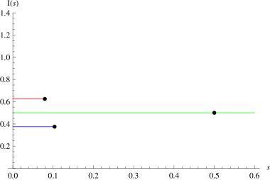
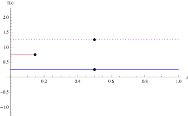
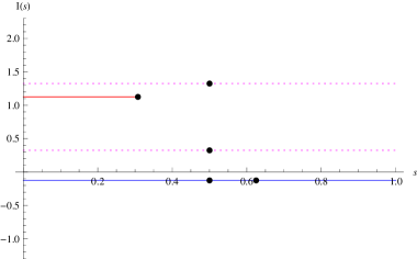
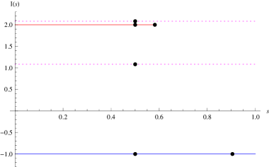
Figure 4: Plots of the free energies $I(s)$ of the different branches for $p=1,2,5,12$, respectively. The dotted lines in magenta are the free energies $I_{\mathrm{NUT+flux_{\pm}}}^{\mathrm{orb}}$, including the contribution of $\pm\frac{p}{2}-1$ units of flux at the orbifold singularity. The red lines are the free energies $I_{\mathrm{Bolt_{-}}}$ of the negative branches. The blue lines are the free energies $I_{\mathrm{Bolt_{+}}}$ of the positive branches. The special solutions are marked with points.

As for the 1/2 BPS solutions, for any $p\geq 2$ we can fill the boundary squashed Lens space $S^{3}/\mathbb{Z}_{p}$ with the 1/4 BPS Taub-NUT-AdS/$\mathbb{Z}_{p}$ solution, where $\mathbb{Z}_{p}$ acts on the coordinate $\psi$. Here we must consider more specifically the orbifold NUT solutions with $\pm\frac{p}{2}-1$ units of flux trapped at the orbifold singularity, as a direct quotient of the Taub-NUT-AdS solution is not supersymmetric. The latter solutions have the same global boundary data as the Taub-Bolt-AdS solutions, and in particular the trapped flux induces the same topological class of the gauge field on the conformal boundary $S^{3}/\mathbb{Z}_{p}$. Using the result of appendix G we compute the total action

$$I_{\mathrm{NUT+flux_{\pm}}}^{\mathrm{orbifold}} = \frac{1}{p}I_{\mathrm{NUT}}+I_{\mathrm{sing}}\ =\ \left(\frac{1}{2p}+\left(\frac{p}{2}\mp 1\right)^{2}\frac{1}{2p}\right)\frac{\pi}{G_{4}}~{},$$ (5.30)

where in this case we obtain two different values depending on the sign of the flux. In Figure 4 we plotted the holographic free energies for various values of $p$. The most striking feature is that we now have four distinct smooth supergravity solutions filling a squashed $S^{3}$ boundary ($p=1$). The corresponding free energies are shown in the first plot.

6 M-theory solutions and holography

In this section we discuss how the four-dimensional supergravity solutions uplift to solutions of eleven-dimensional supergravity. The full eleven-dimensional solution will take the form of a fibration over $\mathcal{M}^{(4)}$, where the fibres are copies of the internal space $Y_{7}$. The choice of the latter determines the field theory dual that is defined on the biaxially squashed $S^{3}/\mathbb{Z}_{p}$ conformal boundary of $\mathcal{M}^{(4)}$. Recall that for all solutions the four-dimensional gauge field $A$ satisfies the quantization condition for a spin^c gauge field, and in particular $2A$ is always a connection on a line bundle $L$ over $\mathcal{M}^{(4)}$. As we shall see, the Taub-NUT-AdS solutions may always be uplifted to global supersymmetric M-theory solutions, for any choice of internal space $Y_{7}$, and in this case we are able to compare the free energies computed in sections 4 and 5 to corresponding large $N$ field theory results, and find agreement in section 6.2. An important point here is that the Taub-NUT-AdS solutions have topology $\mathcal{M}^{(4)}\cong\mathbb{R}^{4}$, so that the line bundle ${L}$ is necessarily topologically trivial, i.e. the four-dimensional graviphoton $A$ is globally a one-form on $\mathcal{M}^{(4)}$. However, as soon as $c_{1}({L})\in H^{2}(\mathcal{M}^{(4)},\mathbb{Z})$ is non-zero this puts constraints on the possible choices of $Y_{7}$ – this is the case for almost all of the Taub-Bolt-AdS solutions, and even the Taub-NUT-AdS$/\mathbb{Z}_{p}$ solutions if they have non-trivial flat connections turned on.

This may be rephrased as follows. Given any supersymmetric field theory with an AdS${}_{4}\times Y_{7}$ gravity dual, this field theory may also be put on the biaxially squashed $S^{3}$, preserving 1/2 or 1/4 supersymmetry. Any such field theory then has a Taub-NUT-AdS filling as a gravity dual, of the form $\mathcal{M}^{(4)}\times Y_{7}$ where $\mathcal{M}^{(4)}$ is the Taub-NUT-AdS solution with appropriate 1/2 BPS or 1/4 BPS instanton, respectively. However, only a certain class of field theories, meaning only certain choices of $Y_{7}$, has in addition the 1/4 BPS Taub-Bolt-AdS filling of section 5. Similar comments apply to the case of the biaxially squashed Lens spaces $S^{3}/\mathbb{Z}_{p}$. We shall describe some choices of corresponding $Y_{7}$ in section 6.4, and comment on the dual field theories.

6.1 Lifting NUTs

As shown in [26], any supersymmetric solution to $d=4$, $\mathcal{N}=2$ gauged supergravity theory uplifts locally to a supersymmetric solution of $d=11$ supergravity. More precisely, given any Sasaki-Einstein seven-manifold $Y_{7}$ with contact one-form $\eta$, transverse Kähler-Einstein metric $\mathrm{d}s^{2}_{T}$ and with the seven-dimensional metric normalized so that $R_{ij}=6g_{ij}$, we have the uplifting ansatz

$$\mathrm{d}s^{2}_{11} = R^{2}\left(\frac{1}{4}\mathrm{d}s^{2}_{4}+\left(\eta+\frac{1}{2}A\right)^{2}+\mathrm{d}s^{2}_{T}\right)~{},$$

$$G = R^{3}\left(\frac{3}{8}\mathrm{vol}_{4}-\frac{1}{4}*_{4}F\wedge\mathrm{d}\eta\right)~{}.$$ (6.1)

Here $\mathrm{d}s^{2}_{4}$ is the four-dimensional gauged supergravity metric on $\mathcal{M}^{(4)}$, with volume form $\mathrm{vol}_{4}$, and the radius $R$ is

$$R^{6} = \frac{(2\pi\ell_{p})^{6}N}{6\mathrm{Vol}(Y_{7})}~{},$$ (6.2)

where $N$ is the number of units of flux

$$N = \frac{1}{(2\pi\ell_{p})^{6}}\int_{Y_{7}}*_{11}G~{}.$$ (6.3)

The four-dimensional Newton constant is then given by

$$\frac{1}{16\pi G_{4}} = N^{3/2}\sqrt{\frac{\pi^{2}}{32\cdot 27\mathrm{Vol}(Y_{7})}}~{}.$$ (6.4)

In fact it was more generally conjectured in [26] that given any $\mathcal{N}=2$ warped AdS${}_{4}\times Y_{7}$ solution of eleven-dimensional supergravity there is a consistent Kaluza-Klein truncation on $Y_{7}$ to $d=4$, $\mathcal{N}=2$ gauged supergravity theory. Properties of such general solutions have recently been investigated in [40, 41], and we expect the contact structure discussed in these references to play an important role in this truncation. In particular, it was shown in [41] that (6.4) remains true in this more general setting, provided one replaces the Riemannian volume $\mathrm{Vol}(Y_{7})$ by the contact volume.

As a specific example we may consider simply $Y_{7}=S^{7}/\mathbb{Z}_{k}$, with the $\mathbb{Z}_{k}$ action along the Hopf fibre of $S^{7}$. In this case $\mathrm{d}s^{2}_{T}$ is the usual Fubini-Study metric on $\mathbb{CP}^{3}$, and $\eta=\mathrm{d}\xi+A_{\mathbb{CP}^{3}}$, where $\xi$ has period $2\pi/k$ and $\mathrm{d}A_{\mathbb{CP}^{3}}$ is the Kähler form on $\mathbb{CP}^{3}$, normalized to have period $2\pi$ through the linearly embedded $\mathbb{CP}^{1}$. In that case $\mathrm{Vol}(S^{7}/\mathbb{Z}_{k})=\pi^{4}/3k$. Different choices of $Y_{7}$ correspond to differerent choices of Chern-Simons-matter theory on the squashed $S^{3}$, and there are by now many examples of dual pairs, including infinite families.

The Taub-NUT-AdS solutions have topology $\mathcal{M}^{(4)}\cong\mathbb{R}^{4}$, and then necessarily $A$ is globally a one-form on $\mathbb{R}^{4}$. It follows immediately from the uplifting formula (6.1) that we obtain a globally supersymmetric eleven-dimensional solution, again of the product topology $\mathcal{M}^{(4)}\times Y_{7}$, for any choice of AdS${}_{4}\times Y_{7}$ solution. Specifically, because $A$ is a global one-form on $\mathcal{M}^{(4)}$, the twisting $\eta+\tfrac{1}{2}A$ is topologically trivial. Notice also that there is no flux quantization condition on $G$, since $\mathrm{d}\eta$ is exact. Thus any supersymmetric field theory on $S^{3}$ with an AdS${}_{4}\times Y_{7}$ dual also has, when the theory is put on the biaxially squashed $S^{3}$, a supersymmetric $(\mbox{Taub-NUT-AdS})\times Y_{7}$ dual, in both the 1/2 BPS and 1/4 BPS cases. We may then compare the gravitational holographic free energies of these solutions to corresponding exact large $N$ field theory computations, which we will do in the next section.

6.2 Comparison to field theory duals

The gravitational holographic free energies of the 1/2 BPS and 1/4 BPS Taub-NUT-AdS solutions were computed in sections 4.4 and 5.4, respectively. The result is

$$I_{\mathrm{NUT}} = \begin{cases}\displaystyle\ \frac{\pi}{2G_{4}}&\quad\mbox{1/4 BPS}\\[11.38109pt] \displaystyle\ \frac{(2s)^{2}\pi}{2G_{4}}&\quad\mbox{1/2 BPS}\end{cases}~{}.$$ (6.5)

Using the formula (6.4) for the four-dimensional Newton constant, we thus obtain

$$I_{\mathrm{NUT}} = \begin{cases}\displaystyle\ \frac{\sqrt{2}\pi}{3}\sqrt{\frac{\mathrm{Vol}(S^{7})}{\mathrm{Vol}(Y_{7})}}N^{3/2}&\quad\mbox{1/4 BPS}\\[11.38109pt] \displaystyle\ (2s)^{2}\frac{\sqrt{2}\pi}{3}\sqrt{\frac{\mathrm{Vol}(S^{7})}{\mathrm{Vol}(Y_{7})}}N^{3/2}&\quad\mbox{1/2 BPS}\end{cases}~{}.$$ (6.6)

In fact the 1/2 BPS case was precisely studied by the authors in [15]. In this case the biaxially squashed $S^{3}$ with metric (2.47), boundary gauge field (2.48) and three-dimensional Killing spinor equation (2.46) was studied in [17]. In the latter reference the authors showed that, for a large class of $\mathcal{N}=2$ Chern-Simons-quiver gauge theories, the leading large $N$ free energy is precisely $(2s)^{2}$ times the result for the round sphere (see equation (148) in [17]). This is precisely what we obtain from the 1/2 BPS Taub-NUT-AdS gravity solution (6.6), which has the same conformal boundary data!

In the 1/4 BPS case the boundary three-metric (2.47) is the same as in the 1/2 BPS case, but the boundary gauge field (2.66) and three-dimensional Killing spinor equation (2.65) are different. General $\mathcal{N}=2$ Chern-Simons-matter theories were studied on this biaxially squashed $S^{3}$ in [16], and it was found that the partition function is independent of the squashing parameter. This is an exact statement, valid for all $N$. This then precisely agrees with our large $N$ gravity result in (6.6), where we find that the gravitational free energy is equal to the result for the round sphere with $s=\frac{1}{2}$. Thus the 1/4 BPS Taub-NUT-AdS solution reproduces the correct large $N$ free energy. Of course, this can only be regarded as a partial result at this stage, because in the 1/4 BPS case there is also the Taub-Bolt-AdS filling, with topology $\mathcal{M}_{1}=\mathcal{O}(-1)\rightarrow S^{2}$. We turn to these solutions next.

6.3 Lifting bolts

The Taub-Bolt-AdS solutions certainly uplift locally to eleven-dimensional supersymmetric supergravity solutions via (6.1). However, globally this uplifting ansatz is inconsistent unless one restricts the internal space $Y_{7}$ appropriately. In this section we explain this important global subtlety. This implies that only a restricted class of field theories have Taub-Bolt-AdS fillings, in addition to the universal Taub-NUT-AdS fillings described in the previous section.

The discussion that follows is entirely topological, and we may in fact treat all of the 1/2 BPS and 1/4 BPS cases simultaneously. Specifically, all that we shall need to know is that the topology of the Taub-Bolt-AdS solutions is $\mathcal{M}^{(4)}=\mathcal{M}_{p}\equiv\mathcal{O}(-p)\rightarrow S^{2}$, with the gauge field flux quantized as

$$\int_{S^{2}}\frac{F}{2\pi} = \frac{n}{2}~{}.$$ (6.7)

In all cases $n\equiv p$ mod 2, which is equivalent to $A$ be a spin^c gauge field, as discussed in detail in appendix D.

For simplicity, we shall consider first the case of uplifting when the internal manifold $Y_{7}$ is a regular Sasaki-Einstein manifold. By definition this means that $Y_{7}$ is the total space of a $U(1)$ principal bundle over a Kähler-Einstein six-manifold $B_{6}$ with metric $\mathrm{d}s^{2}_{T}$. We may then write $\eta=\mathrm{d}\xi+\sigma$, where standard formulae give $\mathrm{d}\sigma=\rho/4$ where $\rho$ is the Ricci-form on $B_{6}$. The canonical period for $\xi$ is then $2\pi/4$, which for a Sasaki-Einstein manifold with precisely two Killing spinors is also the smallest period compatible with supersymmetry: the Killing spinors on $Y_{7}$ are charged under the Reeb vector $\partial_{\xi}$, and taking $\xi$ to have period $2\pi/4m$ for any $m>1$ would lead to spinors that are not single-valued. When $\xi$ has period $2\pi/4$ $Y_{7}$ is in fact the total space of the $U(1)$ principal bundle associated to the anti-canonical line bundle over $B_{6}$. On the other hand, $\xi$ can sometimes have larger period. In fact $Y_{7}$ is simply-connected if and only if $\xi$ has period $2\pi I/4$ where $I=I(B_{6})\in\mathbb{N}$ is a positive integer called the Fano index of $B_{6}$ [42]. In particular, for $B_{6}=\mathbb{CP}^{3}$ we have $I(\mathbb{CP}^{3})=4$, so that for $Y_{7}=S^{7}$ we must take $\xi$ to have period $2\pi$. In fact $I\in\{1,2,3,4\}$, with $I=4$ only for $B_{6}=\mathbb{CP}^{3}$.

We may summarize the previous paragraph, then, by taking $\xi$ to have period $2\pi I/4k$, where $I=I(B_{6})\in\{1,2,3,4\}$ is the Fano index, and the positive integer $k$ must then divide $I$ in order that the two $U(1)_{R}$ charged Killing spinors are single-valued. The number of cases is then very small.

The global restriction on the internal space $Y_{7}$ in the uplifting ansatz (6.1) may then be understood by fixing a point in $B_{6}$ and looking at the corresponding circle bundle over the bolt $S^{2}\subset\mathcal{M}^{(4)}$. Since $\xi$ has period $2\pi I/4k$, it follows from the connection term $\eta+\frac{1}{2}A$ appearing in the metric (6.1) that we will obtain a well-defined circle bundle only if

$$\frac{4k}{2I}\int_{S^{2}}\frac{F}{2\pi} = m\ \in\ \mathbb{Z}$$ (6.8)

is an integer. Geometrically, this integer $m$ is (minus) the first Chern class of the circle bundle, with coordinate $\xi$, integrated over the bolt $S^{2}$. Recalling that $2A$ is a connection on what we called $L\rightarrow\mathcal{M}^{(4)}$, we thus see that the eleven-dimensional circle $\xi$ is twisted by the line bundle $L^{k/I}=\mathcal{O}(m)$ in general, rather than by $L$. When $k=I$ these are the same, which is precisely the case when the internal Sasaki-Einstein manifold $Y_{7}$ is the $U(1)$ principal bundle associated to the anti-canonical bundle over $B_{6}$. Given (6.7), the quantization condition (6.8) is equivalent to

$$nk = mI~{}.$$ (6.9)

This necessary condition is then also sufficient for the eleven-dimensional metric (6.1) to be globally well-defined. Specifically, the eleven-dimensional spacetime is by construction the total space of the circle bundle over $\mathcal{M}_{p}\times B_{6}$ with first Chern class $c_{1}=-m\Phi-\frac{k}{I}c_{1}(B_{6})$, where $\Phi$ is the generator of $H^{2}(\mathcal{M}_{p},\mathbb{Z})\cong\mathbb{Z}$. In the $G$-flux in (6.1) notice that now $\mathrm{d}\eta$ is no longer an exact form on the eleven-dimensional spacetime. In fact its cohomology class is equal to the cohomology class of $-\frac{1}{2}F$. But then $*_{4}F\wedge F$ is proportional to the volume form on $\mathcal{M}_{p}$, which is exact on $\mathcal{M}_{p}$ and thus also is exact on the eleven-dimensional spacetime. It follows that there is no quantization condition on $G$. In appendix D.3 we show that if the eleven-dimensional metric is regular then the eleven-dimensional geometry is always a spin manifold (for all $p$), and the eleven-dimensional Killing spinors are smooth and globally defined.

Taking $k=I$, which leads to the canonical period of $2\pi/4$ for $\xi$, we see that the condition (6.9) is always satisfied. Thus all Taub-Bolt-AdS solutions can be uplifted for all regular Sasaki-Einstein $Y_{7}$ with the canonical period of $2\pi/4$ for $\xi$. This is true for any $p$. Examples are then $Y_{7}=S^{7}/\mathbb{Z}_{4}$, $Y_{7}=V^{5,2}/\mathbb{Z}_{3}$, $Y_{7}=Q^{2,2,2}=Q^{1,1,1}/\mathbb{Z}_{2}$, and $Y_{7}=M^{3,2}$. In this case the Reeb $U(1)$ principal bundle, with fibre coordinate $\xi$, is twisted over the base spacetime $\mathcal{M}^{(4)}$ by the line bundle $L$.

However, more generally (6.9) leads to restrictions. Consider the case of $Y_{7}=S^{7}$, which has $I=4$ and $k=1$. It follows from (6.9) that $n$ is necessarily divisible by $4$. But recall that $n\equiv p$ mod 2, so we see immediately that none of the Taub-Bolt-AdS solutions with $p$ odd can be uplifted on the round seven-sphere! In particular, the 1/4 BPS Taub-Bolt-AdS solution that fills the squashed $S^{3}$ cannot be lifted on $S^{7}$ (nor can it be lifted on $S^{7}/\mathbb{Z}_{2}$, although from the previous paragraph it can be lifted on $S^{7}/\mathbb{Z}_{4}$). Concretely, this means that the 1/4 BPS Taub-Bolt-AdS filling of the squashed $S^{3}$ does not exist for the ABJM theory. We shall discuss this further in section 6.4 below. Other cases may be analysed similarly. For example, again taking $Y_{7}=S^{7}$, which has $I=4$ and $k=1$, the 1/2 BPS solutions have $n=\pm p$, which leads to the restriction $p=\pm 4m$, so that the 1/2 BPS Taub-Bolt-AdS solutions uplift on $S^{7}$ only if $p$ is divisible by 4.

Above we have focused on regular Sasaki-Einstein manifolds $Y_{7}$, but it is straightforward to extend this analysis. Irregular Sasaki-Einstein manifolds have $\partial_{\xi}$ with generically non-closed orbits. This means that the coordinate $\xi$ is not periodically identified over a dense open subset of $Y_{7}$. On the other hand, the expression $\eta+\frac{1}{2}A$ defines a global one-form only if $\xi$ is periodically identified in $\eta=\mathrm{d}\xi+\sigma$. Thus one can never lift any of these bolt solutions on irregular Sasaki-Einstein manifolds.

Finally, we conclude this section by commenting on an equivalent way of seeing the restriction on $Y_{7}$, that perhaps more directly makes contact with the field theory dual description. For simplicity, we again take $Y_{7}$ to be a regular Sasaki-Einstein manifold with Kähler-Einstein base $B_{6}$, Fano index $I=I(B_{6})$ and $\xi$ to have period $2\pi I/4k$. It follows that $Y_{7}$ is the unit circle bundle in $\mathcal{L}=\mathcal{K}^{k/I}$, where $\mathcal{K}$ denotes the canonical line bundle of $B_{6}$. In this notation, scalar BPS operators arise in the dual field theory from holomorphic functions on the metric cone over $Y_{7}$. These correspond to holomorphic sections of $\mathcal{L}^{-t}$, with $t\in\mathbb{N}$ a positive integer. The R-charge of the holomorphic function is then proportional to $t$, namely $R=\lambda t=\frac{2k}{I}t$. However, because of the twisting in (6.1), these holomorphic functions become tensored with sections of a line bundle over the $S^{2}$ bolt. Specifically, in its dependence on $\mathcal{M}_{p}\times B_{6}$, a holomorphic function with R-charge $\frac{2k}{I}t$ becomes a section of $\mathcal{L}^{-t}\otimes\mathcal{O}(tm)\cong\mathcal{L}^{-t}\otimes L^{tk/I}$, where the integer $m$ satisfies (6.9). In the irregular case the holomorphic functions generically have irrational R-charges, which then do not lead to well-defined sections over the $S^{2}$ bolt.

6.4 Comments on field theory duals

We have seen that the 1/4 BPS Taub-Bolt-AdS filling of the biaxially squashed $S^{3}$ uplifts on any regular Sasaki-Einstein manifold with period $2\pi/4$ for $\xi$. Examples are $Y_{7}=S^{7}/\mathbb{Z}_{4},V^{5,2}/\mathbb{Z}_{3},Q^{2,2,2}$ and $M^{3,2}$. Proposals for the corresponding field theory duals have been discussed in [43, 44, 45, 46, 47, 48, 49, 50]. However, the solution does not lift on the simply-connected covering spaces in the first three examples. We begin this section by examining this $p=1$ case, noting that all other Taub-Bolt-AdS solutions fill the biaxially squashed Lens spaces $S^{3}/\mathbb{Z}_{p}$ with $p>1$, and so far in the literature no one has studied $\mathcal{N}=2$ supersymmetric gauge theories in this setting: the 1/2 BPS and 1/4 BPS biaxially squashed spheres were studied in [16], [17], and round Lens spaces $S^{3}/\mathbb{Z}_{p}$ without torsion gauge fields were studied in [37].

6.4.1 $S^{3}$ boundary

We first note that, thus far in the literature, the large $N$ limit of the partition function of the field theory models dual to $Q^{2,2,2}$ or $M^{3,2}$ has only been computed using an ad hoc prescription [51]. The issue is that the proposed field theory duals for these Sasaki-Einstein manifolds are chiral, meaning that the matter representation is not real, and this leads to a more complicated matrix model behaviour. In particular, it is possible that saddle points exist within these models corresponding to the Taub-Bolt-AdS solutions.

The $S^{7}/\mathbb{Z}_{4}$ case is also intriguing. Naively one might identify the field theory dual in this case with the ABJM model with $k=4$; afterall, the ABJM theory is a $U(N)_{k}\times U(N)_{-k}$ Chern-Simons-matter theory that is dual to the case $Y_{7}=S^{7}/\mathbb{Z}_{k}$. However, the problem is quite subtle. The central issue is that the $\mathbb{Z}_{k}\subset U(1)$ quotient in the ABJM theory generally leaves $\mathcal{N}=6$ supersymmetry unbroken, but the $U(1)$ R-symmetry that is being gauged when the theory is put on the squashed sphere corresponds to an $\mathcal{N}=2$ subalgebra of this $\mathcal{N}=6$. For the Taub-NUT-AdS solutions we may take $Y_{7}=S^{7}/\mathbb{Z}_{k}$ and identify the $\xi$ circle in the uplifting ansatz (6.1) with a $U(1)_{R}\subset SO(6)$. Here the $\mathbb{Z}_{k}$ quotient is not contained in this $SO(6)$, where the latter rotates the $\mathcal{N}=6$ supercharges in the vector representation. We are then gauging the manifest $U(1)_{R}$ symmetry of the ABJM when viewed in $\mathcal{N}=2$ language. However, this does not work for the Taub-Bolt-AdS solutions on $\mathcal{M}_{1}=\mathcal{O}(-1)\rightarrow S^{2}$, because we are forced to take $\xi$ to have period $2\pi/4$, i.e. the Taub-Bolt-AdS solutions are then defined with internal space $Y_{7}=S^{7}/\mathbb{Z}_{k}\times\mathbb{Z}_{4}$. A dual field theory for the latter is then unknown (it is not simply an orbifold of the ABJM theory).

Of course, one might instead directly identify the $\mathbb{Z}_{k}$ quotient in the ABJM theory with with $\xi$ direction in the uplift (6.1). This then forces $k=4$ for the Taub-Bolt-AdS solutions, and we are gauging a $U(1)_{R}$ symmetry that is not contained in the manifest $\mathcal{N}=6$ supersymmetry of the ABJM theory with $k=4$. This statement might puzzle some readers, since in the literature it is claimed that the ABJM theory has $\mathcal{N}=6$ supersymmetry for all $k>2$, while only $k=1$ and $k=2$ have enhanced $\mathcal{N}=8$ supersymmetry. In fact this is incorrect, but subtly so. In fact there are 8 Killing spinors on $S^{7}/\mathbb{Z}_{k}$ for $k=1,2$ and $k=4$, but for $k=4$ the 2 additional Killing spinors are sections of a different spin bundle to the $\mathcal{N}=6$ Killing spinors that exist on $S^{7}/\mathbb{Z}_{k}$ for all $k$. Recall that spin bundles on a manifold $\mathcal{M}$ are in general classified by $H^{1}(\mathcal{M},\mathbb{Z}_{2})$, and in the case at hand notice that $H^{1}(S^{7}/\mathbb{Z}_{4},\mathbb{Z}_{2})\cong\mathbb{Z}_{2}$. The $\mathcal{N}=6$ spinors are sections of one of these two spin bundles, while the $\mathcal{N}=2$ Killing spinors that exist when $S^{7}/\mathbb{Z}_{4}$ is viewed as a regular Sasaki-Einstein manifold over $\mathbb{CP}^{3}$ are sections of the other spin bundle. Thus although there are 8 Killing spinors, there is not an $SO(8)$ R-symmetry that rotates them. In the field theory we are then gauging this non-manifest $\mathcal{N}=2$ $U(1)_{R}$ symmetry that exists only when $k=4$, which seems rather hard to study in practice.

The conclusion of this is that the internal spaces $Y_{7}$ for which the 1/4 BPS Taub-Bolt-AdS filling of $S^{3}$ exists do not currently have known field theory duals for which the large $N$ partition function computation is under good control: either the field theory models are chiral, and the large $N$ limit of the partition function is correspondingly not well-understood, or no field theory model is currently known, or the field theory is known and non-chiral, but we are gauging a classically non-manifest R-symmetry of that field theory.

6.4.2 $S^{3}/\mathbb{Z}_{p}$ boundary

Let us now turn to the Lens space solutions for $p>1$. Since in general there are a number of distinct cases to consider, we shall confine ourselves to commenting on what we believe are the more interesting cases/features.

Let us first discuss the solutions relevant for the ABJM model: in this case $Y_{7}=S^{7}$ and correspondingly we have $I=4$, $k=1$, and hence $\lambda=\frac{1}{2}$. The latter is indeed the value of the R-charge of a chiral field in the ABJM field theory (these fields are usually called $A_{1},A_{2},B_{1},B_{2}$), and the R-charges of gauge-invariant scalar chiral primary operators are $t/2$, where geometrically $t$ is the positive integer of section 6.3 (these operators are constructed using monopole operators of zero R-charge). Let us focus on the 1/2 BPS class of M-theory solutions. In this case, the Taub-Bolt-AdS solutions have globally distinct boundary conditions, as M-theory solutions, from the corresponding Taub-NUT-AdS$/\mathbb{Z}_{p}$ solution. To see this, note that from (6.9), and using $n=\pm p$, we see that a 1/2 BPS Taub-Bolt-AdS solution uplifts on $S^{7}$ only if $p=4q$ is divisible by 4. In this case, $S^{7}$ is fibred over the base $\mathcal{M}_{p}$ by twisting the Hopf $S^{1}$ bundle by the line bundle $\mathcal{O}(m)=\mathcal{O}(\pm q)$. Alternatively, and equivalently, we may describe the total M-theory spacetime as the total space of the $U(1)$ principal bundle over $\mathcal{M}_{p}\times\mathbb{CP}^{3}$ with first Chern class $c_{1}=\mp q\Phi-H$, where recall that $\Phi$ generates $H^{2}(\mathcal{M}_{p},\mathbb{Z})\cong\mathbb{Z}$ and $H$ is the hyperplane class generating $H^{2}(\mathbb{CP}^{3},\mathbb{Z})\cong\mathbb{Z}$. However, since $\pm q\not\equiv 0$ mod $p=4q$, this $U(1)$ principal bundle is also non-trivially fibred over the boundary Lens space $S^{3}/\mathbb{Z}_{p}$. On the other hand, the Taub-NUT-AdS$/\mathbb{Z}_{p}$ solution is always trivially fibred.

To see what this means in terms of the dual boundary field theory, recall from the discussion at the end of section 6.3 that the functions on $S^{7}$ also become non-trivially fibred over $\mathcal{M}_{p}$ via the twisting, and in particular the Kaluza-Klein modes that are dual to the four chiral fields of the ABJM (or rather their gauge-invariants constructed using monopole operators), become sections of $\mathcal{O}(\pm q)$. This implies that for the Taub-Bolt-AdS solutions these basic matter fields are twisted via their R-charge, becoming sections of $\mathscr{L}^{q}$ rather than functions. We have attempted to study precisely this twisting in the 1/2 BPS case with $s=\frac{1}{2}$, since this is then (conjecturally) simply a twisted version of matrix model studied in [37]. It is straightforward to see that this twisting does indeed preserve supersymmetry, and that localization goes through similarly to the untwisted case. Our results so far are somewhat inconclusive: the behaviour of the matrix model is now much more involved, although interestingly we find that the Wilson loop VEV, discussed in appendix F, is indeed exactly zero, thus agreeing with the gravity prediction. We also find $N^{3/2}$ scaling of the free energy at large $N$, but with a coefficient that doesn’t seem to match the gravity prediction of section 4.4. However, a key issue that affects both this example, and indeed all of the Taub-Bolt-AdS examples, is whether the (potential) twisting of the matter fields by their R-charge is the only effect on the Lagrangian of the untwisted theory, or whether the correct dual field theory is a more complicated deformation. For now we leave this issue open.

Having discussed an example where $I\neq k$, let us conclude this section with the class of Taub-Bolt-AdS solutions where the Sasaki-Einstein manifold has $k=I$, which then all uplift to M-theory. In this case notice that the circle bundle $\xi$ is twisted over the base $\mathcal{M}^{(4)}$ by the line bundle $L$. For the 1/2 BPS solutions this has first Chern class $\pm p$ through the bolt, implying that $L$ restricted to the boundary $S^{3}/\mathbb{Z}_{p}$ is always trivial in this 1/2 BPS class. This implies that all the 1/2 BPS solutions filling a fixed squashed $S^{3}/\mathbb{Z}_{p}$ in fact have the same global boundary data. In turn, in the dual field theory we then don’t have the twisting by the flat R-symmetry Wilson line, discussed in the previous paragraph for the ABJM case. If the field theory Lagrangians are exactly the same in all cases, one should then compare the free energies of all the solutions plotted in Figure 2. However, to our knowledge all field theories within this class are chiral models, for which the matrix model is not under good control.

7 Discussion

In this paper we have presented all supersymmetric asymptotically locally AdS₄ solutions of Euclidean Einstein-Maxwell theory, possessing $SU(2)\times U(1)$ symmetry. We have shown that in general these solutions have one modulus, which is the squashing parameter $s$ of the Lens space metric at conformal infinity. However, we have also uncovered an intricate moduli space of solutions, comprising different branches, joining at special values of the parameter. Perhaps surprisingly, we found that typically for fixed conformal boundary data there exist multiple solutions, with different topologies. We studied global aspects of these solutions, finding a subtle interplay between bulk and boundary spin structures,

We showed that the Taub-Bolt-AdS solutions, despite being perfectly smooth and globally well-defined in four dimensions, can be uplifted to eleven-dimensional supergravity only for particular internal Sasaki-Einstein manifolds. Moreover, we showed that in these solutions the gauge field in the bulk induces non-zero gauge field on the boundary, whose global properties are intimately related to the specific Sasaki-Einstein manifold in the eleven-dimensional solution. Therefore, generically, the supersymmetric Taub-NUT-AdS solutions (and their orbifolds) are the only supersymmetric solutions filling a biaxially squashed Lens space. In particular, there exist only two distinct choices of instantonic gauge field such that the solutions preserve 1/2 or 1/4 supersymmetry, respectively. Following [15, 14], we have argued that these correspond to the two different constructions of supersymmetric field theories on a biaxially squashed three-sphere discussed in [17] and [16], respectively.

Nevertheless, there exist many examples where the Taub-Bolt-AdS solutions exist as global, smooth supersymmetric solutions of eleven-dimensional supergravity. In particular, we have shown that there exist (infinitely many) examples where fixed boundary data can be filled, supersymmetrically, with bulk solutions with different topologies, and with different holographic free energies. In order to address the problem of holographic dual field theories systematically, an important problem that remains open is the possible existence of further M-theory solutions, with the same boundary data as those we have found, but with smaller gravitational free energies. At present we can’t exclude that such solutions exist outside the ansatz that leads to minimal gauged supergravity; for example, there could be supersymmetric solutions with scalar “hair” in the bulk.

We have argued that at least in certain cases (in particular for the ABJM model), the presence of a non-trivial torsion gauge field on the boundary should correspond in the dual field theory to coupling the field theory to a non-trival R-symmetry Wilson line. Although in general this is quite complicated, it may be possible to understand the large $N$ matrix model in the special case when the Lens space metric becomes round ($s=\tfrac{1}{2}$). The corresponding matrix model should then be a twisted version of that studied in [37]. Comparing our gravity predictions to some field theory calculations would be extremely interesting, and could teach us something new about supersymmetric field theories on curved manifolds.

Acknowledgments

We would like to thank Juan Maldacena for inspiring comments on preliminary notes, and Kostas Skenderis for discussions on holographic renormalization of the Einstein-Maxwell theory. We would also very much like to thank Fernando Alday for collaboration on a project addressing a specific question raised in the paper. D. M. would like to thank the Simons Center for Geometry and Physics for hospitality during the 10th Simons Workshop in Mathematics and Physics. D. M. is supported by an EPSRC Advanced Fellowship EP/D07150X/3 and also acknowledges partial support from the STFC grant ST/J002798/1. A.P. is supported by an A.G. Leventis Foundation grant, an STFC studentship and via the Act “Scholarship Programme of S.S.F. by the procedure of individual assessment, of 2011-12” by resources of the Operational Programme for Education and Lifelong Learning, of the European Social Fund (ESF) and of the NSRF, 2007-2013. J. F. S. is supported by the Royal Society and Oriel College.

Appendix A Solving the Einstein-Maxwell equations

In this section we find the general solution to Einstein-Maxwell equations (2) with $SU(2)\times U(1)$ symmetry. The ansatz for the metric and gauge field takes the form

$$\mathrm{d}s^{2}_{4} = \alpha^{2}(r)\mathrm{d}r^{2}+\beta^{2}(r)(\sigma_{1}^{2}+\sigma_{2}^{2})+\gamma^{2}(r)\sigma_{3}^{2}~{},$$

$$A = h(r)\sigma_{3}~{},$$ (A.1)

where $\sigma_{1},\sigma_{2},\sigma_{3}$ are left-invariant one-forms for $SU(2)$, given explicitly by (2.5). In the following analysis we will use the local orthonormal frame

$$\hat{e}^{1}\ =\ \beta(r)\mathrm{d}\theta~{},~{}~{} \hat{e}^{2}\ =\ \beta(r)\sin\theta\mathrm{d}\phi~{},$$ (A.2)

$$\hat{e}^{3}\ =\ \gamma(r)(\mathrm{d}\psi+\cos\theta\mathrm{d}\phi)~{},~{}~{} \hat{e}^{4}\ =\ \alpha(r)\mathrm{d}r~{},$$

and introduce frame indices $a,b,c=1,2,3,4$. The Einstein equations read (with $\ell=1$)

$$R_{ab} = -3\delta_{ab}+2T_{ab}~{},$$ (A.3)

where $T_{ab}=F_{a}{}^{c}F_{bc}-\frac{1}{4}F^{2}\,\delta_{ab}$ is the stress-energy tensor of the gauge field. For the ansatz (A) we compute

$$R_{44} \ =\ -\frac{\gamma^{\prime\prime}}{\alpha^{2}\gamma}+\frac{\alpha^{\prime}\gamma^{\prime}}{\alpha^{3}\gamma}-\frac{2\beta^{\prime\prime}}{\alpha^{2}\beta}+\frac{2\alpha^{\prime}\beta^{\prime}}{\alpha^{3}\beta}~{},$$

$$R_{33} \ =\ -\frac{\gamma^{\prime\prime}}{\alpha^{2}\gamma}+\frac{\alpha^{\prime}\gamma^{\prime}}{\alpha^{3}\gamma}-\frac{2\beta^{\prime}\gamma^{\prime}}{\alpha^{2}\beta\gamma}+\frac{\gamma^{2}}{2\beta^{4}}~{},$$

$$R_{11}\ =\ R_{22} \ =\ -\frac{\beta^{\prime\prime}}{\alpha^{2}\beta}+\frac{\alpha^{\prime}\beta^{\prime}}{\alpha^{3}\beta}-\frac{\beta^{\prime}\gamma^{\prime}}{\alpha^{2}\beta\gamma}-\frac{\beta^{\prime 2}}{\alpha^{2}\beta^{2}}+\frac{1}{\beta^{2}}-\frac{\gamma^{2}}{2\beta^{4}}~{},$$

$$T_{11} \ =\ T_{22}\ =\ -T_{33}\ =\ -T_{44}\ =\ \frac{1}{2}\frac{h^{2}}{\beta^{4}}-\frac{1}{2}\frac{h^{\prime 2}}{\alpha^{2}\gamma^{2}}~{},$$ (A.4)

where a prime denotes derivative with respect to $r$. Furthermore, the equation of motion of the gauge field $\mathrm{d}*F=0$ becomes

$$-\left(\frac{\beta^{2}}{\alpha\gamma}h^{\prime}\right)^{\prime}+\frac{\alpha\gamma}{\beta^{2}}h = 0~{}.$$ (A.5)

By considering the difference $R_{44}-R_{33}$ we obtain the equation

$$-\frac{2\beta^{\prime\prime}}{\alpha^{2}\beta}+\frac{2\beta^{\prime}}{\alpha^{2}\beta}\left(\frac{\alpha^{\prime}}{\alpha}+\frac{\gamma^{\prime}}{\gamma}\right)-\frac{\gamma^{2}}{2\beta^{4}} = 0~{},$$ (A.6)

and by an appropriate reparametrization of $r$ we can take

$$\alpha\gamma = 2s~{},~{}~{}~{}~{}\beta^{2}\ =\ r^{2}-s^{2}~{}.$$ (A.7)

The equation of motion for the gauge field then becomes an ordinary differential equation for $h(r)$:

$$-((r^{2}-s^{2})h^{\prime})^{\prime}+\frac{4s^{2}}{r^{2}-s^{2}}h = 0~{}.$$ (A.8)

The general solution to (A.8) is easily found to be

$$h(r) = P\frac{r^{2}+s^{2}}{r^{2}-s^{2}}-Q\frac{2rs}{r^{2}-s^{2}}~{},$$ (A.9)

where $P$ and $Q$ are integration constants. Substituting this back into the $33$-component of the Einstein equation gives a second order ODE for the metric function $\gamma(r)$. The general solution to this is

$$\gamma^{2}(r) = \frac{4s^{2}}{r^{2}-s^{2}}\left[P^{2}-Q^{2}-2Mr+r^{2}(r^{2}-3s^{2})+C\left(1+\frac{r^{2}}{s^{2}}\right)\right]~{},$$ (A.10)

where $C$ and $M$ are two new integration constants. Substituting this into the $11$-component of the Einstein equations then constrains

$$C = s^{2}(1-3s^{2})~{}.$$ (A.11)

This is precisely an analytic continuation the Reissner-Nordström-Taub-NUT-AdS (RN-TN-AdS) solution in [32]. Hence we have proven that this is the most general solution to the Einstein-Maxwell equations with $SU(2)\times U(1)$ symmetry.

Appendix B Integrability and BPS equations

In this appendix we compute the general integrability conditions for supersymmetry for the Euclidean RN-TN-AdS solutions derived in appendix A. An analysis for Lorentzian solutions was performed in [32].

The Euclidean RN-TN-AdS solutions are given by (2.6), (2.7). In this section we use the orthonormal frame $e^{a}$ in (2.14), which we note is different to the orthonormal frame $\hat{e}^{a}$ used in appendix A, and take the basis of gamma matrices (2.20). The integrability condition for the Killing spinor equation (2.3) reads

$$\mathcal{I}_{ab}\,\epsilon\ =\ 0~{},$$ (B.1)

where

$$\mathcal{I}_{ab} \equiv \frac{1}{4}R_{ab}^{\ \ \ cd}\Gamma_{cd}+\frac{1}{2}\Gamma_{ab}-\mathrm{i}F_{ab}\mathbb{I}_{4}+\frac{\mathrm{i}}{2}\nabla_{[a}F_{|\,cd}\Gamma^{cd}_{\ \ |}\Gamma_{b]}+\frac{\mathrm{i}}{4}\Gamma_{[a}F_{|\,cd}\Gamma^{cd}_{\ \ |}\Gamma_{a]}$$ (B.2)

$$-\frac{1}{16}\left[F_{cd}\Gamma^{cd}\Gamma_{a},F_{cd}\Gamma^{cd}\Gamma_{b}\right]+\frac{\mathrm{i}}{4}F_{cd}\Gamma^{cd}\Gamma_{ab}~{},$$

is a two-form with values in the Clifford algebra.

A necessary condition to have a non-trivial solution to (B.1) is that

$$\det{\!}_{\mathrm{Cliff}}\,\mathcal{I}_{ab} = 0~{},$$ (B.3)

holds for all $a,b$. We compute

$$\det{\!}_{\mathrm{Cliff}}\,\mathcal{I}_{ab} = \frac{-B_{+}B_{-}+D(B_{+}-B_{-})r+D^{2}r^{2}}{(r^{2}-s^{2})^{6}}W_{ab}~{},$$ (B.4)

where

$$D \equiv 2\left[MP-sQ(1-4s^{2})\right]~{},$$

$$B_{\pm} \equiv (M\pm sQ)^{2}-s^{2}(1\pm P-4s^{2})^{2}-(1\pm 2P-5s^{2})(P^{2}-Q^{2})~{},$$ (B.5)

and

$$\left(W_{ab}\right) \equiv \left(\begin{array}[]{cccc}0&1&\frac{1}{16}&\frac{1}{16}\\ 1&0&\frac{1}{16}&\frac{1}{16}\\ \frac{1}{16}&\frac{1}{16}&0&1\\ \frac{1}{16}&\frac{1}{16}&1&0\end{array}\right)~{}.$$ (B.10)

We thus conclude that a necessary condition to have a supersymmetric solution is that the numerator in (B.4) is zero, which is equivalent to

$$D\ =\ 0~{},\qquad B_{+}B_{-}\ =\ 0~{}.$$ (B.11)

These can also be obtained from an analytic continuation [14] of the integrability conditions in [32], but here we have derived the equations from first principles. We study the general solutions to (B.11) in section 2.2.

Appendix C Class III and supersymmetry

In this appendix we show that the condition $P=\pm Q$ characterizing Class III is not sufficient for supersymmetry, but rather the existence of a Killing spinor requires in addition

$$P\ = \ -\frac{1}{2}(4s^{2}-1)~{},\ \ \ \ \text{or}$$

$$P\ = \ -s\sqrt{4s^{2}-1}~{}.$$ (C.1)

In order to prove this we look at the boundary Killing spinor equation, which can be derived from (2.3) upon expanding in powers of $1/r$. At lowest order we find

$$(\nabla^{(3)}_{\alpha}-\mathrm{i}A^{(3)}_{\alpha})\chi-\frac{\mathrm{i}s}{2}\gamma_{\alpha}\chi+\mathrm{i}V_{\beta}\gamma_{\alpha}\gamma^{\beta}\chi\ =\ 0~{}.$$ (C.2)

Here $\nabla^{(3)}$ denotes the spin connection for the three-metric

$$\mathrm{d}s^{2}_{3} = \sigma_{1}^{2}+\sigma_{2}^{2}+4s^{2}\sigma_{3}^{2}~{},$$ (C.3)

with $\gamma_{\alpha}$, $\alpha=1,2,3$ generating the corresponding Cliff$(3,0)$ algebra, and $\chi$ is a two-component spinor. Furthermore

$$A^{(3)} = \lim_{r\rightarrow\infty}A\ =\ P\sigma_{3}~{},$$

$$V = \frac{s^{2}(4s^{2}-1)}{Q}\sigma_{3}~{}.$$ (C.4)

The integrability condition for (C.2) reads

$$\mathcal{I}^{(3)}_{\alpha\beta}\chi\ =\ 0~{},$$ (C.5)

where

$$\begin{split}\mathcal{I}^{(3)}_{\alpha\beta}\ \equiv\ &\frac{1}{4}R^{(3)}_{\alpha\beta}{}^{\alpha_{1}\alpha_{2}}\gamma_{\alpha_{1}\alpha_{2}}-\mathrm{i}F^{(3)}_{\alpha\beta}-\frac{s^{2}}{2}\gamma_{\alpha\beta}-2\mathrm{i}\nabla_{[\alpha|}V_{\alpha_{1}}\gamma_{|\beta]}\gamma^{\alpha_{1}}\\ &-2s\gamma_{[\alpha}V_{\beta]}+2V^{\alpha_{1}}V_{\alpha_{1}}\gamma_{\alpha\beta}-4V_{\alpha_{1}}\gamma_{[\alpha}V_{\beta]}\gamma^{\alpha_{1}}~{}.\end{split}$$ (C.6)

A necessary condition to have a non-trivial solution to (C.5) is that

$$\det{\!}_{\mathrm{Cliff}}\,\mathcal{I}^{(3)}_{\alpha\beta} = 0~{}.$$ (C.7)

Taking into account $P=\pm Q$ we find that this is equivalent to

$$\frac{[(1-4s^{2})^{2}-4Q^{2}][Q^{2}+s^{2}(1-4s^{2})]^{2}}{4Q^{4}}\ =\ 0~{},$$ (C.8)

and hence (C) must hold.

Appendix D Spin^c structures on bolt solutions

In this appendix we discuss in detail the spin^c structures, in the bulk and on the conformal boundary, for the bolt-type solutions. This is a little subtle, because for $p$ odd the bolt solutions are not spin manifolds (but nevertheless are supersymmetric and admit Killing spinors). Correlated with this, the four-dimensional graviphoton in the bulk is in general a spin^c connection, meaning that when $p$ is odd it is not a gauge field in the usual sense. We begin in section D.1 with a general topological discussion, and then in section D.2 give some more explicit details in the cases of interest. Section D.3 contains a brief discussion of lifting these spinors to eleven dimensions.

D.1 Topological discussion

In general, recall that on an orientable four-manifold $\mathcal{M}^{(4)}$ the spin bundle $\mathcal{S}=\mathcal{S}_{+}\oplus\mathcal{S}_{-}$ exists if and only if the second Stiefel-Whitney class is zero, so $w_{2}(\mathcal{M}^{(4)})=0\in H^{2}(\mathcal{M}^{(4)},\mathbb{Z}_{2})$. However, it is also true that on every four-manifold the spin^c bundles $\mathcal{S}_{\pm}\otimes L^{1/2}$ exist, where $L$ is a line bundle satisfying

$$c_{1}(L) \equiv w_{2}(\mathcal{M}^{(4)})\ \ \mbox{mod}\ 2~{}.$$ (D.1)

A spin^c gauge field then has the property that $2A$ is a connection on $L$, so that (formally) $A$ is a connection on $L^{1/2}$.

Recall that the bolt-type solutions all have the topology $\mathcal{M}^{(4)}=\mathcal{M}_{p}=$ total space of $\mathcal{O}(-p)\rightarrow S^{2}$. A simple computation shows that $w_{2}(\mathcal{M}_{p})$ is zero for $p$ even, while for $p$ odd $w_{2}(\mathcal{M}_{p})$ generates the cohomology group $H^{2}(\mathcal{M}_{p},\mathbb{Z}_{2})\cong\mathbb{Z}_{2}$. We assume that the gauge field has field strength $F$ satisfying

$$\int_{S^{2}}\frac{F}{2\pi} = \frac{n}{2}~{},$$ (D.2)

where $S^{2}\subset\mathcal{M}_{p}$ denotes the bolt/zero-section, so that $c_{1}(L)=n\in H^{2}(\mathcal{M}_{p},\mathbb{Z})\cong\mathbb{Z}$. Then via (D.1), we see that $A$ is a spin^c gauge field if and only if $n\equiv p$ mod 2. Notice that for all the solutions discussed in the main text regularity of the metric fixes the gauge field, and that $n\equiv p$ mod 2 was then indeed found to hold automatically for this gauge field. This is a necessary condition for supersymmetry.

In this section we would like to describe the spin^c bundles $\mathcal{S}_{\pm}\otimes L^{1/2}$ more explicitly. We begin by noting that, although the metrics on $\mathcal{M}_{p}$ are not Kähler, nevertheless $\mathcal{M}_{p}$ admits a Kähler structure. We may then use the fact that on a Kähler four-manifold the spin bundles are (formally)

$$\mathcal{S}_{+} = K^{1/2}\oplus K^{-1/2}~{},$$

$$\mathcal{S}_{-} = K^{1/2}\otimes\Omega^{0,1}~{}.$$ (D.3)

Here $K$ denotes the canonical line bundle, while $\Omega^{0,1}$ denotes the holomorphic tangent bundle. The spin bundles (D.1) exist if and only if the square root $K^{1/2}$ exists. A natural choice for $L$ on a Kähler manifold is thus $L=K^{-1}$. If we denote $\pi:\mathcal{M}_{p}\rightarrow S^{2}$ as the projection onto the bolt/zero-section, then for the natural complex structure on $\mathcal{M}_{p}$ implied by our notation we have

$$K = \pi^{*}\mathcal{O}(p-2)~{}.$$ (D.4)

We thus see that $K^{1/2}$ indeed exists if and only if $p$ is even. The spinor bundles are (formally when $p$ is odd) hence

$$\mathcal{S}_{+} = \pi^{*}\left[\mathcal{O}(\tfrac{p}{2}-1)\oplus\mathcal{O}(-\tfrac{p}{2}+1)\right]~{},$$

$$\mathcal{S}_{-} = \pi^{*}\left[\mathcal{O}(-\tfrac{p}{2}-1)\oplus\mathcal{O}(\tfrac{p}{2}+1)\right]~{}.$$ (D.5)

Since $L=\pi^{*}\mathcal{O}(n)$ by definition, we thus compute the spin^c bundles

$$\mathcal{S}_{+}\otimes L^{1/2} = \pi^{*}\left[\mathcal{O}(\tfrac{n+p}{2}-1)\oplus\mathcal{O}(\tfrac{n-p}{2}+1)\right]~{},$$

$$\mathcal{S}_{-}\otimes L^{1/2} = \pi^{*}\left[\mathcal{O}(\tfrac{n-p}{2}-1)\oplus\mathcal{O}(\tfrac{n+p}{2}+1)\right]~{}.$$ (D.6)

In particular, notice that since $n\equiv p$ mod 2, these bundles always exist on $\mathcal{M}_{p}$, as advertised. The Dirac spinors on our bolt solutions are globally sections of the bundles $\mathcal{S}\otimes L^{1/2}=\left(\mathcal{S}_{+}\otimes L^{1/2}\right)\oplus\left(\mathcal{S}_{-}\otimes L^{1/2}\right)$, where the factors are given by (D.1) and $n$ is the flux number given by (D.2). Notice we have made use of (D.1) in the main text, for example to deduce (3.29).

Now we consider how these spinors restrict to the conformal boundary $S^{3}/\mathbb{Z}_{p}=\partial\mathcal{M}_{p}$. Denote the inclusion of this boundary as $\iota:S^{3}/\mathbb{Z}_{p}\hookrightarrow\mathcal{M}_{p}$. Then $H^{2}(S^{3}/\mathbb{Z}_{p},\mathbb{Z})\cong H_{1}(S^{3}/\mathbb{Z}_{p},\mathbb{Z})\cong\mathbb{Z}_{p}$, and the map

$$\mathbb{Z}\ \cong\ H^{2}(\mathcal{M}_{p},\mathbb{Z})\ \stackrel{{\scriptstyle\iota^{*}}}{{\longrightarrow}}\ H^{2}(S^{3}/\mathbb{Z}_{p},\mathbb{Z})\ \cong\ \mathbb{Z}_{p}$$ (D.7)

is simply reduction mod $p$. Let us denote the torsion line bundle that generates $H^{2}(S^{3}/\mathbb{Z}_{p},\mathbb{Z})\cong\mathbb{Z}_{p}$ by $\mathscr{L}$, so that $c_{1}(\mathscr{L})=1\in\mathbb{Z}_{p}$. Then using (D.7) we can determine that the restriction of either spin^c bundle to the conformal boundary is

$$\mbox{boundary spin${}^{c}$ bundle}\ =\ \iota^{*}\mathcal{S}_{\pm}\otimes L^{1/2} = \mathscr{L}^{\frac{n+p}{2}}\otimes\left(\mathscr{L}\oplus\mathscr{L}^{-1}\right)~{}.$$ (D.8)

Here it is important to note that $\mathscr{L}^{p}=1$ is a trivial line bundle, so that $\mathscr{L}^{\frac{n+p}{2}}=\mathscr{L}^{\frac{n-p}{2}}$. Thus the boundary spinors are typically sections of a non-trivial bundle.

Recall that every orientable three-manifold is spin, so a spin bundle of $S^{3}/\mathbb{Z}_{p}$ certainly exists. However, an important subtley here is that for $p$ odd there is a unique spin bundle, namely

$$\mathscr{S} = \mathscr{L}\oplus\mathscr{L}^{-1}~{},$$ (D.9)

while for $p$ even there are two inequivalent spin bundles, namely

$$\mathscr{S}_{0} = \mathscr{L}\oplus\mathscr{L}^{-1}~{},\qquad\mathscr{S}_{1}\ =\ \mathscr{L}^{\frac{p}{2}+1}\oplus\mathscr{L}^{-\frac{p}{2}-1}~{}.$$ (D.10)

This arises from the fact that, quite generally, inequivalent spin bundles correspond to elements of $H^{1}(\mathcal{M},\mathbb{Z}_{2})$, and in the case at hand using the universal coefficient theorem one can compute $H^{1}(S^{3}/\mathbb{Z}_{p},\mathbb{Z}_{2})\cong\mathbb{Z}_{\mathrm{gcd}(p,2)}$. Thus for $p$ odd this group is trivial, while for $p$ even it is isomorphic to $\mathbb{Z}_{2}$. Concretely, when $p$ is even the two spinor bundles in (D.10) differ in that the spinors differ by a sign on going once around the Hopf fibre. We have then explicitly shown that the spin bundle $\mathscr{S}_{1}$ extends to either of the unique chiral spin bundles $\mathcal{S}_{\pm}$ over $\mathcal{M}_{p}$ in (D.1), while $\mathscr{S}_{0}$ extends instead to a particular spin^c bundle on $\mathcal{M}_{p}$.

The above discussion implies that a section of the spin bundle $\mathscr{S}_{0}$ is the same thing as a section of the spin^c bundle $\mathscr{S}_{1}\otimes\mathscr{L}^{\frac{p}{2}}$. This isomorphism is important for understanding the Killing spinors. Recall that in the 1/2 BPS case we always have $n=\pm p$. When $p$ is even the spinor bundles $\mathcal{S}_{\pm}$ restrict to $\mathscr{S}_{1}$ on the boundary, and it is precisely the flux $n=\pm p$ that turns this into the spinor bundle $\mathscr{S}_{0}$, as is clear from (D.8). At the level of the Killing spinor equation itself, the difference in the global form of the spin connection for $\mathscr{S}_{0}$ and $\mathscr{S}_{1}$ is equivalent to the difference between having no flat connection and the specific flat connection on $\mathscr{L}^{\frac{p}{2}}$. The reader might re-examine the (essentially local) discussion of the explicit spinors in section 2.3 in light of this global point. The 1/4 BPS case involves an additional subtlety, that we address in the next subsection D.2.

Finally, let us explain why (D.9), (D.10) are in fact spinor bundles for $S^{3}/\mathbb{Z}_{p}$! If we view $S^{3}/\mathbb{Z}_{p}$ as a $p$th power of the Hopf fibration over $S^{2}$, then this naturally leads to the tangent bundle being

$$T(S^{3}/\mathbb{Z}_{p}) = \mathbb{R}\oplus\mathscr{L}^{2}~{},$$ (D.11)

where we have used that the tangent bundle for $S^{2}$ is $\mathcal{O}(2)$, and pulled this back to $S^{3}/\mathbb{Z}_{p}$ to obtain $\mathscr{L}^{2}$. The factor of $\mathbb{R}$ in (D.11) is tangent to the vector field $\partial_{\psi}$, generating the $S^{1}$ fibres. Given that the spinor bundle is a $\mathbb{C}^{2}$ vector bundle with structure group $SU(2)$, combined with the constraint that $\mathbb{P}(\mathscr{S})=T_{\mathrm{unit}}$, relating the projectivized spinor bundle to the bundle of unit tangent vectors, this implies that $\mathscr{S}$ must be of the form $P\oplus P^{-1}$ where $P$ is a line bundle satisfying $P^{2}=\mathscr{L}^{2}$. This leads directly to (D.9) as the unique solution when $p$ is odd, and to the two solutions (D.10) when $p$ is even.

D.2 Explicit computations

Guided by the above discussion, we may now look more closely at the local solutions to the Killing spinor equations in section 2.3.

D.2.1 Flat connections

We first look more closely at the gauge field on $\mathcal{M}_{p}$, and in particular its global structure on the boundary. Suppose we have a gauge field on $\mathcal{M}_{p}$ given by

$$A = \kappa(r)(\mathrm{d}\psi+\cos\theta\mathrm{d}\varphi)~{},$$ (D.12)

where $\psi$ has period $4\pi/p$ and the bolt is at $r=r_{0}$. Flux quantization through this bolt gives

$$\int_{S^{2}_{r=r_{0}}}\frac{F}{2\pi} = -2\kappa(r_{0})\ \equiv\ q~{}.$$ (D.13)

Then $A$ is a connection on the line bundle $\mathcal{O}(q)\rightarrow\mathcal{M}_{p}$, where we are for now assuming that $q\in\mathbb{Z}$ is an integer, so that this makes sense. The expression (D.12) is ill-defined at $r=r_{0}$, where the vector field $\partial_{\psi}$ is zero. This is because $A$ cannot have an expression in terms of a global one-form on $\mathcal{M}_{p}$ when $q\neq 0$.

We remedy this as follows. Let $\theta$ and $\varphi$ be the standard coordinates on $S^{2}$, and cover this $S^{2}$ with coordinate patches $U_{\pm}$, in which $U_{+}$ excludes the south pole at $\theta=\pi$, and $U_{-}$ excludes the north pole at $\theta=0$. On the products $U_{\pm}\times S^{1}_{\pm}$ we may define the one-forms

$$D\nu_{\pm} \equiv \mathrm{d}\nu_{\pm}+\frac{p}{2}(\cos\theta\mp 1)\mathrm{d}\varphi~{}.$$ (D.14)

Here $\nu_{\pm}$ are coordinates on $S^{1}_{\pm}$, respectively, each with period $2\pi$. In order to form $S^{3}/\mathbb{Z}_{p}$, which are the constant $r>r_{0}$ surfaces, we then glue these together on the overlap via

$$\nu_{+}-\nu_{-} = p\varphi~{}.$$ (D.15)

Here the transition function $g:(0,\pi)\times S^{1}\rightarrow U(1)$ is $g(\theta,\varphi)=\mathrm{e}^{\mathrm{i}p\varphi}$. This has winding number $p\in\mathbb{Z}$, and defines the principal $U(1)$ bundle over $S^{2}$ with first Chern class $p\in\mathbb{Z}\cong H^{2}(S^{2},\mathbb{Z})$. Then on the overlap $D\nu_{+}=D\nu_{-}$, and (D.14) defines the global angular form for the principal $U(1)$ bundle. Notice then that, in terms of the Euler angles used in the main text,

$$\nu_{\pm} = \frac{p}{2}\psi_{\pm}~{},$$ (D.16)

and the globally defined one-form defined by (D.14) is simply $\frac{p}{2}\sigma_{3}$.

We may then cover our manifold $\mathcal{M}_{p}$ by the two coordinate patches $\mathbb{R}_{\geq 0}\times U_{\pm}\times S^{1}_{\pm}$, where $r-r_{0}$ is a coordinate on $\mathbb{R}_{\geq 0}$. Then in these two patches we define

$$A_{\pm} = \frac{q}{2}\mathrm{d}\psi_{\pm}+\kappa(r)(\mathrm{d}\psi_{\pm}+(\cos\theta\mp 1)\mathrm{d}\varphi)~{}.$$ (D.17)

This is the correct non-singular form of (D.12) in each coordinate patch. Moreover, on the overlap in $\mathbb{R}_{>0}\times S^{3}/\mathbb{Z}_{p}=\{r>r_{0}\}$ (notice it is crucial here that we exclude the bolt at $r=r_{0}$) we have

$$A_{+}-A_{-} = q\mathrm{d}\varphi~{}.$$ (D.18)

It follows that on the complement of the bolt $\mathbb{R}_{>0}\times S^{3}/\mathbb{Z}_{p}$ we may write

$$A = \kappa(r)\sigma_{3}+A^{(3)}_{\mathrm{flat}}~{},$$ (D.19)

where $A^{(3)}_{\mathrm{flat}}$ is a flat connection on $\mathscr{L}^{q}$, where $\mathscr{L}$ has first Chern class $c_{1}(\mathscr{L})=1\in\mathbb{Z}_{p}\cong H^{2}(S^{3}/\mathbb{Z}_{p},\mathbb{Z})$. This is defined in the two patches

$$A^{(3)}_{\mathrm{flat}} = \begin{cases}\ \frac{q}{2}\mathrm{d}\psi_{+}&\mbox{in}\ U_{+}\times S^{1}_{+}\\ \ \frac{q}{2}\mathrm{d}\psi_{-}&\mbox{in}\ U_{-}\times S^{1}_{-}\end{cases}~{}.$$ (D.20)

This is manifestly flat, and on the overlap we have

$$A^{(3)}_{\mathrm{flat},+}-A^{(3)}_{\mathrm{flat},-} = q\mathrm{d}\varphi~{},$$ (D.21)

which is indeed precisely the transition function that defines $\mathscr{L}^{q}$. The holonomy of this connection around any $S^{1}$ fibre in $S^{3}/\mathbb{Z}_{p}$ is

$$\exp\left(\mathrm{i}\int_{S^{1}_{\mathrm{fibre}}}A^{(3)}_{\mathrm{flat}}\right) = \exp\left(\frac{2\pi\mathrm{i}q}{p}\right)~{},$$ (D.22)

which is the observable Wilson line of this non-trivial connection.

What we have shown here, very explicitly, is that if the gauge field is a connection on $\mathcal{O}(q)\rightarrow\mathcal{M}_{p}$, which has first Chern class $c_{1}(\mathcal{O}(q))=q\in\mathbb{Z}\cong H^{2}(\mathcal{M}_{p},\mathbb{Z})$, then the restriction of this first Chern class to the boundary $S^{3}/\mathbb{Z}_{p}$ is simply $q$ mod $p$ in $H^{2}(S^{3}/\mathbb{Z}_{p},\mathbb{Z})\cong\mathbb{Z}_{p}$. Topologically this is clear, since the natural map

$$\mathbb{Z}\ \cong\ H^{2}(\mathcal{M}_{p},\mathbb{Z})\ \rightarrow\ H^{2}(S^{3}/\mathbb{Z}_{p},\mathbb{Z})\ \cong\ \mathbb{Z}_{p}~{},$$ (D.23)

is just reduction mod $p$.

When $q$ is half-integer, which happens when $p$ is odd and $A$ is a spin^c connection, the above discussion cannot be applied directly. For example, for the 1/2 BPS solutions we have $q=\pm\frac{p}{2}$. In particular, the transition function (D.18) is not a single-valued $U(1)$ gauge transformation in this case. One might proceed in this case by multiplying the gauge field by 2, and note that $2q=\pm p=0$ mod $p$, and then that when $p$ is odd the only solution to $2q=0$ mod $p$ is $q=0$. Thus the boundary torsion is zero in this case. Although slightly indirect, this is a perfectly valid argument to reach this conclusion, which we have then used in the main text. A more direct proof, using coordinate patches, requires a more involved explicit treatment than we have given above.

D.2.2 Boundary spinors

With this in hand, we can return to the explicit boundary Killing spinors in section 2.3. Beginning with the 1/2 BPS case, the explicit solution to the Killing spinor equation is (2.52). We first note that the frame $\tilde{e}^{a}$ in (2.49) is not invariant under $\mathcal{L}_{\partial_{\psi}}$, but rather

$$\left(\begin{array}[]{c}\tilde{e}^{1}\\ \tilde{e}^{2}\\ \tilde{e}^{3}\end{array}\right) = \left(\begin{array}[]{ccc}\cos\psi&\sin\psi&0\\ -\sin\psi&\cos\psi&0\\ 0&0&1\end{array}\right)\left(\begin{array}[]{c}\mathrm{d}\theta\\ \sin\theta\mathrm{d}\varphi\\ 2s\sigma_{3}\end{array}\right)~{}.$$ (D.33)

Here $\sigma_{3}$ is globally defined on $S^{3}/\mathbb{Z}_{p}$, being $\frac{2}{p}D\nu_{\pm}$ in each patch given by (D.14). The $SO(3)$ rotation above corresponds to the $SU(2)=\mathrm{Spin}(3)$ rotation

$$\left(\begin{array}[]{ccc}\cos\psi&\sin\psi&0\\ -\sin\psi&\cos\psi&0\\ 0&0&1\end{array}\right) \sim \left(\begin{array}[]{cc}\mathrm{e}^{\mathrm{i}\psi/2}&0\\ 0&\mathrm{e}^{-\mathrm{i}\psi/2}\end{array}\right)~{},$$ (D.39)

so that in the frame $\check{e}^{1}=\mathrm{d}\theta$, $\check{e}^{2}=\sin\theta\mathrm{d}\varphi$, $\check{e}^{3}=2s\sigma_{3}$ the spinor (2.52) reads

$$\check{\chi} = \left(\begin{array}[]{cc}\cos\tfrac{\theta}{2}\mathrm{e}^{\mathrm{i}\varphi/2}&-\sin\tfrac{\theta}{2}\mathrm{e}^{-\mathrm{i}\varphi/2}\\ \gamma\sin\tfrac{\theta}{2}\mathrm{e}^{\mathrm{i}\varphi/2}&\gamma\cos\tfrac{\theta}{2}\mathrm{e}^{-\mathrm{i}\varphi/2}\end{array}\right)\chi_{(0)}~{}.$$ (D.42)

This is independent of $\psi$, as claimed. However, the frame $\check{e}^{a}$ is singular at the poles $\theta=0$, $\theta=\pi$, which are coordinate singularities. In the patch $U_{+}\times S^{1}_{+}$, which recall excludes the south pole $\theta=\pi$, we may further rotate the frame to

$$\left(\begin{array}[]{c}{e}_{+}^{1}\\ {e}_{+}^{2}\\ {e}_{+}^{3}\end{array}\right) \equiv \left(\begin{array}[]{ccc}\cos\varphi&-\sin\varphi&0\\ \sin\varphi&\cos\varphi&0\\ 0&0&1\end{array}\right)\left(\begin{array}[]{c}\check{e}^{1}\\ \check{e}^{2}\\ \check{e}^{3}\end{array}\right)\ \sim\ \left(\begin{array}[]{c}\mathrm{d}x_{+}\\ \mathrm{d}y_{+}\\ 2s\sigma_{3}\end{array}\right)~{},$$ (D.55)

where we have defined $x_{+}=\theta\cos\varphi$, $y_{+}=\theta\sin\varphi$, and the last equality is true to leading order near to $\theta=0$. Near to $\theta=0$, these are standard Cartesian coordinates on $\mathbb{R}^{2}$, with $\theta$ playing the role of the usual radial coordinate. Thus the frame $e_{+}^{a}$ is non-singular in the patch $U_{+}\times S^{1}_{+}$, and the corresponding spinor rotates similarly to (D.39) to give

$$\chi_{+} = \left(\begin{array}[]{cc}\cos\tfrac{\theta}{2}&-\sin\tfrac{\theta}{2}\mathrm{e}^{-\mathrm{i}\varphi}\\ \gamma\sin\tfrac{\theta}{2}\mathrm{e}^{\mathrm{i}\varphi}&\gamma\cos\tfrac{\theta}{2}\end{array}\right)\chi_{(0)}~{}.$$ (D.58)

We see that this is indeed smooth in this patch, the point being that the terms $\mathrm{e}^{-\mathrm{i}\varphi}$, which are ill-defined at $\theta=0$, have coefficients which vanish as $\mathcal{O}(\theta)$ at $\theta=0$.

A similar argument now works in the south patch $U_{-}\times S^{1}_{-}$, with $x_{-}=-(\pi-\theta)\cos\varphi$, $y_{-}=(\pi-\theta)\sin\varphi$. The rotation then has the opposite sign to (D.55),

$$\left(\begin{array}[]{c}{e}_{-}^{1}\\ {e}_{-}^{2}\\ {e}_{-}^{3}\end{array}\right) \equiv \left(\begin{array}[]{ccc}\cos\varphi&\sin\varphi&0\\ -\sin\varphi&\cos\varphi&0\\ 0&0&1\end{array}\right)\left(\begin{array}[]{c}\check{e}^{1}\\ \check{e}^{2}\\ \check{e}^{3}\end{array}\right)\ \sim\ \left(\begin{array}[]{c}\mathrm{d}x_{-}\\ \mathrm{d}y_{-}\\ 2s\sigma_{3}\end{array}\right)~{},$$ (D.71)

leading to the corresponding spinor in the corresponding smooth frame $e_{-}^{a}$

$$\chi_{-} = \left(\begin{array}[]{cc}\cos\tfrac{\theta}{2}\mathrm{e}^{\mathrm{i}\varphi}&-\sin\tfrac{\theta}{2}\\ \gamma\sin\tfrac{\theta}{2}&\gamma\cos\tfrac{\theta}{2}\mathrm{e}^{-\mathrm{i}\varphi}\end{array}\right)\chi_{(0)}~{}.$$ (D.74)

This is then smooth in the patch $U_{-}\times S^{1}_{-}$.

Our spinor is thus smooth in each coordinate patch of $S^{3}/\mathbb{Z}_{p}$, and on the overlap region they are related by the $U(1)\subset SU(2)\cong\mathrm{Spin}(3)$ transformation

$$\chi_{-} = \left(\begin{array}[]{cc}\mathrm{e}^{\mathrm{i}\varphi}&0\\ 0&\mathrm{e}^{-\mathrm{i}\varphi}\end{array}\right)\chi_{+}~{}.$$ (D.77)

This precisely means that, globally, the spinors are sections of $\mathscr{L}\oplus\mathscr{L}^{-1}$, precisely as we claimed using more abstract reasoning in section D.1. We have thus checked that the 1/2 BPS spinors are globally well-defined and smooth on the constant $r>r_{0}$ surfaces $S^{3}/\mathbb{Z}_{p}$, and sections of the bundle $\mathscr{S}$ in (D.9) and $\mathscr{S}_{0}$ in (D.10), when $p$ is odd and even, respectively.

The story for the 1/4 BPS spinors is very similar, with just one important difference. Although the spinor (2.69) is simply constant in the frame $\tilde{e}^{a}$, because the latter depends on $\psi$ as in (D.33) in fact the 1/4 BPS spinors are charged under $\partial_{\psi}$. Specifically, (2.69) satisfies

$$\mathcal{L}_{\partial_{\psi}}\chi = \frac{\mathrm{i}}{2}\chi~{},$$ (D.78)

implying an overall phase dependence of $\mathrm{e}^{\mathrm{i}\psi/2}$. This would then seem problematic if one tries to take $\psi$ to have period $4\pi/p$ for general $p>1$. However, we emphasized in section 2.3 that the computation was only valid locally, and indeed for the 1/4 BPS Quaternionic-Eguchi-Hanson solutions in section 3 (and of course the more general 1/4 BPS solutions in section 5), the gauge field flux (3.27) implies that on $S^{3}/\mathbb{Z}_{p}$ we have an additional flat connection on $\mathscr{L}^{-1}$. This flat connection is given explicitly in coordinate patches by (D.20), (D.21), with $q=-1$. If one includes this gauge field when solving for the 1/4 BPS Killing spinors in each patch, then one obtains an additional phase dependence of $\mathrm{e}^{-\mathrm{i}\psi_{\pm}/2}$. This phase then cancels the phase arising from (D.78), and the upshot is that the global 1/4 BPS spinor is in fact independent of $\psi$. We thus see that the $-1$ factor in the quantized flux (3.27) and (5.23) is crucial for supersymmetry for general $p>1$.

Including this flat connection, then in the frame $\breve{e}^{1}=\mathrm{d}\theta$, $\breve{e}^{2}=\sin\theta\mathrm{d}\varphi$, $\breve{e}^{3}_{\pm}=2s(\mathrm{d}\psi_{\pm}+(\cos\theta\mp 1)\mathrm{d}\varphi)$, one find that the 1/4 BPS spinors in the two patches are explicitly

$$\breve{\chi}_{\pm} = \mathrm{e}^{\mp\mathrm{i}\varphi/2}\left(\begin{array}[]{c}0\\ \chi_{(0)}^{(-)}\end{array}\right)~{}.$$ (D.81)

Rotating as in (D.55) and (D.71) in each patch, to give smooth frames $e_{\pm}^{a}$ as before, one then sees that these 1/4 BPS spinors on constant $r>r_{0}$ surfaces $S^{3}/\mathbb{Z}_{p}$ are smooth sections of $(\mathscr{L}\oplus\mathscr{L}^{-1})\otimes\mathscr{L}^{-1}$.

D.2.3 Regularity at the bolt

The above discussion guarantees that the spinors are well-defined and smooth on $\{r>r_{0}\}$, where the bolt $S^{2}$ is at $r=r_{0}$. For completeness, we should also verify that the spin^c spinors in section 2.3 are smooth at the bolt itself.

This is easily checked along the lines of the previous subsection. We first note that the four-frame (2.14) is singular at the bolt $r=r_{0}$ itself, and moreover the gauge field in (2.6) is also singular at the bolt. Thus the spinors in section 2.3 are in a singular frame, in a singular gauge! However, this is easily rectified by making an appropriate frame rotation and gauge transformation, respectively.

If we denote by $\rho$ the geodesic distance from the bolt at $r=r_{0}$, then to leading order near $\rho=0$ the frame (2.14) reads

$$e^{1} \sim \sqrt{r_{0}^{2}-s^{2}}\sigma_{1}~{},\quad e^{2}\ \sim\ \sqrt{r_{0}^{2}-s^{2}}\sigma_{2}~{},\quad e^{3}\ \sim\ \rho\left[\mathrm{d}\left(\frac{p\psi}{2}\right)+\frac{p}{2}\cos\theta\mathrm{d}\varphi\right]~{},$$

$$e^{4} \sim \mathrm{d}\rho~{},$$ (D.82)

as in equation (4.12). The $e^{3}$ and $e^{4}$ directions suffer the same polar coordinate type singularity at $\rho=0$ as the frame $\check{e}^{a}$ suffered at $\theta=0$, $\theta=\pi$ in the previous subsection. If we rotate

$$\left(\begin{array}[]{c}{e}_{0}^{1}\\ {e}_{0}^{2}\\ {e}_{0}^{3}\\ e_{0}^{4}\end{array}\right) \equiv \left(\begin{array}[]{cccc}1&0&0&0\\ 0&1&0&0\\ 0&0&\cos\frac{p\psi}{2}&\sin\frac{p\psi}{2}\\ 0&0&-\sin\frac{p\psi}{2}&\cos\frac{p\psi}{2}\end{array}\right)\left(\begin{array}[]{c}{e}^{1}\\ {e}^{2}\\ {e}^{3}\\ e^{4}\end{array}\right)~{},$$ (D.95)

the $e_{0}^{3}$, $e_{0}^{4}$ are now smooth near the bolt. The corresponding action on the Dirac spinors may be deduced from the four-dimensional gamma matrices (2.20), and is

$$\mathrm{diag}(\mathrm{e}^{-\mathrm{i}{p\psi}/{4}},\mathrm{e}^{\mathrm{i}{p\psi}/{4}},\mathrm{e}^{\mathrm{i}{p\psi}/{4}},\mathrm{e}^{-\mathrm{i}{p\psi}/{4}})\in\mathrm{Spin}(4)\,\cong\,SU(2)\times SU(2)~{}.$$ (D.96)

Of course, we should again introduce coordinate patches $U_{\pm}$ on the $S^{2}$ bolt, and rotate the $e_{0}^{1}$ and $e_{0}^{2}$ directions precisely as we did in the previous section, i.e. we apply the rotation (D.33) so that the frame is invariant under $\mathcal{L}_{\partial_{\psi}}$, and the rotations (D.55), (D.71) in the $U_{+}$ and $U_{-}$ patches, respectively. In this way we obtain four-frames $e_{\pm}^{a}$, $a=1,2,3,4$, in patches $U_{\pm}\times S^{1}_{\pm}\times\mathbb{R}_{\geq 0}$ which cover a neighbourhood of the bolt. Here $\rho\in\mathbb{R}_{\geq 0}$ is geodesic distance from the bolt. In this frame, the 1/2 BPS spinors (2.42) read

$$\epsilon = \left(\begin{array}[]{c}\sqrt{\frac{(r-r_{3})(r-r_{4})}{r-s}}\chi^{(+)}\mathrm{e}^{-\mathrm{i}{p\psi}/{4}}\\ \sqrt{\frac{(r-r_{1})(r-r_{2})}{r-s}}\chi^{(-)}\mathrm{e}^{\mathrm{i}{p\psi}/{4}}\\ \mathrm{i}\sqrt{\frac{(r-r_{1})(r-r_{2})}{r+s}}\chi^{(+)}\mathrm{e}^{\mathrm{i}{p\psi}/{4}}\\ \mathrm{i}\sqrt{\frac{(r-r_{3})(r-r_{4})}{r+s}}\chi^{(-)}\mathrm{e}^{-\mathrm{i}{p\psi}/{4}}\end{array}\right)~{},$$ (D.101)

where $\chi^{(\pm)}$ are the two components of $\chi$ in (D.58) and (D.74), in the two patches respectively. Similarly, one should understand $\psi=\psi_{\pm}$ in the two patches, respectively.

Finally, recall that the gauge for the spin^c gauge field $A$ is singular at the bolt, as discussed in section D.2.1. For the positive/negative branch 1/2 BPS solutions, the singular gauge field is to leading order

$$A \sim \mp\frac{p}{4}(\mathrm{d}\psi+\cos\theta\mathrm{d}\varphi)~{},$$ (D.102)

near the bolt, respectively. This follows directly from (4.23). Thus for the positive/negative branch solutions we must make a gauge transformation $A\rightarrow A\pm\frac{p}{4}\mathrm{d}\psi$ (in each patch appropriately) in order that $A$ is well-defined at the bolt (where the azimuthal coordinate $\psi$ is not defined). Doing so, we obtain the following form of the spinors for the positive branch solutions

$$\epsilon_{\mathrm{positive\,branch}} = \left(\begin{array}[]{c}\sqrt{\frac{(r-r_{3})(r-r_{4})}{r-s}}\chi^{(+)}\\ \sqrt{\frac{(r-r_{1})(r-r_{2})}{r-s}}\chi^{(-)}\mathrm{e}^{\mathrm{i}{p\psi}/{2}}\\ \mathrm{i}\sqrt{\frac{(r-r_{1})(r-r_{2})}{r+s}}\chi^{(+)}\mathrm{e}^{\mathrm{i}{p\psi}/{2}}\\ \mathrm{i}\sqrt{\frac{(r-r_{3})(r-r_{4})}{r+s}}\chi^{(-)}\end{array}\right)~{},$$ (D.107)

while the negative branch spinors are

$$\epsilon_{\mathrm{negative\,branch}} = \left(\begin{array}[]{c}\sqrt{\frac{(r-r_{3})(r-r_{4})}{r-s}}\chi^{(+)}\mathrm{e}^{-\mathrm{i}{p\psi}/{2}}\\ \sqrt{\frac{(r-r_{1})(r-r_{2})}{r-s}}\chi^{(-)}\\ \mathrm{i}\sqrt{\frac{(r-r_{1})(r-r_{2})}{r+s}}\chi^{(+)}\\ \mathrm{i}\sqrt{\frac{(r-r_{3})(r-r_{4})}{r+s}}\chi^{(-)}\mathrm{e}^{-\mathrm{i}{p\psi}/{2}}\end{array}\right)~{}.$$ (D.112)

These spinors are now in a non-singular frame and gauge at the bolt, and we indeed see that they are smooth. Here one must recall that for the positive branch the bolt is at $r_{0}=r_{2}$, while for the negative branch instead $r_{0}=r_{4}$. In both cases $r_{0}$ is the largest root, so $r>s$ for all $r$ while $r>r_{i}$ provided $r_{i}$ is not the root $r_{0}$. The key point is that for the positive branch spinor (D.107), the components that depend on $\psi$ tend to zero at the bolt $r=r_{2}$, with a corresponding statement holding for (D.112). Indeed, notice that $p\psi/2$ has the canonical period $2\pi$, with geodesic distance $\rho\propto\sqrt{r-r_{0}}$ near the bolt, so that the spinors tend to zero near the bolt in the same way as they tend to zero near the poles $\theta=0$, $\theta=\pi$ in (D.58), (D.74), respectively. This proves that the 1/2 BPS spin^c spinors are smooth and well-defined everywhere, for both positive and negative branches.

The discussion for the 1/4 BPS case is essentially identical (although here notice that our labelling of roots $r_{4}\leftrightarrow r_{2}$ for the two types of branch is interchanged relative to the 1/2 BPS case).

D.3 Eleven-dimensional spinors

In this appendix we briefly consider the eleven-dimensional spinors for the bolt solutions. Even though the four-dimensional Taub-Bolt-AdS solutions are not spin manifolds for $p$ odd, we will see that the eleven-dimensional Euclidean space is always spin, and that the eleven-dimensional spinors are indeed globally well-defined whenever the metric is. We follow the notation of section 6.

We consider the case of lifting a Taub-Bolt-AdS solution, with topology $\mathcal{M}_{p}=\mathcal{O}(-p)\rightarrow S^{2}$, on a regular Sasaki-Einstein manifold $Y_{7}$ with Kähler-Einstein base $B_{6}$, Fano index $I=I(B_{6})$, and for simplicity we take $k=I$ so that $Y_{7}$ is the total space of the $U(1)$ principal bundle associated to the canonical bundle of $B_{6}$. In this case from (6.1) we see that the eleven-dimensional geometry is the total space of a $U(1)$ principal bundle over $\mathcal{M}_{p}\times B_{6}$, with global angular form $\eta+\tfrac{1}{2}A$. We denote the corresponding line bundle by $\mathcal{V}$. We will show that the total space $Z$ of $\mathcal{V}$ (which is twelve-dimensional) is always a spin manifold. Since $Z$ deformation retracts onto its zero section, it is sufficient to compute the restriction of $w_{2}(Z)$ to the zero section $\mathcal{M}_{p}\times B_{6}$. In turn, we note that $Z$ has a natural complex structure (with $\mathcal{M}_{p}$ having the complex structure of section D.1), and then $w_{2}(Z)$ is the mod 2 reduction of the first Chern class $c_{1}(Z)$. We then compute $c_{1}(\mathcal{M}_{p}\times B_{6})=(2-p)\Phi+c_{1}(B_{6})$, where $\Phi$ denotes the generator of $H^{2}(\mathcal{M}_{p},\mathbb{Z})\cong\mathbb{Z}$. Then the connection term $\eta+\tfrac{1}{2}A$ implies that $c_{1}(\mathcal{V})=-n\Phi-c_{1}(B_{6})$. The Whitney product formula then gives $c_{1}(Z)=(2-p-n)\Phi$ (with $\Phi$ understood as appropriately pulled back). Since $p\equiv n$ mod 2, we see that $c_{1}(Z)=0$ mod 2, which implies that ${Z}$ is indeed a spin manifold. Its eleven-dimensional boundary, which is our spacetime, is thus also spin.

The connection term $\eta+\frac{1}{2}A$ is thus precisely ensuring that the eleven-dimensional spacetime is a spin manifold, even though the base four-dimensional spacetime in general is not. This term also plays an important role in ensuring that the eleven-dimensional spinor is indeed a spinor, rather than a section of a spin^c bundle. The eleven-dimensional spinor is a tensor product $\epsilon\otimes\beta$, where $\epsilon$ is the Dirac spin^c spinor on $\mathcal{M}_{p}$, and $\beta$ is a spinor on the internal space $Y_{7}$. In particular, $\epsilon$ is coupled to the spin^c line bundle $L^{1/2}$, with (formal) connection $A$. However, because of the connection term $\eta+\frac{1}{2}A$ the spinor $\beta$ is also fibred over $\mathcal{M}_{p}$. To see this, note that on a Sasaki-Einstein seven-manifold the Killing spinor has charge $2$ under $\partial_{\xi}$, where recall $\eta=\mathrm{d}\xi+\sigma$. Thus the additional connection term in $\eta+\frac{1}{2}A$ implies that $\beta$ has charge $-1$ under $A$. Thus $\beta$ is a spinor on $Y_{7}$, but also valued in $L^{-1/2}$. Altogether, we see that the dependence on $L$ cancels in the tensor product $\epsilon\otimes\beta$, which precisely ensures that this is then an eleven-dimensional spinor, rather than a spin^c spinor. As we have seen in the previous paragraph, this is then guaranteed to be globally defined.

Appendix E Holographic free energy and one-point functions

In this appendix we present some further details of the computation of the holographic free energy/Euclidean action of the solutions described in the main text. We also collect expressions for simple holographic one-point functions in these backgrounds.

E.1 Free energy

We begin by writing the supergravity action

$$I\ \equiv\ I^{\text{grav}}_{\text{bulk}}+I^{F}\ =\ -\frac{1}{16\pi G_{4}}\int\mathrm{d}^{4}x\sqrt{g}\left(R+6\right)+\frac{1}{16\pi G_{4}}\int\mathrm{d}^{4}x\sqrt{g}\,F^{2}~{}.$$ (E.1)

This action diverges as $r\to\infty$ and in order to obtain a finite value we apply the standard technique of holographic renormalization [39, 19]. We introduce a cut-off at $r=\varrho$ and consider the hypersurface $\mathcal{S}_{\varrho}$ of constant $r=\varrho$ with induced metric

$$\gamma_{\mu\nu}=g_{\mu\nu}-\hat{n}_{\mu}\hat{n}_{\nu}~{},$$ (E.2)

where $\hat{n}$ is the unit vector normal to $\mathcal{S}_{\varrho}$. As $\varrho\to\infty$, $\mathcal{S}_{\varrho}$ becomes the (conformal) boundary and $\gamma_{\mu\nu}$ the boundary metric. We regularize the action by adding the following term

$$I^{\text{grav}}_{\text{ct}}+I^{\text{grav}}_{\text{bdry}} = \frac{1}{8\pi G_{4}}\int_{\mathcal{S}_{\varrho}}\mathrm{d}^{3}x\sqrt{\gamma}\left(2+\tfrac{1}{2}R(\gamma)-K\right)~{}.$$ (E.3)

Here $R(\gamma)$ is the Ricci scalar of $\gamma_{\mu\nu}$, and $K$ is the trace of the second fundamental form of $\mathcal{S}_{\varrho}$, the latter being the Gibbons-Hawking boundary term.

For the metric (2.6) we compute

$$I^{\text{grav}}_{\text{bulk}} = \frac{1}{8\pi G_{4}}\int\mathrm{d}^{3}x\int_{r_{0}}^{\varrho}\mathrm{d}r\,6s(r^{2}-s^{2})~{}.$$ (E.4)

Here $\int\mathrm{d}^{3}x$ is an integral over the Euler angular variables $\theta,\varphi,\psi$, and $r_{0}$ is the largest root of $\Omega(r)$ where the metric closes off. We have also used

$$R = -12~{},$$ (E.5)

$$\sqrt{g} = 2s(r^{2}-s^{2})\sin\theta~{}.$$ (E.6)

In addition we find

$$R(\gamma) = \frac{2}{\varrho^{2}-s^{2}}-\frac{2s^{2}\Omega(\varrho)}{(\varrho^{2}-s^{2})^{3}}~{},$$

$$\sqrt{\gamma} = 2s\sin\theta\sqrt{(\varrho^{2}-s^{2})\Omega(\varrho)}~{},$$

$$\sqrt{\gamma}K = \mathcal{L}_{\hat{n}}\sqrt{\gamma}\quad=\quad\frac{s\sin\theta}{\varrho^{2}-s^{2}}\left.\frac{\mathrm{d}((r^{2}-s^{2})\Omega(r))}{\mathrm{d}r}\right|_{r=\varrho}~{},$$ (E.7)

where $\mathcal{L}$ denotes the Lie derivative and

$$\hat{n} = \sqrt{\frac{\Omega(r)}{r^{2}-s^{2}}}\frac{\partial}{\partial r}~{}.$$ (E.8)

E.2 Energy-momentum tensor and $U(1)_{R}$ current

For any of our solutions the holographic one-point functions of the energy momentum tensor $\langle T_{\mu\nu}\rangle$, and of the $U(1)_{R}$ current $\langle J_{\mu}\rangle$, may be computed using the standard methods of holographic renormalization in asymptotically locally AdS solutions. In general, the holographic energy-momentum tensor is given by the expression

$$\langle T_{\mu\nu}\rangle = -\frac{1}{8\pi G_{4}}\lim_{\varrho\to\infty}\,r\left(K_{\mu\nu}-Kh_{\mu\nu}+2h_{\mu\nu}-R_{\mu\nu}[h]+\frac{1}{2}R[h]h_{\mu\nu}\right)~{},$$ (E.9)

where $h_{\mu\nu}=g_{\mu\nu}-\hat{n}_{\mu}\hat{n}_{\nu}$ is the induced metric on a surface $\mathcal{S}_{\varrho}$ of constant $r=\varrho$, and $\hat{n}^{\mu}$ is the unit vector normal to $\mathcal{S}_{\varrho}$. Here the metric is

$$\mathrm{d}s^{2}_{3} = h_{\mu\nu}\mathrm{d}x^{\mu}\mathrm{d}x^{\nu}\ =\ (\varrho^{2}-s^{2})(\sigma_{1}^{2}+\sigma_{2}^{2})+\frac{4s^{2}\Omega(\varrho)}{\varrho^{2}-s^{2}}\sigma_{3}^{2}~{},$$ (E.10)

and computing the extrinsic curvature $K_{\mu\nu}=\nabla_{(\mu}\hat{n}_{\nu)}$ we obtain

$$\langle T_{\mu\nu}\rangle\mathrm{d}x^{\mu}\mathrm{d}x^{\nu} = \frac{M}{8\pi G_{4}}\left[\sigma^{2}_{1}+\sigma^{2}_{2}-8s^{2}\sigma^{2}_{3}\right]~{},$$ (E.11)

where

$$M = \left\{\begin{array}[]{ll}Q_{1/2}\sqrt{4s^{2}-1}&\quad 1/2~{}\mathrm{BPS}~{},\\ 2sQ_{1/4}&\quad 1/4~{}\mathrm{BPS}~{}.\\ \end{array}\right.$$ (E.14)

Note that $\langle T_{\mu\nu}\rangle$ is always traceless with respect to the conformal boundary metric $\gamma_{\mu\nu}$, namely $\gamma^{\mu\nu}\langle T_{\mu\nu}\rangle=0$. Similarly, in general the VEV of the $U(1)_{R}$ current can be extracted from the expansion of the the gauge field in the bulk

$$A = P\sigma_{3}+A^{(3)}_{\mathrm{flat}}-\frac{1}{r}2Qs\,\sigma_{3}+\mathcal{O}\left(\frac{1}{r^{2}}\right)~{},$$ (E.15)

and we obtain

$$\langle J_{\mu}\rangle\mathrm{d}x^{\mu} = \frac{sQ}{2\pi G_{4}}\,\sigma_{3}~{}.$$ (E.16)

Recall that regularity fixes $Q=Q(s)$, and then different solutions have different values of the parameter $Q(s)$, for fixed $s$. Thus the VEVs $\langle T_{\mu\nu}\rangle$ and $\langle J_{\mu}\rangle$ are different for the Taub-NUT-AdS and the inequivalent branches of Taub-Bolt-AdS solutions. We note that the obvious Ward identity

$$\frac{\mathrm{d}}{\mathrm{d}s}I = \int\mathrm{vol}_{\gamma}\left(\frac{\mathrm{d}\gamma^{\mu\nu}}{\mathrm{d}s}\frac{1}{2}\langle T_{\mu\nu}\rangle+\frac{\mathrm{d}A^{(3)}{}^{\mu}}{\mathrm{d}s}\langle J_{\mu}\rangle\right)$$ (E.17)

must hold in the field theory, as a consequence of the chain rule. Here $\gamma^{\mu\nu}$ is the inverse boundary metric and $\mathrm{vol}_{\gamma}$ denotes the volume form. Indeed, using that

$$\frac{\mathrm{d}\gamma^{\mu\nu}}{\mathrm{d}s}\frac{\partial}{\partial x^{\mu}}\frac{\partial}{\partial x^{\nu}} = -\frac{1}{s^{3}}\frac{\partial^{2}}{\partial\psi^{2}}~{},$$ (E.18)

one can check that (E.17) is satisfied by the holographic one-point functions in all cases.

Appendix F Holographic Wilson loops

In this appendix we present an argument showing that the Taub-NUT-AdS and Taub-Bolt-AdS solutions behave qualitatively differently with respect to the holographic computation of the VEV of a BPS Wilson loop. Given a specific dual field theory Lagrangian, the latter is in principle computable (at finite $N$) using localization methods.

We consider an M2-brane that wraps the M-theory circle together with a copy of $\mathbb{R}^{2}\subset\mathcal{M}^{(4)}$ that has boundary an $S^{1}\subset S^{3}$ at conformal infinity. This naturally corresponds to a Wilson loop in the boundary gauge theory. Notice that, from the IIA point of view, this is a fundamental string wrapping the copy of $\mathbb{R}^{2}$. Taking the $S^{1}\subset S^{3}$ to be a Hopf fibre/great circle, which in our coordinate system is coordinatized by the Euler angle $\psi$, and the $\mathbb{R}^{2}$ to be this together with the radial direction coordinatized by $r$ at $\theta=0$, we conjecture that the wrapped string should be BPS, as it is in AdS₄. For a Taub-Bolt-AdS solution, notice this is a copy of the fibre of $\mathcal{M}^{(4)}=\mathcal{O}(-1)\rightarrow S^{2}$.

The action of the M2-brane/fundamental string should compute the VEV of the corresponding BPS Wilson loop in the holographically dual supersymmetric gauge theory, to leading order in the large $N$ limit. It is easy enough to compute this action in any particular example. The VEV of a BPS Wilson loop can also be computed exactly via localization in the gauge theory.

However, there is an important subtlety in this computation, for which the Taub-NUT-AdS space and Taub-Bolt-AdS space behave very differently. This was first pointed out, in a similar but non-supersymmetric context, in [21]. The point is that the type IIA string has a coupling $\exp\left(\mathrm{i}\int_{\Sigma}B\right)$. When we insert this string into our string theory path integral, we should include this coupling in the computation of the action. Moreover, in the supergravity partition function we should remember to sum over flat $B$-fields. Adding a closed $B$-field does not affect the supergravity equations of motion, but different closed $B$-fields can be gauge inequivalent, and should be summed/integrated over. This is a key point.

In the present situation, with boundary conditions fixed at infinity, we should sum over $B$-fields in spacetime that are zero at infinity, modulo shifts $B\rightarrow B+\mathrm{d}\Lambda$, where $\Lambda$ is also zero at infinity. This means that physically distinct $B$-fields, with fixed boundary condition at infinity, are measured by $H^{2}_{\mathrm{cpt}}(\mathcal{M}^{(4)})$. In fact including large gauge transformations this becomes $H^{2}_{\mathrm{cpt}}(\mathcal{M}^{(4)},U(1))$. The key point is that for the Taub-NUT-AdS spacetime this group is zero, so there are no flat $B$-fields to sum over. But for the Taub-Bolt-AdS spacetimes, because of the $S^{2}$ bolt in fact $H^{2}_{\mathrm{cpt}}(\mathcal{M}^{(4)},\mathbb{R})\cong\mathbb{R}$, and is generated by a closed two-form that integrates to 1 over the fibre of $\mathcal{M}^{(4)}=\mathcal{M}_{1}=\mathcal{O}(-1)\rightarrow S^{2}$, and has rapid decay up the fibre. Including large gauge transformations, this means there is an $S^{1}$ moduli space of $B$-fields to integrate over, and the supergravity saddle point approximation for the path integral with the type IIA string inserted should be

$$\langle\,\mathrm{string}\,\rangle_{\mathrm{Bolt}} = \int_{\vartheta=0}^{2\pi}\exp\left[-A_{\mathrm{string}}+\mathrm{i}\vartheta\right]\ =\ 0~{}.$$ (F.1)

Here $A_{\mathrm{string}}$ is the area of the string (its action), while $\vartheta$ parametrizes the different $B$-fields integrated over the fibre. For the Taub-NUT-AdS solution, there is no such integral, and the VEV is just given by the classical area, in the large $N$ limit. On the other hand, this argument shows that the VEV of the Wilson loop in the Taub-Bolt-AdS backgrounds is identically zero.

Appendix G Proof that $I_{\mathrm{sing}}=\frac{n^{2}\pi}{8pG_{4}}$

The space Taub-NUT-AdS$/\mathbb{Z}_{p}$ is a singular orbifold for $p>1$. We have seen in our explicit examples that Taub-NUT-AdS$/\mathbb{Z}_{p}$ solutions can arise, with specific squashing parameters, as limits of Taub-Bolt-AdS solutions. When this happens, the singularity of the Taub-NUT-AdS$/\mathbb{Z}_{p}$ can effectively contribute to the free energy. This is because, in these limits, the Taub-NUT-AdS$/\mathbb{Z}_{p}$ solution has an additional flat gauge field turned on, which can be understood as originating from “trapped flux” at the bolt which has collapsed to zero size. In this appendix we attempt to understand this phenomenon more generally. We argue that the singularity can contribute to the free energy via

$$I_{\mathrm{sing}} \equiv \frac{n^{2}}{8p}\cdot\frac{\pi}{G_{4}}~{}.$$ (G.1)

The basic physical idea here is that the singularity can have $\frac{n}{2}$ units of flux “trapped” in it, so that

$$\int_{\mathrm{collapsed}\,\mathrm{cycle}}\frac{F}{2\pi} = \frac{n}{2}~{}.$$ (G.2)

This flux then induces a corresponding torsion line bundle on Taub-NUT-AdS$/\mathbb{Z}_{p}$ minus the singularity, which has topology $\mathbb{R}_{>0}\times S^{3}/\mathbb{Z}_{p}$. In practice, we compute this singular contribution by choosing a one-parameter family of resolutions of the orbifold singularity to $\mathcal{M}_{p}=\mathcal{O}(-p)\rightarrow S^{2}$, and then calculating the free energy of an appropriate gauge field satisfying (G.2), where the collapsed cycle is resolved to the $S^{2}$ bolt/zero-section. This one-parameter family, depending on $\varepsilon>0$, will be such that in the $\varepsilon\rightarrow 0$ limit we recover the Taub-NUT-AdS$/\mathbb{Z}_{p}$ metric with a flat torsion gauge field, with line bundle depending on $n$. The result will end up being a topological invariant, provided we make certain natural assumptions.

We begin by first choosing an explicit resolution of the metric and appropriate gauge field, which will lead to (G.1). Having done this, we will then discuss to what extent the result is independent of these choices, and why (G.1) may then be interpreted as a topological invariant.

Recall that the self-dual Einstein metric on the Taub-NUT-AdS space can be written as

$$\mathrm{d}s^{2}_{4} = \frac{r^{2}-s^{2}}{\Omega(r)}\mathrm{d}r^{2}+(r^{2}-s^{2})(\sigma_{1}^{2}+\sigma_{2}^{2})+\frac{4s^{2}\Omega(r)}{r^{2}-s^{2}}\sigma_{3}^{2}~{},$$ (G.3)

where

$$\sigma_{1}+\mathrm{i}\sigma_{2} = \mathrm{e}^{-\mathrm{i}\psi}(\mathrm{d}\theta+\mathrm{i}\sin\theta\mathrm{d}\varphi)~{},~{}~{}~{}\sigma_{3}\ =\ \mathrm{d}\psi+\cos\theta\mathrm{d}\varphi~{}.$$ (G.4)

Here $\Omega(r)=(r-s)^{2}(r-r_{1})(r-r_{2})$, where

$$\left\{\begin{array}[]{c}r_{2}\\ r_{1}\end{array}\right\} = \left\{\begin{array}[]{c}-s+\sqrt{4s^{2}-1}\\ -s-\sqrt{4s^{2}-1}\end{array}\right\}~{}.$$ (G.9)

Taking $\theta\in[0,\pi]$ and the periodicities $\varphi\in[0,2\pi),\psi\in[0,4\pi)$ this space is topologically $\mathbb{R}^{4}$. Taking instead $\psi\in[0,\frac{4\pi}{p})$ this becomes topologically the orbifold $\mathbb{R}^{4}/\mathbb{Z}_{p}$, with a (NUT) orbifold singularity located at $r=s$.

To compute $I_{\mathrm{sing}}$ we resolve the singularity, replacing it with an $S^{2}_{\varepsilon}$ of radius proportional to a small parameter $\varepsilon$, for any value of $s$. Obviously, we cannot do this while preserving supersymmetry and $SU(2)\times U(1)$ isometry in general, otherwise we would have found this metric within some class of BPS solutions. However, it is straightforward to write a metric on the resolved space that has the same isometry group and with same conformal boundary. A simple example of such a metric is obtained by replacing $\Omega(r)$ with

$$\Omega^{\varepsilon}(r) = (r-s-\varepsilon)(r-s-a\varepsilon)(r-r_{1}-\varepsilon)(r-r_{2}-\varepsilon)~{},$$ (G.10)

where we assume that $\varepsilon\geq 0$. Notice that the roots are now all distinct, with the largest root being $r^{\varepsilon}=s+\varepsilon$, provided that $a<1$. Using the method described in the text, it is straightforward to check that taking

$$a = 1-p+{\cal O}(\varepsilon)~{},$$ (G.11)

this gives a smooth metric on the space $\mathcal{M}_{p}^{\varepsilon}=\mathcal{O}(-p)\rightarrow S^{2}$, for any value of $s$ and sufficiently small $\varepsilon>0$. Notice that indeed $a<1$ for any $p$, thus $r^{\varepsilon}$ is the largest root. Then $\Omega^{\varepsilon}(r)$ reduces smoothly to the Taub-NUT-AdS metric function for $\varepsilon\to 0$, where two roots coalesce.

In order to compute the contribution to the free energy of the trapped flux, we will choose a one-parameter family of gauge fields on this resolved space $\mathcal{M}_{p}^{\varepsilon}$ with self-dual field strength $F^{\varepsilon}$. Recall that locally the most general (anti-)self-dual gauge field preserving the isometry of the metric (G.3) is given by $A^{\pm}=C_{\pm}f_{\pm}(r)\sigma_{3}$, where $C_{\pm}$ are constants and

$$f_{\pm}(r) = \frac{r\mp s}{r\pm s}~{}.$$ (G.12)

It turns out that choosing the (local) gauge field

$$A^{\varepsilon} = -\frac{n\varepsilon}{4(2s+\varepsilon)}\,\frac{r+s}{r-s}\,\sigma_{3}~{},$$ (G.13)

the flux through the $S^{2}_{\varepsilon}\subset\mathcal{M}_{p}^{\varepsilon}$ at $r=s+\varepsilon$ is the desired one, namely

$$\int_{S^{2}_{\varepsilon}}\frac{F^{\varepsilon}}{2\pi} = \frac{n}{2}~{},$$ (G.14)

again independently of $s$ and $\varepsilon$. Moreover $F^{\varepsilon}\to 0$ for $\varepsilon\to 0$ implying that, globally, $A^{\varepsilon}$ becomes a flat torsion gauge field in the limit. Finally, it is straightforward to compute the contribution to the action/free energy

$$\frac{1}{16\pi G_{4}}\int_{\mathcal{M}_{p}}(F^{\varepsilon})^{2} = -\frac{1}{8\pi G_{4}}\int_{\mathcal{M}_{p}}F^{\varepsilon}\wedge F^{\varepsilon}$$ (G.15)

$$= \frac{1}{8\pi G_{4}}\frac{n^{2}\varepsilon^{2}}{16(2s+\varepsilon)^{2}}[f_{-}(r=r^{\varepsilon})^{2}-f_{-}(r=\infty)^{2}]\int\mathrm{d}\psi\sin\theta\mathrm{d}\theta\mathrm{d}\varphi$$

$$= \frac{n^{2}}{8p}\cdot\frac{\pi}{G_{4}}+{\cal O}(\varepsilon^{2})~{},$$

where in the last equality we used the fact that $\psi\in[0,\frac{4\pi}{p})$. We have thus derived (G.1), as advertised.

Although this result depends a priori on the choice of resolved metric and gauge field we picked, we will now explain to what extent it is in fact independent of these choices. Having resolved the singularity to $\mathcal{M}_{p}=\mathcal{O}(-p)\rightarrow S^{2}$, more generally we may consider any one-parameter family of gauge fields on this space, depending on $\varepsilon>0$, which satisfy the following properties: (i) the curvature $F^{\varepsilon}$ has finite action, (ii) $\frac{F^{\varepsilon}}{2\pi}$ has period $\frac{n}{2}$ through the $S^{2}$ bolt/zero-section, (iii) the curvature tends to zero in the Taub-NUT-AdS$/\mathbb{Z}_{p}$ space as $\varepsilon\rightarrow 0$ (say, $\mathcal{O}(\varepsilon)$). These are all clearly necessary (or at least reasonable) assumptions. In order to compute the contribution of this gauge field to the free energy, we will also assume that (iv) $F^{\varepsilon}$ satisfies the gauge field equation of motion. Of course, all these conditions are satisfied in our computation above.

With these assumptions in place, the integral $\int_{\mathcal{M}_{p}}F^{\varepsilon}\wedge*F^{\varepsilon}$ is in fact independent of the cohomology class of $F^{\epsilon}$, to leading order (i.e. ignoring $\mathcal{O}(\varepsilon)$ corrections). This follows by taking $F^{\varepsilon}\rightarrow F^{\varepsilon}+\mathrm{d}\Lambda$, where $\Lambda$ is any closed form, using the equation of motion for $F^{\epsilon}$, Stokes’ Theorem, and the fact that the curvature is $\mathcal{O}(\varepsilon)$ at infinity. We may thus, without loss of generality, pick the particular representation (G.13) for this cohomology class. So far we have not specified what metric we are using to define the Hodge dual, but notice that since the one-parameter family of metrics is required to tend to the Taub-NUT-AdS metric as $\varepsilon\rightarrow 0$, and since our choice of gauge field (G.13) becomes (anti-)self-dual in this limit, without loss of generality we may pick an (anti-)self-dual gauge field for all $\varepsilon$. Essentially, any other choice will simply change only the $\mathcal{O}(\varepsilon)$ corrections to the final action/free energy integral.

The advantage of choosing an anti-self-dual field strength is that this makes it clear why the final result (G.1) is a topological invariant (even though the above argument shows that picking an anti-self-dual field strength is not necessary). We have, as before,

$$\frac{1}{16\pi G_{4}}\int_{\mathcal{M}_{p}}(F^{\varepsilon})^{2} = -\frac{1}{8\pi G_{4}}\int_{\mathcal{M}_{p}}F^{\varepsilon}\wedge F^{\varepsilon}~{}.$$ (G.16)

The right hand side may then be understood topologically, to leading order in $\varepsilon$, as the pairing $H^{2}_{\mathrm{cpt}}(\mathcal{M}_{p},\mathbb{R})\times H^{2}(\mathcal{M}_{p},\mathbb{R})\rightarrow\mathbb{R}$. Although $F^{\varepsilon}$ is not necessarily compactly supported (and is not in our example computation), it is to leading order in $\varepsilon$. We have $H^{2}_{\mathrm{cpt}}(\mathcal{M}_{p},\mathbb{Z})\cong\mathbb{Z}$, and the generator $\Psi$ has unit integral over a fibre of $\mathcal{M}_{p}=\mathcal{O}(-p)\rightarrow S^{2}$ (it is the Thom class of this bundle). It is then a standard fact that $\int_{S^{2}}\Psi=-p$, the latter being the Euler class of the bundle $\mathcal{O}(-p)\rightarrow S^{2}$, so that $\int_{\mathcal{M}_{p}}\Psi\wedge\Psi=-p$ (integrating first over the fibre, and then over the bolt). Thus the cohomology class $[F^{\varepsilon}]=-\frac{\pi n}{p}\Psi$, and we hence compute

$$\frac{1}{16\pi G_{4}}\int_{\mathcal{M}_{p}}(F^{\varepsilon})^{2} = -\frac{1}{8\pi G_{4}}\left(\frac{\pi n}{p}\right)^{2}\int_{\mathcal{M}_{p}}\Psi\wedge\Psi~{},$$ (G.17)

$$= \frac{n^{2}}{8p}\cdot\frac{\pi}{G_{4}}~{}.$$

Here each equality should be understood as up to $\mathcal{O}(\varepsilon)$. This explains why (G.1) may be understood as a topological invariant.

References

- [1] V. Pestun, “Localization of gauge theory on a four-sphere and supersymmetric Wilson loops,” Commun. Math. Phys. 313, 71 (2012) [arXiv:0712.2824 [hep-th]].
- [2] A. Kapustin, B. Willett and I. Yaakov, “Exact Results for Wilson Loops in Superconformal Chern-Simons Theories with Matter,” JHEP 1003, 089 (2010) [arXiv:0909.4559 [hep-th]].
- [3] D. L. Jafferis, “The Exact Superconformal R-Symmetry Extremizes Z,” JHEP 1205, 159 (2012) [arXiv:1012.3210 [hep-th]].
- [4] G. Festuccia, N. Seiberg, “Rigid Supersymmetric Theories in Curved Superspace,” JHEP 1106, 114 (2011). [arXiv:1105.0689 [hep-th]].
- [5] H. Samtleben and D. Tsimpis, “Rigid supersymmetric theories in 4d Riemannian space,” JHEP 1205, 132 (2012) [arXiv:1203.3420 [hep-th]].
- [6] C. Klare, A. Tomasiello and A. Zaffaroni, “Supersymmetry on Curved Spaces and Holography,” JHEP 1208, 061 (2012) [arXiv:1205.1062 [hep-th]].
- [7] T. T. Dumitrescu, G. Festuccia and N. Seiberg, “Exploring Curved Superspace,” JHEP 1208, 141 (2012) [arXiv:1205.1115 [hep-th]].
- [8] D. Cassani, C. Klare, D. Martelli, A. Tomasiello and A. Zaffaroni, “Supersymmetry in Lorentzian Curved Spaces and Holography,” arXiv:1207.2181 [hep-th].
- [9] J. T. Liu, L. A. Pando Zayas and D. Reichmann, “Rigid Supersymmetric Backgrounds of Minimal Off-Shell Supergravity,” JHEP 1210, 034 (2012) [arXiv: 1207.2785 [hep-th]].
- [10] P. de Medeiros, “Rigid supersymmetry, conformal coupling and twistor spinors,” arXiv:1209.4043 [hep-th].
- [11] T. T. Dumitrescu and G. Festuccia, “Exploring Curved Superspace (II),” JHEP 1301, 072 (2013) [arXiv:1209.5408 [hep-th]].
- [12] A. Kehagias and J. G. Russo, “Global Supersymmetry on Curved Spaces in Various Dimensions,” arXiv:1211.1367 [hep-th].
- [13] C. Closset, T. T. Dumitrescu, G. Festuccia and Z. Komargodski, “Supersymmetric Field Theories on Three-Manifolds,” arXiv:1212.3388 [hep-th].
- [14] D. Martelli, A. Passias and J. Sparks, “The gravity dual of supersymmetric gauge theories on a squashed three-sphere,” Nucl. Phys. B 864, 840 (2012) [arXiv:1110.6400 [hep-th]].
- [15] D. Martelli and J. Sparks, “The gravity dual of supersymmetric gauge theories on a biaxially squashed three-sphere,” Nucl. Phys. B 866, 72 (2013) [arXiv:1111.6930 [hep-th]].
- [16] N. Hama, K. Hosomichi and S. Lee, “SUSY Gauge Theories on Squashed Three-Spheres,” JHEP 1105, 014 (2011) [arXiv:1102.4716 [hep-th]].
- [17] Y. Imamura and D. Yokoyama, “ supersymmetric theories on squashed three-sphere,” Phys. Rev. D 85, 025015 (2012) [arXiv:1109.4734 [hep-th]].
- [18] Michael T. Anderson, “Extension of symmetries on Einstein manifolds with boundary,” arXiv:0704.3373.
- [19] I. Papadimitriou and K. Skenderis, “Thermodynamics of asymptotically locally AdS spacetimes,” JHEP 0508, 004 (2005) [hep-th/0505190].
- [20] S. W. Hawking and D. N. Page, “Thermodynamics of Black Holes in anti-De Sitter Space,” Commun. Math. Phys. 87, 577 (1983).
- [21] E. Witten, “Anti-de Sitter space, thermal phase transition, and confinement in gauge theories,” Adv. Theor. Math. Phys. 2, 505 (1998) [hep-th/9803131].
- [22] S. W. Hawking, C. J. Hunter and D. N. Page, “Nut charge, anti-de Sitter space and entropy,” Phys. Rev. D 59, 044033 (1999) [hep-th/9809035].
- [23] A. Chamblin, R. Emparan, C. V. Johnson and R. C. Myers, “Large N phases, gravitational instantons and the nuts and bolts of AdS holography,” Phys. Rev. D 59, 064010 (1999) [hep-th/9808177].
- [24] M. Dunajski, J. Gutowski, W. Sabra and P. Tod, “Cosmological Einstein-Maxwell Instantons and Euclidean Supersymmetry: Anti-Self-Dual Solutions,” Class. Quant. Grav. 28, 025007 (2011) [arXiv:1006.5149 [hep-th]].
- [25] D. Z. Freedman, A. K. Das, “Gauge Internal Symmetry in Extended Supergravity,” Nucl. Phys. B120, 221 (1977).
- [26] J. P. Gauntlett, O. Varela, “Consistent Kaluza-Klein reductions for general supersymmetric AdS solutions,” Phys. Rev. D76, 126007 (2007). [arXiv:0707.2315 [hep-th]].
- [27] J. P. Gauntlett, S. Kim, O. Varela, D. Waldram, “Consistent supersymmetric Kaluza-Klein truncations with massive modes,” JHEP 0904, 102 (2009). [arXiv:0901.0676 [hep-th]].
- [28] D. N. Page and C. N. Pope, “Inhomogeneous Einstein Metrics On Complex Line Bundles,” Class. Quant. Grav. 4, 213 (1987).
- [29] G. W. Gibbons and S. W. Hawking, “Gravitational Multi - Instantons,” Phys. Lett. B 78, 430 (1978).
- [30] B. Carter, “Hamilton-Jacobi and Schrodinger separable solutions of Einstein’s equations,” Commun. Math. Phys. 10, 280 (1968).
- [31] J. F. Plebanski, “A class of solutions of Einstein-Maxwell equations,” Annals Phys. 90, 196 (1975).
- [32] N. Alonso-Alberca, P. Meessen, T. Ortin, “Supersymmetry of topological Kerr-Newman-Taub-NUT-AdS space-times,” Class. Quant. Grav. 17, 2783-2798 (2000). [hep-th/0003071].
- [33] M. M. Caldarelli and D. Klemm, “All supersymmetric solutions of N=2, D = 4 gauged supergravity,” JHEP 0309, 019 (2003) [hep-th/0307022].
- [34] H. Pedersen, “Einstein metrics, spinning top motions and monopoles,” Math. Ann. 274 (1986) 35 - 39.
- [35] C. R. LeBrun, “Counterexamples to the generalized positive action conjecture,” Comm. Math. Phys. 118 (1988) 591 - 596.
- [36] N. J. Hitchin, “Twistor spaces, Einstein metrics and isomonodromic deformations,” J. Diff. Geom. 42 (1995) 30 - 112.
- [37] L. F. Alday, M. Fluder and J. Sparks, “The Large N limit of M2-branes on Lens spaces,” JHEP 1210, 057 (2012) [arXiv:1204.1280 [hep-th]].
- [38] R. Emparan, C. V. Johnson and R. C. Myers, “Surface terms as counterterms in the AdS / CFT correspondence,” Phys. Rev. D 60, 104001 (1999) [hep-th/9903238].
- [39] K. Skenderis, “Lecture notes on holographic renormalization,” Class. Quant. Grav. 19, 5849 (2002) [hep-th/0209067].
- [40] M. Gabella, D. Martelli, A. Passias and J. Sparks, “ supersymmetric AdS4 solutions of M-theory,” arXiv:1207.3082 [hep-th].
- [41] M. Gabella, D. Martelli, A. Passias and J. Sparks, “The free energy of supersymmetric AdS4 solutions of M-theory,” JHEP 1110, 039 (2011) [arXiv: 1107.5035 [hep-th]].
- [42] J. P. Gauntlett, D. Martelli, J. Sparks and S. -T. Yau, “Obstructions to the existence of Sasaki-Einstein metrics,” Commun. Math. Phys. 273, 803 (2007) [hep-th/0607080].
- [43] D. Martelli and J. Sparks, “Moduli spaces of Chern-Simons quiver gauge theories and AdS(4)/CFT(3),” Phys. Rev. D 78, 126005 (2008) [arXiv:0808.0912 [hep-th]].
- [44] A. Hanany and A. Zaffaroni, “Tilings, Chern-Simons Theories and M2 Branes,” JHEP 0810, 111 (2008) [arXiv:0808.1244 [hep-th]].
- [45] D. Martelli and J. Sparks, “AdS(4) / CFT(3) duals from M2-branes at hypersurface singularities and their deformations,” JHEP 0912, 017 (2009) [arXiv: 0909.2036 [hep-th]].
- [46] D. L. Jafferis, “Quantum corrections to N=2 Chern-Simons theories with flavor and their AdS(4) duals,” arXiv:0911.4324 [hep-th].
- [47] M. Aganagic, “A Stringy Origin of M2 Brane Chern-Simons Theories,” Nucl. Phys. B 835, 1 (2010) [arXiv:0905.3415 [hep-th]].
- [48] S. Franco, I. R. Klebanov and D. Rodriguez-Gomez, “M2-branes on Orbifolds of the Cone over Q**1,1,1,” JHEP 0908, 033 (2009) [arXiv:0903.3231 [hep-th]].
- [49] F. Benini, C. Closset and S. Cremonesi, “Chiral flavors and M2-branes at toric CY4 singularities,” JHEP 1002, 036 (2010) [arXiv:0911.4127 [hep-th]].
- [50] C. Closset and S. Cremonesi, “Toric Fano varieties and Chern-Simons quivers,” JHEP 1205, 060 (2012) [arXiv:1201.2431 [hep-th]].
- [51] D. Gang, C. Hwang, S. Kim and J. Park, “Tests of AdS4/CFT3 correspondence for chiral-like theory,” JHEP 1202, 079 (2012) [arXiv:1111.4529 [hep-th]].
- [52] S. Cheon, H. Kim and N. Kim, “Calculating the partition function of N=2 Gauge theories on and AdS/CFT correspondence,” JHEP 1105, 134 (2011) [arXiv:1102.5565 [hep-th]].
- [53] D. L. Jafferis, I. R. Klebanov, S. S. Pufu and B. R. Safdi, “Towards the F-Theorem: N=2 Field Theories on the Three-Sphere,” JHEP 1106, 102 (2011) [arXiv:1103.1181 [hep-th]].