Abstract: In the present work, we study and analyze an efficient iterative coupling method for a dimensionally heterogeneous problem . We consider the case of 2-D Laplace equation with non symmetric boundary conditions with a corresponding 1-D Laplace equation. We will first show how to obtain the 1-D model from the 2-D one by integration along one direction, by analogy with the link between shallow water equations and the Navier-Stokes system. Then, we will focus on the design of an Schwarz-like iterative coupling method. We will discuss the choice of boundary conditions at coupling interfaces. We will prove the convergence of such algorithms and give some theoretical results related to the choice of the location of the coupling interface, and the control of the difference between a global 2-D reference solution and the 2-D coupled one. These theoretical results will be illustrated numerically.

Key-words: dimensionally heterogeneous coupling, domain decomposition methods, multiscale analysis

Une méthode de couplage de type Schwarz dans le cadre d’un problème multi-dimensionnel

Résumé : Dans ce document nous étudions et analysons et une méthode de couplage multi-dimensionnel itérative. Nous considérons le cas de l’équation de Laplace 2-D avec des conditions aux bords non symétriques, couplée avec une équation de Laplace 1-D correspondante. dans un premier temps nous montrons comment obtenir le modèle 1-D á partir du modèle 2-D par intégration verticale et par analogie avec la dérivation des équations de Saint-Venant á partir des équations de Navier-Stokes. Ensuite nous présentons un algorithme de couplage de type Schwarz. Nous discutons le choix des conditions aux interfaces de couplage. Nous démontrons la convergence de tels algorithmes et donnons quelques résultats théoriques sur le choix de la position des interfaces de couplage. Un résultat théorique sur le contrôle de l’erreur entre la solution globale 2-D de référence et la solution 2-D couplée sera aussi donné. Enfin nous illustrons ces résultats numériquement.

Mots-clés : couplage multi-dimensionnel, décomposition de domaine, analyse muli-échelles

1 Introduction

Hydrodynamical phenomena can be described by a wide variety of mathematical and numerical models, spanning a large range of possible levels of complexity and realism. When dealing with the representation of a complex fluid system, such as an ensemble of rivers and channels or a human blood system, the dynamical behavior of the flow is often spatially heterogeneous. This means that it is generally not necessary to use the most complex model everywhere, but that one can adapt the choice of the model to the local dynamics. One has then to couple several different models, corresponding to different areas. Such an approach is generally efficient from a computational point of view, since it avoids heavy computations with a full complex model in areas where a simpler model is able to represent the dynamics quite accurately. Thus this makes it possible to build a hybrid numerical representation of an entire complex system, while its simulation with a unique model would be either non relevant with a simple one or too expensive with a complex one.

In such a hierarchy of models, the simplest ones are often simplifications of the more complex ones. Let mention for instance the so called “primitive equations", which are widely used to represent the large scale ocean circulation, and are obtained by making some assumptions in the Navier-Stokes equations. It is important to note that such simplifications may involve a change in the geometry and in the dimension of the physical domain, thus leading to simplified models which are $m$-D while the original one was $n$-D, with $n>m$. An obvious example is given by the shallow water equations, which are derived from the Navier-Stokes equations by integration along the vertical axis, see for instance [1] for a rigorous mathematical derivation using asymptotic analysis techniques in the 2-D to 1-D case . Such a coupling between dimensionally heterogeneous models has been applied for several applications. Formaggia, Gerbeau, Nobile and Quarteroni [2] have coupled 1-D and 3-D Navier-Stokes equations for studying blood flows in compliant vessels. In the context of river dynamics, Miglio, Perotto and Saleri [3], Marin and Monnier [4], Finaud-Guyot, Delenne, Guinot and Llovel [5], Malleron, Zaoui, Goutal and Morel [6] have coupled 1-D and 2-D shallow water models. Leiva, Blanco and Buscaglia [7] present also several such applications for Navier-Stokes equations.

Several techniques can be used to couple different models, either based on variational, algebraic, or domain decomposition approaches. In the context of dimensionally heterogeneous models, in addition to the previously mentioned references, there exists also a number of papers on this subject for purely hyperbolic problems (e.g. [8, 9], [10]), but we will not elaborate on these studies since our focus is much more on hyperbolic/parabolic problems.

In our study, we will focus on the design of an efficient Schwarz-like iterative coupling method. The possibility of performing iterations between both models, i.e. of using a Schwarz method, is already considered in Miglio, Perotto and Saleri [3] and Malleron, Zaoui, Goutal and Morel [6]. This kind of algorithm has several practical advantages. In particular, it is simple to develop and operate, and it does not require heavy changes in the numerical codes to be coupled: each model can be run separately, the interaction between subdomains being ensured through boundary conditions only. These are important aspects in view of complex realistic applications.

Our final objective is to design an efficient algorithm for the coupling of a 1-D/2-D shallow water model with a 2-D/3-D Navier-Stokes model. As a first step in this direction, the present study aims at identifying the main questions that we will have to face, as well as an adequate mathematical framework and possible ways to address these questions. We will perform this preliminary stage on a very simple testcase, coupling a 2-D Laplacian equation with a corresponding simplified 1-D equation. Seemingly similar testcases were addressed by Blanco, Discacciati and Quarteroni [11] and Leiva, Blanco and Buscaglia [12], but with different coupling methodologies (variational approach in [11] and Dirichlet-Neumann coupling in [12]). Moreover we have chosen to use non symmetrical boundary conditions in our 2-D model, in order to develop a fully two dimensional solution, and our 1-D model is obtained by integration of the 2-D equation along one direction, by analogy with the link between the shallow water system and the Navier-Stokes system. The rigorous mathematical derivation of the 1-D model clearly highlights its validity conditions.

Section 2 is devoted to the presentation of the 2-D Laplacian model, and to the derivation of the corresponding reduced 1-D model. Then a Schwarz iterative coupling algorithm is presented in Section 3, and its theoretical convergence properties are analyzed. In particular, the influence of the interface location is discussed. Finally numerical tests are presented in Section 4, which fully validate the previous analytical results.

2 Derivation of the reduced model

We are interested in the following boundary-valued problem in a domain $\Omega\subset\mathbb{R}^{2}$:

$$-\Delta u(x,z)=F(x,z),\quad\forall(x,z)\in\Omega,$$ (1a)

$$\alpha\displaystyle\frac{\partial{u}}{\partial n}(x,z)+\kappa u(x,z)=0,\quad\forall(x,z)\in\partial\Omega,$$ (1b)

with $\alpha$ and $\kappa$ are nonnegative numbers that allows for Dirichlet, Neumann or Robin boundary conditions.

In this section, we want to take advantage of the shallowness of the domain $\Omega$ (or some subdomain of $\Omega$) to derive a reduced model. As it is done for the derivation of the shallow water model (see e.g. [1]), we want to replace the complete 2-D model (1) by a (simpler) 1-D equation wherever it is possible (and keep the original 2-D model everywhere else). We will finally obtain the coupled 1-D / 2-D system (17)-(22) which we will analyze and simulate in the coming sections.
In order to discriminate between 1-D and 2-D regions, we introduce the following definition:

Definition 1.

Let $\Omega_{1D}$ be the subset of $\Omega$ in which 2-D effects may be neglected, and $\Omega_{2D}=\Omega\backslash\Omega_{1D}$ the subset of $\Omega$ in which 2-D effects cannot be neglected.

Remark 1.

Naturally the definition of $\Omega_{1D}$ depends on several features, such as the domain aspect ratio, the considered system of equations, forcing terms (including boudary conditions), etc.

For the sake of clarity (see Figure 1), we will assume that there exists $H$ and $L_{1}$ such that

$$\Omega_{1D}=\Omega\cap\{x<L_{1}\}=(0,L_{1})\times(0,H)\mbox{ and }\Omega_{2D}=\Omega\cap\{x>L_{1}\}.$$

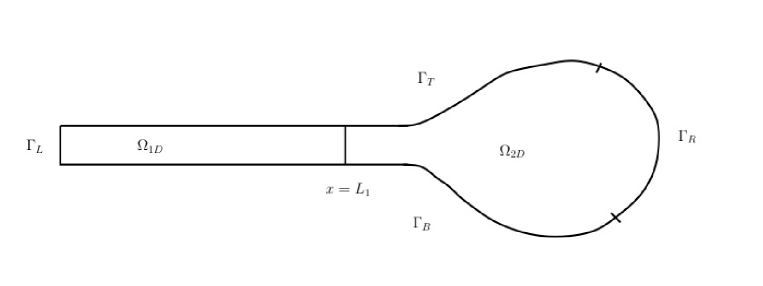
Figure 1: Typical computational domain $\Omega$, including a zone with a true 2-D behavior ($x\geq L_{1}$) together with a shallow zone where we intend to use a 1-D model ($x<L_{1}$).

Let us now consider equation (1) with the following boundary conditions (see Figure 1 for the notations):

$$-\Delta u(x,z) =F(x,z),\quad\forall(x,z)\in\Omega,$$ (2a)

$$\displaystyle\frac{\partial{u}}{\partial n}(x,z) =0,\quad\forall(x,z)\in\Gamma_{T},$$ (2b)

$$\displaystyle\frac{\partial{u}}{\partial n}(x,z)+\kappa u(x,z) =0,\quad\forall(x,z)\in\Gamma_{B},$$ (2c)

$$u(x,z) =\gamma_{1}(x,z),\quad\forall(x,z)\in\Gamma_{L},$$ (2d)

$$u(x,z) =\gamma_{2}(x,z),\quad\forall(x,z)\in\Gamma_{R}.$$ (2e)

In order to derive the 1-D model in $\Omega_{1D}=\Omega\cap\{x<L_{1}\}$, we introduce the following dimensionless variables and numbers:

$$\varepsilon=\displaystyle\frac{H}{L_{1}},$$ (3)

$$\tilde{x}=\displaystyle\frac{x}{L_{1}},\quad\tilde{z}=\displaystyle\frac{z}{H},\quad\tilde{u}(\tilde{x},\tilde{z})=\displaystyle\frac{u(x,z)}{U},\quad\tilde{F}(\tilde{x},\tilde{z})=F(x,z)\displaystyle\frac{L_{1}^{2}}{U}\mbox{ and }\tilde{\kappa}=\kappa L_{1},$$ (4)

where $L_{1}$ (resp $H$) is the characteristic length (resp height) of $\Omega_{1D}$, $\varepsilon$ is called the aspect ratio, and $U$ is a characteristic value for $u(x,z)$.
The nondimensional form of equations (2) in $\Omega_{1D}$ reads:

$$-\displaystyle\frac{\partial^{2}\tilde{u}}{\partial\tilde{x}^{2}}-\displaystyle\frac{1}{\varepsilon^{2}}\displaystyle\frac{\partial^{2}\tilde{u}}{\partial\tilde{z}^{2}}=\tilde{F}\quad\mbox{in}\quad\Omega_{1D}$$ (5a)

$$\displaystyle\frac{\partial\tilde{u}}{\partial\tilde{z}}=0\quad\mbox{on}\quad\Gamma_{T}^{1}=\Gamma_{T}\cap\partial\Omega_{1D}$$ (5b)

$$-\displaystyle\frac{1}{\varepsilon}\displaystyle\frac{\partial\tilde{u}}{\partial\tilde{z}}+\tilde{\kappa}\tilde{u}=0\quad\mbox{on}\quad\Gamma_{B}^{1}=\Gamma_{B}\cap\partial\Omega_{1D}$$ (5c)

$$\tilde{u}=\displaystyle\frac{\gamma_{1}}{U}\quad\mbox{on}\quad\Gamma_{L}^{1}=\Gamma_{L}.$$ (5d)

We assume (see [13] for the scaling of $\tilde{\kappa}$) that

$$\tilde{F}=O(1),\displaystyle\frac{\partial^{2}\tilde{u}}{\partial\tilde{x}^{2}}=O(1)\;\mbox{ and }\;\tilde{\kappa}=O(\varepsilon),$$ (6)

which is a sufficient condition to ensure that the 2-D effects are negligible in $\Omega_{1D}$. Indeed we deduce from equation (5a) that

$$\frac{\partial^{2}\tilde{u}}{\partial\tilde{z}^{2}}=O(\varepsilon^{2}).$$ (7)

By vertical integration on $(\tilde{z},1)$, and accounting for the boundary condition (5b), we find:

$$\frac{\partial\tilde{u}}{\partial\tilde{z}}=O(\varepsilon^{2})$$ (8)

and finally:

$$\tilde{u}(\tilde{x},\tilde{z})=\tilde{u}(\tilde{x},0)+O(\varepsilon^{2}).$$ (9)

Going back to original variables, we have:

$$u(x,z)=u(x,0)+O(\varepsilon^{2}),\;\forall\;(x,z)\in\Omega_{1D}.$$ (10)

We now introduce the averaging operator in the vertical direction. For any function $f$ of $z$, we set:

$$\overline{f}=\displaystyle\frac{1}{H}\int_{0}^{H}f(z)\,dz.$$ (11)

We integrate equation (9) for $z\in(0,H)$ and obtain:

$$\bar{u}(x)=u(x,0)+O(\varepsilon^{2}),\;\forall x\in[0,L].$$ (12)

We now average equation (5a) in the vertical direction, taking into account the Robin boundary condition (5c) on $\Gamma_{B}^{1}$, and find:

$$-\displaystyle\frac{\partial^{2}\bar{u}}{\partial x^{2}}+\displaystyle\frac{\kappa}{H}u(x,0)=\bar{F},$$ (13)

For every $x\in[0,L_{1}]$ we may use approximation (12) to introduce the new problem:

$$-\displaystyle\frac{\partial^{2}u_{1}}{\partial x^{2}}+\displaystyle\frac{\kappa}{H}u_{1}=\bar{F}\quad\mbox{in}\quad[0,L_{1}].$$ (14)

It will replace (1a) in $\Omega_{1D}$. As evoked in Remark 1, the reader can be easily convinced that it is particularly awkward to guess the value of $L_{1}$. Indeed one has to specify the criteria that define 2-D effects, and in practical situations we may only be able to define $L_{2}$ which is such that $\big{(}\Omega\cap\{x\geq L_{2}\}\big{)}\subset\Omega_{2D}$, or in other words $L_{2}\geq L_{1}$. In this work we consider two different situations:

• a funnel-shaped domain (see Figure 2) with a thin left part, so that we anticipate 2-D effects on the right (wide) part of the domain. In this case the definition of $L_{2}$ is based on a geometrical criterion.

• a rectangular domain (see Figure 3) with a small aspect ratio $\varepsilon=H/L$ (so that we can anticipate weak 2-D effects), but with some 2-D forcing terms occuring in the right end of the domain. In that case the definition of $L_{2}$ is based on the support of forcing terms.

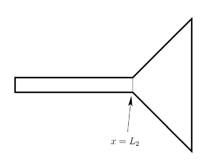
Figure 2: Funnel-shaped computational domain. The domain is shallow for $x<L_{2}$.

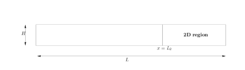
Figure 3: Rectangular computational domain $\Omega$. The domain is shallow: $H/L\ll 1$, and we assume that the forcing terms are supported in $\{x>L_{2}\}$.

At this point we have defined an upper bound $L_{2}\geq L_{1}$, but the exact value of $L_{1}$ remains unknown. From now on we choose an interface $L_{0}$ without any a priori information (other than $L_{0}<L_{2}$) and decide to consider the model reduction (17) on $\Omega_{1}=\Omega\cap\{x<L_{0}\}$, while we keep the 2-D model in $\Omega_{2}=\Omega\cap\{x>L_{0}\}$. Finally we have the two following systems

$$\mbox{1-D model: }\qquad\left\{\begin{array}[]{rcl}\displaystyle-\displaystyle\frac{\partial^{2}u_{1}}{\partial x^{2}}+\displaystyle\frac{\kappa}{H}u_{1}&=&F_{1}\mbox{ in }(0,L_{0}),\\ u_{1}(0)&=&\bar{\gamma}_{1}.\end{array}\right.$$ (17)

and

$$\mbox{2-D model: }\qquad\left\{\begin{array}[]{rcl}\displaystyle-\Delta u_{2}&=&F_{2}\mbox{ in }\Omega_{2},\\ \displaystyle\displaystyle\frac{\partial u_{2}}{\partial n}=0\mbox{ on }\Gamma^{2}_{T}&=&\Gamma_{T}\cap\partial\Omega_{2},\\ \displaystyle\displaystyle\frac{\partial u_{2}}{\partial n}+\kappa u_{2}=0\mbox{ on }\Gamma^{2}_{B}&=&\Gamma_{B}\cap\partial\Omega_{2},\\ u_{2}&=&\gamma_{2}\mbox{ on }\Gamma_{R}.\end{array}\right.$$ (22)

where $F_{1}=\overline{F}$ and $F_{2}=F_{|\Omega_{2}}$.

Two cases may occur:

• Favourable case: $L_{0}<L_{1}$, so that $\Omega_{1}\subset\Omega_{1D}$ and the following model reduction is relevant. In particular, hypothesis (6) holds so that Theorem 1 applies,

• Unfavourable case: $L_{0}\geq L_{1}$, so that $\Omega_{1}\not\subset\Omega_{1D}$ and the 1-D model will not be able to reproduce the 2-D reality (in particular, hypothesis (6) does not hold).

We now want to evaluate this model reduction in the favourable case $L_{0}<L_{1}$.

3 Coupling algorithm

Let us consider the two models (17) and (22) to be coupled respectively through the interfaces $x=L_{0}$ and $\Gamma$ as shown in Figure 4.

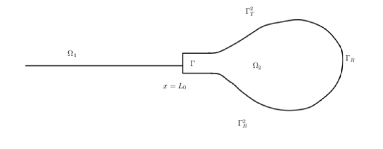
Figure 4: Computational domains for the 1-D/2-D reduced model

In coupling problems, the first difficulty lies in defining the coupling notion by itself, i.e. defining the quantities or values to be exchanged between the two models through the coupling interfaces. In our case and from a physical point of view, one may propose the following conditions, see [11], [12]:

$$u_{1}(L_{0}) =\frac{1}{H}\int_{0}^{H}u_{2}(L_{0},z)dz$$ (23a)

$$\frac{\partial u_{1}}{\partial x}(L_{0}) =\frac{1}{H}\int_{0}^{H}\frac{\partial u_{2}}{\partial x}(L_{0},z)dz$$ (23b)

which correspond to the conservation of $u$ and its flux through the interface.
Unfortunately these two constraints do not allow the well-posedness of the 2-D model and of the coupled problem. They are called defective boundary conditions in the literature, [2], [14], [12].
One should then rather apply a coupling method ensuring the following points:

• the well-posedness of the 1-D and 2-D models

• the physical constraints are satisfied

• the control of the difference between the coupled solution and the reference one (corresponding to the 2-D model over the whole domain $\Omega$). Indeed, due to the nature of the problem, the reader can be easily convinced that one does not expect to end with a solution of the 2-D model equal to the restriction of the reference one on $\Omega_{2}$.

The coupling problem with (23a) and (23b) has been studied in [11] and [12] using variational and algebraic approaches. In this section, we propose an iterative coupling method based on classical Schwarz algorithms. These iterative methods were used for the first time in the context of dimensionally heterogeneous coupling in [2] and [3] to study a nonlinear hyperbolic coupling problem.
We will prove the convergence of these algorithms given an appropriate choice of boundary conditions at $x=L_{0}$ and on $\Gamma$. Then we will study the solutions obtained after convergence and compare them to the global reference solution $u$ defined by (2). Finally we will give some results regarding the choice of the coupling interface position.

3.1 Schwarz algorithms

Let us introduce first the Schwarz algorithms in the context of dimensionally homogeneous coupling. Consider the two systems, defined on $\Omega_{1}$ and $\Omega_{2}$ shown in Figure 5:

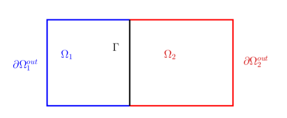
Figure 5: Computational domains for the dimensionally homogeneous coupling problem

$$\left\{\begin{array}[]{ll}\mathcal{L}_{u}u=f_{u}\;\;\;\mbox{in}\;\;\;\Omega_{1}\subset\mathbb{R}^{n}\\ B_{u}^{out}u=g_{u}\;\;\;\mbox{on}\;\;\;\partial\Omega_{1}^{out}\\ \end{array}\right.\;\;\;\mbox{and}\;\;\;\;\;\left\{\begin{array}[]{ll}\mathcal{L}_{v}v=f_{v}\;\;\;\mbox{in}\;\;\;\Omega_{2}\subset\mathbb{R}^{n}\\ B_{v}^{out}v=g_{v}\;\;\;\mbox{on}\;\;\;\partial\Omega_{2}^{out}\\ \end{array}\right.$$ (28)

The operators $\mathcal{L}_{u}$ and $\mathcal{L}_{v}$ are different. We assume that $u$ and $v$ have to satisfy the following constraints derived from the physics :

$$C_{1}u =C_{2}v$$ (29a)

$$C^{\prime}_{1}u =C^{\prime}_{2}v$$ (29b)

through the interface $\Gamma$, where $C_{1}$, $C^{\prime}_{1}$, $C_{2}$ and $C^{\prime}_{2}$ are differential operators.
To couple these two models we can implement the following iterative algorithm:
For a given $v^{0}$ and at each iteration $k\geq 0$, solve:

$$\left\{\begin{array}[]{lll}\mathcal{L}_{u}u^{k+1}&=&f_{u}\quad\mbox{in}\quad\Omega_{1}\\ B_{u}^{out}u^{k+1}&=&g_{u}\quad\mbox{on}\quad\partial\Omega_{1}^{out}\\ B_{u}u^{k+1}&=&B_{v}v^{k}\quad\mbox{on}\quad\Gamma\end{array}\right.\quad\mbox{then}\quad\left\{\begin{array}[]{lll}\mathcal{L}_{v}v^{k+1}&=&f_{v}\quad\mbox{in}\quad\Omega_{2}\\ B_{v}^{out}v^{k+1}&=&g_{v}\quad\mbox{on}\quad\partial\Omega_{2}^{out}\\ B^{\prime}_{v}v^{k+1}&=&B^{\prime}_{u}u^{k+1}\quad\mbox{on}\quad\Gamma.\end{array}\right.$$

Once convergence is achieved, the physical constraints (29a) and (29b) have to be satisfied. Then care should be taken to choose the operators $B_{u}$, $B^{\prime}_{u}$, $B_{v}$ and $B^{\prime}_{v}$ in order to ensure convergence toward the unique solution defined by (28), (29a) and (29b), see [15] and [16].
This method can be generalized to the dimensionally heterogeneous coupling case. Let assume that we have to solve the following 1-D model/2-D model coupled problem:

$$\left\{\begin{array}[]{ll}\mathcal{L}_{1}u_{1}=f_{1}\quad\mbox{in}\quad\Omega_{1}\subset\mathbb{R}\\ B_{1}^{out}u_{1}=g_{1}\quad\mbox{on}\quad\partial\Omega_{1}^{out}\\ \end{array}\right.\quad\mbox{and}\quad\left\{\begin{array}[]{ll}\mathcal{L}_{2}u_{2}=f_{2}\quad\mbox{in}\quad\Omega_{2}\subset\mathbb{R}^{2}\\ B_{2}^{out}u_{2}=g_{2}\quad\mbox{on}\quad\partial\Omega_{2}^{out}\\ \end{array}\right.$$

and we suppose that we have the following coupling constraints to satisfy at $x=L_{0}$ and on $\Gamma$:

$$C_{1}u_{1}(L_{0}) =C_{2}\left(\mathcal{R}u_{2}\right)(L_{0})$$ (30a)

$$C^{\prime}_{2}u_{2}(L_{0},z) =C^{\prime}_{1}\left(\mathcal{E}u_{1}\right)(L_{0},z)\quad\mbox{on}\quad\Gamma$$ (30b)

$\mathcal{R}u_{2}$ is a restriction of $u_{2}$ at $x=L_{0}$ and $\mathcal{E}u_{1}$ is an extension of $u_{1}(L_{0})$ all along $\Gamma$. More generally we can define the operators $\mathcal{R}$ and $\mathcal{E}$ as in [11] by:

$$\mathcal{R}:\Lambda \longrightarrow \Lambda_{0}$$

$$u_{2|\Gamma} \longmapsto \mathcal{R}u_{2|\Gamma}$$

and

$$\mathcal{E}:\Lambda_{0} \longrightarrow \Lambda$$

$$u_{1|x=L_{0}} \longmapsto \mathcal{E}u_{1|x=L_{0}}$$

The spaces $\Lambda_{0}$ et $\Lambda$ are the trace spaces on the interface $x=L_{0}$ for 1-D functions and on the interface $\Gamma$ for 2-D functions. As mentioned in [11], these two operators are not invertible.
One may thus implement the following algorithm:
For a given $u_{2}^{0}$ and at each iteration $k\geq 0$, solve:

$$\left\{\begin{array}[]{lll}\mathcal{L}_{1}u_{1}^{k+1}&=&f_{1}\quad\mbox{in}\quad\Omega_{1}\\ B_{1}^{out}u_{1}^{k+1}&=&g_{1}\quad\mbox{on}\quad\partial\Omega_{1}^{out}\\ B_{1}u_{1}^{k+1}&=&B_{2}\mathcal{R}u_{2}^{k}\quad\mbox{at}\quad x=L_{0}\end{array}\right.\quad then\quad\left\{\begin{array}[]{lll}\mathcal{L}_{2}u_{2}^{k+1}&=&f_{2}\quad\mbox{in}\quad\Omega_{2}\\ B_{2}^{out}u_{2}^{k+1}&=&g_{2}\quad\mbox{on}\quad\partial\Omega_{2}^{out}\\ B^{\prime}_{2}u_{2}^{k+1}&=&B^{\prime}_{1}\mathcal{E}u_{1}^{k+1}\quad\mbox{on}\quad\Gamma.\end{array}\right.$$

In practice, we do not have conditions such as (30a) (at $x=L_{0}$) and (30b) (for $(x,z)\mbox{ on }\Gamma$), but only conditions at $x=L_{0}$ such as (23a) and (23b). This leads us to make a choice of the operators $\mathcal{R}$, $\mathcal{E}$, $C_{1}$, $C_{2}$, $C^{\prime}_{1}$ and $C^{\prime}_{2}$.
In general the choice of the restriction operator $\mathcal{R}$ is more straightforward than the choice of the extension operator $\mathcal{E}$ one. In this study, since the 1-D model is obtained after some approximations and by averaging the 2-D model, it is reasonable to define $\mathcal{R}$ as the vertical average. On the other hand, the question of the choice of the operator $\mathcal{E}$ remains open.
In [11] and [12], authors proposed a constant extension of (23a) and (23b) along $\Gamma$, and impose the following strong coupling constraints:

$$\left\{\begin{array}[]{lll}u_{2}(L_{0},z)&=&u_{1}(L_{0})\quad\mbox{on}\quad\Gamma\\ \displaystyle\frac{\partial u_{1}}{\partial x}(L_{0})&=&\displaystyle\frac{1}{H}\int_{0}^{H}\frac{\partial u_{2}}{\partial x}(L_{0},z)dz\end{array}\right.\;\;\;\mbox{or}\;\;\;\;\;\left\{\begin{array}[]{lll}u_{1}(L_{0})&=&\displaystyle\frac{1}{H}\int_{0}^{H}u_{2}(L_{0},z)dz\\ \displaystyle\frac{\partial u_{2}}{\partial x}(L_{0},z)&=&\displaystyle\frac{\partial u_{1}}{\partial x}(L_{0})\quad\mbox{on}\quad\Gamma\end{array}\right.$$

It is a choice among many others. One may also choose a multitude of operators $C_{1}$, $C_{2}$, $C^{\prime}_{1}$ and $C^{\prime}_{2}$ ensuring the physical constraints to be satisfied.
The strategy that we adopt here is to choose, due to relations (10) and (12), a constant extension of $u_{1}$ along $\Gamma$ and then to implement a family of Schwarz algorithms with appropriate boundary conditions at $x=L_{0}$ and on $\Gamma$. In this case Schwarz coupling algorithm reads:
For a given $u_{2}^{0}$ and at each iteration $k\geq 0$, solve :

$$\left\{\begin{array}[]{lllll}\displaystyle-\displaystyle\frac{\partial^{2}{u_{1}^{k+1}}}{\partial x^{2}}+\frac{\kappa}{H}u_{1}^{k+1}=F_{1}\quad\mbox{in}\quad(0,L_{0})\\ \\ u_{1}^{k+1}(0)=\bar{\gamma}_{1}\\ \\ \displaystyle B_{1}u_{1}^{k+1}(L_{0})=B_{1}\bar{u}_{2}^{k}\end{array}\right.$$ (36)

and then solve

$$\left\{\begin{array}[]{lllllll}-\Delta u_{2}^{k+1}=F_{2}\quad\mbox{in}\quad\Omega_{2}\\ \\ \displaystyle\displaystyle\frac{\partial{u_{2}^{k+1}}}{\partial n}=0\quad\mbox{on}\quad\Gamma_{T}^{2}\\ \\ \displaystyle\displaystyle\frac{\partial{u_{2}^{k+1}}}{\partial n}+\kappa u_{2}^{k+1}=0\quad\mbox{on}\quad\Gamma_{B}^{2}\\ \\ u_{2}^{k+1}=\gamma_{2}\quad\mbox{on}\quad\Gamma_{R}\\ \\ \displaystyle B_{2}u_{2}^{k+1}=B_{2}u_{1}^{k+1}\quad\mbox{on}\quad\Gamma\end{array}\right.$$ (46)

The linear operators $B_{1}$ and $B_{2}$ will be defined such that the points (i), (ii) and (iii) (see introduction of Section 3) are satisfied and such that the algorithm converges.
We will first study the convergence of the coupling algorithm. Subsequently we move on the point (iii).
To ensure the convergence of Schwarz algorithms in the case of classical domain decomposition without overlapping, it is proposed in [17] to use Robin operators. We will extend the use of these operators to our coupling problem. We define the operators $B_{1}$ and $B_{2}$ for a given $\lambda>0$ as follows:

$$B_{1}=\frac{\partial}{\partial n_{1}}+\lambda Id$$ (47)

and

$$B_{2}=\displaystyle\frac{\partial{}}{\partial n_{2}}+\lambda Id$$ (48)

where $n_{1}$ and $n_{2}$ are the outward unit normal to the 1-D and 2-D domains respectively. We note that the operators $B_{1}$ and $B_{2}$ ensure the well-posedness of the problem at each iteration. Let us study the convergence of Schwarz algorithm with this family of operators.

3.2 Algorithm convergence

Proposition 1.

For each $\lambda>0$, the $(u_{1}^{k},u_{2}^{k})$ Schwarz algorithm converges in $H^{1}(\Omega_{1})\times H^{1}(\Omega_{2})$ to $(u_{1}^{\lambda},u_{2}^{\lambda})$ that satisfies the physical constraints (23a), (23b).

Proof:
Let define the differences between two successive iterations:

$$e_{1}^{k+1}(x)=u_{1}^{k+1}(x)-u_{1}^{k}(x),\quad\forall x\in(0,L_{0})$$

and

$$e_{2}^{k+1}(x,z)=u_{2}^{k+1}(x,z)-u_{2}^{k}(x,z),\quad\forall(x,z)\in\Omega_{2}$$

These functions satisfy the following systems:

$$\left\{\begin{array}[]{lllll}\displaystyle-\displaystyle\frac{\partial^{2}{e_{1}^{k+1}}}{\partial x^{2}}+\frac{\kappa}{H}e_{1}^{k+1}=0\quad\mbox{in}\quad(0,L_{0})\\ \\ e_{1}^{k+1}(0)=0\\ \\ \displaystyle\frac{\partial e_{1}^{k+1}}{\partial x}(L_{0})+\lambda e_{1}^{k+1}(L_{0})=\frac{\partial\bar{e}_{2}^{k}}{\partial x}(L_{0})+\lambda\bar{e}_{2}^{k}(L_{0})\end{array}\right.$$ (54)

and

$$\left\{\begin{array}[]{lllllll}-\Delta e_{2}^{k+1}=0\quad\mbox{in}\quad\Omega_{2}\\ \\ \displaystyle\displaystyle\frac{\partial{e_{2}^{k+1}}}{\partial n}=0\quad\mbox{on}\quad\Gamma_{T}^{2}\\ \\ \displaystyle\displaystyle\frac{\partial{e_{2}^{k+1}}}{\partial n}+\kappa e_{2}^{k+1}=0\quad\mbox{on}\quad\Gamma_{B}^{2}\\ \\ e_{2}^{k+1}=0\quad\mbox{on}\quad\Gamma_{R}\\ \\ \displaystyle-\frac{\partial e_{2}^{k+1}}{\partial x}(L_{0},z)+\lambda e_{2}^{k+1}(L_{0},z)=-\frac{\partial e_{1}^{k+1}}{\partial x}(L_{0})+\lambda e_{1}^{k+1}(L_{0})\quad\mbox{on}\quad\Gamma.\end{array}\right.$$ (64)

The first two equations of (54) lead to:

$$e_{1}^{k+1}(x)=\alpha_{k+1}\sinh(ax),\;\;\;\forall x\in(0,L_{0})$$ (65)

where $\alpha_{k+1}\in\mathbb{R}$ and $\displaystyle a=\sqrt{\frac{\kappa}{H}}$.
If we take the vertical average of the boundary condition on $\Gamma$ in (64), and due to the boundary condition at $x=L_{0}$, we obtain :

$$\left\{\begin{array}[]{ccc}\displaystyle-\frac{\partial\bar{e}_{2}^{k+1}}{\partial x}(L_{0})+\lambda\bar{e}_{2}^{k+1}(L_{0})&=&\displaystyle-\frac{\partial e_{1}^{k+1}}{\partial x}(L_{0})+\lambda e_{1}^{k+1}(L_{0})\\ \\ \displaystyle\frac{\partial\bar{e}_{2}^{k+1}}{\partial x}(L_{0})+\lambda\bar{e}_{2}^{k+1}(L_{0})&=&\displaystyle\frac{\partial e_{1}^{k+2}}{\partial x}(L_{0})+\lambda e_{1}^{k+2}(L_{0}).\end{array}\right.$$

This implies:

$$\bar{e}_{2}^{k+1}(L_{0}) = \frac{1}{2\lambda}\left(A\alpha_{k+2}+B\alpha_{k+1}\right)$$ (66)

and

$$\displaystyle\frac{\partial{\bar{e}_{2}^{k+1}}}{\partial x}(L_{0})=\frac{1}{2}\left(A\alpha_{k+2}-B\alpha_{k+1}\right)$$ (67)

where $A=a\cosh(aL_{0})+\lambda\sinh(aL_{0})$ and $B=-a\cosh(aL_{0})+\lambda\sinh(aL_{0})$.
Now by multiplying the first equation of (64) by $e_{2}^{k+1}$ and by integrating in $\Omega_{2}$, we obtain:

$$\int_{\Omega_{2}}|\nabla e_{2}^{k+1}|^{2}dxdz-\int_{\partial\Omega_{2}}\frac{\partial e_{2}^{k+1}}{\partial n}e_{2}^{k+1}d\sigma=0$$

then using the boundary conditions on $\Gamma_{T}^{2}$ and $\Gamma_{R}$, we obtain:

$$\int_{\Omega_{2}}|\nabla e_{2}^{k+1}|^{2}dxdz+\int_{\Gamma_{B}^{2}}\kappa|e_{2}^{k+1}|^{2}dx = -\int_{\Gamma}\frac{\partial e_{2}^{k+1}}{\partial x}(L_{0},z)e_{2}^{k+1}(L_{0},z)dz.$$ (68)

We replace $\displaystyle\frac{\partial e_{2}^{k+1}}{\partial x}(L_{0},z)$ in (68) by its value obtained by using Robin boundary condition on $\Gamma$:

$$\int_{\Omega_{2}}|\nabla e_{2}^{k+1}|^{2}dxdz+\int_{\Gamma_{B}^{2}}\kappa|e_{2}^{k+1}|^{2}dx = \int_{\Gamma}\left(-\frac{\partial e_{1}^{k+1}}{\partial x}(L_{0})+\lambda e_{1}^{k+1}(L_{0})-\lambda e_{2}^{k+1}(L_{0},z)\right)e_{2}^{k+1}(L_{0},z)dz$$ (69)

$$= B\alpha_{k+1}H\bar{e}_{2}^{k+1}(L_{0})-\lambda\int_{0}^{H}|e_{2}^{k+1}|^{2}(L_{0},z)dz$$

$$= \frac{B\alpha_{k+1}H}{2\lambda}\left(A\alpha_{k+2}+B\alpha_{k+1}\right)-\lambda\int_{0}^{H}|e_{2}^{k+1}|^{2}(L_{0},z)dz.$$

We now replace $e_{2}^{k+1}(L_{0},z)$ in (68) using the same Robin boundary condition:

$$\int_{\Omega_{2}}|\nabla e_{2}^{k+1}|^{2}dxdz+\int_{\Gamma_{B}^{2}}\kappa|e_{2}^{k+1}|^{2}d\sigma = -\int_{\Gamma}\frac{1}{\lambda}\left(-\frac{\partial e_{1}^{k+1}}{\partial x}(L_{0})+\lambda e_{1}^{k+1}(L_{0})\right)\frac{\partial e_{2}^{k+1}}{\partial x}(L_{0},z)dz$$

$$-\frac{1}{\lambda}\int_{0}^{H}\left|\frac{\partial e_{2}^{k+1}}{\partial x}(L_{0},z)\right|^{2}dz$$

$$= -\frac{B\alpha_{k+1}H}{\lambda}\frac{\partial\bar{e}_{2}^{k+1}}{\partial x}(L_{0})-\frac{1}{\lambda}\int_{0}^{H}\left|\frac{\partial e_{2}^{k+1}}{\partial x}(L_{0},z)\right|^{2}dz$$

$$= -\frac{B\alpha_{k+1}H}{2\lambda}\left(A\alpha_{k+2}-B\alpha_{k+1}\right)-\frac{1}{\lambda}\int_{0}^{H}\left|\frac{\partial e_{2}^{k+1}}{\partial x}(L_{0},z)\right|^{2}dz.$$

Due to the fact that $\lambda>0$, we deduce that:

$$\frac{B\alpha_{k+1}H}{2\lambda}\left(A\alpha_{k+2}+B\alpha_{k+1}\right)\geq 0$$

and

$$-\frac{B\alpha_{k+1}H}{2\lambda}\left(A\alpha_{k+2}-B\alpha_{k+1}\right)\geq 0.$$

Thus:

$$A^{2}\alpha_{k+2}^{2}-B^{2}\alpha_{k+1}^{2}\leq 0.$$

Then we obtain:

$$\frac{\alpha_{k+2}^{2}}{\alpha_{k+1}^{2}}\leq\frac{B^{2}}{A^{2}}=\left|\frac{-a\cosh(aL_{0})+\lambda\sinh(aL_{0})}{a\cosh(aL_{0})+\lambda\sinh(aL_{0})}\right|^{2}<1$$

and finally

$$\left|\frac{\alpha_{k+2}}{\alpha_{k+1}}\right|<\left|\frac{B}{A}\right|<1.$$ (70)

So that the sequence $(\alpha_{k})_{k\in\mathbb{N}}$ converge to zero.
Let us now remark that for all $k\geq 0$, $n\geq 0$, we have:

$$u_{1}^{k+n}-u_{1}^{k} = \sum_{p=0}^{n-1}e_{1}^{k+p+1}$$

and

$$\frac{\partial\left(u_{1}^{k+n}-u_{1}^{k}\right)}{\partial x} = \sum_{p=0}^{n-1}\frac{\partial e_{1}^{k+p+1}}{\partial x}$$

Using the relation (65) and the fact that the sequence $(\alpha_{k})_{k\in\mathbb{N}}$ converges, we can prove that $(u_{1}^{k})_{k\in\mathbb{N}}$ and $\displaystyle(\frac{\partial u_{1}^{k}}{\partial x})_{k\in\mathbb{N}}$ are Cauchy sequences in $L^{2}(\Omega_{1})$. So that $(u_{1}^{k})_{k\in\mathbb{N}}$ is a Cauchy sequence in $H^{1}(\Omega_{1})$.
In the same way we observe that for all $k\geq 0$, $n\geq 0$, we have:

$$\nabla(u_{2}^{k+n}-u_{2}^{k}) = \sum_{p=0}^{n-1}\nabla e_{2}^{k+p+1}$$

Using (69), we deduce that:

$$\int_{\Omega_{2}}|\nabla e_{2}^{k+1}|^{2}dxdz\leq\frac{B\alpha_{k+1}H}{2\lambda}\left(A\alpha_{k+2}+B\alpha_{k+1}\right)$$

and then we can prove that $(\nabla e_{2}^{k})_{k\in\mathbb{N}}$ is a Cauchy sequence in $L^{2}(\Omega_{2})$ and due to the Poincaré inequality we have also $(u_{2}^{k})_{k\in\mathbb{N}}$ is a Cauchy sequence in $L^{2}(\Omega_{2})$. So that $(u_{2}^{k})_{k\in\mathbb{N}}$ is a Cauchy sequence in $H^{1}(\Omega_{2})$.
To conclude we have prove that $(u_{1}^{k},u_{2}^{k})$ Schwarz algorithm converges in $H^{1}(\Omega_{1})\times H^{1}(\Omega_{2})$. Moreover, at convergence the limit $(u_{1}^{\lambda},u_{2}^{\lambda})$ verifies $B_{2}u_{2}^{\lambda}=B_{2}u_{1}^{\lambda}$ and $B_{1}u_{1}^{\lambda}=B_{1}\bar{u}_{2}^{\lambda}$. Taking the vertical average on $\Gamma$ gives two linear combinations of the constraints (23a), (23b).$\Box$

Remark 2.

• The Schwarz algorithms converge for all $\lambda$ positive, but we remark that for $\displaystyle\lambda=a\coth(aL_{0})$, we have exact convergence in two iterations. Indeed we have in this case:

  $$-\frac{\partial e_{1}^{k+1}}{\partial x}+a\coth(aL_{0})e_{1}^{k+1}=0\;\;\;\forall k\geq 0,$$

  and then:

  $$B_{2}e_{2}^{k+1}=-\frac{\partial e_{2}^{k+1}}{\partial x}+a\coth(aL_{0})e_{2}^{k+1}=-\frac{\partial e_{1}^{k+1}}{\partial x}+a\coth(aL_{0})e_{1}^{k+1}=0\;\;\;\forall k\geq 0,$$

  The operator $\displaystyle\displaystyle\frac{\partial{}}{\partial n_{1}}+a\coth(aL_{0})Id$ corresponds to the absorbing operator of the 1-D model.
  We denote by $\lambda_{opt}$ this value of $\lambda$, see for example [18].

• If we take $\lambda_{1}\neq\lambda_{2}$, we have a priori $(u_{1}^{\lambda_{1}},u_{2}^{\lambda_{1}})\neq(u_{1}^{\lambda_{2}},u_{2}^{\lambda_{2}})$. This is in accordance with the ill-posedness of coupling problem defined by (17), (22), (23a) and (23b).

For the sake of clarity we will denote $(u_{1},u_{2})$ the limit of Schwarz algorithm instead of $(u_{1}^{\lambda},u_{2}^{\lambda})$.

3.3 Control of the difference between the coupled solution and the global reference solution

Unlike the case of domain decomposition, at convergence of Schwarz algorithm, we have $u_{2}\neq u|_{\Omega_{2}}$ due to the model reduction. But as mentioned above, we have chosen the family of Robin operators in order to get some control of the difference between $u_{2}$ and $u|_{\Omega_{2}}$. In fact we have the following result:

Theorem 1.

for each $\lambda>0$, let $(u_{1}^{\lambda},u_{2}^{\lambda})$ denotes the limit of the Schwarz algorithm. If $L_{0}<L_{1}$ then there exists $M(\lambda)>0$ such that:

$$\|u_{|\Omega_{2}}-u_{2}\|_{H^{1}(\Omega_{2})}\leq M(\lambda)\varepsilon\sqrt{1+\delta^{2}}$$ (71)

where $\displaystyle\delta=\frac{L_{1}}{L_{1}-L_{0}}$.

Proof
The function $u|_{\Omega_{2}}-u_{2}$ is the solution of the system:

$$\left\{\begin{array}[]{lllllllll}\displaystyle-\Delta(u-u_{2})=0\quad\mbox{in}\quad\Omega_{2}\\ \\ \displaystyle\frac{\partial(u-u_{2})}{\partial n}=0\quad\mbox{on}\quad\Gamma^{2}_{T}\\ \\ \displaystyle\frac{\partial(u-u_{2})}{\partial n}+\kappa(u-u_{2})=0\quad\mbox{on}\quad\Gamma^{2}_{B}\\ \\ u-u_{2}=0\quad\mbox{on}\quad\Gamma_{R}.\end{array}\right.$$

By multiplying the first equation by $u-u_{2}$ and using the boundary conditions on $\Gamma_{T}^{2}\cup\Gamma_{B}^{2}\cup\Gamma_{R}$, we obtain:

$$\int_{\Omega_{2}}|\nabla\left(u-u_{2}\right)|^{2}dxdz+\int_{\Gamma_{B}^{2}}\kappa|u-u_{2}|^{2}dx-\int_{\Gamma}\frac{\partial(u-u_{2})}{\partial n}\left(u-u_{2}\right)dz=0. *$$ ()

The integral term on $\Gamma$ is reformulated using the boundary condition $\displaystyle-\frac{\partial u_{2}}{\partial x}+\lambda u_{2}=-\frac{\partial u_{1}}{\partial x}+\lambda u_{1}$ satisfied by the limit $u_{2}$:

$$\int_{\Gamma}\frac{\partial(u-u_{2})}{\partial n}\left(u-u_{2}\right)dz = -\int_{0}^{H}\frac{\partial(u-u_{2})}{\partial x}(L_{0},z)\left(u-u_{2}\right)(L_{0},z)dz$$

$$= -\int_{0}^{H}\frac{\partial u}{\partial x}(L_{0},z)\left(u-u_{2}\right)(L_{0},z)dz$$

$$-\int_{0}^{H}\left(-\frac{\partial u_{1}}{\partial x}(L_{0})+\lambda u_{1}(L_{0})-\lambda u_{2}(L_{0},z)\right)\left(u-u_{2}\right)(L_{0},z)dz$$

$$= \int_{0}^{H}\left(-\frac{\partial u}{\partial x}(L_{0},z)+\lambda u(L_{0},z)\right)\left(u-u_{2}\right)(L_{0},z)dz$$

$$-\int_{0}^{H}\left(-\frac{\partial u_{1}}{\partial x}(L_{0})+\lambda u_{1}(L_{0})\right)\left(u-u_{2}\right)(L_{0},z)dz$$

$$-\lambda\int_{0}^{H}\left(u-u_{2}\right)^{2}(L_{0},z)dz.$$

$\bullet$ The first term reads:

$$\int_{0}^{H}\left(-\frac{\partial u}{\partial x}+\lambda u\right)(L_{0},z)\left(u-u_{2}\right)(L_{0},z)dz = \int_{0}^{H}\left(-\frac{\partial u}{\partial x}+\lambda u\right)(L_{0},z)\left(u(L_{0},z)-\bar{u}(L_{0})\right)dz$$

$$+\int_{0}^{H}\left(-\frac{\partial u}{\partial x}+\lambda u\right)(L_{0},z)\left(\bar{u}(L_{0})-u_{1}(L_{0})\right)dz$$

$$+\int_{0}^{H}\left(-\frac{\partial u}{\partial x}+\lambda u\right)(L_{0},z)\left(u_{1}(L_{0})-u_{2}(L_{0},z)\right)dz.$$

Due to the relations (10) and (12) and to the fact that $\displaystyle-\frac{\partial u}{\partial x}(L_{0},z)+\lambda u(L_{0},z)=O(1)$, we deduce:

$$\int_{0}^{H}\left(-\frac{\partial u}{\partial x}+\lambda u\right)(L_{0},z)\left(u(L_{0},z)-\bar{u}(L_{0})\right)dz=O(\varepsilon^{2})$$

In the same way, if we assume that $L_{0}<L_{1}$, so that 2-D effects are insignificant in $\Omega_{1}\cap{\{L_{0}\leq x\leq L_{1}\}}$, and applying a similar asymptotic analysis as in the first section to the 2-D model defined in $\Omega_{2}$, we can deduce that:

$$u_{2}(L_{0},z) = \bar{u}_{2}(L_{0})+O(\delta^{2}\varepsilon^{2})$$ (73)

$$= u_{1}(L_{0})+O(\delta^{2}\varepsilon^{2}),\quad\forall z\in[0,H]$$

So that:

$$\int_{0}^{H}\left(-\frac{\partial u}{\partial x}+\lambda u\right)(L_{0},z)\left(u_{1}(L_{0})-u_{2}(L_{0},z)\right)dz=O(\delta^{2}\varepsilon^{2})$$

Finally:

$$\int_{0}^{H}\left(-\frac{\partial u}{\partial x}+\lambda u\right)(L_{0},z)\left(\bar{u}(L_{0})-u_{1}(L_{0})\right)dz=H\left(-\frac{\partial\bar{u}}{\partial x}+\lambda\bar{u}\right)(L_{0})\left(\bar{u}(L_{0})-u_{1}(L_{0})\right)$$ (74)

$\bullet$ Since $u_{1}(L_{0})=\overline{u}_{2}(L_{0})$, the second term reads:

$$-\int_{0}^{H}\left(-\frac{\partial u_{1}}{\partial x}(L_{0})+\lambda u_{1}(L_{0})\right)\left(u-u_{2}\right)(L_{0},z)dz =-H\left(-\frac{\partial(u_{1}-\bar{u})}{\partial x}+\lambda(u_{1}-\bar{u})\right)(L_{0})\left(\bar{u}-u_{1}\right)(L_{0})$$

$$-H\left(-\frac{\partial\bar{u}}{\partial x}+\lambda\bar{u}\right)(L_{0})\left(\bar{u}-u_{1}\right)(L_{0}) **$$ ()

We reformulate the first term of the right. Note that the function $u_{1}-\bar{u}$ satisfies the equation:

$$-\frac{\partial^{2}(u_{1}-\bar{u})}{\partial x^{2}}(x)+a^{2}(u_{1}-\bar{u})(x)=a^{2}(\bar{u}(x)-u(x,0)),\;\;\;\forall x\in(0,L_{0})$$

So that by multiplying this equation by $u_{1}-\bar{u}$, after integration on $(0,L_{0})$ and use of the boundary condition $u_{1}(0)=\overline{u}(0)$, we obtain:

$$\int_{0}^{L_{0}}\left(\frac{\partial(u_{1}-\bar{u})}{\partial x}\right)^{2}(x)dx+a^{2}\int_{0}^{L_{0}}\left(u_{1}-\bar{u}\right)^{2}(x)dx-\frac{\partial(u_{1}-\bar{u})}{\partial x}(L_{0})(u_{1}-\bar{u})(L_{0})=$$

$$\int_{0}^{L_{0}}a^{2}(\bar{u}(x)-u(x,0))(u_{1}(x)-\bar{u})(x)dx$$

thus:

$$-\frac{\partial(u_{1}-\bar{u})}{\partial x}(L_{0})(u_{1}-\bar{u})(L_{0})=\int_{0}^{L_{0}}a^{2}(\bar{u}(x)-u(x,0))(u_{1}(x)-\bar{u}(x))dx-\mathcal{A}_{1}(u_{1}-\bar{u},u_{1}-\bar{u})$$

where $\displaystyle\mathcal{A}_{1}(u_{1}-\bar{u},u_{1}-\bar{u})=\int_{0}^{L_{0}}\left(\frac{\partial(u_{1}-\bar{u})}{\partial x}\right)^{2}(x)dx+a^{2}\int_{0}^{L_{0}}\left(u_{1}-\bar{u}\right)^{2}(x)dx$.
And then (3.3) becomes:

$$-\int_{0}^{H}\left(-\frac{\partial u_{1}}{\partial x}(L_{0})+\lambda u_{1}(L_{0})\right)\left(u-u_{2}\right)dz = H\int_{0}^{L_{0}}a^{2}(\bar{u}(x)-u(x,0))(u_{1}(x)-\bar{u}(x))dx$$ (75)

$$-H\mathcal{A}_{1}(u_{1}-\bar{u},u_{1}-\bar{u})+\lambda H\left(\bar{u}-u_{1}\right)^{2}(L_{0})$$

$$-H\left(-\frac{\partial\bar{u}}{\partial x}+\lambda\bar{u}\right)(L_{0})\left(\bar{u}-u_{1}\right)(L_{0})$$

$\bullet$ To recap, the boundary term on $\Gamma$ in ($*$ ‣ 3.3) becomes:

$$\int_{\Gamma}\frac{\partial(u-u_{2})}{\partial n}\left(u-u_{2}\right)dz = O(\varepsilon^{2})+O(\delta^{2}\varepsilon^{2})+H\int_{0}^{L_{0}}a^{2}(\bar{u}(x)-u(x,0))(u_{1}(x)-\bar{u})dx$$

$$-H\mathcal{A}(u_{1}-\bar{u},u_{1}-\bar{u})+\lambda H\left(\bar{u}-u_{1}\right)^{2}(L_{0})$$

$$-\lambda\int_{0}^{H}\left(u-u_{2}\right)^{2}dz$$

We first observe that:

$$\int_{0}^{L_{0}}a^{2}(\bar{u}(x)-u(x,0))(u_{1}(x)-\bar{u}(x))dx\leq\frac{a^{2}}{2}\int_{0}^{L_{0}}(\bar{u}(x)-u(x,0))^{2}dx+\frac{a^{2}}{2}\int_{0}^{L_{0}}(u_{1}(x)-\bar{u}(x))^{2}dx.$$

It follows that:

$$\int_{\Gamma}\frac{\partial(u-u_{2})}{\partial n}\left(u-u_{2}\right)dz \leq C(1+\delta^{2})\varepsilon^{2})+H\frac{a^{2}}{2}\int_{0}^{L_{0}}(\bar{u}(x)-u(x,0))^{2}dx$$

$$-H\mathcal{A}_{1}(u_{1}-\bar{u},u_{1}-\bar{u})+H\frac{a^{2}}{2}\int_{0}^{L_{0}}(u_{1}(x)-\bar{u}(x))^{2}dx$$

$$+\lambda H\left(\bar{u}-u_{1}\right)^{2}(L_{0})-\lambda\int_{0}^{H}\left(u-u_{2}\right)^{2}(L_{0},z)dz$$

where $C$ is a positive constant.
Then we have:

$$-\mathcal{A}_{1}(u_{1}-\bar{u},u_{1}-\bar{u})+\frac{a^{2}}{2}\int_{0}^{L_{0}}(u_{1}(x)-\bar{u}(x))^{2}dx\leq 0$$

and finally, using the definition of $\overline{u}(L_{0})$ and the relation $u_{1}(L_{0})=\overline{u}_{2}(L_{0})$, we obtain:

$$\lambda H\left(\bar{u}-u_{1}\right)^{2}(L_{0})-\lambda\int_{0}^{H}\left(u-u_{2}\right)^{2}dz = \lambda H\left(\frac{1}{H}\int_{0}^{H}(u-u_{2})dz\right)^{2}-\lambda\int_{0}^{H}\left(u-u_{2}\right)^{2}dz$$

$$= \lambda\frac{1}{H}\left(\int_{0}^{H}(u-u_{2})dz\right)^{2}-\lambda\int_{0}^{H}\left(u-u_{2}\right)^{2}dz$$

$$\leq \lambda\frac{1}{H}\left(\int_{0}^{H}1dz\right)\left(\int_{0}^{H}(u-u_{2})^{2}dz\right)-\lambda\int_{0}^{H}\left(u-u_{2}\right)^{2}dz$$

$$\leq 0.$$

We now come back to ($*$ ‣ 3.3), which gives:

$$\int_{\Omega_{2}}|\nabla\left(u-u_{2}\right)|^{2}dxdz+\int_{\Gamma_{B}^{2}}\kappa|u-u_{2}|^{2}dx \leq M(1+\delta^{2})\varepsilon^{2}$$

and thus:

$$\int_{\Omega_{2}}|\nabla\left(u-u_{2}\right)|^{2}dxdz\leq M(1+\delta^{2})\varepsilon^{2}$$

Where $M$ denotes a positive constant.
Finally, due to the fact that $u-u_{2}=0$ on $\Gamma_{R}$, and by using Poincaré inequality we can deduce the inequality (71).$\Box$

Remark 3.

• This proposition fails if we choose the interface position in a zone where 2-D effects are significant. In this case relation (73) is no more available.

• The right term of (71) is also an upper bound of $\|u_{2}^{\lambda_{1}}-u_{2}^{\lambda_{2}}\|_{H^{1}(\Omega_{2})}$ for all $\lambda_{1}$ and $\lambda_{2}$ positive.

4 Numerical results

The test cases presented in this section illustrate the coupling method of 1-D and 2-D elliptic equations based on Schwarz algorithm. All the computations have been done using the software package Freefem++ [19], with a $P_{2}$ finite element discretization.
In the first part of this section, the two test cases will be described in details. In the second and third parts, we will focus on one hand on the Scharwz algorithm convergence and on the other hand on the comparison of the coupled solution with the reference solution in order to enlight the theoretical results obtained in the previous paragraphs.

4.1 Description of the test cases

4.1.1 Test #1:

The first test case is concerned with the solution of the 2-D problem (2) where the domain is a rectangle $\Omega=[0,L]\times[0,H]$ which is assumed to be uniformly shallow: $H\ll L$. Let us consider that the right-hand side term $F(x,z)$ of the full 2-D problem is $\displaystyle F(x,z)=m\exp(-(x-x^{*})^{2})\sin(\frac{2\pi z}{H})$, where $x^{*}<L$.
The global reference solution $u$ is displayed in Figure 6.

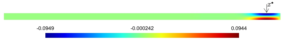
Figure 6: 2-D reference solution for the first test case where $L=20$, $x^{*}=19$, $H=0.5$ and $\kappa=0.001$.

We notice that the 2-D effects are due to the particular form of the forcing term $F$ and are located around $x^{*}$.

Now let us define the coupled model.
The interface is located at $x=L_{0}<x^{*}$ as shown in Figure 7. In the part of the domain $\Omega_{1}=[0,L_{0}]\times[0,H]$, we assume a priori that the 2-D effects are negligible and consequently we replace the full 2-D equations by the 1-D model (see (17)).

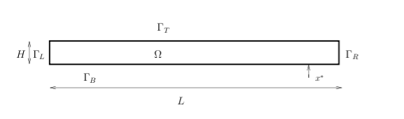
(a) Computational domain for the 2-D reference model

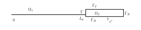
(b) Computational domain for the 1-D/2-D reduced model

Figure 7: Computational domains for both the reference and reduced models in test case #1. For the reduced model (b), the 1-D/2-D interface $\Gamma$ is located in $x=L_{0}$.

4.1.2 Test #2:

In this second test case, the 2-D effects are due to the funnel-shaped geometry of the domain (see Figure 8a), and the forcing term is constant ($=1$).

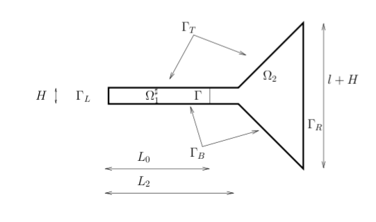
(a) Computational domain for the 2-D reference model

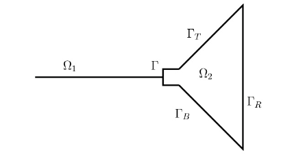
(b) Computational domain for the 1-D/2-D reduced model

Figure 8: Computational domains for both the reference and reduced models in test case #2. For the reduced model (b), the 1-D/2-D interface $\Gamma$ is located in $x=L_{0}$.

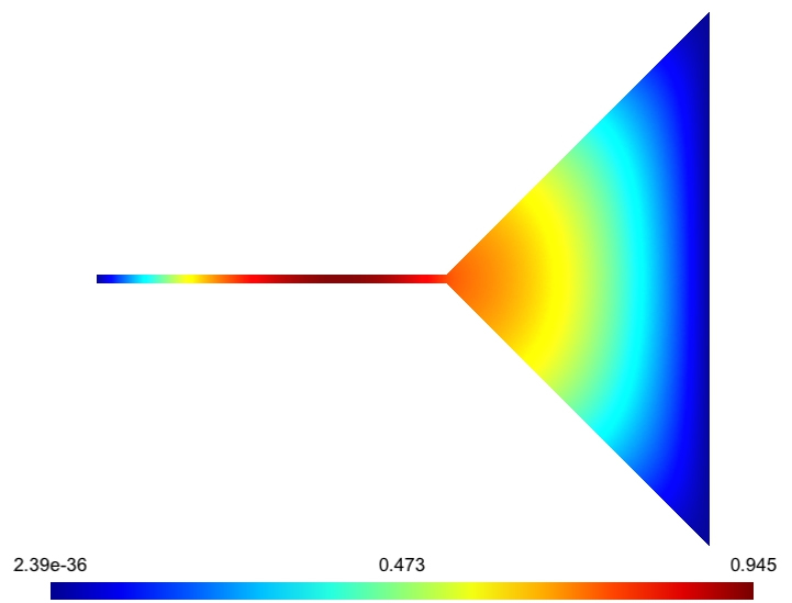
Figure 9: 2-D reference solution for the second test case where $L=2$, $H=0.05$, $l=3$ and $\kappa=0.001$

The reference solution in the whole domain is displayed in Figure 9.
The coupled model is defined by splitting the domain in two parts. The interface $\Gamma$ is located at $x=L_{0}$, $0<L_{0}<L_{2}$ as shown in Figure 8.

4.2 Convergence of the Schwarz algorithm

In this section we provide numerical results to assess the theoretical results of §3. We are interested in illustrating the optimal convergence of Schwarz algorithm for the parameter $\lambda=\lambda_{opt}$. Figure 10a shows the difference between the iterates of the Schwarz algorithm in $L^{\infty}$ norm for the two test cases.
As demonstrated in §3, the Schwarz algorithm converges in two iterations for the optimal parametrer $\lambda=\lambda_{opt}$. It is important to notice that this result is independent of the interface location.

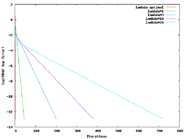
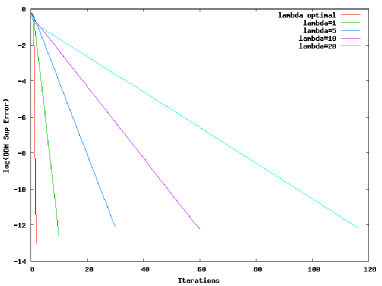
(a)

Figure 10: Convergence of Schwarz algorithm with various values of $\lambda$. Left: test case #1 with $L=20$, $L_{0}=16$, $H=0.5$ and $\kappa=0.001$. Right: test case #2 with $L=2$, $L_{0}=1.5$, $H=0.05$, $l=3$ and $\kappa=0.001$.

4.3 Difference between the coupled solution and the full 2-D solution

One important point in the analysis of the accuracy of the coupling procedure is the comparison of the coupled solution with the reference solution as a function of the interface location $x=L_{0}$. Contrarily to the classical domain decomposition problems, here there is a difference between the (converged) coupled solution and the full 2-D solution; this difference is due to the model reduction that is performed in the 1-D part of the domain. This difference depends on the location chosen to discriminate between 1-D and 2-D regions. Figures 11a and 11b left show the $H^{1}$ error between coupled and reference solutions as a function of the interface location for the two test cases. Figures 11a and 11b right show the $H^{1}$ error in $\Omega_{2}$ between coupled and reference solutions as a function of $\displaystyle\varepsilon=\frac{H}{L}$ for the two test cases.

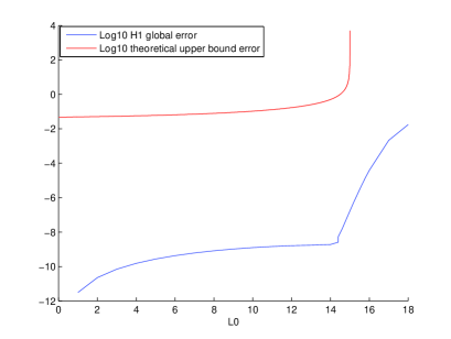
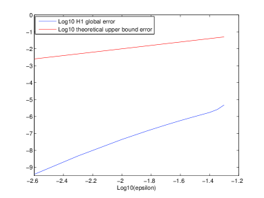
(a) Test case # 1: (left): $L=20$, $H=0.5$ and $\kappa=0.001$. (right): $L=20$, $L_{0}=14$ and $\kappa=0.01$.

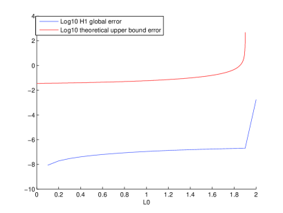
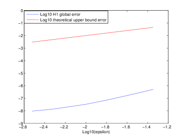
(b) Test case # 2: (left): $L=2$, $H=0.05$ and $\kappa=0.001$. (right): $L=2$, $L_{0}=1.5$ and $\kappa=0.001$.

Figure 11: Relative error as a function of $L_{0}$ (left) and $\varepsilon$ (right) between the coupled solution and the 2-D reference solution in test case #1 (top) and #2 (bottom). In the left column, the red curves correspond (for both test cases) to the RHS of estimate (71).

It is interesting to notice that for both test cases there is a discontinuity in the curve representing the error as a function of $L_{0}$ (see Figure 11, left column). This discontinuity occurs both for the numerical difference between $u_{2}$ and $u_{\Omega_{2}}$ (black curve), and the theoretical curve (in red) corresponding to the right-hand-side of estimate (71). Indeed, if $L_{0}$ is greater than a certain threshold, the error grows very rapidly (and $\delta\longrightarrow\infty$ in estimate (71)). This could be an indication of the real (a priori unknown) value of $L_{1}$ (see discussion at the end of Section 2 above).

5 Conclusion

In this paper we studied a linear boundary valued problem set in a 2-D domain, and assume that the solution may be approximated by a 1-D function in some part of the computational domain. We thus derive a reduced model that consists coupling a 1-D model (wherever we think it is legitimate) together with the original 2-D system (everywhere else).
The model reduction is performed thanks to a small aspect ratio hypothesis, with an integration in the shallow direction (we mimic the derivation of the shallow water equations). After this derivation we introduce an iterative method that couples the 1-D and 2-D systems and we prove some convergence results. One original aspect of this work is the particular attention that is paid to the location of the 1-D/2-D interface. These theoretical results are illustrated with numerical simulations that underline the importance of the interface position, but also the way 1-D and 2-D models are coupled (boundary conditions at this interface). All these aspects, that have been studied here with a linear model, will be considered in a forthcoming study of dimensionally heterogeneous modelling in fluid dynamics.

References

• [1] J. F. Gerbeau, B. Perthame, Derivation of Viscous Saint-Venant System for Laminar Shallow Water; Numerical Validation, Discrete and Continuous Dynamical Systems, Series B 1, (2001), pp. 89–102 .
• [2] L. Formaggia, J. F. Gerbeau, F. Nobile and A. Quarteroni, On the coupling of 3D and 1D Navier-Stokes equations for flows problem in compliant vessels, Computer Methods in Applied Mechanics and Engineering, 191, 6-7 (2001), pp. 561–582.
• [3] E. Miglio, S. Perotto and F. Saleri, Model coupling techniques for free-surface flow problems : Part I, Nonlinear Analysis ELSEVIER, 63, (2005), pp. 1885–18896 .
• [4] J. Marin and J. Monnier, Superposition of local zoom models and simultaneous calibration for 1D-2D shallow water flows, Mathematics and Computers in Simulation, Volume 80 Issue 3, (2009), pp. 547–560.
• [5] P. Finaud-Guyot, C. Delenne, V. Guinot and C. Llovel, 1D–2D coupling for river flow modeling, Comptes-Rendus de l’Académie des Sciences, Vol 339, (2011), pp.  226–234.
• [6] N. Malleron, F. Zaoui, N. Goutal and T. Morel, On the use of a high-performance framework for efficient model coupling in hydroinformatics, Environmental Modelling and Software, 26, (2011), pp. 1747–1758.
• [7] J. Leiva, P. Blanco and G. Buscaglia Partitioned analysis for dimensionally-heterogeneous hydraulic networks SIAM Multiscale Model. Simul., vol 9, (2011), pp.  872–903.
• [8] E. Godlewski and P.A. Raviart, The numerical interface coupling of nonlinear hyperbolic systems of conservation laws. The scalar case, Numerische Mathematik, vol. 97, (2004), pp.  81–130.
• [9] E. Godlewski, K.C. Le Thanh and P.A. Raviart, The numerical interface coupling of nonlinear hyperbolic systems of conservation laws. The case of systems, Math. Mod. Num. Anal., vol. 39(4), (2005), pp. 649–692.
• [10] B. Bouttin, Mathematical and numerical study of nonlinear hyperbolic equations: model coupling and nonclassical shocks., Ph.D. thesis, Université Paris 6, 2009.
• [11] P. J. Blanco, M. Discacciati and A. Quarteroni, Modeling dimensionally-heterogeneous problems: analysis, approximation and applications, Numer. Math, vol. 119, Number 2, (2011), pp. 299–335.
• [12] J. Leiva, P. Blanco and G. Buscaglia, Iterative strong coupling of dimensionally-heterogeneous models, International Journal for Numerical Methods in Engineering, Vol 81, (2010), pp. 1558–1580.
• [13] Y. Çengel, Introduction to thermodynamics and heat transfer, McGraw-Hill Higher Education, 1997.
• [14] L. Formaggia, J. F. Gerbeau, F. Nobile and A. Quarteroni, Numerical treatment of defective boundary conditions for the Navier-Stokes equations, SIAM Journal on Numerical Analysis, Volume 40, Number 1, (2002), pp. 376-401.
• [15] A. Quarteroni and A. Valli, Domain Decomposition Methods for Partial Differential Equations, Oxford University Press, NewYork, 2005.
• [16] V. Martin, Méthodes de décomposition de domaine de type relaxation d’ondes pour des équations de l’océanographie., Ph.D thesis, Université Paris 13, 2003.
• [17] P. L Lions, On the Schwarz alternating method. III. A variant for nonoverlapping subdomains, in Third International Symposium on Domain Decomposition Methods for Partial Differential Equations (Houston, TX, 1989), SIAM, Philadelphia, PA, (1990), pp.  202–223.
• [18] C. Japhet and F. Nataf, The best interface conditions for domain decomposition methods: absorbing boundary conditions, in Absorbing boundaries and layers, domain decomposition methods, Applications to Large Scale Computations, L. Tourrette and L. Halpern, eds., Nova Science Publishers, Inc., New York, 2001, pp. 348–373.
• [19] F. Hecht, O. Pironneau, and A. Le Hyaric. FreeFem++ manual. 2004.