The Covering Factor of Warm Dust in Quasars: View from WISE All-Sky Data Release

Abstract

By combining the newly infrared photometric data from the All-Sky Data Release of the Wide-field Infrared Survey Explorer with the spectroscopic data from the Seventh Data Release of the Sloan Digital Sky Survey, we study the covering factor of warm dust ($\rm CF_{WD}$) for a large quasar sample, as well as the relations between $\rm CF_{WD}$ and other physical parameters of quasars. We find a strong correlation between the flux ratio of mid-infrared to near-ultraviolet and the slope of near-ultraviolet spectra, which is interpreted as the dust extinction effect. After correcting for the dust extinction utilizing the above correlation, we examine the relations between $\rm CF_{WD}$ and AGN properties: bolometric luminosity ($L_{\rm bol}$), black hole mass ($M_{\rm BH}$) and Eddington ratio ($L/L_{\rm Edd}$). We confirm the anti-correlation between $\rm CF_{WD}$ and $L_{\rm bol}$. Further we find that $\rm CF_{WD}$ is anti-correlated with $M_{\rm BH}$, but is independent of $L/L_{\rm Edd}$. Radio-loud quasars are found to follow the same correlations as for radio-quiet quasars. Monte Carlo simulations show that the anisotropy of UV-optical continuum of the accretion disc can significantly affect, but is less likely to dominate the $\rm CF_{WD}$–$L_{\rm bol}$ correlation.

1 Introduction

The terminology ‘active galactic nucleus’ (AGN) generally refers to energetic phenomena in the central regions of galaxies that can be attributed to the accretion of gas onto supermassive black holes. Due to its angular momentum, the in-falling gas forms a disc around the black hole and slowly spirals inwards as friction torque transports the angular momentum out. During this process, gas in the disc is heated to a few $10^{5}$ K and produces strong UV to optical continuum. Strong UV radiation ionizes gas surrounding the black hole, giving rise to prominent broad emission lines within one parsec and narrow emission lines further out. These emission components are further modified by dust in a torus outside the broad line region (BLR) and in the interstellar medium of galaxies. Dust absorbs and scatters UV and optical light and re-emits at infrared (IR) bands, altering spectral energy distribution (SED) as well as causing anisotropic obscuration. In the past thirty years, it has been established that a large portion of observed diversities, such as presence or absence of broad lines and prominent non-stellar continuum, can be attributed to the anisotropic obscuration of the dusty torus (see Antonucci 1993 for a review).

The study of dusty torus is of great significance in our understanding of physical processes of AGNs. The torus is a natural reservoir of gas supply to the accretion disc, and thus provides a possible connection between the accretion disc at sub-parsec scale and the more extended nuclear disc (e.g. Krolik & Begelman, 1986; Hopkins et al., 2005; Di Matteo et al., 2005). It has been argued that the torus is a smooth continuation of the BLR and the boundary between them is determined only by dust sublimation (e.g. Elitzur, 2008). So the torus may define the extension of BLR (Netzer & Laor, 1993). Also, dusty torus may be the source of outflows on the scales of parsecs. The anisotropic obscuration of ionizing continuum causes an ionization cone structure in the narrow line region, which has been detected in many obscured nearby Seyfert galaxies.

Due to its great importance, the geometry, column density distribution and the composition of dusty torus have been subjects of intensive study in the past thirty years. The average covering fraction of torus could be constrained from the number ratios of obscured to unobscured AGNs in the local universe. For nearby Seyfert galaxies and radio galaxies, Lu et al. (2010) reported a Type 2 to Type 1 ratio around 2:1 to 3:1. This suggests that an average opening angle of the dust torus is about 45 degree, which is basically consistent with that derived from quasi-steller radio sources (Barthel, 1989) and direct imaging of ionizing cone in many nearby Seyfert galaxies (e.g. Wilson & Ulvestad, 1983; Pogge, 1988; Sako et al., 2000). While in the literature, Lawrence & Elvis (2010) suggested this ratio to be $\sim$1:1, and so did Reyes et al. (2008) by reporting approximately equal space densities of obscured and unobscured quasars. Yet a consensus has still to be reached on whether and how the opening angle depends on other properties of AGNs. Lawrence (1991) suggested that the fraction of type I AGNs increases with the increase of the nuclear luminosity. Similar results were obtained by Simpson (2005) and Hao & Strauss (2004) for a large sample of AGNs derived from Sloan Digital Sky Survey (SDSS), and by Hasinger (2008) from deep X-ray surveys. However, Lu et al. (2010) did not find such a correlation for radio loud AGNs by taking into account of various selection effects, and nor did Lawrence & Elvis (2010) for radio quiet AGNs. This inconsistency is largely due to the correction of complicated selection effects in dealing with the AGNs in each luminosity bin.

The infrared emission is a powerful probe of the dusty torus. With a maximum temperature around $\sim 2000$ K, the emission of dusty torus is mainly at IR bands. The total IR luminosity from the torus is a measurement of the amount of optical to UV light absorbed by the torus, while individual features are used to probe the composition of grains and their distribution. The Spitzer Space Telescope and more recent Herschel provide very rich data-sets, which allow us to study different features and parameters of the dusty torus. Meanwhile, large unbiased mid-infrared surveys allow to study the statistical properties of the dust torus. One of the problems that we are primarily concerned is the dust covering factor (CF) and its correlations with AGN properties, such as bolometric luminosity, black hole mass and accretion rates. In the literature, several authors have suggested that the CF decreases with increasing bolometric luminosity ($L_{\rm bol}$) (see, e.g. Maiolino et al., 2007; Treister et al., 2008). However, these studies used either a relative small sample, or a combination of a low-redshift, low-luminosity sample with a high-redshift, high-luminosity sample. In the latter case evolution effect cannot be excluded.

Recently, the Wide-field Infrared Survey Explorer (WISE; Wright et al., 2010) provided a large amount of photometric data at near- and mid-infrared bands that can be used to study the IR emission as well as dust CF of AGNs for a quite large sample. For example, recent works of Mor & Trakhtenbrot (2011) and Calderone et al. (2012) reported that CF anti-correlates with $L_{\rm bol}$ by studying large magnitude-limited samples. In this paper, we will utilize the most recent WISE All-Sky Data Release, combined with the spectroscopic data from the Seventh Data Release of the Sloan Digital Sky Survey (SDSS/DR7; Abazajian et al., 2009), to study the warm dust emission of 16275 quasars in a redshift range of $0.76<z<1.17$ (including $\sim 10\%$ radio loud quasars). The sample is described in § 2.1. We fit the SDSS spectra with power-law function to derive the flux in the near-ultraviolet (NUV) range of rest frame wavelength from 2000 Å to 4000 Å ($F_{\rm NUV}$). This NUV band is close to the peak SED of the big blue bump (Zheng et al., 1997; Shang et al., 2011). We also calculate the flux in near- to mid-infrared (MIR) range of rest frame wavelength from 3 $\mu$m to 10 $\mu$m ($F_{\rm MIR}$, § 2.2), which is dominated by warm, and a small portion of hot, dust. We find a strong correlation between $F_{\rm MIR}/F_{\rm NUV}$ and NUV spectral slope $\alpha$, which can be best explained as dust extinction and reddening in NUV (§ 3). After correcting for the dust extinction, we estimate the covering factor of warm dust $\rm CF_{WD}$, and examine its relations with other AGN properties (§ 4). In the end, we compare our results with previous works and investigate how anisotropic continuum can affect the observed $\rm CF_{WD}$–$L_{\rm bol}$ correlation (§ 5).

In this paper, we use a flat cosmology with $H_{0}=70\,\rm km\,s^{-1}\,Mpc^{-1}$, $\Omega_{\rm M}=0.3$ and $\Omega_{\rm\Lambda}=0.7$.

2 The Sample and Measurement of Flux

2.1 Sample Description

We construct our quasar sample by cross-correlating the SDSS DR7 quasar catalog (Schneider et al., 2010) with the WISE All-Sky Data Release catalog. This leads to a sample of 101639 quasars with reliable WISE detections in at least one band (96% of whole SDSS DR7 quasar catalog). To get a more reliable estimate of the bolometric luminosity and mid-infrared luminosity, we require that the SDSS spectra cover the rest-frame wavelengths from 2000–4000 ÅÅ  and that the WISE bands access to at least 10$\mu$m in the quasar rest frame. This leads to a redshift cut $0.76\leq z\leq 1.17$. 17639 quasars fall in this redshift range.

We fit the rest-frame SDSS spectra, corrected for the Galactic extinction using the dust map of Schlegel et al. (1998) and the extinction curve of Fitzpatrick (1999), in three relative line-free windows 2150–2200, 3030–3100 & 4150–4250 ÅÅ  (see Vanden Berk et al., 2001) with a power-law function

$$F_{\lambda}=c\,(\lambda/3000)^{\alpha},$$ (1)

where normalization factor $c$ and spectral slope $\alpha$ are two free parameters to be determined by standard $\chi^{2}$ minimization approach. Bad pixels are removed using the mask bits in the SDSS spectrum. To achieve reliable fitting, we further require that the number of good pixels must be greater than 50, and that the median signal-to-noise ratio ($S/N$) should be greater than 3 in each window. 1220 sources (7%) fail to meet these criteria and are thus dropped. Another 71 sources with broad absorption lines (according to Shen et al., 2011) were also excluded. Furthermore, we discount another 69 sources with fitted spectral slope $\alpha$ greater than 0 because their continua are severely reddened and are likely contaminated by starlight. By this stage, 16275 sources (92%) are left.

According to Shen et al. (2011), 15279 of these sources lie in the footprint of the Faint Images of the Radio Sky at Twenty-Centimeters (FIRST; White et al., 1997) survey. And 1568 of them are classified as ‘radio-loud quasars’. In the following analysis, we will examine the potential differences between radio-loud and radio-quiet quasars on the properties we are discussing. Furthermore, since our purpose is to study the mid-infrared emission of warm dust, we will first restrict our analysis to the primary sample of 12483 out of 16275 quasars that have reliable detections in ALL four WISE bands, and then examine the properties of the rest 3792 quasars which only have upper limits of W3 or/and W4 magnitudes. All information for the entire sample relevant to this paper is available online as the supplementary material (see Appendix and Table 1 for a description).

2.2 Near-UV and Mid-Infrared flux

We calculate the integrated NUV continuum flux, $F_{\rm NUV}$, in the rest-frame wavelength range of 2000–4000 ÅÅ  by simply integrating the best fitted power-law model. It excludes the reprocessed components such as Balmer and pseudo Fe II continua, and broad emission lines. The errors of $F_{\rm NUV}$ come from two sources: the uncertainties of fitting parameters $c$ and $\alpha$, and the uncertainty of SDSS spectrophotometric calibration. Using error propagation, we estimate that the former introduces only a small error, typically $0.5\%$. We expect the latter to be the dominant source. To quantify this, we notice that the difference between spectrophotometric and photometric magnitudes has a 1$\sigma$ scatter of 0.05 mag at $r$ band, which is mostly attributed to the uncertainty in spectroscopic calibration. This indicates the spectral flux at $r$ band has a relative uncertainty of $\sim 0.047$. We will quote 5% in $F_{\rm NUV}$ as the calibration uncertainty hereafter.

For mid-infrared (MIR) emission, we will focus on the integrated flux in the quasar’s rest-frame wavelength range of 3–10 $\mu$m. This regime is covered by the WISE W2, W3 & W4 bands for our chosen redshift range. Furthermore, the infrared emission in this regime is primarily dominated by the warm and hot dust heated by quasars. Finally, the mean quasar SED in this wavelength range is relatively smooth according to Richards et al. (2006) and Shang et al. (2011). Therefore, it is relatively straightforward to obtain the integrated flux from the WISE photometric data without invoking detailed dust modelling.

In practice, we approximate the MIR SED as a broken power-law with broken wavelength at the effective wavelength of W3 band at the rest frame of the quasar. Then we integrate the model from rest-frame 3 $\mu$m to 10 $\mu$m, to obtain the integrated MIR flux $F_{\rm MIR}$. To estimate the uncertainty of this measured MIR flux, we apply the same approach to every object in the sample of Shang et al. (2011), which have the Spitzer MIR spectra. We find that our approach gives $F_{\rm MIR}$ 3% higher on average than the direct integration of IR spectra over the correspondent wavelength range, with a scatter of 8%. Hereafter, we adopt 3% as the global offset and 8% as the uncertainty introduced by our method. Finally, we combine this uncertainty with statistical uncertainty comes from the uncertainty of WISE magnitudes as the final uncertainty of $F_{\rm MIR}$. The spectra slope $\alpha$, NUV flux $F_{\rm NUV}$ and MIR flux $F_{\rm MIR}$ for the entire sample can be found in the online table (see Table 1 for a reference).

3 Extinction Correction

3.1 Correlation between $F_{\rm MIR}/F_{\rm NUV}$ and Spectral Slope $\alpha$

The observed near-ultraviolet spectral slopes of quasars in our sample lie in a quite wide range from $-2.9$ for the bluest one to $0$ for the reddest one, with a median value of $-1.7$. We plot $F_{\rm MIR}/F_{\rm NUV}$ versas $\alpha$ in Fig. 1. There is a fairly strong correlation between $F_{\rm MIR}/F_{\rm NUV}$ and $\alpha$ with a Spearman ranking correlation coefficient $R_{s}=0.41$, corresponding to a chance probability of $P_{r}<10^{-6}$. We fit this relation with a linear function

$$\log(F_{\rm MIR}/F_{\rm NUV})=k\cdot\alpha+b,$$ (2)

where $k$ and $b$ are free parameters. For all 12483 quasars including in our primary sample, the best fit yields $k=0.24\pm 0.02$ and $b=0.45\pm 0.05$.

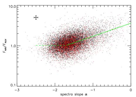
Figure 1: Correlation between $F_{\rm MIR}/F_{\rm NUV}$ and spectra slope $\alpha$. The black dots represent the 12483 objects in our primary sample and red dots represent the 3792 objects with only upper limits of W3 or/and W4 magnitudes. The green line displays the tendency predicted by SMC-like extinction, only for those $\alpha>-1.7$. The green dash line denotes the mean value of $F_{\rm MIR}/F_{\rm NUV}$ for quasars with $\alpha<-1.7$.

This correlation can be naturally interpreted as wavelength-dependent dust extinction. For example, Richards et al. (2001) showed that SDSS colors of quasars can be well represented by power laws of spectral indexes $\alpha=-1.5\pm 0.65$ with a red tail possibly due to dust extinctions. Because extinction is larger at shorter wavelengths, it makes the observed optical-UV spectrum flatter (redder), and simultaneously raises observed $F_{\rm MIR}/F_{\rm NUV}$. The large intrinsic scatters of $\alpha$ and $F_{\rm MIR}/F_{\rm NUV}$ dominate the variations at small $\alpha$ and small $F_{\rm MIR}/F_{\rm NUV}$, thus make the correlation weaker for blue sources as seen in Figure 1. Given that most blue quasars are likely not dust reddened, we check how the parameter $k$ changes with different $\alpha$ ranges. For the 7700 sources with $\alpha>-1.7$, we obtain $k_{1.7}=0.29\pm 0.02$, and for the 4505 sources with $\alpha>-1.5$, the result is $k_{1.5}=0.33\pm 0.02$.

By comparing the behaviours of radio-loud and radio-quiet quasars in our sample, we find that this $F_{\rm MIR}/F_{\rm NUV}$–$\alpha$ relation is independent of radio activities. Also, for the 3792 sources that are removed from our primary sample, we calculate their $F_{\rm MIR}$ using the same approach described in § 2.2 with the upper limits of W3 & W4 magnitudes provided in the WISE catalog, and find that they share the same behaviour as for the primary sample (the red dots in Fig. 1). Therefore, we will not distinguish these different categories of quasars when analyzing extinction effect below.

Previous studies suggested that dust extinction to quasars can be characterized by an SMC-like extinction curve (e.g. Richards et al., 2003; Hopkins et al., 2004; Gaskell et al., 2004). To illustrate the extinction effect on $F_{\rm MIR}/F_{\rm NUV}$–$\alpha$ relation quantitatively, we apply SMC-like extinction (Pei, 1992) of different values of $E(B-V)$ to an intrinsic blue QSO continuum, which is described by an intrinsic spectral slope $\beta$ ($F_{\lambda}\propto\lambda^{\beta}$) in the NUV range and a certain fraction of reprocessed infrared emission, to get a set of faked quasar continuua. We measure the NUV spectral slope ($\alpha$) and $F_{\rm NUV}$ for each faked continuum in exact the same way as that described above for real QSOs. It turns out that the relationship between $\alpha$ and $E(B-V)$ can be well described by a linear function,

$$E(B-V)=c\,(\alpha-\beta),$$ (3)

for $E(B-V)<0.3$. Particularly, for $\beta=-2.0$, we have $c=0.127$. For such a $E(B-V)$ range, the dust extinction has little effect on the $F_{\rm MIR}$, which can thus be considered as a constant. The relation between $\log(F_{\rm MIR}/F_{\rm NUV})$ and $\alpha$ for the mock quasars can be well described by a linear function with a slope of 0.322, independent of the value of $\beta$ for a wide range of $-2.2<\beta<-1.8$. This slope is also very close to the observed one $k_{1.7}=0.29$ or $k_{1.5}=0.33$. Therefore, our analysis supports that the observed $F_{\rm MIR}/F_{\rm NUV}$–$\alpha$ relation is statistically attributed to the dust extinction. And the scattering of this correlation is dominated by intrinsic dispersions of the continuum slope and $F_{\rm MIR}/F_{\rm NUV}$ (green lines in Fig. 1).

3.2 Extinction Correction for $F_{\rm NUV}$

In this subsection, we will correct $F_{\rm NUV}$ for dust extinction in a statistical way using the relation derived in the last section. First, we estimate the intrinsic distribution of $\log(F_{\rm MIR}/F_{\rm NUV})$ using blue quasars with $\alpha<-1.7$. As mentioned above, in this regime, extinction is small, and variations of $\log(F_{\rm MIR}/F_{\rm NUV})$ and $\alpha$ are dominated by intrinsic scatters, rather than reddening effect, albeit the latter must be present. The distribution of $\log(F_{\rm MIR}/F_{\rm NUV})$ for blue quasars can be well described by a Gaussian function with a mean value of 0.010 ($F_{\rm MIR}/F_{\rm NUV}=1.02$), and a dispersion of $\sigma=0.144$.

As we have shown in the last subsection, the dependence of $F_{\rm MIR}/F_{\rm NUV}$ on observed spectral slope $\alpha$ can be explained by dust extinction. Therefore, it is possible to correct $F_{\rm NUV}$ in a statistical way for the extinction using the derived $F_{\rm MIR}/F_{\rm NUV}$–$\alpha$ relation, with fitted spectral slope $\alpha$ as an extinction indicator. Assuming the mean $F_{\rm MIR}/F_{\rm NUV}$ at different $\alpha$ is the same (1.02) as that for blue quasars, and following the $F_{\rm MIR}/F_{\rm NUV}$–$\alpha$ relation derived in the last subsection, we calculate the correction factor for $F_{\rm NUV}$:

$$C=\left\{\begin{array}[]{ll}3.5\times 10^{0.322\times\alpha}&\mbox{if $\alpha>-1.7$}\\ 1&\mbox{if $\alpha<-1.7$}.\end{array}\right.$$ (4)

In the following analysis, we still use the notation $F_{\rm NUV}$ to denote the NUV flux, while it has already been corrected for extinction effect. It should be pointed out that this correction is only in statistical sense for the entire sample rather than for individual object since the intrinsic UV continuum slope $\beta$ and $F_{\rm MIR}/F_{\rm NUV}$ have fairly broad distributions. Nevertheless, by applying different cut on $\alpha$ as the standard for blue quasars, we estimate the uncertainty of this correction for individual object is less than 10%.

4 Warm Dust Covering Factor and its Relation with AGN Properties

4.1 Covering Factor of Warm Dust

The observed MIR flux $F_{\rm MIR}$ comes from three components: emission of the warm and hot dust heated by AGN, young-star emission at MIR band, and the emission of the accretion disc extending to MIR bands. Star-formation galaxies are characterized by strong PAH emission in MIR. Previous infrared spectroscopic studies suggest that PAH features are very weak in quasar spectra. Therefore, this component is not statistically important in our MIR range of rest-frame 3–10 $\mu$m. We will neglect it in the analysis hereafter. We estimate the accretion disc component by extrapolation of the optical/UV power-law corrected for reddening effect. This could be considered as an upper limit considering spectral flattening in the near-infrared due to starlight contribution in the SDSS spectrum. Numerically, the disc contribution to $F_{\rm MIR}$ is 5.2% of $F_{\rm NUV}$ for $\beta=-2.2$, 9.3% of $F_{\rm NUV}$ for $\beta=-2.0$ and 16.6% of $F_{\rm NUV}$ for $\beta=-1.8$. Since we focus on the MIR emission of the dust tori, we will subtract 0.093$F_{\rm NUV}$ from $F_{\rm MIR}$ to remove the contribution of the accretion disc and the slight starlight. The remained value, also denoting by $F_{\rm MIR}$, should be considered as the MIR emission of the warm dust.

Assuming that the NUV and MIR are isotropic, we can calculate the NUV luminosity $L_{\rm NUV}$ and MIR luminosity $L_{\rm MIR}$ from $F_{\rm NUV}$ and $F_{\rm MIR}$, respectively. Next, we consider the bolometric correction ($BC$) for the total luminosity from optical to X-ray. Since we have already corrected for extinction effect, we will use the mean SED of optically blue quasars in Richards et al. (2006) to calculate this correction. We calculate the $L_{\rm NUV}$ using the same method described in § 2.2, and integrate $\log(\nu f_{\nu})$ over $\log\nu$ from 1 $\mu$m to 10 keV to obtain the total luminosity in this range. This yields $BC=4.34$. Thus bolometric luminosities can be calculated by $L_{\rm bol}=BC\times L_{\rm NUV}$. Finally, we define the covering factor of warm dust as $\rm CF_{WD}=L_{\rm MIR}/L_{\rm bol}$. Our definition of covering factor is similar to that of Calderone et al. (2012), but different from theirs in the sense that we consider the IR flux in a fixed MIR range dominated by warm dust rather than the whole IR bands covered by WISE. Besides, we do not take into account anisotropic emission intentionally by this stage, while we will examine orientation effect in the last section.

4.2 Dependence of $\rm CF_{WD}$ on AGN Properties

In this subsection, we consider the relations between $\rm CF_{WD}$ and AGN properties: bolometric luminosity $L_{\rm bol}$, black hole mass $M_{\rm BH}$, and Eddington ratio $L/L_{\rm Edd}$. We present these relations for our sample in Fig. 2. We adopt the virial black hole masses in the catalog of Shen et al. (2011) with an additional extinction correction. These masses are estimated using the width of MgII $\lambda 2798$ and UV continuum luminosity at 2800 Å  (Eqn. (2) in Shen et al., 2011).

$$\log(\frac{M_{\rm BH,vir}}{M_{\odot}}) = a+b\,\log\,(\frac{\lambda L_{\lambda}}{10^{44}\,\rm erg\,s^{-1}})$$ (5)

$$+2\,\log(\frac{\rm FWHM}{\rm km\,s^{-1}}),$$

with $a=0.740$ and $b=0.62$. Shen et al. (2011) did not consider intrinsic extinction on the UV luminosity. In the following analysis, we will apply a correction by adding

$$\Delta=1.588*E(B-V)$$ (6)

to the value provided by Shen et al. (2011). This correction is calculated according to SMC reddening curve at 2800 Å. And $E(B-V)$ can be calculated from spectra slope ($\alpha$) using Eqn. (3) in § 3.1. Bolometric luminosities and black hole masses for the entire sample are also provided in the online table.

First, $\rm CF_{WD}$ is anti-correlated with $L_{\rm bol}$. The Spearman rank correlation coefficient ($R_{s}$) of this correlation is $-0.36$, indicating the anti-correlation is very significant ($P_{r}<10^{-6}$). A linear fit yields

$$\log\rm CF_{WD} = (-0.23\pm 0.02)\log L_{\rm bol}/(\rm erg\cdot s^{-1})$$ (7)

$$+(9.79\pm 0.04).$$

There is a significant anti-correlation between $\rm CF_{WD}$ and black hole mass $M_{\rm BH}$ with a Spearman rank correlation coefficient ($R_{s}=-0.27$, $P_{r}<10^{-6}$). A linear fit yields

$$\log\rm CF_{WD} = (-0.13\pm 0.02)\log(M_{\rm BH}/M_{\odot})$$ (8)

$$+(0.50\pm 0.02).$$

Finally, no apparent correlation is found between $\rm CF_{WD}$ and Eddington ratio,

$$\frac{L}{L_{\rm Edd}}=\frac{L_{\rm bol}}{1.5\times 10^{38}M_{\rm BH}}$$ (9)

($\rho=-0.008$ and $P_{r}=0.34$).

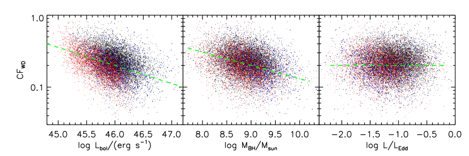
Figure 2: Relations between warm dust covering factor $\rm CF_{WD}$ and AGN properties: bolometric luminosity $L_{\rm bol}$ (left panel), black hole mass $M_{\rm BH}$ (middle panel), and accretion rate $L_{\rm bol}/L_{\rm Edd}$ (right panel). The meanings of black and red dots are exactly the same as in figure 1. The blue dots represent radio-loud quasars in the primary sample. The green dash lines represent the linear fit for these relations.

We compare radio-quiet and radio-loud quasars on these three diagrams, and find that they are indistinguishable. Particularly, we have fitted related parametres separately for the radio-loud subsample. First, the median value of $\rm CF_{WD}$ is consistent with that of the radio-quiet subsample within 10%. Second, the slopes of $\rm CF_{WD}$–$L_{\rm bol}$ and $\rm CF_{WD}$–$M_{\rm BH}$ relations are $-0.21\pm 0.02$ and $-0.15\pm 0.02$, respectively. The distribution of $\rm CF_{WD}$, and these fitting slopes are consistent with their 1 $\sigma$ uncertainties. Therefore, we conclude that none of these three relations are affected by radio activities.

Next, we consider the 3792 sources that only have upper limits of W3 and/or W4 magnitudes. From the left panel of Fig 2, it is obvious that these objects have systematically lower $L_{\rm bol}$, while at the same time their $\rm CF_{WD}$ (upper limits) are similar to those of quasars in our primary sample, so they shift to the left on the $\rm CF_{WD}$–$L_{\rm bol}$ diagram. In other words, they show systematically lower $\rm CF_{WD}$, comparing to the quasars of similar luminosities in the primary sample. Because the fraction of these sources is small, we get almost an identical slope for $\rm CF_{WD}$–$L_{\rm bol}$ relation for the entire sample. From the middle and right panels of Fig. 2, these quasars have similar distribution of black hole masses, but systematically lower $L/L_{\rm Edd}$ than the primary sample. However, they follow the same $\rm CF_{WD}$–$M_{\rm BH}$ and $\rm CF_{WD}$–$L/L_{\rm Edd}$ relations as the primary sample.

5 Discussion and Conclusion

5.1 On Radio-loud Quasars

Approximately 10% objects in our sample are radio-loud quasars. As we have discussed earlier, they exhibit the same correlations as radio-quiet quasars. Therefore, the majority of the radio-loud quasars have the very similar structure of accretion disc and dusty torus. This is consistent with Richards et al. (2006) and Shang et al. (2011) that mean SEDs of radio-quiet and radio-loud quasars in NUV and MIR are quite similar. However, it is of necessity to point out that a small fraction of the radio-loud quasars within our sample are blazars, in which the relativistic jets are beamed toward us. In this case, the relativistic jets would contribute significantly or even dominate the observed flux at near-ultraviolet and mid-infrared bands. Therefore, NUV and MIR emission in these objects will no longer represent the primary emission of the accretion discs and re-emission of the dusty tori. Thus our definition of warm dust covering factor is no long appropriate for these blazars. Nevertheless, the fraction of blazars in our whole sample is quite small ($\sim 1\%$ of type 1 quasars according to the argument of Padovani 2007), they will definitely not affect our conclusion.

5.2 Comparison with Previous Studies

In this work, we use the mid-infrared to near-UV luminosity ratio to estimate the covering factor of warm dust, and find a decrease of $\rm CF_{WD}$ with increasing $L_{\rm bol}$. Our results are in qualitative consistency with previous works.

Maiolino et al. (2007) estimated the dust covering factor for a few tens of QSOs using monochromatic flux ratio of 6.7$\mu$m to 5100Å, which is similar to our method in the spirit. However, their sample was constructed by merging two groups of QSOs from totally separate redshift ranges. Moreover, their analogous CF–$L_{\rm bol}$ correlation is far less significant when only considering either one group of objects with close redshifts. Therefore, their result might be hampered by possible evolution effect. A similar trend was obtained by Treister et al. (2008), who made use of nearly one hundred objects constructed from different surveys. In comparison with these works, our sample is much larger, and is uniformly selected in a relatively small redshift range.

More recently, Mor & Trakhtenbrot (2011) used the preliminary data release of WISE to study the hot dust component for a large and uniformly selected sample. Their definition of hot dust covering factor is quite similar to ours, and their results also revealed a dependence of hot dust CF on bolometric luminosity. Their sample covers a very wide redshift range and their hot dust luminosities were estimated using a certain dust model. Instead, we take a model-independent approach in our work. Similarly, Calderone et al. (2012) studied the dust covering factor for all radio-quiet AGNs constructed from WISE and SDSS within a small redshift range. These authors reported a similar trend of CF–$L_{\rm bol}$ relation by dividing the whole sample into three bins. Comparing with these studies, our work has taken the extinction effect into account. Also, we used the extinction-corrected broad band NUV luminosity, which is a better estimation of bolometric luminosity. Furthermore, we find that CF is significantly correlated with black hole mass, but is independent of Eddington ratio. The latter results are consistent with those reached by Cao (2005) for PG quasars.

In the literature, many authors used the fraction of type 2 objects as an indicator of total dust covering factor and reached a similar conclusion. For instance, Simpson (2005) and Hao & Strauss (2004) found a similar dependence of type 2 fraction on the [O III] luminosity using a magnitude-limited sample from the SDSS spectroscopic survey. Similar results were reported by other authors using sample constructed from flux-limited X-ray survey (e.g. Hasinger, 2008) or a combination of multi-band survey (Hatziminaoglou et al., 2009). However, some other authors have reported the opposite results. Lawrence & Elvis (2010) suggested that there is no correlation between type 2 fraction and [O III] luminosity after removing LINERs from the definition of type 2 objects, and so did Lu et al. (2010) by taking into account of various selection effects. A caution should be taken when comparing our results with those derived from the fraction of type 2 AGNs. We only consider the covering factor of warm dust, which is merely a portion of the obscuring material. Furthermore, a fraction of the type 2 objects are obscured by dust in their host galaxies rather than dust tori themselves (Goulding & Alexander, 2009).

5.3 Effects of Anisotropic Continuum

It should be emphasized that up to now, our whole analysis is based on the assumption that the NUV and MIR emission of quasars are isotropic. However, the NUV emission from a geometrically thin but optically thick accretion disc is predicted to be stronger at polar directions than at equatorial directions (e.g. Shakura & Sunyaev, 1973; Laor & Netzer, 1989; Fukue & Akizuki, 2006). If this is the case, our estimation of bolometric luminosity would be biased depending on the viewing angle (cf. Nemmen & Brotherton, 2010; Runnoe et al., 2012) and our definition of covering factor would certainly be inaccurate. For example, if an object is viewing relatively edge-on, we will underestimate its bolometric luminosity $L_{\rm bol}$ while overestimate its covering factor $\rm CF_{WD}$. In a statistical view, this can result in an anti-correlation between $\rm CF_{WD}$ and $L_{\rm bol}$, the same tendency as we have discovered from our sample.

To illustrate this more clearly, we construct a simple model to simulate the effect of different viewing angles. The simulation involves the same number of faked quasars as for our sample. We adopt three assumptions: (1) The intrinsic $\rm CF_{WD}$ and $L_{\rm bol}$ are independent, and obey log-normal distributions respectively. (2) The inclinations are random in a range of $1/2<\mu<1$, where $\mu=\cos\theta$ (the viewing angle). A lower limit on $\mu$ is set, since we require the line-of-sight must lie in the open angle of the torus, otherwise the NUV emission would be totally absorbed. The value 1/2 is corresponding to a type 2 to type 1 ratio of 1:1 (Lawrence & Elvis, 2010; Reyes et al., 2008). (3) The observed $L_{\rm bol}$ and $\rm CF_{WD}$ for each object are calculated from observed NUV flux and NIR/NUV flux ratio viewing from a certain direction. The dependence of NUV flux on viewing angle used in our model is

$$f(\mu)=f_{0}\times\mu\,(\mu+\frac{2}{3}),$$ (10)

following the results of Fukue & Akizuki (2006) who have taken into account limb darkening effect. Moreover, we require that the observed $L_{\rm bol}$ and $\rm CF_{WD}$ have exactly the same distribution as for our sample.

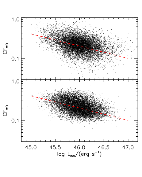
Figure 3: Above: the $\rm CF_{WD}$–$L_{\rm bol}$ relation for the primary sample. Bottom: the same relation for the simulated sample.

We plot our simulated $\rm CF_{WD}$–$L_{\rm bol}$ relation in Fig. 3, in comparison with the same relation of the sample. It turns out that our simulation obtains a similar but more compact relation. This seems to indicate that the observed $\rm CF_{WD}$–$L_{\rm bol}$ may result from anisotropic NUV continuum.

However, we stress that our simulation is initial and needs to be refined in several aspects. First, the assumption that the viewing angles are uniformly distributed is not satisfied by a flux-limited sample, such as the SDSS quasar sample used here. For example, a quasar close to the flux limit may move out of this limit if it is observed at a higher inclination. Thus it will be missed in the sample. In other words, the sample is biased against least luminous quasars at large inclinations. We note that the continuum flux decreases by a factor of 2.9 from $\mu=1$ to $\mu=1/2$, so this selection effect will significantly affect the inclination distribution of quasars with luminosities of a factor of 2.9 above the minimum value. The net effect will weaken the $\rm CF_{WD}$–$L_{\rm bol}$ correlation. In principal, we can incorporate this selection effect into the simulation by using the quasar luminosity function. However, we should understand that dust extinction is also coupled with the selection effect in the real case. Furthermore, dust extinction may or may not correlate with the inclination. If the absorber is the continuous extension of the dusty torus, there will certainly be a correlation; while on the other hand, if the absorption is due to the interstellar medium of the host galaxy, there may be no correlation. Because of lack of such detailed knowledge, we did not carry more complicated simulations.

Second, IR emission is also likely to be anisotropic due to the radiation transfer effect. According to the calculations of Nenkova et al. (2008a, b), for a typical clumpy dusty torus model, the MIR flux is $\sim 50\%$ weaker viewing from a 45 degree inclination than viewing from face-on direction. This factor is very similar to the anisotropy of NUV flux. In that case, the $\rm CF_{WD}$–$L_{\rm bol}$ relation will be much shallower due to the decrease of infrared flux viewing from higher inclinations. Hence the correlation will be weakened.

Therefore, although our simulation suggests that the observed $\rm CF_{WD}$–$L_{\rm bol}$ relation may be attributed to the inclination effect, there is fairly possible that the relation is intrinsic. A detailed study combining anisotropic radiation from both the discs and dust tori is very favourable in the future. Also, continuum variation on time scales of years will cause similar trend due to a delayed response of dust emission. The fact that CF is correlated with black hole mass but not correlated with Eddington ratio further indicates that luminosity dependence of CF is not solely due to the anisotropic emission alone.

To summarize, we use a complete sample in a narrow redshift range to study the warm dust emission of $\sim 16,000$ quasars. We correct for the dust extinction effect in a statistical way for the first time in this kind of study. We find that $\rm CF_{WD}$ is correlated with $L_{\rm bol}$ and $M_{BH}$, while not with Eddington ratio. Monte Carlo simulation suggests that $\rm CF_{WD}$–$L_{\rm bol}$ relation may be significantly affected by anisotropic disc emission. But it may not be the dominant factor for this relation.

Appendix

We present the primary data of all 16275 sources in our sample with an ASCII table as the supplementary material of this paper. The entire table is available online. Here we offer a small portion of the table for a guidance (Table 1).

Table 1: Primary data of our sample.

Name	Redshift	Spectra slope	NUV flux	MIR flux	$\rm CF_{WD}$	Bolometric luminosity	Black hole mass	Flagb	FIRST
(SDSS J)	($z$)	($-\alpha$)	($F_{\rm NUV}$a)	($F_{\rm MIR}$a)		$\log(L_{\rm bol}/(\rm erg\,s^{-1}))$	$\log(M_{\rm BH}/M_{\odot})$		flagc
000013.14+141034.6	0.958	1.657	2.773e-13	2.617e-13	0.217	45.757	8.800	0	-1
000024.02+152005.4	0.989	1.744	2.820e-13	2.044e-13	0.167	45.798	9.181	1	-1
000025.21+291609.2	0.924	1.718	8.433e-14	9.096e-14	0.249	45.201	8.216	0	-1
000025.93+242417.5	1.156	1.296	1.487e-13	2.077e-13	0.322	45.688	9.310	1	-1
000026.29+134604.6	0.768	1.691	3.206e-13	1.291e-13	0.093	45.582	8.670	1	-1
000028.82-102755.7	1.152	1.277	4.372e-13	2.150e-13	0.113	46.152	9.449	0	1
000031.86+010305.2	1.093	1.086	2.274e-13	3.818e-13	0.387	45.812	8.552	0	0
000042.89+005539.5	0.951	1.805	9.408e-13	1.033e-12	0.253	46.279	8.844	0	0
000057.67-085617.0	1.095	1.460	8.727e-13	8.643e-13	0.228	46.397	8.778	0	0
000123.96-102458.1	1.058	1.616	6.734e-13	6.254e-13	0.214	46.248	9.338	0	0
000123.98+284249.4	0.936	0.269	2.419e-13	2.935e-13	0.280	45.672	9.255	0	-1
000140.70+260425.5	0.765	1.385	3.656e-13	3.700e-13	0.233	45.636	8.670	0	-1
The full table including all 16275 sources is available online as supplementary material. A portion is shown here for guidance of its content.
a The flux is in unit of $\rm erg\,s^{-1}\,cm^{-2}\,\AA^{-1}$.
Here $F_{\rm NUV}$ refers to the value after extinction correction (see § 3) and $F_{\rm MIR}$ refers to the value after discounting the disc contribution (see § 4.1).
b Flag: 0=12483 source in our primary sample; 1=the rest 3792 sources which only have upper limits for W3 or W4 magnitudes.
c First flag: the same as column 15 in the catalog of Shen et al. (2011). -1=not in FIRST print; 0=FIRST undetected; 1=core dominant; 2=lobe dominant.

References

- Abazajian et al. (2009) Abazajian K. N., Adelman-McCarthy J. K., Agüeros M. A., et al., 2009, ApJS, 182, 543
- Antonucci (1993) Antonucci R., 1993, ARA&A, 31, 473
- Barthel (1989) Barthel, P. D. 1989, ApJ, 336, 606
- Becker et al. (1995) Becker R. H., White R. L., & Helfand D. J., 1995, ApJ, 450, 559
- Calderone et al. (2012) Calderone, G., Sbarrato, T., & Ghisellini, G., 2012, MNRAS, 425, L41
- Cao (2005) Cao X., 2005, ApJ, 619, 86
- Di Matteo et al. (2005) Di Matteo T., Springel V., & Hernquist L., 2005, Nat, 433, 604
- Elitzur (2008) Elitzur M., 2008, Mem. Soc. Astron. Italiana, 79, 1124
- Fitzpatrick (1999) Fitzpatrick E. L., 1999, PASP, 111, 63
- Fukue & Akizuki (2006) Fukue J., & Akizuki C., 2006, PASJ, 58, 1039
- Gaskell et al. (2004) Gaskell C. M., Goosmann R. W., Antonucci R. R. J., & Whysong D. H., 2004, ApJ, 616, 147
- Goulding & Alexander (2009) Goulding A. D., & Alexander D. M., 2009, MNRAS, 398, 1165
- Hao & Strauss (2004) Hao L., & Strauss M., 2004, AGN Physics with the Sloan Digital Sky Survey, 311, 445
- Hasinger et al. (2005) Hasinger G., Miyaji T., & Schmidt M., 2005, A&A, 441, 417
- Hasinger (2008) Hasinger G., 2008, A&A, 490, 905
- Hatziminaoglou et al. (2009) Hatziminaoglou E., Fritz J., & Jarrett T. H., 2009, MNRAS, 399, 1206
- Hopkins et al. (2004) Hopkins P. F., Strauss M. A., Hall P. B., et al., 2004, AJ, 128, 1112
- Hopkins et al. (2005) Hopkins P. F., Hernquist L., Cox T. J., et al., 2005, ApJ, 630, 705
- Krolik & Begelman (1986) Krolik J. H., Begelman M. C., 1986, ApJ, 308, L55
- Laor & Netzer (1989) Laor, A., & Netzer, H. 1989, MNRAS, 238, 897
- Lawrence (1991) Lawrence A., 1991, MNRAS, 252, 586
- Lawrence & Elvis (2010) Lawrence A., & Elvis M., 2010, ApJ, 714, 561
- Lu et al. (2010) Lu Y., Wang T.-G., Dong X.-B., & Zhou H.-Y., 2010, MNRAS, 404, 1761
- Maiolino et al. (2007) Maiolino R., Shemmer O., Imanishi M., et al., 2007, A&A, 468, 979
- Mor & Trakhtenbrot (2011) Mor R., & Trakhtenbrot B., 2011, ApJ, 737, L36
- Nemmen & Brotherton (2010) Nemmen, R. S., & Brotherton, M. S. 2010, MNRAS, 408, 1598
- Nenkova et al. (2008a) Nenkova M., Sirocky M. M., Ivezić Ž., & Elitzur M., 2008, ApJ, 685, 147
- Nenkova et al. (2008b) Nenkova M., Sirocky M. M., Nikutta R., Ivezić Ž., & Elitzur M., 2008, ApJ, 685, 160
- Netzer & Laor (1993) Netzer H., & Laor A., 1993, ApJ, 404, L51
- Padovani (2007) Padovani, P. 2007, The First GLAST Symposium, 921, 19
- Pei (1992) Pei Y. C., 1992, ApJ, 395, 130
- Pogge (1988) Pogge R. W., 1988, ApJ, 328, 519
- Reyes et al. (2008) Reyes, R., Zakamska, N. L., Strauss, M. A., et al., 2008, AJ, 136, 2373
- Richards et al. (2001) Richards, G. T., Fan, X., Schneider, D. P., et al., 2001, AJ, 121, 2308
- Richards et al. (2003) Richards G. T., Hall P. B., Vanden Berk D. E., et al., 2003, AJ, 126, 1131
- Richards et al. (2006) Richards G. T., Lacy M., Storrie-Lombardi L. J., et al., 2006, ApJS, 166, 470
- Runnoe et al. (2012) Runnoe, J. C., Brotherton, M. S., & Shang, Z. 2012, MNRAS, 422, 478
- Sako et al. (2000) Sako M., Kahn S. M., Paerels F., & Liedahl D. A., 2000, ApJ, 543, L115
- Schlegel et al. (1998) Schlegel D. J., Finkbeiner D. P., & Davis M., 1998, ApJ, 500, 525
- Schneider et al. (2010) Schneider D. P., Richards G. T., Hall P. B., et al., 2010, AJ, 139, 2360
- Simpson (2005) Simpson C., 2005, MNRAS, 360, 565
- Shakura & Sunyaev (1973) Shakura N. I., & Sunyaev R. A., 1973, A&A, 24, 337
- Shang et al. (2011) Shang Z., Brotherton M. S., Wills B. J., et al., 2011, ApJS, 196, 2
- Shen et al. (2011) Shen Y., Richards G. T., Strauss M. A., et al., 2011, ApJS, 194, 45
- Stern & Laor (2012) Stern, J., & Laor, A. 2012, MNRAS, 423, 600
- Treister et al. (2008) Treister E., Krolik J. H., & Dullemond C., 2008, ApJ, 679, 140
- Vanden Berk et al. (2001) Vanden Berk D. E., Richards G. T., Bauer A., et al., 2001, AJ, 122, 549
- White et al. (1997) White, R. L., Becker, R. H., Helfand, D. J., & Gregg, M. D., 1997, ApJ, 475, 479
- Wilson & Ulvestad (1983) Wilson A. S., & Ulvestad J. S., 1983, ApJ, 275, 8
- Wright et al. (2010) Wright E. L., Eisenhardt P. R. M., Mainzer A. K., et al., 2010, AJ, 140, 1868
- Zheng et al. (1997) Zheng W., Kriss G. A., Telfer R. C., Grimes J. P., & Davidsen A. F., 1997, ApJ, 475, 469