Forecasting the underlying potential governing the time series of a dynamical system

Abstract

We introduce a technique of time series analysis, potential forecasting, which is based on dynamical propagation of the probability density of time series. We employ polynomial coefficients of the orthogonal approximation of the empirical probability distribution and extrapolate them in order to forecast the future probability distribution of data. The method is tested on artificial data, used for hindcasting observed climate data, and then applied to forecast Arctic sea-ice time series. The proposed methodology completes a framework for ‘potential analysis’ of tipping points which altogether serves anticipating, detecting and forecasting non-linear changes including bifurcations using several independent techniques of time series analysis. Although being applied to climatological series in the present paper, the method is very general and can be used to forecast dynamics in time series of any origin.

1 Introduction

Many dynamical systems in general, and geophysical subsystems in particular, lack analytical deterministic descriptions with fully developed physical models, being represented mainly by recorded time series. At the same time such systems may be of great public interest and societal impact, such as the current climate change with rising temperature records around the globe.

In these circumstances, powerful research tools may be provided by statistical time series analysis (Priestley, 1981; Tong, 1990; Box et al, 2008), which have found entry into the analysis of climate data from a general viewpoint (Mudelsee, 2010) and also from a nonlinear dynamical system viewpoint (Donner and Barbosa, 2008). In particular, system dynamics can be approximated by means of simple generalised stochastic models, where uncertain or unknown variables are represented by stochastic components (Hasselmann, 1976; Chan and Tong, 2001). Of specific regard to the present paper are time series analysis methods that deal with correlations and scaling of fluctuations (Peng et al, 1994; Podobnik and Stanley, 2008; Laloux et al, 1999; Plerou et al, 1999; Koscielny et al, 1996; Fraedrich and Blender, 2003).

In previous papers (Livina and Lenton, 2007; Livina et al., 2010, 2011), we have developed several time series techniques for anticipating and detecting ’tipping points’ in trajectories of dynamical systems, with applications in climatology. Modified ’degenerate fingerprinting’ (Livina and Lenton, 2007) was introduced for early warning of critical behaviour in time series to allow one to anticipate an upcoming bifurcation or transition (climate tipping points (Lenton et al., 2008)). This was based on ’degenerate fingerprinting’ (Held and Kleinen, 2004), where the decay rate in the series is monitored using lag-1 autocorrelation in an autoregressive model (AR1). Modified degenerate fingerprinting employs Detrended Fluctuation Analysis for the same purposes. For noisy time series, we developed the method of potential analysis (Livina et al., 2010, 2011), which derives the number of system states under the assumption of quasi-stationarity of a data subset. This can distinguish a transition, which may be a forced drifting of the record without structural changes in the fluctuations, from a bifurcation which happens when the underlying system potential (the system states that a climate variable may sample) changes in structure, e.g. instead of two potential wells one or three wells appear. A bifurcation is characterised by structural change in the dynamical system, whereas transitional series preserve the same structure of fluctuations.

If both techniques give indication of dynamical change, this denotes a genuine bifurcation. If modified degenerate fingerprinting indicates a change but potential analysis does not, this means a transition rather than a bifurcation, with no changes in the underlying system potential.

In this paper, we develop the methodology further, so that we become able to not only anticipate and detect, but also to forecast the time series dynamics. The skill of such a forecast will depend on several factors, in particular, whether the upcoming change will be gradual or abrupt, at what rate it will be happening and how the scaling properties of the stochastic component may change with time.

Here we outline the methodology, test it on artificial data, in several hindcast case studies, and provide a forecast of the dynamics of Arctic sea-ice extent in the nearest future.

2 Methodology

2.1 Potential analysis as the basis of the method

We consider a simple stochastic model with a polynomial potential $U$ as an approximation of the system dynamics,

$$\dot{x}(t)=-U^{\prime}(x)+\sigma\eta,$$ (1)

where $\dot{x}$ is the time derivative of the system variable $x(t)$ (time series of an observed variable), $\eta$ is Gaussian white noise of unit variance and $\sigma$ is the noise level. In the case of a double-well potential, it can be approximated by a polynomial of 4th order:

$$U(x)=a_{4}x^{4}+a_{3}x^{3}+a_{2}x^{2}+a_{1}x.$$

According to the Fokker-Planck equation for the dynamic evolution of the probability density function $p(x,t)$,

$$\partial_{t}p(x,t)=\partial_{x}[U^{\prime}(x)p(x,t)]+\frac{1}{2}\sigma^{2}\partial_{x}^{2}p(x,t)$$ (2)

its stationary solution is given by (Gardiner, 2004)

$$p(x)\sim\exp[-2U(x)/\sigma^{2}].$$ (3)

The potential can be reconstructed from time series data of the system as

$$U(x)=-\frac{\sigma^{2}}{2}\log p_{\rm d}(x),$$ (4)

which means that the empirical probability density $p_{\rm d}$ has the number of modes corresponding to the number of wells of the potential.

This simple approximative approach allowed us to reconstruct the system potential of various climatic records (see (Livina et al., 2011)). It works with remarkable accuracy for data subsets of length as short as 400 to 500 data points, demonstrating above 90% rate of accurate detection, as was shown in an experiment with artificial data. For data subsets of length above 1000 points it correctly detects the structure of the potential with a rate of 98% (Livina et al., 2011). Potential analysis was introduced in (Livina et al., 2010) which is an open-access paper published by Copernicus.org; this makes it easily accessible for the broad readership and more details on the methodology can be found there.

Here we develop the potential method beyond its detection capability, such that we are able to forecast the behaviour of a time series on the basis of its potential. To that effect, we introduce an extrapolation technique that would use the potential structure of the time series with linear extrapolation of the coefficients of the approximating polynomials. To reduce the biases introduced during various stages of the potential analysis (due to kernel distribution approximation, further logarithmic transformation, noise estimation, and finally polynomial fits), we use the empirical probability density rather than its logarithmic transformation, the potential (see Eq. 4). Moreover, unlike in previous work (Livina et al., 2011), we use not the $2N$ potential coefficients (where $N$ is the number of potential wells) but the coefficients of the approximation of the empirical probability density by a finite Chebyshev polynomial series (following the approach of (Neagoe, 1990)). Chebyshev approximation has an advantage of being near optimal, and already 10th-degree approximation in most cases of observed time series provides an accurate fit with low values of the error function.

2.2 Approximation of the probability density

To approximate the empirical probability density, we use the orthogonal (in the interval $[-1,1]$) Chebyshev polynomials of the first kind:

$$\begin{array}[]{l}T_{0}(x)=1,\\[10.0pt] T_{1}(x)=x,\\[10.0pt] \dots\\[10.0pt] T_{n+1}(x)=2xT_{n}(x)-T_{n-1}(x).\end{array}$$ (5)

The polynomial $T_{n}(x)$ has $n$ zeros in the interval $[-1,1]$ at points

$$x=\cos\left(\frac{\pi(k-1/2)}{n}\right),\quad k=1,2,\ \dots,\ n.$$

The approximation of a function $f(x)$ can be done by using a truncated (finite $N$) sum of the following form

$$f(x)\cong\left(\sum\limits_{k=0}^{N-1}c_{k}T_{k}(x)\right)-\frac{1}{2}c_{0},$$ (6)

where $c_{k}$ are the coefficients obtained by discrete cosine transform of the vector of nonuniformly spaced samples of the considered function over the sampling grid

$$x_{k}=\cos\left(\frac{\pi(k-1/2)}{n}\right),\quad k=1,2,\,\dots\,,n.$$

For an arbitrary interval $[a,b]$ it is necessary to transform variables as

$$y=\frac{x-0.5\cdot(b+a)}{0.5\cdot(b-a)}.$$

A good example of the above calculations is given in (Neagoe, 1990).

When decomposition (6) is obtained according to the particular time series problem to be analysed, the resulting polynomial is expanded, thus producing the final coefficients

$$f(x)\cong\left(\sum\limits_{k=0}^{N-1}\tilde{C}_{k}x^{k}\right).$$ (7)

2.3 Linear extrapolation of the coefficients and forecast time series

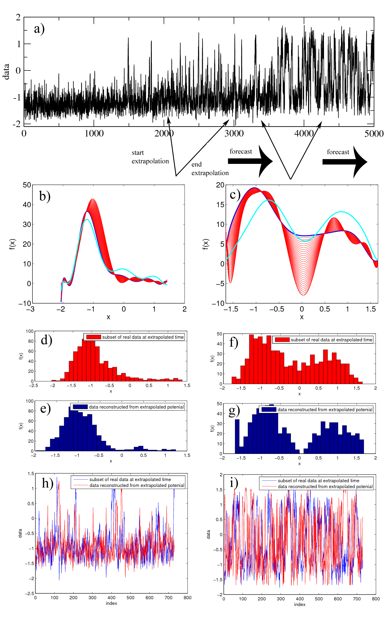
We consider the approximation of the empirical probability density using Chebyshev polynomials $T_{0},\,\dots\,,T_{10}$. When the approximating polynomial is derived, the decomposition coefficients $\tilde{C}_{k}$ (Eq. 7) are linearly extrapolated using a set of preceding values. The interval of these, as well as the extension of the extrapolated interval can be chosen according to the particular time series to be analysed. If the series dynamics is homogeneous and steady, the horizon of the forecast may be as far as several decades of daily data (i.e., thousands of points). If the dynamics is highly nonlinear and abrupt, the horizon of the forecast may be very short, and the forecast probability density function may differ significantly from the observed one at the end of the forecast interval. However, even in this case, although the pdfs may differ, the simulated time series — due to the sampling in the close domain and sorting according to the observed data — is realistically similar to the hindcast data (see the example of artificial data in Fig. 3). As a rule of thumb, the horizon of forecast may be chosen at the scale of several hundreds up to several thousand points, which in case of daily data means up to 10 years of forecast horizon.

The initial pdfs (those providing sequences of potential coefficients to be extrapolated) are estimated for fixed time interval, in a sequence of subsets prior to the forecast starting point (in sliding windows). The extrapolation of parameters provides adequate scaling of the pdf, and no further normalisation is necessary.

Once a new probability density is calculated, we generate a forecast time series using a rejection sampling algorithm (see, for instance, (Gilks and Wild, 1992)). This provides an artificial series with the prescribed distribution, but this may be not enough for obtaining a realistic forecast time series, because the ordering of the series (and hence scaling properties like long-term memory) should be reconstructed according to the initial data. For this purpose, we apply so-called ”sorting” of the time series, that means arranging its values in the same order as in the initial data (before the forecast started), thus reproducing realistic correlations (because their distributions are already very similar due to the extrapolation of probability density). Sorting is a simple numerical algorithm which uses ranking of the values of two series, initial subsample and forecast subsample. However, this should be done with care, especially in data with seasonality: if there is a seasonal trend, it is very important to sort the forecast series according to observed data at the same date of the year, so that further seasonal variability would be adequate. This is achieved by going back along the series with a step equal to the seasonality period (365 for daily data or 12 for monthly data). Since certain years may be anomalous in fluctuations (due to internal variability in the system), the initial data used for sorting may be an average over several years starting from the same date in a year (for instance, March 1st in several consecutive years). This average is then used to sort the forecast series starting on March 1st and projecting into the future.

2.4 Uncertainties and applicability; criteria of performance

It is necessary to note that minor uncertainties are introduced at various steps of the forecasting algorithm: first when the potential stochastic model is used as an approximation of dynamics, then when the empirical probability density is approximated by Chebyshev polynomials (minor outliers); furthermore, the polynomial coefficients are linearly extrapolated, which means that the actual dynamics is correctly forecast only in the case of linear evolution of such coefficients.

In many cases of abrupt highly nonlinear dynamics the linear extrapolation of the decomposition coefficients may produce an empirical distribution with large deviations, especially in case of non-stationarity of the data. We attempted bootstrapping of the decomposition of coefficients according to (Mudelsee, 2010). Based on bootstrapping techniques, it is possible to consider blocks of data in a chosen subset $x$ of size

$$L=NINT\left(W^{1/3}\frac{\sqrt{6}a_{1}(x-\bar{x})}{1-(a_{1}(x-\bar{x}))^{2}}\right),$$ (8)

where $NINT(\cdot)$ is the nearest integer function, $W$ is the window length, $a_{1}$ is the lag-1 autocorrelation, $\bar{x}$ is the mean value of the subset $x$. This block length selector was derived in (Mudelsee, 2010) from (Sherman et al, 1998), who adapted a formula from (Carlstein, 1986). For $a_{1}\to 0$, $L$ is chosen equal to 1; when the denominator of Eq. (8) tends to 0, $L$ is chosen equal to $N-1$.

In the case of nonstationary data, when the probability distribution varies within the data subset, bootstrapping provides estimates of the partial probability distributions, which may deviate from the average quite significantly. In practical terms, applying bootstrapping for estimation of the decomposition coefficients in non-stationary data provided worse results in the considered samples, with the forecast time series of poorer skill than the single-estimated probability density functions. A possible solution to this could be modification of the bootstraping algorithm, where instead of mean value removal a more sophisticated detrending is applied. We plan to adapt block bootstrap methods (Mudelsee, 2010) (Chapter 3 therein) for that means in a future study.

Furthermore, the important parameter that affects the skill of the forecast is the extrapolation period. The skill of the forecast drops with increase of its value.

Obviously, in the case of abrupt changes using linear extrapolation of coefficients may prove unsatisfactory, and our method in those cases may be not applicable. The best results are obtained when the data undergoes gradual dynamic change and the forecast horizon is within 100 time units (which means 3 months for daily data and up to 8 years for monthly data).

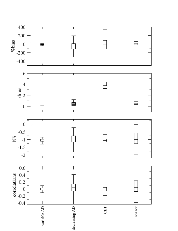
To assess the skill of the forecast, we used several techniques widely applied in modelling community for comparison of observed and modelled data, for instance, in hydrology (Nash and Sutcliffe, 1970; Livina et al., 2007):

$$\begin{array}[]{ll}\mbox{Daily Root Mean Square}&\sqrt{\frac{1}{n}\sum_{i=1}^{N}(x_{m}^{i}-x_{o}^{i})^{2}},\\[10.0pt] \mbox{Nash-Sutcliffe efficiency}&1-\left(\sum_{i=1}^{N}(x_{m}^{i}-x_{o}^{i})^{2}\left/\sum_{i=1}^{N}(x_{o}^{i}-\overline{x})^{2}\right.\right),\\[10.0pt] \mbox{Percent bias}&\left[\sum_{i=1}^{N}(x_{m}^{i}-x_{o}^{i})\left/\sum_{i=1}^{N}(x_{o}^{i})\right.\right]\times 100,\end{array}$$

where $x_{o}$ and $x_{m}$ are the observed and modelled series, respectively, $i=1,\,\dots,\,N$ is time index, $\overline{x}$ is the mean value of the series $x$. It is easy to see that for two identical time series DRMS=0, NS=1, and %bias=0, and any deviation from those values would indicate the difference between the modelled and observed time series pointwise.

However, it is necessary to mention that these skill estimators perform best when applied to data with normal distribution without outliers, which is not the case in most of our datasets; therefore, they may introduce additional biases in estimation of accuracy of arbitrary data; we apply them for general information only.

3 Tests of artificial and climate data

3.1 Artificial data

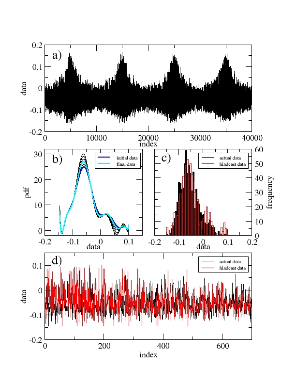
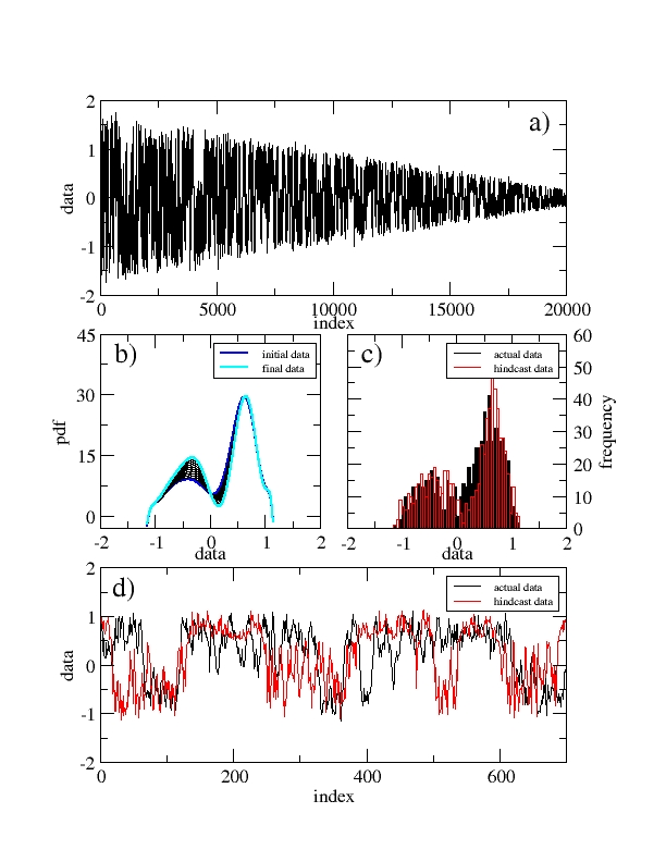
We considered several simulated time series: an artificial dataset where the potential is varying from single-well to double-well and back several times (Fig. 1), double-well-potential data with decreasing noise level (Fig. 2) and artificial data bifurcating from one-well- to double-well-potential (simulated tipping point, Fig. 3). Our aim is to test if the proposed methodology is capable to capture the modelled dynamics of the series and forecast the record adequately.

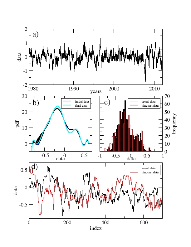
We perform hindcast of these series by choosing a certain point where we start extrapolation of the empirical probability density, then we compare the modelled series with actual data at the end of the forecast. Figures 1 and 2 show datasets in panels (a), the probability density functions and histograms of the data and hindcast in panels (b, c) of each plot, and the samples of modelled data in panels (d).

Figure 3 combines two hindcasts of the series bifurcating from one-well to double-well potential, in the intervals shown by arrows in the figure (probability density functions and histogram of observed and modelled data in panels (b, d, e, h) and (c, f, g, i)). The initial potential is $U(x)=x^{4}-2x^{2}$; then the term with 1st power of $x$ starts growing gradually from zero until the potential reaches form $U(x)=x^{4}-2x^{2}+8x$. In this experiment, the forecast is performed in total for 1530 “days” without any intermediate assimilation of modelled data, and for these conditions the modelled series is very close in statistical properties to the hindcast data (although the probability density is not entirely identical). The result demonstrates that for certain bifurcating systems with gradual dynamics the methodology may be very efficient as a forecast tool.

3.2 Climate data

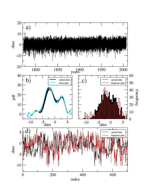
Similarly to artificial data in the previous section, we performed hindcast experiments with observed climate data, temperature and sea-ice extent. The results are shown in Figures 4,5.

The Central England Temperature (Manley, 1974; Parker et al, 1992), which is available as monthly series since 1659 and as daily since 1772, is considered here in daily format. It is first deseasonalised (subtracting the average annual cycle of daily data) and then the hindcast is performed as in the above artificial records.

Sea ice area data were obtained from ‘The Cryosphere Today’ project of the University of Illinois. This dataset uses SSM/I and SMMR series satellite products and spans 1979 to present at daily resolution. The fluctuations of the Arctic sea-ice area are not only deseasonalised, but also the quadratic trend is removed, as we pre-processed the sea-ice data in our recent paper (Livina and Lenton, 2013). This was done to study the properties of the fluctuations.

Altough the real data has much more complicated variability and dynamics, the method performs as well as in the cases of artificial data analysed above, with modelled series having the same statistical properties as the initial data.

3.3 Forecast skill

The skill of the forecast is calculated for multiple subsets along series using the hindcast approach as described above. We show the skill in Figure 6 as boxplots with whiskers (outliers are not shown) and conclude that in some cases the exact statistical properties and correlations are not reproduced well, with acceptable mean values over subsets but rather large standard deviations. This is because our stochastic approach is based on the probability density function, which means that the exact dynamics may vary for series with the same histograms, and skill estimators based on point-wise comparison of time series may deviate from ideal values. However, the patterns of the series are very close and suitable for long-term stochastic predictions, as we show below for the Arctic sea-ice.

The stochastic forecast is not expected to be precise at particular values. For example, even the sophisticated deterministic climate models still struggle to forecast actual weather at medium-term scale. Our forecast technique is much lighter computationally, being based on a simple stochastic model; yet it reproduces the pattern of the series and takes into account typical seasonal variability from the past, which produces realistic forecast series. There exist regional climate models that achieve good accuracy of forecast, but those usually implement assimilation of observational data, which cannot be done when attempting longer-timescale forecast.

4 Future Arctic sea-ice area dynamics

Arctic sea-ice dynamics have been a topic of recent scientific debate, and available estimates of when summer ice cover will disappear range from as early as 2016 to never; the early ice loss estimate comes from extrapolation of PIOMAS data (Zhang et al, 2010; Wang and Overland, 2009; Boe et al, 2009).

There is also an ongoing debate about whether tipping points could occur in the Arctic region (see (Serreze, 2011; Tietsche, 2011; Wassman and Lenton, 2012; Lenton, 2012) and references therein). Several studies argue that sea-ice loss is highly reversible and therefore not a tipping point (Tietsche, 2011). Others suggest that reversible tipping points can occur and summer sea-ice loss may be one candidate (Lenton et al., 2008). Here we restrict ourselves to the question of when summer ice cover is forecast to disappear in the Arctic.

Here we propose a stochastic forecast based on the above methodology, without taking into account complex feedbacks (that may reverse the declining dynamics as well as speed it up). Assuming that the present dynamics continues its gradual development, and taking into account what we already know about this time series, we forecast it using potential analysis.

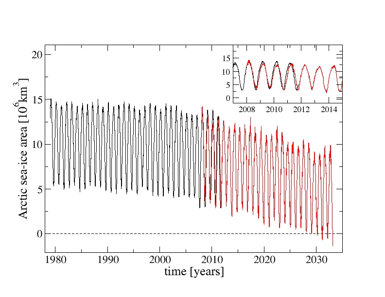
In Fig. 7, we show a long-term forecast of the Arctic sea-ice by combining our knowledge about seasonality and current trends in the data. From the point of forecast (which is chosen in 2008 rather than most recently in order to assess the accuracy of the forecast over the recently observed data), we combine the last 5-year seasonal average, extrapolated quadratic trend, and the forecast of the fluctuations as described above. In the inset we show that between 2008 and 2010 the forecast is surprisingly good and very close to the observed data; the later departure is mainly due to very anomalous summers in the recent few years.

The forecast indicates complete loss of Arctic summer sea-ice area by the 2030s. Obviously, the method provides an estimate of sea ice loss in the Arctic Ocean if the system will not experience new feedbacks which are not included in our approach. It is therefore a conservative estimate solely based on extrapolation of the current trends.

5 Discussion.

We have developed a forecasting technique based on potential analysis with dynamical propagation of the probability density. As the main idea, we employ approximations of the empirical probability distributions and extrapolate them to the future probability distribution of data. We conducted experiments with artificial, model and observed climatic data and showed the efficient forecast performance of the new methodology.

As one particular example, we applied the method to the expected sea ice trend in the Arctic Ocean. The dynamics of Arctic sea ice was forecast and shown to disappear in summer in the 2030s if the current trends remain the same. This can be compared to fully dynamical models.

As a logical next step, bootstrap resampling (Section 2.4) can help to construct prediction confidence intervals based on percentiles or standard errors (Mudelsee, 2010).

Acknowledgement. The idea of the paper was developed during VNL’s visit to Alfred Wegener Institute for Polar Research, Germany (February 2012). VNL and TML were supported by NERC through the project ”Detecting and classifying bifurcations in the climate system” (NE/F005474/1) and by AXA Research Fund through a postdoctoral fellowship. MM is supported by the European Commission as PI in the Marie Curie Initial Training Network LINC (project number 289447) under the Seventh Framework Programme. The Central England Temperature dataset was provided by the British Atmospheric Data Centre (BADC), which is part of the NERC National Centre for Atmospheric Science (NCAS). The research was carried out on the High Performance Computing Cluster supported by the Research Computing Service at the University of East Anglia.

Figure 1: Artificial data with oscillating potential, from one to two wells and back: a) time series; b) hindcast empirical probability density (Chebyshev-polynomial approximations, which may result in some negative pdf values), where blue curve is the initial statistics at the beginning of the hindcast, black curves are extrapolated densities up to 100 time units ahead, cyan curve is the real pdf at the end of the forecast, for comparison with extrapolation; c) histograms of the forecast and real data at the end of extrapolation; d) time series corresponding to histograms in the panel c).

Figure 2: As in Fig. 1, for artificial double-well-potential data with decreasing noise level.

Figure 3: Artificial data bifurcating from one-well to double-well dynamics — two hindcasts are demonstrated. The first hindcast, from point 2100, has initial potential ending at 2100 and the final potential (for the hindcast comparison) starting after 800 points of extrapolation, that is, at 2900. Start and end of the extrapolation are indicated by two thin arrows under the top panel. After this, the forecast is running for 730 days ending at 3630, which is indicated by the thick line underneath. Panels: a) time series – the dynamics is potentially extrapolated in two intervals: from 2100 to 2900 and from 3400 to 4200; b) emprical probability density (Chebyshev-polynomial approximations) for the interval from 2100 to 2900: blue curve is the initial probability density, cyan is the final curve; red curves are extrapolated at equal steps; c) the same as (b) for the interval from 3400 to 4200; (d) and (e) are histograms for extrapolation at point 2900: comparison of the actual histogram and the result of extrapolation; (f) and (g) are the same as (d) and (e) for the point 4200; h) comparison of the forecast and actual data in interval from 2900 to 3630: i) comparison of the forecast and actual data in interval from 4200 to 4930.

Figure 4: Central England Temperature deseasonalised fluctuations: a) time series; b) hindcast empirical probability density (Chebyshev-polynomial approximations), where blue curve is the initial statistics at the beginning of the hindcast, black curves are extrapolated densities up to 100 time units ahead, cyan curve is the real pdf at the end of the forecast, for comparison with extrapolation; c) histograms of 2-year-long hindcast: the forecast and real data at the end of extrapolation; d) time series corresponding to histograms in the panel (c).

Figure 5: As in Fig. 4, for Arctic sea-ice area fluctuations after deseasonalising and removal of quadratic decreasing trend.

Figure 6: The skill statistics of the forecasts of four datasets. Outliers are not shown. ’Variable AD’ is the dataset analysed in Fig. 1; ’Decreasing AD’ is the dataset analysed in Fig. 2; ’CET’ is the dataset analysed in Fig. 4; ’sea ice’ is the dataset analysed in Fig. 5.

Figure 7: Arctic sea-ice area forecast until 2035, which indicates zero level of summer sea ice in the 2030s. The inset plot shows magnification of the main plot for the period 2007-2015, where one can see how the forecast series (red) is started from 2008 and extends beyond the observed data (black).

References

- Priestley (1981) Priestley M.B. (1981), Spectral Analysis and Time Series. Academic Press, London. 890 pages.
- Tong (1990) Tong H. (1990), Non-linear Time Series. Clarendon Press, Oxford. 564 pages.
- Box et al (2008) Box E. P., G. M. Jenkins, and G. C. Reinsel (2008), Time Series Analysis: Forecasting and Control, Wiley, 4th edition.
- Mudelsee (2010) Mudelsee M. (2010), Climate Time Series Analysis: Classical Statistical and Bootstrap Methods, Springer, 474p.
- Donner and Barbosa (2008) Donner R.V., S.M. Barbosa (Eds.) (2008), Nonlinear Time Series Analysis in the Geosciences: Applications in Climatology, Geodynamics and Solar–Terrestrial Physics. Springer, Berlin. 390 pages.
- Hasselmann (1976) Hasselmann K., Stochastic climate models: Theory, Tellus XXVIII (6), 473–484.
- Chan and Tong (2001) Chan K,-S. and H. Tong (2001), Chaos: A Statistical Perspective. Springer, New York. 300 pages.
- Peng et al (1994) Peng C.- K., S. V. Buldyrev, S. Havlin, M. Simons, H. E. Stanley, and A. L. Goldberger (1994), Mosaic organization of DNA nucleotides, Phys. Rev. E 49, 1685–1689.
- Podobnik and Stanley (2008) Podobnik B. and H. E. Stanley (2008), Detrended Cross-Correlation Analysis: A new method for analyzing two non-stationary time series, Phys. Rev. Lett. 100, 084102.
- Laloux et al (1999) Laloux L., P. Cizeau P., J. P. Bouchaud, M. Potters (1999), Noise dressing of financial correlation matrices, Phys. Rev. Lett. 83, 1467;
- Plerou et al (1999) Plerou V., P. Gopikrishnan, B. Rosenow, L. A. N. Amaral, and H. E. Stanley, Universal and nonuniversal properties of cross correlations in financial time series, Phys. Rev. Lett. 83, 1471 (1999).
- Koscielny et al (1996) Koscielny-Bunde E., A.Bunde, S.Havlin, Y.Goldreich (1996), Analysis of daily temperature fluctuations, Physica A 231(4), 393-396.
- Fraedrich and Blender (2003) Fraedrich K. and R. Blender (2003), Scaling of atmosphere and ocean temperature correlations in observations and climate models, Phys. Rev. L. 90(10), 108501 (doi:10.1103/PhysRevLett.90.108501).
- Livina and Lenton (2007) Livina V. and T. Lenton (2007), A modified method for detecting incipient bifurcations in a dynamical system, Geophys. Res. Lett. 34 (3), L03712.
- Livina et al. (2010) Livina, V. N., F. Kwasniok, F., and T. M. Lenton (2010), Potential analysis reveals changing number of climate states during the last 60 kyr, Climate of the Past 6, 77-82.
- Livina et al. (2011) Livina V. N., F. Kwasniok, G. Lohmann, J. W. Kantelhardt, and T. M. Lenton (2011), Changing climate states and stability: from Pliocene to present, Climate Dynamics 37 (11-12), 2437-2453, DOI: 10.1007/s00382-010-0980-2.
- Lenton et al. (2008) Lenton, T. M. et al. (2008), Tipping elements in the Earth’s climate system, Proc. Nat. Acad. Sci USA 105 (6), 1786-1793, doi:10.1073/pnas.0705414105.
- Held and Kleinen (2004) Held H. and T. Kleinen (2004), Detection of climate system bifurcations by degenerate fingerprinting, Geophys. Rev. Lett. 31, L23207.
- Gardiner (2004) Gardiner C. W. (2004), Handbook of Stochastic Methods, 3rd ed., 415pp., Springer.
- Neagoe (1990) Neagoe V.-E. (1990), Chebyshev nonuniform sampling cascaded with the discrete cosine transform for optimum interpolation, IEEE Transactions on Acoustics, Speech and Signal Processing 38 (10), 1812–1815.
- Gilks and Wild (1992) Gilks W. and P. Wild (1992), Adaptive rejection sampling for Gibbs sampling, Applied Statistics - Journal of the Royal Statistical Society Series C 41 (2), 337–348.
- Sherman et al (1998) Sherman M., F. M. Speed Jr., F. M. Speed (1998), Analysis of tidal data via the blockwise bootstrap Journal of Applied Statistics 25(3), 333 340.
- Carlstein (1986) Carlstein E. (1986), The use of subseries values for estimating the variance of a general statistic from a stationary sequence, The Annals of Statistics 14(3), 1171–1179.
- Nash and Sutcliffe (1970) Nash J. E. and J. V. Sutcliffe (1970), River flow forecasting through conceptual models part I - A discussion of principles, Journal of Hydrology 10 (3), 282-290.
- Livina et al. (2007) Livina V., Z. Kizner, P. Braun, T. Molnar, A. Bunde, S. Havlin (2007), Temporal scaling comparison of real hydrological data and model runoff records, Journal of Hydrology 336, 186-198.
- Manley (1974) Manley G. (1974), Central England temperatures: monthly means 1659 to 1973. Quarterly Journal of the Royal Meteorological Society 100, 389–405.
- Parker et al (1992) Parker D. E., T. P. Legg, and C. K. Folland (1992), A new daily Central England temperature series, 1772–1991, Int. J. Climatol. 12, 317–342.
- Livina and Lenton (2013) Livina V. N. and T. M. Lenton (2013), A recent bifurcation in the Arctic sea-ice cover, The Cryosphere 7, 275–286, doi:10.5194/tc-7-275-2013
- Zhang et al (2010) Zhang, J., M. Steele, and A. Schweiger (2010), Arctic sea ice response to atmospheric forcings with varying levels of anthropogenic warming and climate variability, Geophys. Res. Lett 37, L20505.
- Wang and Overland (2009) Wang, M. Y., and J. E. Overland (2009), A sea ice free summer Arctic within 30 years?, Geophys. Res. Lett. 36, 5.
- Boe et al (2009) Boe, J. L., A. Hall, and X. Qu (2009), September sea-ice cover in the Arctic Ocean projected to vanish by 2100, Nature Geoscience 2(5), 341–343.
- Serreze (2011) Serreze M. (2011), Climate change: Rethinking the sea-ice tipping point, Nature 471, 47–48, doi:10.1038/471047a.
- Tietsche (2011) Tietsche S., D. Notz, J. H. Jungclaus, J. Marotzke (2011), Recovery mechanisms of Arctic summer sea ice, Geophys. Res. Lett. 38, L02707.
- Wassman and Lenton (2012) Wassmann, P. and T. M. Lenton (2012), Arctic tipping points in an Earth system perspective, Ambio 41 (1), 1–9, doi:10.1007/s13280-011-0230-9.
- Lenton (2012) Lenton T. M (2012), Arctic climate tipping points, Ambio 41 (1), 10–22, doi:10.1007/s13280-011-0221-x.