Excitation Spectrum and Momentum Distribution of Bose-Hubbard Model with On-site Two- and Three-body Interaction

Abstract

An effective action for Bose-Hubbard model with two- and three-body on-site interaction in a square optical lattice is derived in the frame of a strong-coupling approach developed by Sengupta and Dupuis. From this effective action, superfluid-Mott insulator (MI) phase transition, excitation spectrum and momentum distribution for two phases are calculated by taking into account Gaussian fluctuation about the saddle-point approximation. In addition the effects of three-body interaction are also discussed.

PACS number(s): 03.75.Hh, 73.43.Nq, 05.30.Jp

1 Introduction

The quantum phase transition from superfluid to Mott insulator (MI) has been realized for cold bosonic atoms in a cubic optical lattice [1] and well explained in the frame of Bose-Hubbard model (BHM) only with on-site two-body interaction [2]: when the lattice potential is very weak, the kinetic energy dominates and the system is a delocalized superfluid. By contrast if the lattice potential is very strong, the interaction will forbid bosons to hopping from one site to another site and the system is in the MI phase. Hence for intermediate lattice potential we naturally expect the phase transition from superfluid to MI phase. In fact many other phenomena of bosons in optical lattices can also be well described by BHM [3, 4].

However, the work of Köhler [5] and Johnson et al. [6] pointed out that an effective three-body interaction should be included to explain the experimental criterion for collapse and revival of coherent matter waves [7, 8, 9]. In terms of a pure bosonic system, the effective three-body interaction $g_{3}$ is related to the two-body scattering length $a_{s}$ and the dilute gas parameter $\eta=\sqrt{\rho a_{s}^{3}}$ by $g_{3}\propto a_{s}^{4}\ln{[C\eta^{2}]}$ [5, 10, 11, 12], where $\rho$ is the boson density and the constant $C$ has been determined by applying a microscopic description [5]. Generally in the current experiments the strength of three-body interaction is much weaker than its two-body counterpart. In order to enhance the ratio of three-body to two-body interactions, a feasible route is by the induction of fermions. Considering the mixture of a BEC and a single component Fermi gas, the Fermi degrees of freedom can be completely integrated out and the effective three-body interaction can be produced [13, 14]. In this method the interspecies interaction $g_{BF}$ not only induces three-body interaction $g_{3}\propto g_{BF}^{3}$, but also weakens two-body interaction to $g_{2}=g_{B}-Pg_{BF}^{2}$, where $g_{B}$ and $g_{2}$ are bosonic two-body interaction before and after the integration of Fermi degrees of freedom and $P$ is a constant [13]. Very explicitly by Feshbach resonance to tune interspecies interaction $g_{BF}$ [15, 16], one should have enough space to adjust the $g_{3}/g_{2}$. From this viewpoint it is very significant to include three-body interaction into BHM.

As a matter of fact, some references [17, 18, 19, 20] have studied superfluid-MI phase transition in the presence of two- and three-body on-site interactions at the mean field level and found some interesting phenomena such as the rotation of phase boundary around a fixed point and extension of MI. Especially the reference [19] also studied the excitation spectrum in MI by functional-integral method. Different from these works, in this paper, we discuss the effects of three-body interaction on excitation spectrum and momentum distribution both in the superfluid and MI phases on the same footing, following a strong-coupling approach [21, 22]. From the experimental viewpoint, the momentum distribution can be measured by imaging atom gas after turning off the trap potential, while the excitation spectrum resulting from a particle-hole excitation can be attained by applying a potential gradient to the system in the MI phase. It is by probing the momentum distribution and excitation spectrum that superfluid-MI phase transition is observed [1]. In section 2 we derive an effective action by performing two successive Hubbard-Stratonovich transformations of the intersite hopping term. In section 3 starting from this effective action, the phase diagram, excitation spectrum and momentum distribution are calculated by taking into account Gaussian fluctuations about the mean-field approximation as in the Bogoliubov theories of the weakly interacting Bose gas. A brief conclusion is given in section 4. Throughout this paper, we set $\hbar=k_{B}=1$, and take the lattice constant unity.

2 Hamiltonian and the Effective Action

The system of bosons in an optical lattice with on-site two- and three-body interaction can be described by the modified Bose-Hubbard model

$$H=-\sum_{i,j}t_{ij}a_{i}^{{\dagger}}a_{j}+\frac{U}{2}\sum_{i}n_{i}(n_{i}-1)+\frac{W}{6}\sum_{i}n_{i}(n_{i}-1)(n_{i}-2)-\mu\sum_{i}a_{i}^{{\dagger}}a_{i},$$ (1)

where $a_{i}$ is the bosonic field operator, $n_{i}=a_{i}^{{\dagger}}a_{i}$ is the particle number operator for bosons at the lattice site $i$. The intersite hopping matrix $t_{ij}$ is nonzero (labeled $t$) only when lattice sites $i$ and $j$ are the nearest neighbors, $U$, $W$ are two- and three-body repulsive interaction strength among bosons. In the light of the statement in the introduction about the strengths of two- and three-body interactions, one consider that the ratio $W/U$ is adjustable in a large parameter space. The last term involving the chemical potential $\mu$ is added because it is very convenient in the grand canonical ensemble. Without loss of generality a square optical lattice is assumed.

In the imaginary-time functional integral formalism, the partition function of the system is written as [23]

$$Z = \int\mathscr{D}[a^{\ast},a]e^{-S_{0}-S^{\prime}},$$

$$S_{0} = \int_{0}^{\beta}d\tau\sum_{i}a_{i}^{\ast}(\partial_{\tau}-\mu)a_{i}+\frac{U}{2}\sum_{i}n_{i}(n_{i}-1)+\frac{W}{6}\sum_{i}n_{i}(n_{i}-1)(n_{i}-2),$$

$$S^{\prime} = \int_{0}^{\beta}d\tau\left[-t\sum_{<i,j>}a_{i}^{{\dagger}}a_{j}\right],$$ (2)

with $\beta=1/T$ and $\tau$ imaginary time. $\mathscr{D}[\cdots]$ represents the functional integral for field operators.

Carrying out Hubbard-Stratonovich transformation for $S^{\prime}$ and integrating out $a$, the partition function

$$Z = \int\mathscr{D}[a^{\ast},a,b^{\ast},b]e^{-S_{0}-b_{i}^{\ast}t^{-1}_{ij}b_{j}+a^{\ast}_{i}b_{i}+b^{\ast}_{i}a_{i}},$$ (3)

$$= Z_{0}\int\mathscr{D}[b^{\ast},b]e^{-b_{i}^{\ast}t^{-1}_{ij}b_{j}}<\sum_{n=0}^{\infty}\frac{(a^{\ast}_{i}b_{i}+b^{\ast}_{i}a_{i})^{n}}{n!}>_{0}$$

$$= Z_{0}\int\mathscr{D}[b^{\ast},b]e^{-b_{i}^{\ast}t^{-1}_{ij}b_{j}+V[b^{\ast},b]}$$

where $t^{-1}$ denotes the inverse matrix of the intersite hopping matrix $t_{ij}$, $Z_{0}=\int\mathscr{D}[a^{\ast},a]e^{-S_{0}}$ is the partition function in the local limit ($t=0$), $<\cdots>_{0}$ means that the average is taken with $S_{0}$. According to the linked cluster expansion [23], the functional $V[b^{\ast},b]$ only includes contributions from linked diagrams. Until the fourth order of $b$ and after a careful calculation

$$V[b^{\ast},b] = -\int_{0}^{\beta}d\tau_{1}d\tau_{2}\sum_{i}b_{i}^{\ast}(\tau_{1})G_{1c}(\tau_{1},\tau_{2})b_{i}(\tau_{2})+$$ (4)

$$\frac{1}{4}\int_{0}^{\beta}d\tau_{1}d\tau_{2}d\tau_{3}d\tau_{4}\sum_{i}G_{2c}(\tau_{1},\tau_{2},\tau_{3},\tau_{4})b_{i}^{\ast}(\tau_{1})b_{i}^{\ast}(\tau_{2})b_{i}(\tau_{4})b_{i}(\tau_{3}),$$

where $G_{1c}(\tau_{1},\tau_{2})$ ($G_{2c}(\tau_{1},\tau_{2},\tau_{3},\tau_{4})$) denote the connected local single (two) particle(s) Green function. In fact, $V[b^{\ast},b]$ is the generating functional of connected Green functions in the local limit if $b$ field is regarded as external source.

It is easily found that the relation between the Green function of $a$ field $G_{a}$ and $G_{b}$ of $b$ field is $G_{a}=t^{-1}-t^{-1}G_{b}t^{-1}$. Hence once $G_{b}$ is known, we can get $G_{a}$. Unfortunately Green function $G_{a}$ obtained in this way is not physical since it leads in the superfluid phase to a spectral function which is not normalized to unity [21]. To overcome this difficulty, a second Hubbard-Stratonovich transformation was performed to decouple intersite hopping term and the partition function becomes

$$Z = \int\mathscr{D}[c^{\ast},c,b^{\ast},b]e^{c_{i}^{\ast}t_{ij}c_{j}-c^{\ast}_{i}b_{i}-b^{\ast}_{i}c_{i}+V[b^{\ast},b]}.$$ (5)

Reference [21] has shown that the auxiliary field $c$ has the same correlation functions as the original boson field $a$, hence below we will substitute $a$ for $c$. In (5) considering the second order term in $V[b^{\ast},b]$ as weight and integrating out $b$ field, till the fourth order of $a$, the effective action $S[a^{\ast},a]$ is

$$S[a^{\ast},a] = -\int_{0}^{\beta}d\tau_{1}d\tau_{2}\sum_{i,j}a_{i}^{\ast}(\tau_{1})\left[G_{1c}^{-1}(\tau_{1},\tau_{2})+t_{ij}\delta(\tau_{1}-\tau_{2})\right]a_{j}(\tau_{2})$$ (6)

$$+\frac{1}{4}\int_{0}^{\beta}d\tau_{1}d\tau_{2}d\tau_{3}d\tau_{4}\sum_{i}\Gamma(\tau_{1},\tau_{2},\tau_{3},\tau_{4})a_{i}^{\ast}(\tau_{1})a_{i}^{\ast}(\tau_{2})a_{i}(\tau_{4})a_{i}(\tau_{3}),$$

where we have discarded the contributions from all anomalous terms in the same spirit of Ref.[22]. $\Gamma(\tau_{1},\tau_{2},\tau_{3},\tau_{4})$ is the exact two-particle vertex in the local limit

$$\Gamma(\tau_{1},\tau_{2},\tau_{3},\tau_{4}) = -\int_{0}^{\beta}d\tau_{1}^{\prime}d\tau_{2}^{\prime}d\tau_{3}^{\prime}d\tau_{4}^{\prime}G_{2c}(\tau_{1}^{\prime},\tau_{2}^{\prime},\tau_{3}^{\prime},\tau_{4}^{\prime})\times$$ (7)

$$G_{1c}^{-1}(\tau_{1},\tau_{1}^{\prime})G_{1c}^{-1}(\tau_{2},\tau_{2}^{\prime})G_{1c}^{-1}(\tau_{4},\tau_{4}^{\prime})G_{1c}^{-1}(\tau_{3},\tau_{3}^{\prime}),$$

and has a complicated time-dependence. Taking the static limit of $\Gamma$ into consideration and introducing a parameter

$$g=\frac{1}{2}\Gamma_{static}=-\frac{1}{2}\frac{\overline{G}_{2c}}{\overline{G}_{1c}^{4}},$$ (8)

where $\overline{G}_{1c}$, $\overline{G}_{2c}$ denote the zero-frequency component of Fourier transformation of $G_{1c}$, $G_{2c}$ respectively, we finally obtain

$$S[a^{\ast},a] = -\int_{0}^{\beta}d\tau_{1}d\tau_{2}\sum_{i,j}a_{i}^{\ast}(\tau_{1})\left[G_{1c}^{-1}(\tau_{1},\tau_{2})+t_{ij}\delta(\tau_{1}-\tau_{2})\right]a_{j}(\tau_{2})$$ (9)

$$+\frac{g}{2}\int_{0}^{\beta}d\tau\sum_{i}a_{i}^{\ast}a_{i}^{\ast}a_{i}a_{i}.$$

In contrast to the original action (2), on the one hand the intersite hopping has been renormalized by the exact local single particle Green function $G_{1c}$, on the other hand the interaction $U$ has been substituted by the exact local two-particle vertex. This action (9) is the starting point of our analysis.

3 Excitation Spectrum and Momentum Distribution

In this section we decide the boundary of superfluid-MI phase transition, excitation spectrum and momentum distribution for both superfluid phase and MI at zero temperature. Before doing these, we first calculate local Green functions $G_{1c}$ and $G_{2c}$ at zero temperature to determine the parameter $g$.

In the local limit, the Hamiltonian (1) is diagonal about lattice sites and its eigenstates are Fock states $|n>=(n!)^{-1/2}(a^{{\dagger}})^{n}|0>$ with eigenvalue $\epsilon_{n}=(U/2)n(n-1)+(W/6)n(n-1)(n-2)-\mu n$. In order to attain $g$ we firstly calculate one-particle Green function $G_{1}(\tau)=-<\mathcal{T}_{\tau}a(\tau)a^{{\dagger}}(0)>$ and two-particle Green function $G_{2}(\tau_{1},\tau_{2};\tau_{3},\tau_{4}=0)=<\mathcal{T}_{\tau}a(\tau_{1})a(\tau_{2})a^{{\dagger}}(0)a^{{\dagger}}(\tau_{3})>$, which are easily calculated using the closure relation $\sum_{n=0}^{\infty}|n><n|=1$. Then $G_{1c}(\tau)=G_{1}(\tau)$ and $G_{2c}(\tau_{1},\tau_{2};\tau_{3},\tau_{4})=G_{2}(\tau_{1},\tau_{2};\tau_{3},\tau_{4})-G_{1}(\tau_{1},\tau_{3})G_{1}(\tau_{2},\tau_{4})-G_{1}(\tau_{1},\tau_{4})G_{1}(\tau_{2},\tau_{3})$. Making Fourier transformation, we obtain

$$\overline{G}_{1c}(i\omega_{n}) = \frac{-n_{0}}{i\omega_{n}+\epsilon_{n_{0}-1}-\epsilon_{n_{0}}}+\frac{n_{0}+1}{i\omega_{n}+\epsilon_{n_{0}}-\epsilon_{n_{0}+1}},$$ (10)

$$\overline{G}_{2c} = -\frac{4(n_{0}+1)(n_{0}+2)}{(\epsilon_{n_{0}}-\epsilon_{n_{0}+2})(\epsilon_{n_{0}}-\epsilon_{n_{0}+1})^{2}}-\frac{4n_{0}(n_{0}-1)}{(\epsilon_{n_{0}}-\epsilon_{n_{0}-2})(\epsilon_{n_{0}}-\epsilon_{n_{0}-1})^{2}}$$ (11)

$$+ \frac{4n_{0}(n_{0}+1)}{(\epsilon_{n_{0}}-\epsilon_{n_{0}+1})(\epsilon_{n_{0}}-\epsilon_{n_{0}-1})^{2}}+\frac{4n_{0}(n_{0}+1)}{(\epsilon_{n_{0}}-\epsilon_{n_{0}+1})^{2}(\epsilon_{n_{0}}-\epsilon_{n_{0}-1})}$$

$$+ \frac{4n_{0}^{2}}{(\epsilon_{n_{0}}-\epsilon_{n_{0}-1})^{3}}+\frac{4(n_{0}+1)^{2}}{(\epsilon_{n_{0}}-\epsilon_{n_{0}+1})^{3}},$$

where $n_{0}$ is the occupation number of ground state in the local limit which minimizes the eigenvalue $\epsilon_{n}$.

3.1 Superfluid-MI Phase Transition

To proceed further, we consider a quadratic expansion of the action (9) in terms of fluctuation near the saddle-point value of $a$ field. Choosing saddle-point value $\psi_{0}$ for $a$, that is $a_{i}(\tau)\rightarrow\psi_{0}+\widetilde{a}_{i}(\tau)$, (9) becomes $S=S_{0}+S_{1}+S_{2}$ with

$$S_{0} = -(\overline{G}_{1c}^{-1}+4t)\psi_{0}^{2}+\frac{g}{2}\psi_{0}^{4},$$

$$S_{1} = -\psi_{0}(\overline{G}_{1c}^{-1}+4t-g\psi_{0}^{2})\int_{0}^{\beta}d\tau\sum_{i}[\widetilde{a}_{i}(\tau)+\widetilde{a}_{i}^{\ast}(\tau)],$$

$$S_{2} = -\int_{0}^{\beta}d\tau_{1}d\tau_{2}\sum_{i,j}\widetilde{a}_{i}^{\ast}(\tau_{1})\left[G_{1c}^{-1}(\tau_{1},\tau_{2})+t_{ij}\delta(\tau_{1}-\tau_{2})\right]\widetilde{a}_{j}(\tau_{2})$$ (12)

$$+\frac{g}{2}\psi_{0}^{2}\int_{0}^{\beta}d\tau\sum_{i}\widetilde{a}_{i}^{\ast}\widetilde{a}_{i}^{\ast}+\widetilde{a}_{i}\widetilde{a}_{i}+4\widetilde{a}_{i}^{\ast}\widetilde{a}_{i}.$$

The constant $\psi_{0}$ is determined by requiring the coefficients of the linear terms in $\widetilde{a}_{i}$ and $\widetilde{a}_{i}^{\ast}$ to vanish, leading to the equation

$$\overline{G}_{1c}^{-1}+4t-g\psi_{0}^{2}=0.$$ (13)

It is well-known that a nonzero $\psi_{0}$ signifies superfluid of system, therefore the boundary of superfluid-MI phase transition is

$$\overline{G}_{1c}^{-1}+4t=0,$$ (14)

which is in agreement with the results in [17, 18, 19, 20]. Fig. 1, the phase diagram in the $t/U-\mu/U$ plane for different $W/U$ from (14), shows that the effects of three-body interaction on the phase boundary are very dramatic. On the one hand Mott lobes with $n_{0}=1$ remains unaltered in the presence of $W$. On the other hand for Mott lobes with higher densities, with the increase of $W$, their widths and heights gradually increase. In addition for small $W$ phase boundary has the same characteristics as the conventional superfluid- MI phase transition that Mott lobes with higher occupation have smaller area. While $W$ gradually increases and dominates two-body interaction $U$, Mott lobes with higher occupation have bigger area. These phenomena can be illustrated from the pure two-body and three-body interaction [17].

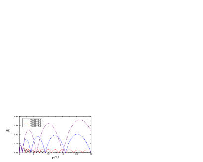
Figure 1: The phase diagram of superfluid-MI phase transition with different three-body interaction $W$.

The excitation spectrum and momentum distribution can be deduced from the second order action $S_{2}$. Introducing the Fourier transformation

$$\widetilde{a}(\vec{k},i\omega_{n})=\frac{1}{\sqrt{\beta N}}\int_{0}^{\beta}d\tau\sum_{i}\widetilde{a}_{i}(\tau)e^{-i\vec{k}\cdot\vec{R}_{i}+i\omega_{n}\tau},$$ (15)

where $N$ is the total number of lattice sites, $\vec{R}_{i}$ is a lattice vector for site $i$, $\omega_{n}=2n\pi/\beta$ is bosonic Matsubara frequency, $S_{2}$ becomes

$$S_{2} = \frac{1}{2}\sum_{\vec{k},\omega_{n}}\left[\widetilde{a}^{\ast}(\vec{k},i\omega_{n}),\widetilde{a}(-\vec{k},-i\omega_{n})\right]M_{2\times 2}\left[\widetilde{a}(\vec{k},i\omega_{n}),\widetilde{a}^{\ast}(-\vec{k},-i\omega_{n})\right]$$ (16)

with

$$M_{2\times 2} = \left(\begin{array}[]{cc}-G_{1c}^{-1}(i\omega_{n})+\varepsilon_{k}+2g\psi_{0}^{2}&g\psi_{0}^{2}\\ \\ g\psi_{0}^{2}&-G_{1c}^{-1}(-i\omega_{n})+\varepsilon_{-k}+2g\psi_{0}^{2}\end{array}\right)$$ (20)

and $\varepsilon_{k}=-2t(\cos{k_{x}}+\cos{k_{y}})$ denoting the boson dispersion in the absence of on-site interaction.

3.2 MI Phase

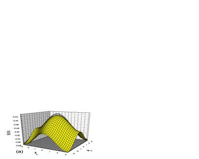
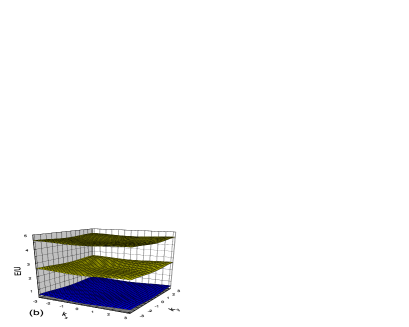
Figure 2: The excitation spectrum for quasiholes (a) and quasiparticles (b). We choose $t/U=0.01$, $\mu/U=1.5$ and $W/U=0,2.0,4.0$ to make the system into MI with the filling factor $n_{0}=2$. In (a) the effects of different $W$ is very small. In (b) from bottom to top $W$ is increasing.

In the MI phase $\psi_{0}=0$, the matrix $M_{2\times 2}$ becomes diagonal and $S_{2}$ is reduced into

$$S_{2}=\sum_{\vec{k},\omega_{n}}\widetilde{a}^{\ast}(\vec{k},i\omega_{n})\left[-G_{1c}^{-1}(i\omega_{n})+\varepsilon_{k}\right]\widetilde{a}(\vec{k},i\omega_{n}).$$ (21)

The Green function $g_{MI}(\vec{k},i\omega_{n})=-<\widetilde{a}(\vec{k},i\omega_{n})\widetilde{a}^{\ast}(\vec{k},i\omega_{n})>$ can be directly obtained $g_{MI}^{-1}(\vec{k},i\omega_{n})=G_{1c}^{-1}(i\omega_{n})-\varepsilon_{{k}}$. Using (10), we obtain

$$g_{MI}(\vec{k},i\omega_{n})=\frac{z_{k}}{i\omega_{n}-E_{k}^{+}}+\frac{1-z_{k}}{i\omega_{n}-E_{k}^{-}}$$ (22)

with

$$E_{k}^{\pm} = \frac{\epsilon_{n_{0}+1}-\epsilon_{n_{0}-1}+\varepsilon_{k}\pm\sqrt{\Delta_{k}}}{2},$$ (23)

$$\Delta_{k} = (\epsilon_{n_{0}+1}-\epsilon_{n_{0}-1}+\varepsilon_{k})^{2}-4(\epsilon_{n_{0}-1}-\epsilon_{n_{0}})(\epsilon_{n_{0}}-\epsilon_{n_{0}+1})$$ (24)

$$- 4\varepsilon_{k}[n_{0}(\epsilon_{n_{0}}-\epsilon_{n_{0}+1})+(n_{0}+1)(\epsilon_{n_{0}}-\epsilon_{n_{0}-1})],$$

$$z_{k} = \frac{E_{k}^{+}-n_{0}(\epsilon_{n_{0}}-\epsilon_{n_{0}+1})-(n_{0}+1)(\epsilon_{n_{0}}-\epsilon_{n_{0}-1})}{E_{k}^{+}-E_{k}^{-}}.$$ (25)

In (23), $E_{k}^{\mp}$ stand for excitations of quasiholes (removing particles from sites) or quasiparticles (adding particles to sites), which is consistent with the results in [17] and is shown in Fig.2(a) (Fig.2(b)). Very explicitly, three-body interaction $W$ has little impacts on quasihole excitations, but it has the large effects on quasiparticle excitation: with the increase of $W$, quasiparticle energy becomes higher, hence its excitation also becomes difficult.

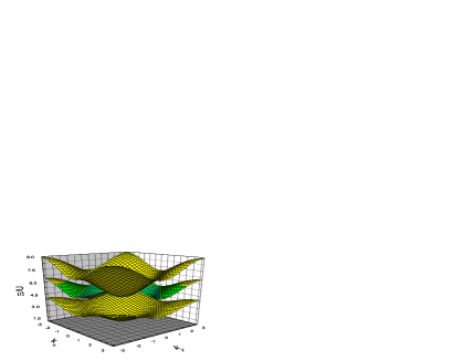
Figure 3: The excitation spectrum for density fluctuation $\Xi_{k}$. We choose $t/U=0.06$, $W/U=2.0$ and $\mu/U=1.5,5.5,10.5$ to make the system into MI with filling factor $n_{0}=2,3,4$ respectively. From bottom to top $\mu$ is increasing.

In Greiner’s experiment [1], Superfluid-MI phase transition is also detected by applying a potential gradient to the system in the MI phase and probing the excitation spectrum resulting from a particle-hole excitation. According to the above results, we can find a first approximation for the dispersion of particle-hole excitation (density fluctuations) $\Xi_{k}$ by subtracting $E_{k}^{-}$ from $E_{k}^{+}$, which yields

$$\Xi_{k}=E_{k}^{+}-E_{k}^{-}=\sqrt{\Delta_{k}}.$$ (26)

Due to little impacts of three-body interaction $W$ on $E_{k}^{-}$, the dependence of $\Xi_{k}$ on $W$ is the same as $E_{k}^{+}$. In Fig.3 we show $\Xi_{k}$ for a fixed $W$, but different filling factor $n_{0}$, i.e. different chemical potential $\mu$. We can see that in MI phases there is always a band gap increasing with the filling factor, which is different from the situation without three-body interaction where the gap is approximately independent of the filling factor. It is from this perspective that reference [20] proposed to observe weak three-body interaction for high filling MI.

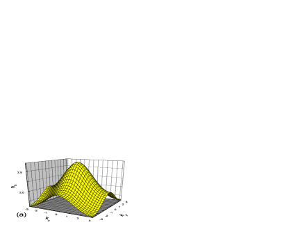
Figure 4: The momentum distribution in MI phases with filling factor $n_{0}=2.0$. Parameters are chosen as follows: $t/U=0.01$, $\mu/U=1.5$ and $W/U=0$ in (a) $W/U=2.0$ in (b).

From the theorem of fluctuation and dissipation, the momentum distribution at zero temperature $n_{k}=<\widetilde{a}^{\ast}(\vec{k})\widetilde{a}(\vec{k})>$ is

$$n_{k} = \int_{-\infty}^{\infty}\frac{d\omega}{2\pi}\frac{1}{e^{\beta\omega}-1}(-2)Im[g_{MI}(\vec{k},\omega+i0^{+})]$$ (27)

$$= \int_{-\infty}^{\infty}\frac{d\omega}{e^{\beta\omega}-1}[z_{k}\delta(\omega-E_{k}^{+})+(1-z_{k})\delta(\omega-E_{k}^{-})]=z_{k}-1,$$

where the label ”Im” denotes the imaginary part. In deriving (27) we have noted that quasiparticle dispersion $E_{k}^{+}$ is always greater than or equal to zero and $E_{k}^{-}$ is always smaller than or equal to zero. Because of this only the quasiholes give a contribution to the total density at zero temperature. Fig.4 shows momentum distributions in MI phases and we find that three-body interaction $W$ leads to not only flattening but also broadening of momentum distribution around $\vec{k}=0$.

3.3 Superfluid Phase

In terms of the superfluid phase, $\psi_{0}^{2}=(\overline{G}_{1c}^{-1}+4t)/g$. From the condition $det(M_{2\times 2})=0$, we obtain four excitation branches $\pm E_{k}^{\pm}$ with

$$E_{k}^{\pm 2} = -\frac{B_{k}}{2}\pm\frac{1}{2}(B_{k}^{2}-4C_{k})^{1/2},$$

$$B_{k} = 2h_{2}-2(\varepsilon_{k}+2g\psi_{0}^{2})h_{1}-(h_{3}-\varepsilon_{k}-2g\psi_{0}^{2})^{2}+g^{2}\psi_{0}^{4},$$

$$C_{k} = [h_{2}-(\varepsilon_{k}+2g\psi_{0}^{2})h_{1}]^{2}-g^{2}\psi_{0}^{4}h_{1}^{2},$$

$$h_{1} = (n_{0}+1)(\epsilon_{n_{0}-1}-\epsilon_{n_{0}})-n_{0}(\epsilon_{n_{0}}-\epsilon_{n_{0}+1}),$$

$$h_{2} = (\epsilon_{n_{0}-1}-\epsilon_{n_{0}})(\epsilon_{n_{0}}-\epsilon_{n_{0}+1}),$$

$$h_{3} = (\epsilon_{n_{0}-1}-\epsilon_{n_{0}})+(\epsilon_{n_{0}}-\epsilon_{n_{0}+1}).$$ (28)

Compared to the Bogoliubov’s theory for weakly interacting Bose gases, where only two excitation branches exist, there are two more excitation branches $\pm E_{k}^{+}$ due to renormalization of the tunneling term by locally exact single-particle Green function $\overline{G}_{1c}(i\omega)$. Fig.5 show typical characters for $E_{k}^{\pm}$: $E_{k}^{+}$ is gapped while $E_{k}^{-}$ is gapless. Moreover we also find that a gap opens between $E_{k}^{+}$ and $E_{k}^{-}$ when three-body interaction $W$ becomes strong. Here, we are only interested in gapless excitations described by $\pm E_{k}^{-}$, which originate from spontaneously broken gauge symmetry and describe the low energy behaviors of the system. By expanding $E_{k}^{-}$ in the vicinity of $\vec{k}=0$, we find a linear spectrum $E_{k}^{-}=vk$ with

$$v=\left[\frac{2t(\overline{G}_{1c}^{-1}+4t)}{\alpha^{2}+2\gamma(\overline{G}_{1c}^{-1}+4t)}\right]^{1/2},\alpha=\frac{h_{2}-h_{1}h_{3}}{h_{1}^{2}},\gamma=\frac{h_{1}^{2}+h_{2}-h_{1}h_{3}}{h_{1}^{3}}.$$ (29)

The existence of such linear spectrum is consistent with the Landau’s criterion of superfluidity [24]. Fig.6 shows the dependence of sound velocity $v$ on three-body interaction $W$. It is should be noted that the system is in the superfluid phase near $n_{0}=2$ MI phase for parameters $\mu$ and $t$ chosen in Fig.6. For different parameters $\mu$ and $t$, on the one hand $v$ generally is not monotonic as the function of $W$, on the other hand the critical values $W_{c}$, where $v=0$ or the system enters into the MI phase, are very different. The second character can be illustrated from the phase diagram Fig.1: with the increase of $W$, the left boundary of MI lobe with $n_{0}=2$ changes very slowly, but the right boundary changes very quickly.

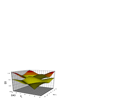
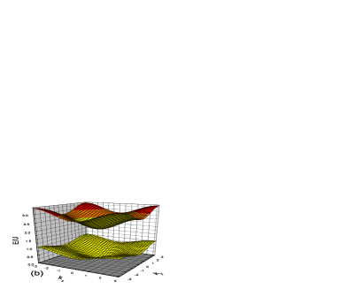
Figure 5: The excitation spectrum in superfluid phase with parameters $t/U=0.06$, $\mu/U=1.5$, $W/U=0.0$ in (a) and $W/U=2.0$ in (b).

From the excitation spectrum $\pm E_{k}^{\pm}$, the Green function $g_{SF}(\vec{k},i\omega_{n})$ can be easily obtained

$$g_{SF}(\vec{k},i\omega_{n})=\frac{P_{+}}{i\omega_{n}+E_{k}^{+}}+\frac{P_{-}}{i\omega_{n}-E_{k}^{+}}+\frac{Q_{+}}{i\omega_{n}+E_{k}^{-}}+\frac{Q_{-}}{i\omega_{n}-E_{k}^{-}},$$ (30)

where

$$P_{\pm} = \frac{E_{k}^{+3}\mp a_{2}E_{k}^{+2}-a_{1}E_{k}^{+}\mp a_{0}}{2E_{k}^{+}(E_{k}^{+2}-E_{k}^{-2})},Q_{\pm}=\frac{E_{k}^{-3}\mp a_{2}E_{k}^{-2}-a_{1}E_{k}^{-}\mp a_{0}}{2E_{k}^{-}(E_{k}^{-2}-E_{k}^{+2})},$$

$$a_{2} = h_{1}-h_{3}+\varepsilon_{k}+2g\psi_{0}^{2},a_{1}=h_{3}h_{1}-h_{2},a_{0}=h_{1}[h_{2}-h_{1}(\varepsilon_{k}+2g\psi_{0}^{2})].$$ (31)

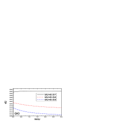
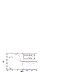
Figure 6: The sound velocity $v$ as the function of three-body interaction $W$ for (a) $\mu/U=1.2$, (b) $\mu/U=1.8$, (c) $t/U=0.06$.

Following the same steps in (27), the momentum distribution in the superfluid phase is

$$n_{k}=N\psi_{0}^{2}\delta_{k,0}-P_{+}-Q_{+},$$ (32)

where the first term $N\psi_{0}^{2}\delta_{k,0}$ comes from the condensate and it is this term that supplies a coherent peak in absorptive images of atom gases. Fig.7 show the momentum distribution from the second and third terms. In contrast to the situation in MI phases, three-body interaction $W$ only broadens the width of the peak near $\vec{k}=0$.

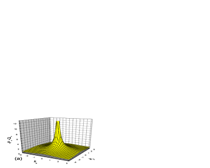
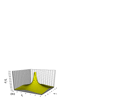
Figure 7: The momentum distribution in superfluid phase. Parameters are chosen as follows: $t/U=0.06$, $\mu/U=1.5$ and $W/U=0$ in (a) $W/U=2.0$ in (b).

4 Conclusions

In conclusion, an effective action for Bose-Hubbard model with two- and three-body on-site interaction in a square optical lattice has been derived by performing two successive Hubbard-Stratonovich transformations of the intersite hopping term. The main advantage of this method is that superfluid and MI phases can be analyzed on the same footing. Starting from this effective action, superfluid-MI phase transition, excitation spectrum and momentum distribution for two phases are calculated by taking into account Gaussian fluctuation about the saddle-point approximation. In addition the effects of three-body interaction are also discussed. We find that the sound velocity in superfluid phase generally is not monotonic as the function of three-body interaction, depending on the chemical potential and hopping term.

References

- [1] M. Greiner, O. Mandel, T. Esslinger, T. W. Hänsch and I. Bloch, Nature 415, 39 (2002).
- [2] M. P. A. Fisher, P. B. Weichmann, G. Grinstein and D. S. Fisher, Phys. Rev. B 40, 546 (1989).
- [3] D. Jaksch, C. Bruder, J. I. Cirac, C. W. Gardiner and P. Zoller, Phys. Rev. Lett. 81, 3108 (1998).
- [4] D. Jaksch, V. Venturi, J. I. Cirac, C. J. Williams and P. Zoller Phys. Rev. Lett. 89, 040402 (2002).
- [5] T. Köhler, Phys. Rev. Lett. 89, 210404 (2002).
- [6] P. R. Johnson, E. Tiesinga, J. V. Porto and C. J. Williams, New J. Phys. 11, 093022 (2009).
- [7] M. Greiner, O. Mandel, T. W. Häsch and I. Bloch, Nature 419, 51 (2002).
- [8] M. Anderlini, J. S. Strabley, J. Kruse, J. V. Porto and W. D. Phillips, J. Phys. B 39 S199 (2006).
- [9] J. S. Strabley, B. L. Brown, M. Anderlini, P. J. Lee, P. R. Johnson, W. D. Phillips and J. V. Porto, Phys. Rev. Lett. 98, 200405 (2007).
- [10] T. T. Wu, Phys. Rev. 115, 1390 (1959).
- [11] E. Braaten and A. Nieto, Eur. Phys. J. B 11, 143 (1999).
- [12] F. K. Abdullaev, A. Gammal, L. Tomio and T. Frederico, Phys. Rev. A 63, 043604 (2001).
- [13] S. T. Chui and V. N. Ryzhov, Phys. Rev. A 69, 043607 (2004).
- [14] D. Mozyrsky, I. Martin and E. Timmermans, Phys. Rev. A 76, 051601 (2007).
- [15] F. Ferlaino, C. D’Errico, G. Roati, M. Zaccanti, M. Inguscio, G. Modugno and A. Simoni, Phys. Rev. A 73, 040702 (2006).
- [16] C. A. Stan, M. W. Zwierlein, C. H. Schunck, S. M. F. Raupach and W. Ketterle, Phys. Rev. Lett. 93, 143001 (2004).
- [17] B. L. Chen, X. B. Huang, S. P. Kou and Y. Zhang, Phys. Rev. A 78, 043603 (2008).
- [18] B. Huang and S. Wan, Phys. Lett. A 374, 4364 (2010).
- [19] K. Zhou, Z. Liang and Z. Zhang, Phys. Rev. A 82, 013634 (2010).
- [20] M. Singh, A. Dhar, T. Mishra, R. V. Pai and B. P. Das, arXiv:1203.1412
- [21] K. Sengupta and N. Dupuis, Phys. Rev. A 71, 033629 (2005).
- [22] N. Dupuis, Nucl. Phys. B 618, 617 (2001).
- [23] J. W. Negele and H. Orland, Quantum Many Particles System (Addison-Wesley, Reading, MA, 1988).
- [24] L. D. Landau, J. Phys. (Moscow) 5, 71 (1941).