Stability of a force-based hybrid method with planar sharp interface

Abstract

We study a force-based hybrid method that couples atomistic model with Cauchy-Born elasticity model with sharp transition interface. We identify stability conditions that guarantee the convergence of the hybrid scheme to the solution of the atomistic model with second order accuracy, as the ratio between lattice parameter and the characteristic length scale of the deformation tends to zero. Convergence is established for hybrid schemes with planar sharp interface for system without defects, with general finite range atomistic potential and simple lattice structure. The key ingredient of the proof is regularity and stability analysis of elliptic systems of difference equations. We apply the results to atomistic-to-continuum scheme for a 2D triangular lattice with planar interface.

1 Introduction

Multiscale methods couple together atomistic and continuum models have received intense investigations in recent years; see, e.g., [TadmorOrtizPhillips:1996, AbBrBe98, E:book, TadmorMiller:book, LuskinOrtner]. Generally speaking, there are two main categories of methods coupling atomistic and continuum models: energy-based methods and force-based methods. The energy-based methods employ an energy that is a mixture of atomistic energy and continuum elastic energy. The energy functional is then minimized subject to suitable boundary conditions to obtain the deformed state of the system. The force-based methods work instead at the level of force balance equations. The forces derived from atomistic and continuum models are coupled together. The force balance equations supplemented with suitable boundary conditions are solved to obtain the deformed state of the system.

From a numerical analysis point of view, the key issue for these multiscale methods is the consistency and stability analysis of the coupled schemes [E:book]*Chapter 7. In this paper, we study force-based atomistic-to-continuum hybrid methods in two and three dimension with sharp transition between the atomistic and continuum regions. In our previous work [LuMing:2011], we developed the stability analysis in general dimension for a force-based atomistic-to-continuum method with smooth transition between the two regions. The main focus of the current paper is to extend the stability analysis of [LuMing:2011] to hybrid schemes with sharp interface between atomistic and continuum models.

Comprehensive reviews for force-based hybrid methods can be found in [MillerTadmor:2009]*Section 5 and Section 6 and [TadmorMiller:book]*Section 12.5. A class of force-based methods uses a handshake region (transition region) between the atomistic and continuum regions. A representative of such methods is the concurrent AtC coupling method (AtC) developed in a series of papers [BadiaBochvLehoucqParksFishNuggehallyGunzburger:2007, Fish:2007, Badia:2008, Parks:2008], which blends the continuum stress and the atomistic forces. The method recently proposed and analyzed by the authors in [LuMing:2011] shares certain common traits with the AtC method. It is proved to be stable and convergent with optimal convergence rate. The numerical implementation of the method can be found in [YangMingWu:2012].

As a representative for force-based methods without handshake region, the FEAt method of Kohlhoff, Gumbsch and Fischmeister [KohlhoffGumbschFischmeister:1991] is perhaps one of the earliest force-based methods. In this method, an elasticity model is coupled with an atomistic model. The FEAt method does not use a handshake region: the transition between the atomistic model and the continuum model is sharp. This kind of coupling is generalized in CADD method [ShilkrotMillerCurtin:2002], which uses the discrete dislocation model in the continuum region.

One of the main advantages of the force-based methods is that consistency is achieved with fairly simple construction. Hence the main focus of analyzing such methods is stability. The stability for one-dimensional force-based method was already understood in a series of nice works by Dobson, Luskin, Ortner, and Shapeev [DobsonLuskinOrtner:2010a, DobsonLuskinOrtner:2010b, DobsonOrtnerShapeev:12]. The generalization to higher dimension is nontrivial due to the complications of lattice structures and atomistic interaction potentials. The main idea in our previous paper [LuMing:2011] and the current paper is to establish linearized $H^{2}$-stability of the hybrid scheme by viewing the scheme as a nonlinear elliptic finite difference system and applying the elliptic regularity estimates to such system. The recent work [LiLuskinOrtner:12] by Li, Luskin and Ortner proved linearized $H^{1}$-stability for methods with smooth coupling under certain stability conditions. These conditions however were not yet known how to check explicitly. They also studied how the size of the transition region affects the stability.

For atomistic-to-continuum hybrid method with sharp interface studied in this paper, stability might fail at the interface. To make sure that the hybrid scheme is convergent, we need to check the stability conditions at the interface for the coupling schemes. We shall identify the interface stability conditions as analog of the complementing boundary conditions for elliptic PDE system. From a physical perspective, these stability conditions amount to check whether there exists nontrivial surface phonon at the interface of the two schemes. To some extent, these stability conditions are analogous to the famous Gustafsson-Kreiss-Sundström stability conditions [GKS:72] for finite difference approximations of mixed initial/boundary value problems.

The main result in this paper is the linearized $H^{2}$-stability and convergence of atomistic-to-continuum hybrid method under the stability conditions. The essential ingredients are regularity and stability analysis of finite difference schemes. As a consequence of our main results, we will show that a force-based atomistic-to-continuum coupling for a triangular lattice with next-nearest neighbor harmonic interaction is stable and hence convergent, when the interface between the atomistic and continuum regions is planar and is parallel to the $(1,\sqrt{3})/2$ direction of the lattice. Let us finally remark that while we focus on hybrid schemes coupling atomistic and nonlinear elasticity models, the ideas and techniques in the current paper can be extended to other force-based hybrid methods, e.g., the force-based coupling of peridynamics and nonlinear elasticity proposed in [SelesonaBeneddinebPrudhomme:2012].

1.1 Atomistic model and Cauchy-Born rule

We consider classical empirical potentials: For atoms located at $\{y_{1},\cdots,y_{K}\}$, the interaction potential energy between the atoms is given by $V(y_{1},\cdots,y_{K}),$ which often takes the form

$$V(y_{1},\cdots,y_{K})=\sum_{i,j}V_{2}(y_{i}/\varepsilon,y_{j}/\varepsilon)+\sum_{i,j,k}V_{3}(y_{i}/\varepsilon,y_{j}/\varepsilon,y_{k}/\varepsilon)+\cdots.$$

As in [EMing:2007] and our previous work [LuMing:2011], we make the following assumptions on the potential function $V$: $V$ is invariant with respect to translations and rigid body motion; $V$ is smooth in a neighborhood of the equilibrium state; and $V$ has finite range. For simplicity of notation and clarity of presentation, our presentation will be limited to potentials that contain only two-body and three-body potentials, and we will only make explicit the three-body terms in the expressions of the potential. As the potential function $V$ is a function of atom distances and angles by invariance with respect to rigid body motion, we may write

$$V_{3}(y_{i},y_{j},y_{k})=V_{3}\left(\left\lvert y_{i}-y_{j}\right\rvert^{2},\left\lvert y_{i}-y_{k}\right\rvert^{2},\left\langle y_{i}-y_{j},y_{i}-y_{k}\right\rangle\right),$$

where $\left\langle\cdot,\cdot\right\rangle$ denotes the inner product over $\mathbb{R}^{d}$.

We denote $\Omega_{\varepsilon}$ the collections of atom positions in equilibrium, with $x\in\Omega_{\varepsilon}$ denotes the equilibrium position of individual atom. Positions of the atoms under deformation will be viewed as a function defined over $\Omega_{\varepsilon}$, which is denoted as $y(x)=x+u(x)$. Hence, $u:\Omega_{\varepsilon}\to\mathbb{R}^{d}$ is the displacement of the atoms. We will use the same notations for lattice functions and theirs norms as in our previous work [LuMing:2011] (also recalled in the Supplementary Materials Section LABEL:sec:lattice for readers’ convenience). Define the space of the displacement field as

$$X_{\varepsilon}=\Bigl{\{}u:\Omega_{\varepsilon}\to\mathbb{R}^{d}\,\Big{|}\,\sum_{x\in\Omega_{\varepsilon}}u(x)=0\Bigr{\}}.$$

The atomistic problem is formulated as follows. Given force field $f_{\varepsilon}:\Omega_{\varepsilon}\to\mathbb{R}^{d}$, find $u\in X_{\varepsilon}$ such that

$$u=\arg\min_{u\in X_{\varepsilon}}I_{\and}(u),$$ (1)

where

$$I_{\and}(u)=\dfrac{1}{3!}\varepsilon^{d}\sum_{x\in\Omega_{\varepsilon}}\sum_{(s_{1},s_{2})\in S}V_{(s_{1},s_{2})}[x+u]-\varepsilon^{d}\sum_{x\in\Omega_{\varepsilon}}f_{\varepsilon}(x)u(x),$$

and

$$V_{(s_{1},s_{2})}[y]=V\left(\left\lvert D_{\varepsilon,s_{1}}^{+}y(x)\right\rvert^{2},\left\lvert D_{\varepsilon,s_{2}}^{+}y(x)\right\rvert^{2},\left\langle D_{\varepsilon,s_{1}}^{+}y(x),D_{\varepsilon,s_{2}}^{+}y(x)\right\rangle\right).$$

Here $S$ is the set of all possible $(s_{1},s_{2})$ within the range of the potential. By our assumptions, $S$ is a finite set. In $I_{\and}$, $\varepsilon^{d}$ is a normalization factor, so that $I_{\and}$ is actually the energy of the system per atom.

The Euler-Lagrange equation for the atomistic problem is

$$\mathcal{F}_{\and}[u](x)=f_{\varepsilon}(x)\qquad x\in\Omega_{\varepsilon},$$ (2)

where

$$\mathcal{F}_{\and}[u](x) =\sum_{(s_{1},s_{2})\in S}\Bigl{(}D_{\varepsilon,s_{1}}^{-}\left(2\partial_{1}V_{(s_{1},s_{2})}[y](x)D_{\varepsilon,s_{1}}^{+}y(x)+\partial_{3}V_{(s_{1},s_{2})}[y](x)D_{\varepsilon,s_{2}}^{+}y(x)\right)$$

$$\phantom{\sum_{(s_{1},s_{2})}}\qquad+D_{\varepsilon,s_{2}}^{-}\left(2\partial_{2}V_{(s_{1},s_{2})}[y](x)D_{\varepsilon,s_{2}}^{+}y(x)+\partial_{3}V_{(s_{1},s_{2})}[y](x)D_{\varepsilon,s_{1}}^{+}y(x)\right)\Bigr{)},$$

where for $i=1,2,3$, we denote

$$\partial_{i}V_{(s_{1},s_{2})}[y](x)=\partial_{i}V\left(\left\lvert D_{\varepsilon,s_{1}}^{+}y(x)\right\rvert^{2},\left\lvert D_{\varepsilon,s_{2}}^{+}y(x)\right\rvert^{2},\left\langle D_{\varepsilon,s_{1}}^{+}y(x),D_{\varepsilon,s_{2}}^{+}y(x)\right\rangle\right)$$

the partial derivative with respect to the $i$-th argument of $V$.

To guarantee the solvability of (2), we assume that $f_{\varepsilon}$ takes the following form:

$$f_{\varepsilon}(x)\equiv\varepsilon^{-d}\int_{x+\varepsilon\Gamma}f(z)\,\mathrm{d}z,\quad x\in\Omega_{\varepsilon},$$

where $f(x)$ is a function defined on $\Omega$ with zero mean. This makes sure that $f_{\varepsilon}(x)$ satisfies

$$\sum_{x\in\Omega_{\varepsilon}}f_{\varepsilon}(x)=\varepsilon^{-d}\int_{\Omega}f(x)\,\mathrm{d}x=0.$$

To introduce the Cauchy-Born elasticity problem [BornHuang:1954, Ericksen:1984, Ericksen:2008], we fix more notations. For any positive integer $k$, we denote by $W^{k,p}(\Omega;\mathbb{R}^{d})$ the Sobolev space of mappings $u{:}\;\Omega\to\mathbb{R}^{d}$ such that $\|u\|_{W^{k,p}}$ is finite, and by $W_{\#}^{k,p}(\Omega;\mathbb{R}^{d})$ the Sobolev space of periodic functions whose distributional derivatives of order less than $k$ are in $L^{p}(\Omega)$. For any $p>d$ and $m\geq 0$, we define $X$ as

$$X=\Bigl{\{}u:\Omega\to\mathbb{R}^{d}\,\Big{|}\,u\in W^{m+2,p}(\Omega;\mathbb{R}^{d})\cap\,W_{\#}^{1,p}(\Omega;\mathbb{R}^{d}),\,\int_{\Omega}u=0\Bigr{\}}.$$

The Cauchy-Born elasticity problem is formulated as follows. Find $u\in X$ such that

$$u=\arg\min_{u\in X}I(u),$$ (3)

where the total energy functional $I$ is given by

$$I(u)=\int_{\Omega}\bigl{(}W_{\mathrm{CB}}(\nabla u(x))-f(x)u(x)\bigr{)}\,\mathrm{d}x.$$

Here the Cauchy-Born stored energy density $W_{\mathrm{CB}}$ is given by

$$W_{\mathrm{CB}}(A)=\dfrac{1}{3!}\sum_{(s_{1},s_{2})\in S}W_{(s_{1},s_{2})}(A),$$

where for $A\in\mathbb{R}^{d\times d}$,

$$W_{(s_{1},s_{2})}(A)=V\left(\left\lvert s_{1}+s_{1}A\right\rvert^{2},\left\lvert s_{2}+s_{2}A\right\rvert^{2},\left\langle s_{1}+s_{1}A,s_{2}+s_{2}A\right\rangle\right).$$

The range $S$ is the same as that in the atomistic potential function.

The Euler-Lagrange equation for the Cauchy-Born elasticity model is

$$\mathcal{F}_{\mathrm{CB}}[u](x)=f(x),$$ (4)

where $\mathcal{F}_{\mathrm{CB}}[u]=-\operatorname{div}\bigl{(}D_{A}W_{\mathrm{CB}}(\nabla u)\bigr{)}$ with $D_{A}W_{\mathrm{CB}}(A)$ denoting the derivative of $W_{\mathrm{CB}}(A)$ with respect to $A$. Since we are primarily interested in the coupling between the atomistic and continuum models, we will take the finite element mesh $\mathcal{T}_{\varepsilon}$ as a triangulation of $\Omega_{\varepsilon}$ with each atom site as an element vertex. The triangulation is translational invariant. The approximation space $\widetilde{X}_{\varepsilon}$ is defined as

$$\widetilde{X}_{\varepsilon}=\bigl{\{}u\in W^{1,p}_{\#}(\Omega;\mathbb{R}^{d})\mid u|_{T}\in P_{1}(T),\ \forall\,T\in\mathcal{T}_{\varepsilon}\bigr{\}},$$

where $P_{1}(T)$ is the space of linear functions on the element $T$. We denote by $\mathcal{F}_{\varepsilon}$ the force from finite element approximation of Cauchy-Born elasticity problem (3).

1.2 Formulation of force-based hybrid method with sharp interface

To formulate the force-based hybrid method, we take a continuum region

$$\Omega_{c}=\Bigl{\{}\sum_{j=1}^{d}x_{j}a_{j}\,\Big{|}\,0\leq x_{1}<1/2,\,0\leq x_{j}<1,\,j=2,\cdots,d\Bigr{\}},$$

and denote $\varrho$ the characteristic function associated with $\Omega_{c}$: $\varrho(x)=1$ if $x\in\Omega_{c}$. $\Omega_{a}=\Omega\backslash\Omega_{c}=\{x\mid\varrho(x)=0\}$ is the atomistic region. The continuum region and atomistic region are separated by two hyperplanes $\{x_{1}=0\}$ and $\{x_{1}=1/2\}$ as a result of periodic boundary condition. The simple geometry here is chosen for simplicity of presentation. Using localization techniques as in [LaxNirenberg:1966], we may generalize the analysis to any $\Omega_{c}$ with smooth boundary.

We consider a force field defined by

$$\mathcal{F}_{\mathrm{hy}}[u](x)\equiv\bigl{(}1-\varrho(x)\bigr{)}\mathcal{F}_{\and}[u](x)+\varrho(x)\mathcal{F}_{\varepsilon}[u](x),\qquad x\in\Omega_{\varepsilon}.$$ (5)

Due to the choice of $\varrho$, in the atomistic region $\Omega_{a}$, the force acting on the atom is just that of atomistic model, while in the continuum region $\Omega_{c}$, the force is calculated from finite element approximation of the Cauchy-Born elasticity. Since $\varrho$ is taken to be the characteristic function, we consider here a hybrid method with sharp interface, i.e., there is no transition or buffer region between the atomistic and continuum regions.

Given a loading $f_{\varepsilon}$, we find $u\in X_{\varepsilon}$ such that

$$(\Pi_{\varepsilon}\mathcal{F}_{\mathrm{hy}}[u])(x)=f_{\varepsilon}(x)\qquad x\in\Omega_{\varepsilon},$$ (6)

where for a lattice function $g$, $\Pi_{\varepsilon}$ projects $g$ to a function with zero mean.

$$(\Pi_{\varepsilon}g)(x){:}=g(x)-\varepsilon^{d}\sum_{x^{\prime}\in\Omega_{\varepsilon}}g(x^{\prime}).$$

As in [LuMing:2011], the convergence of the hybrid scheme is tightly connected with its linear stability. Thus, it is natural to study the linearized operator of $\mathcal{F}_{\mathrm{hy}}$. Denote $\mathcal{H}_{\mathrm{hy}}[u]$ the linearization of $\mathcal{F}_{\mathrm{hy}}$ at state $u$: $\mathcal{H}_{\mathrm{hy}}[u]=\delta\mathcal{F}_{\mathrm{hy}}/\delta u$, so that $\mathcal{H}_{\mathrm{hy}}[u]$ is a linear operator acting on a lattice functions $w$, which is given by

$$\mathcal{H}_{\mathrm{hy}}[u]w=\lim_{t\to 0}\dfrac{\partial\mathcal{F}_{\mathrm{hy}}}{\partial t}[u+tw].$$

We will rewrite the operator $\mathcal{H}_{\mathrm{hy}}$ in the form of a difference operator as

$$\mathcal{H}_{\mathrm{hy}}[u]=\sum_{\mu\in\mathcal{A}}h_{\mathrm{hy}}[u](x,\mu)T^{\mu},$$

where the coefficient $h_{\mathrm{hy}}[u](x,\mu)$ is a $d$ by $d$ matrix (probably asymmetric) for each $x\in\Omega_{\varepsilon}$ and $\mu\in\mathcal{A}$, which is given by

$$(h_{\mathrm{hy}}[u])_{\alpha\beta}(x,\mu)=\frac{\partial(\mathcal{F}_{\mathrm{hy}}[u])_{\alpha}(x)}{\partial(T^{\mu}u)_{\beta}(x)},\quad\alpha,\beta=1,\cdots,d.$$ (7)

Here $\mathcal{A}$ is the stencil of the difference operator, which is finite by assumptions on the atomistic potential. By the definition of $\mathcal{F}_{\mathrm{hy}}$, we have

$$h_{\mathrm{hy}}[u](x,\mu)=\bigl{(}1-\varrho(x)\bigr{)}h_{\and}[u](x,\mu)+\varrho(x)h_{\varepsilon}[u](x,\mu),$$ (8)

where $h_{\and}[u]$ and $h_{\varepsilon}[u]$ are given by similar equations as (7) with $\mathcal{F}_{\mathrm{hy}}$ replaced by $\mathcal{F}_{\and}$ and $\mathcal{F}_{\varepsilon}$, respectively.

Define $h_{\mathrm{hy}}[u](x,\xi)$ as the symbol of the pseudo-difference operator $\mathcal{H}_{\mathrm{hy}}[u]$, which is given by

$$h_{\mathrm{hy}}[u](x,\xi)=\sum_{\mu\in\mathcal{A}}h_{\mathrm{hy}}[u](x,\mu)\exp\Bigl{(}\imath\varepsilon\sum_{j}\mu_{j}a_{j}\cdot\xi\Bigr{)}\qquad\text{for }\xi\in\mathbb{L}^{\ast}_{\varepsilon},$$

and similarly for $h_{\varepsilon}[u]$ and $h_{\and}[u]$. By definition, we have for any $x\in\Omega_{\varepsilon}$,

$$(\mathcal{H}_{\mathrm{hy}}[u]e_{k}e^{\imath x\cdot\xi})_{j}(x)=(h_{\mathrm{hy}}[u])_{jk}(x,\xi)e^{\imath x\cdot\xi},$$

for $j,k=1,\dots,d$ and similarly for $h_{\varepsilon}[u]$ and $h_{\and}[u]$. It is also clear that (8) implies

$$h_{\mathrm{hy}}[u](x,\xi)=(1-\varrho(x))h_{\and}[u](x,\xi)+\varrho(x)h_{\varepsilon}[u](x,\xi).$$ (9)

When $\mathcal{F}_{\mathrm{hy}}$ is linearized around the equilibrium state $u=0$, we will simplify the notation as $\mathcal{H}_{\mathrm{hy}}=\mathcal{H}_{\mathrm{hy}}[0]$, $h_{\mathrm{hy}}=h_{\mathrm{hy}}[0]$, and similarly for those defined for atomistic model and finite element discretization of the Cauchy-Born elasticity. By the translation invariance of the total energy $I_{\and}$ at the state $u=0$, we observe that the coefficients of the symbols $h_{\and}(x,\mu)$ and $h_{\varepsilon}(x,\mu)$ are independent of the position $x$, i.e.,

$$h_{\and}(x,\mu)=h_{\and}(\mu),\quad h_{\varepsilon}(x,\mu)=h_{\varepsilon}(\mu).$$

We also denote $\mathcal{H}_{\mathrm{CB}}$ as the linearization of $\mathcal{F}_{\mathrm{CB}}$ at the equilibrium state $u=0$, and define $h_{\mathrm{CB}}(x,\xi)$ as its symbol. Due to the periodic boundary condition, the argument $\xi$ in the symbol $h_{\mathrm{CB}}(x,\xi)$ only takes value in $\mathbb{L}^{\ast}$. Again, due to the translation invariance of the total energy, the symbol $h_{\mathrm{CB}}$ is also independent of $x$.

An elementary calculation shows that the matrices $h_{\and}(\xi)$, $h_{\varepsilon}(\xi)$ and hence $h_{\mathrm{hy}}(x,\xi)$ are Hermitian for any $\varepsilon>0$. As in [LuMing:2011], we make the following stability assumption on the atomistic potential:

Assumption A.

The matrix $h_{\and}(\xi)$ is positive definite and there exists a positive constant $a_{\and}$ such that for any $\varepsilon>0$ and any $\xi\in\mathbb{L}_{\varepsilon}^{\ast}$,

$$\det{h}_{\and}(\xi)\geq a_{\and}\Lambda_{0,\varepsilon}^{2d}(\xi).$$

1.3 Stability conditions at the interface

The main focus of the current paper is to establish convergence for the hybrid method with sharp interface as $\varepsilon\to 0$. In [LuMing:2011], convergence was proved for any short-range interaction potentials when $\varrho$ is a smooth function, or in other words, when the transition region between atomistic and continuum regions is of $\mathcal{O}(\varepsilon^{-1})$. In this paper, as the transition is sharp, we require additional stability conditions to guarantee convergence.

To understand better where the additional stability assumptions come from, let us reformulate the hybrid scheme as a system of difference equations with boundary conditions by folding with respect to the interface (similar folding trick was used in [Ciment:1971]). This is one of the keys to establish the stability for the hybrid scheme. Let us consider domain

$$\Omega_{\mathrm{strip}}=\Bigl{\{}xa_{1}+\sum_{j}y_{j}a_{j+1}\mid x\in\mathbb{R},\,y\in[0,1)^{d-1}\Bigr{\}}$$

with periodic boundary condition in $y$ variable. $\Omega_{\mathrm{strip}}$ is discretized by grid points $(x_{\nu},y_{\mu})$ with $x_{\nu}=\varepsilon\nu a_{1}$ with $\nu\in\mathbb{Z}$ and $y_{\mu}=\varepsilon\sum_{j}\mu_{j}a_{j+1}$ with $\mu\in\mathbb{Z}^{d-1}$. We consider the following hybrid system on $\Omega_{\mathrm{strip}}$:

$$\sum_{j=1}^{d}(\mathcal{H}_{\varepsilon,ij}u_{j})(x_{\nu},y_{\mu})=f_{i}(x_{\nu},y_{\mu}), \nu<0,\ i=1,\cdots,d;$$ (10)

$$\sum_{j=1}^{d}(\mathcal{H}_{\and,ij}u_{j})(x_{\nu},y_{\mu})=f_{i}(x_{\nu},y_{\mu}), \nu\geq 0,\ i=1,\cdots,d.$$ (11)

As we will see later, the stability analysis of the coupled system is the key to understand the stability of the hybrid scheme with sharp interface.

Let $(\underline{\nu}^{c}_{ij},\overline{\nu}^{c}_{ij})$ and $(\underline{\nu}^{a}_{ij},\overline{\nu}^{a}_{ij})$ be the extent of the stencils of $\mathcal{H}_{\varepsilon,ij}$ and $\mathcal{H}_{\and,ij}$ in $x$ direction respectively. To simplify the presentation, we will assume that the extents are the same for all $i,j$’s, which is usually the case for applications in atomistic-continuum hybrid schemes. We denote them as $(\underline{\nu}^{c},\overline{\nu}^{c})$ and $(\underline{\nu}^{a},\overline{\nu}^{a})$. The construction can be extended to more general cases, which will be omitted for simplicity. Without loss of generality, we also assume that $\underline{\nu}^{a}\leq\underline{\nu}^{c}\leq 0\leq\overline{\nu}^{c}\leq\overline{\nu}^{a}$.

To do the folding, we rename the variables as

$$U_{i}(x_{\nu},y_{\mu})=u_{i}(x_{\overline{\nu}^{c}-\nu-1},y_{\mu}), \nu\geq 0,\mu\in\mathbb{R}^{d-1};$$

$$U_{d+i}(x_{\nu},y_{\mu})=u_{i}(x_{\underline{\nu}^{a}+\nu},y_{\mu}), \nu\geq 0,\mu\in\mathbb{R}^{d-1}.$$

This leads to $d(\overline{\nu}^{c}-\underline{\nu}^{a})$ compatibility conditions

$$U_{i}(x_{\nu},y_{\mu})=U_{d+i}(x_{\overline{\nu}^{c}-\underline{\nu}^{a}-\nu-1},y_{\mu}),\quad 0\leq\nu\leq\overline{\nu}^{c}-\underline{\nu}^{a}-1,\,i=1,\cdots,d.$$ (12)

We will rewrite equations (10)-(11) in terms of $U$’s. Define

$$L_{\varepsilon,ij}=\begin{cases}\displaystyle\sum_{0\leq\nu\leq\overline{\nu}^{c}-\underline{\nu}^{c},\mu}h_{\varepsilon,ij}(\overline{\nu}^{c}-\nu,\,\mu)T_{\varepsilon,x}^{\nu}T_{\varepsilon,y}^{\mu},&i,j=1,\cdots,d;\\ \displaystyle\sum_{\underline{\nu}^{a}\leq\nu\leq\overline{\nu}^{a},\,\mu}h_{\and,(i-d)(j-d)}(\nu,\mu)T_{\varepsilon,x}^{\nu}T_{\varepsilon,y}^{\mu},&i,j=d+1,\cdots,2d;\\ 0,&\text{otherwise.}\end{cases}$$

By construction, the extents of the operators $L_{\varepsilon}$ are given by

$$(\underline{\nu}_{ij},\overline{\nu}_{ij})=\begin{cases}(0,\overline{\nu}^{c}-\underline{\nu}^{c}),&i,j=1,\cdots,d;\\ (0,\overline{\nu}^{a}-\underline{\nu}^{a}),&i,j=d+1,\cdots,2d;\\ (0,0),&\text{otherwise.}\end{cases}$$

Let

$$F_{i}(x_{\nu},y_{\mu})=\begin{cases}f_{i}(x_{-\nu-1},y_{\mu}),&i=1,\cdots,d;\\ f_{i-d}(x_{\nu},y_{\mu}),&i=d+1,\cdots,2d,\end{cases}$$

we then have

$$\sum_{j=1}^{2d}(L_{\varepsilon,ij}U_{j})(x_{\nu},y_{\mu})=F_{i}(x_{\nu},y_{\mu}),\qquad\nu\geq 0,\mu\in\mathbb{Z}^{d-1}.$$ (13)

We further define for $k=1,\cdots,d(\overline{\nu}^{c}-\underline{\nu}^{a})$ and $j=1,\cdots,d$,

$$B_{\varepsilon,kj}=(D_{\varepsilon,e_{1}}^{+})^{i}I\delta_{jl},\qquad B_{\varepsilon,k(j+d)}=-(D_{\varepsilon,-e_{1}}^{+})^{i}T_{\varepsilon,x}^{\overline{\nu}^{c}-\underline{\nu}^{a}-1}\delta_{jl},$$

where $i=\lfloor(k-1)/d\rfloor$ and $l=[(k-1)\mod d]+1$. The compatibility conditions (12) are then equivalent to the boundary conditions

$$\sum_{j=1}^{2d}(B_{\varepsilon,kj}U_{j})(x_{0},y_{\mu})=0,\qquad\mu\in\mathbb{Z}^{d-1},k=1,\cdots,d(\overline{\nu}^{c}-\underline{\nu}^{a}).$$ (14)

Therefore, we have reformulated (10)-(11) into a difference system (13) with boundary conditions (14).

We now state the additional stability conditions, which can be understood as conditions to make sure that the solutions to the finite difference system is regular up to the boundary. Taking $\alpha^{+}=0$, $\beta_{j}^{+}=\overline{\nu}^{c}-\underline{\nu}^{c}$, $j=1,\cdots,d$, and $\beta_{j}^{+}=\overline{\nu}^{a}-\underline{\nu}^{a}$, $j=d+1,\cdots,2d$, we have then $0\leq\underline{\nu}_{ij}\leq\overline{\nu}_{ij}\leq\alpha_{i}^{+}+\beta_{j}^{+}$. The number of boundary conditions we have imposed on (14) is $q=d(\overline{\nu}^{c}-\underline{\nu}^{a})$.

Assumption B.

The number of boundary conditions $d(\overline{\nu}^{c}-\underline{\nu}^{a})$ is equal to the total number of roots of

$$R^{c}(z,\eta)=\det\left[h_{\varepsilon,ij}(-i\varepsilon^{-1}\log z,\varepsilon^{-1}\eta)\right]=0;$$

$$R^{a}(z,\eta)=\det\left[h_{\and,ij}(-i\varepsilon^{-1}\log z,\varepsilon^{-1}\eta)\right]=0.$$

satisfying $0<\left\lvert z(\eta)\right\rvert<1$ for $\left\lvert\eta\right\rvert\neq 0$.

The stability of the hybrid scheme relies on the stability at interface, which is characterized by the complementing boundary condition.

Assumption C.

The hybrid system (10)-(11), or equivalently (13)-(14) satisfies the Complementing Boundary Condition, defined below in Section 2.3.

The complementing boundary conditions are natural analog of corresponding complementing boundary conditions for continuous elliptic system, as in [AgmonDouglisNirenberg:1959], which will be explained in details in Section 2.3. This stability assumption needs to be checked for particular atomic interaction potentials. Examples can be found in Section 4.

1.4 Main result

The main result of this paper is

Theorem 1 (Convergence).

Under Assumptions A, B, and C, there exist positive constants $\delta$ and $M$, so that for any $p>d$ and $f\in W^{15,p}(\Omega)\cap W^{1,p}_{\#}(\Omega)$ with $\left\lVert f\right\rVert_{W^{15,p}}\leq\delta$, we have $\left\lVert y_{\mathrm{hy}}-y_{\and}\right\rVert_{\varepsilon,2}\leq M\varepsilon^{2}$.

Remark. The Assumption A is a natural stability condition for the atomistic lattice system. Compared with the convergence result in [LuMing:2011], the additional assumptions B and C come from the coupling between the atomistic potential and the finite element discretization at the interface.

The proof of Theorem 1 follows a similar strategy as in [LuMing:2011]. Actually, once we obtain the stability estimate Theorem 9, the proof of Theorem 1 is essentially the same as that of [LuMing:2011]*Theorem 1.1. The consistency analysis of the scheme follows from that of [LuMing:2011]*Section 2 with some immediate adaptations. Observe in particular that the proof of consistency does not depend on the smoothness of $\varrho$. Hence, we will focus on the linear stability analysis, and omit the consistency part.

The remaining of the paper is organized as follows. In Section 2, we recall the regularity theory for elliptic difference system with boundary conditions and use it to establish the regularity estimates for the hybrid scheme. The stability estimate then follows from the regularity estimate combined with consistency, which is presented in Section 3. In Section 4, we apply the general theory to two examples of force-based atomistic-to-continuum hybrid method for $2D$ triangular lattice with next-nearest neighbor harmonic interaction and truncated Lennard-Jones potential. We make some conclusive remarks in Section 5.

2 Regularity estimate of hybrid schemes

To analyze the general hybrid scheme, we will take the viewpoint of our previous work [LuMing:2011] and regard the scheme as a nonlinear finite difference scheme. One of the main ingredients we will use in this paper is the regularity estimates up to the boundary for elliptic difference systems established in [StrikwerdaWadeBube:1990]. We also note that the regularity estimates of elliptic difference equations and systems have been investigated by several works [LaxNirenberg:1966, ThomeeWestergren:1968, Hackbusch:1981, Hackbusch:1983, BubeStrikwerda:1983, StrikwerdaWadeBube:1990, Martin:94]. For reader’s convenience, we recall here briefly the setup and results with some adaptation to the current work.

2.1 Difference operators

We write a difference operator $L_{\varepsilon}$ in the form of

$$(L_{\varepsilon}u)(x)=\sum_{\mu\in\mathcal{A}}l_{\varepsilon}(x,\mu)(T^{\mu}_{\varepsilon}u)(x),$$ (15)

where the stencil $\mathcal{A}\subset\mathbb{Z}^{d}$ is finite. We define the symbol of $L_{\varepsilon}$ as

$$l_{\varepsilon}(x,\zeta)=\sum_{\mu\in\mathcal{A}}l_{\varepsilon}(x,\mu)e^{\imath 2\pi\varepsilon\mu\cdot\zeta}$$ (16)

for any $\zeta\in\mathbb{Z}^{d}$. By definition, we have

$$\Bigl{(}L_{\varepsilon}e^{\imath x\cdot(\zeta_{j}b_{j})}\Bigr{)}(x)=l_{\varepsilon}(x,\zeta)e^{\imath x\cdot(\zeta_{j}b_{j})}.$$

We choose $\mathcal{A}$ as the minimal stencil, that is, for $\mu\in\mathcal{A}$, the symbol $l_{\varepsilon}(x,\mu)$ is not identically zero. For this choice of $\mathcal{A}$, we let

$$\underline{\mu}_{i}=\min_{\mu\in\mathcal{A}}\mu_{i},\quad\overline{\mu}_{i}=\max_{\mu\in\mathcal{A}}\mu_{i},\qquad i=1,\cdots,d,$$

and call $(\underline{\mu}_{i},\overline{\mu}_{i})$ the extent of the difference operator in $x_{i}$ direction.

2.2 Elliptic difference system

Consider a half-space

$$\Omega_{\mathrm{half}}=\Bigl{\{}xa_{1}+\sum_{j}y_{j}a_{j+1}\mid x\geq 0,y\in[0,1)^{d-1}\Bigr{\}}$$

with periodic boundary condition in $y$. $\Omega_{\mathrm{half}}$ is discretized by grid points $(x_{\nu},y_{\mu})$ with mesh size $\varepsilon=1/(2N)$. Here $x_{\nu}=\varepsilon\nu a_{1}$ with $\nu\geq 0$ and $y_{\mu}=\varepsilon\sum_{j}\mu_{j}a_{j+1}$ with $\mu\in\mathbb{Z}^{d-1}$. Consider a linear system of difference equations with boundary conditions

$$\sum_{j=1}^{n}(L_{\varepsilon,ij}u_{j})(x_{\nu},y_{\mu})=f_{i}(x_{\nu},y_{\mu}),\qquad i=1,\cdots,n$$ (17)

$$\sum_{j=1}^{n}(B_{\varepsilon,kj}u_{j})(x_{0},y_{\mu})=0,\qquad k=1,\cdots,q.$$ (18)

We denote $l_{\varepsilon,ij}$ the symbol of $L_{\varepsilon,ij}$ and $b_{\varepsilon,kj}$ the symbol of $B_{\varepsilon,kj}$ viewed as difference operators on the whole space, defined as in (16). For our purpose, it suffices to consider the case that the coefficients of difference operators are independent of $x$, $y$, and $\varepsilon$, i.e.,

$$l_{\varepsilon,ij}(x,y,\nu,\mu)=l_{ij}(\nu,\mu),\qquad b_{\varepsilon,kj}(y,\nu,\mu)=b_{kj}(\nu,\mu).$$

We will henceforth make this simplification. Note that the symbols $l_{\varepsilon,ij}$ and $b_{\varepsilon,kj}$ however still depend on $\varepsilon$.

Definition 2 (Regular elliptic difference system).

We call (17) a regular elliptic of order $(\sigma,\tau)$ for $\sigma,\tau\in\mathbb{Z}^{n}$ if the following conditions are satisfied.

1. For each $i,j=1,\cdots,n$ and $\varepsilon$ sufficiently small, $\left\lvert l_{\varepsilon,ij}(\zeta)\right\rvert\lesssim\Lambda_{\varepsilon}(\zeta)^{\sigma_{i}+\tau_{j}}$;

2. There exist positive constants $\zeta_{0}$ and $\varepsilon_{0}$ such that $\left\lvert\det l_{\varepsilon}(\zeta)\right\rvert\gtrsim\Lambda_{\varepsilon}(\zeta)^{2p}$ for all $0<\varepsilon\leq\varepsilon_{0}$ and $\left\lvert\zeta\right\rvert\geq\zeta_{0}$, where $2p=\sum_{i}(\sigma_{i}+\tau_{i})$.

As a convention, we will choose $\sigma$ and $\tau$ so that $\max\sigma_{i}=0$. We also take $\rho\in\mathbb{Z}^{q}$ so that $\left\lvert b_{\varepsilon,kj}(\zeta)\right\rvert\lesssim\Lambda_{\varepsilon}(\zeta)^{\rho_{k}+\tau_{j}}$, with $\rho_{k}$ is the smallest possible integer such that the estimate hold. $(\rho,\tau)$ gives the order of $B_{\varepsilon}$ viewing as difference operators on the whole space. We will assume that the operators $L_{\varepsilon,ij}$ and $B_{\varepsilon,kj}$ only contain differences of order $\sigma_{i}+\tau_{j}$ and $\rho_{k}+\tau_{j}$, respectively.

Assumption 1.

Let the difference operators $L_{\varepsilon,ij}$ have extent $(\underline{\nu}_{ij},\overline{\nu}_{ij})$ in $x-$direction, we assume that there are $\alpha^{+},\beta^{+}$ in $\mathbb{Z}^{d}$ such that

$$0\leq\underline{\nu}_{ij}\leq\overline{\nu}_{ij}\leq\alpha_{i}^{+}+\beta_{j}^{+},\qquad i,j=1,\cdots,n,$$

and such that the number of roots $z(\eta)$, counting multiplicity, of the equation $R(z,\eta)=0$ is $\sum_{i}(\alpha_{i}^{+}+\beta_{i}^{+})$. Here

$$R(z,\eta)=\det\biggl{[}\sum_{\nu\in\mathbb{Z}}\sum_{\mu\in\mathbb{Z}^{d-1}}l_{ij}(\nu,\mu)z^{\nu}e^{\imath\mu\cdot\eta}\biggr{]}=\det\bigl{[}l_{\varepsilon,ij}(-\imath\varepsilon^{-1}\log z,\varepsilon^{-1}\eta)\bigr{]}.$$

Furthermore, the number of boundary conditions $q$ is equal to the number of roots of $R(z,\eta)=0$ that satisfy $0<\left\lvert z(\eta)\right\rvert<1$ for $\left\lvert\eta\right\rvert\neq 0$.

When $q$ is larger than $p$, an additional assumption is needed. We assume that the boundary conditions are ordered so that $\rho_{k}$ are in increasing order. We define

$$\widebar{\rho}=\max_{1\leq k\leq p}(\rho_{k}+1,0),\quad\text{and}\quad\rho^{\ast}=\begin{cases}\displaystyle\min_{k>p}\rho_{k}+1,&\text{if }q>p\,;\\ \infty,&\text{if }q=p\,.\end{cases}$$

Assumption 2.

The boundary operators satisfy $\rho_{k}\geq\widebar{\rho}$ for $p<k\leq q$.

In the limit $\varepsilon\to 0$, we obtain the system of differential equations associated with the system of difference equations.

$$\sum_{j=1}^{n}(L_{ij}(\partial_{x},\partial_{y})u_{j})(x,y)=f_{i}(x,y) i=1,\cdots,n,$$

$$\sum_{j=1}^{n}(B_{kj}(\partial_{x},\partial_{y})u_{j})(0,y)=0 k=1,\cdots,p.$$

The symbol of $L_{ij}$ is given by $l_{ij}(\zeta)=\lim_{\varepsilon\to 0}l_{\varepsilon,ij}(\zeta)$.

Assumption 3 (Supplementary condition).

The determinant $\det[l_{ij}(\zeta)]$ is of even degree $2p$. For every pair of vectors $\zeta,\zeta^{\prime}\in\mathbb{R}^{d}$, the polynomial $\det[l_{ij}(\zeta+\tau\zeta^{\prime})]$ in the complex variable $\tau$ has exactly $p$ roots with positive imaginary part.

2.3 Complementing boundary condition

Due to periodicity in $y$, we may reduce the system to a one dimensional operator by Fourier transform. Let $G$ be the tangential grid given by $G=\bigl{\{}y_{\mu}\mid 0\leq\mu_{j}<2N,j=1,\cdots,d-1\bigr{\}}$. The discrete Fourier transform for lattice functions $u$ with respect to $y$ is then

$$\widehat{u}(x_{\nu},\eta)=\Bigl{(}\frac{\varepsilon}{2\pi}\Bigr{)}^{d-1}\sum_{y_{\mu}\in G}e^{-\imath 2\pi\varepsilon\eta\cdot\mu}u(x_{\nu},y_{\mu}),$$

for $\eta\in\mathbb{Z}^{d-1}$ with $\left\lvert\eta_{j}\right\rvert\leq N$ for $j=1,\cdots,d-1$. The reduced operator is given by

$$\widetilde{L}_{\varepsilon,ij}(\eta)=\sum_{\nu\in\mathbb{Z}}\widetilde{l}_{\varepsilon,ij}(\nu,\eta)T^{\nu}_{\varepsilon},$$

where the coefficients $\widetilde{l}_{\varepsilon,ij}$ for $\eta\in\mathbb{Z}^{d-1}$ are given by $\widetilde{l}_{\varepsilon,ij}(\nu,\eta)=\sum_{\mu}l_{ij}(\nu,\mu)e^{\imath 2\pi\varepsilon\mu\cdot\eta}$. Analogously, we define $\widetilde{B}_{\varepsilon,kj}$ as the reduced operator of $B_{\varepsilon,kj}$. We denote $\widetilde{B}^{1}_{\varepsilon}$ the operators corresponding to the first $p$ boundary conditions and $\widetilde{B}^{2}_{\varepsilon}$ for the remaining $q-p$ ones. Similarly, we also denote the reduced operators for $L_{ij}$ as

$$\widetilde{L}_{ij}(\partial_{x},\theta)=L_{ij}(\partial_{x},\imath\theta),\qquad\text{for }\theta\in S^{d},$$

and analogously for $B_{kj}$. For these reduced operators, we consider three types of eigensolutions, which are defined as follows.

Definition 3.

We call an eigensolution of type I a nontrivial solution of

$$(\widetilde{L}_{\varepsilon}(\eta)w)(x_{\nu})=0\qquad\text{for some }\eta\neq 0,$$

satisfying (a) $(\widetilde{B}^{1}_{\varepsilon}(\eta)w)(x_{0})=0$; (b) $(\widetilde{B}^{2}_{\varepsilon}(\eta)w)(x_{0})=0$; (c) $w(x_{\nu})\to 0\ \text{as}\ \nu\to\infty$.

Definition 4.

We call an eigensolution of type II a nontrivial solution of

$$(\widetilde{L}(\partial_{x},\theta)w)(x)=0\qquad\text{for some }\theta\in S^{d},$$

satisfying (a) $(\widetilde{B}^{1}(\partial_{x},\theta)w)(x_{0})=0$; (b) $w(x)\to 0\ \text{as}\ x\to\infty$.

Definition 5.

We call an eigensolution of type III a nontrivial solution to

$$(\widetilde{L}_{\varepsilon}(0)w)(x)=0,$$

satisfying (a) $(\widetilde{B}^{2}_{\varepsilon}(0)w)(x_{0})=0$; (b) $w(x_{\nu})\to 0\ \text{as}\ \nu\to\infty$.

Remark. We remark that type I and type III eigensolutions are connected to the notion of surface phonon in the physics literature. The complementing conditions give a mathematical characterization of the surface phonon. On the other hand, the type II eigensolutions are surface waves at the boundary of the PDE.

Definition 6 (Complementing Boundary Condition).

The system (17) with boundary conditions (18) satisfies the Complementing Boundary Condition if there are no eigensolutions of type I, II, or III.

We state the following regularity estimate of the solution of elliptic system with boundary conditions, which is an adaptation of [StrikwerdaWadeBube:1990]*Theorem 3.1 to our setting.

Theorem 7.

If $u$ is a solution to the system (17) with boundary conditions (18) and Assumptions 1, 2, and 3 are satisfied, then the following regularity estimate holds for each $s$ with $\widebar{\rho}\leq s<\rho^{\ast}$ and $\varepsilon$ sufficiently small, if and only if, the Complementing Boundary Condition holds.

$$\left\lVert u\right\rVert_{\varepsilon,\tau+s}^{2}\lesssim\left\lVert f\right\rVert_{\varepsilon,s-\sigma}^{2}+\left\lVert u\right\rVert_{\varepsilon,0}^{2},$$

2.4 Regularity estimate for hybrid schemes

We will prove the regularity estimate for the the linearized operator $\mathcal{H}_{\mathrm{hy}}=\mathcal{H}_{\mathrm{hy}}[0]$ of the hybrid scheme by applying the regularity estimate Theorem 7.

Theorem 8 (Regularity).

Under Assumptions A, B, and C, for any $v\in H^{2}_{\varepsilon}(\Omega)$, we have for $\varepsilon$ sufficiently small

$$\left\lVert v\right\rVert_{\varepsilon,2}\lesssim\left\lVert\mathcal{H}_{\mathrm{hy}}v\right\rVert_{\varepsilon,0}+\left\lVert v\right\rVert_{\varepsilon,0}.$$ (19)

Proof.

By a standard localization argument as in [LaxNirenberg:1966], it suffices to show that for a solution $u$ of the system (10)-(11), the following regularity estimate holds for $\varepsilon$ sufficiently small

$$\left\lVert u\right\rVert_{\varepsilon,2}\lesssim\left\lVert f\right\rVert_{\varepsilon,0}+\left\lVert u\right\rVert_{\varepsilon,0}.$$ (20)

Recall that after folding with respect to the interface, the system (10)-(11) is equivalent to the system (13) with boundary conditions (14). Let us now verify that the system (13)-(14) satisfies the assumptions of Theorem 7. First by construction of the operator $L$, we know that

$$\det l_{\varepsilon,ij}(\zeta)=\det h_{\varepsilon,ij}(\zeta)\det h_{\and,ij}(\zeta).$$ (21)

The regular ellipticity of the operator $L_{\varepsilon}$ is guaranteed by Assumption A, as $\mathcal{H}_{\and}$ and $\mathcal{H}_{\varepsilon}$ are both regular elliptic by [LuMing:2011, Lemma 3.3]. Moreover, the order of $L_{\varepsilon}$ is $(2,0)$, and hence, $p=2d$. From (21), the Assumption 1 for the system (13)-(14) is equivalent to Assumption B. By definition, we have

$$\rho_{k}=\lfloor(k-1)/d\rfloor-2.$$

Hence, $\overline{\rho}=0$ and $\rho^{\ast}=1$. Assumption 2 is also satisfied by the system (13)-(14). The Supplementary Assumption 3 is automatically satisfied since $2d\geq 3$ as a result in [AgmonDouglisNirenberg:1959].

Applying Theorem 7, we have $\left\lVert U\right\rVert_{\varepsilon,2}\lesssim\left\lVert F\right\rVert_{\varepsilon,0}+\left\lVert U\right\rVert_{\varepsilon,0}$. By definition of $F$ and $U$, it is clear that $\left\lVert F\right\rVert_{\varepsilon,0}=\left\lVert f\right\rVert_{\varepsilon,0}$, $\left\lVert U\right\rVert_{\varepsilon,0}\leq 2\left\lVert u\right\rVert_{\varepsilon,0}$, and $\left\lVert u\right\rVert_{\varepsilon,2}\leq\left\lVert U\right\rVert_{\varepsilon,2}$. Therefore, we arrive at the desired estimate (20). ∎

3 Stability

The main purpose of this section is to establish the following stability estimate.

Theorem 9 (Stability).

Under Assumptions A, B, and C, for any $v\in H^{2}_{\varepsilon}(\Omega)$ with mean zero, we have

$$\left\lVert v\right\rVert_{\varepsilon,2}\lesssim\left\lVert\mathcal{H}_{\mathrm{hy}}v\right\rVert_{\varepsilon,0}$$ (22)

for $\varepsilon$ sufficiently small.

To obtain the stability estimate from the regularity estimate Theorem 8, we need to eliminate $\left\lVert v\right\rVert_{\varepsilon,0}$ on the right hand side of (19). The proof is based on the uniqueness of the continuous system from ellipticity, the consistency of the finite difference schemes to the continuous system, and the regularity estimate Theorem 8. We remark that the stability analysis in our previous work [LuMing:2011] relies on the smoothness of $\varrho$, so it does not apply to the sharp transition case. The current proof does not require smoothness of $\varrho$ and so applies both to the hybrid method with smooth or sharp transitions.

In order to connect the finite difference system with continuous PDE, we need to extend grid functions on $\Omega_{\varepsilon}$ to continuous functions defined in $\Omega$. For this purpose, let us define an interpolation operator $Q_{\varepsilon}$ as follows. For any lattice function $u$ on $\Omega_{\varepsilon}$, we define $Q_{\varepsilon}u\in L^{2}(\Omega)$ as

$$(Q_{\varepsilon}u)(x)=\sum_{\xi\in\mathbb{L}_{\varepsilon}^{\ast}}e^{\imath x\cdot\xi}\widehat{u}(\xi),\quad x\in\Omega.$$ (23)

By the Fourier inversion formula, we know that $Q_{\varepsilon}u$ agrees with $u$ on $\Omega_{\varepsilon}$. We recall that by [LuMing:2011]*Lemma 4.2,

$$c_{k}\left\lVert u\right\rVert_{H^{k}_{\varepsilon}(\Omega)}\leq\left\lVert Q_{\varepsilon}u\right\rVert_{H^{k}(\Omega)}\leq C_{k}\left\lVert u\right\rVert_{H^{k}_{\varepsilon}(\Omega)},\quad\forall\;k\geq 0.$$ (24)

Let $\chi$ be a standard nonnegative cut-off function on $\mathbb{R}^{d}$, which is smooth and compactly supported, with $\left\lVert\chi\right\rVert_{L^{1}}=1$. Let $\chi_{\varepsilon}$ be the scaled version $\chi_{\varepsilon}(x)=\varepsilon^{-(\alpha d)}\chi(\varepsilon^{-\alpha}x)$ for some $\alpha$ with $0<\alpha<1$. The choice of the value of $\alpha$ will be specified in the proof of Proposition 11. Define a low-pass filter operator $K_{\varepsilon}$ for $f\in L^{2}(\Omega)$ using $\widehat{\chi_{\varepsilon}}$ as Fourier multiplier:

$$\widehat{K_{\varepsilon}f}(\xi)=(2\pi)^{d}\widehat{f}(\xi)\widehat{\chi_{\varepsilon}}(\xi)=(2\pi)^{d}\widehat{f}(\xi)\widehat{\chi}(\varepsilon^{\alpha}\xi).$$

In real space, $K_{\varepsilon}$ convolves $f$ with $\chi_{\varepsilon}$. Integrating by parts, we obtain

$$\left\lvert\widehat{\chi_{\varepsilon}}(\xi)\right\rvert\leq C_{k}\left\lvert\varepsilon^{\alpha}\xi\right\rvert^{-k}\quad\text{for all}\ k\in\mathbb{Z}_{+},$$ (25)

$$(2\pi)^{d}\widehat{\chi_{\varepsilon}}(0)=1.$$ (26)

Hence, $K_{\varepsilon}$ is indeed a low-pass filter. For simplicity of notation, we denote

$$\widebar{u}_{\varepsilon}=K_{\varepsilon}Q_{\varepsilon}u_{\varepsilon}$$

for any lattice function $u_{\varepsilon}$ on $\Omega_{\varepsilon}$.

We will use the following result on the consistency of the symbols. It is an easy corollary from the consistency of the scheme, the details can be found in the Supplementary Materials Section LABEL:sec:cons.

Lemma 10 (Consistency of symbols of linearized operators).

There exists $\varepsilon_{0}>0$ and $s>0$ such that for any $\varepsilon\leq\varepsilon_{0}$, $x\in\Omega_{\varepsilon}$, and $\xi\in\mathbb{L}^{\ast}_{\varepsilon}$, we have

$$\left\lvert{h}_{\and}(\xi)-{h}_{\mathrm{CB}}(\xi)\right\rvert\leq C\varepsilon^{2}(1+\left\lvert\xi\right\rvert^{2})^{s/2},$$ (27)

$$\left\lvert{h}_{\and}(\xi)-{h}_{\mathrm{hy}}(x,\xi)\right\rvert\leq C\varepsilon^{2}(1+\left\lvert\xi\right\rvert^{2})^{s/2}.$$ (28)

The key element of the proof of Theorem 9 is the following proposition.

Proposition 11.

For $\{v_{\varepsilon}\}_{\varepsilon>0}$ such that $v_{\varepsilon}\in H^{2}_{\varepsilon}(\Omega)$ and $\left\lVert v_{\varepsilon}\right\rVert_{\varepsilon,2}$ is uniformly bounded, we have $\lim_{\varepsilon\to 0+}\left\lVert\mathcal{H}_{\mathrm{CB}}\widebar{v}_{\varepsilon}-\widebar{\mathcal{H}_{\mathrm{hy}}v_{\varepsilon}}\right\rVert_{L^{2}(\Omega)}=0$.

Proof.

By triangular inequality,

$$\left\lVert\mathcal{H}_{\mathrm{CB}}\widebar{v}_{\varepsilon}-\widebar{\mathcal{H}_{\mathrm{hy}}v_{\varepsilon}}\right\rVert_{L^{2}(\Omega)}\leq\left\lVert\overline{\mathcal{H}_{\mathrm{hy}}\widebar{v}_{\varepsilon}}-\widebar{\mathcal{H}_{\mathrm{hy}}v_{\varepsilon}}\right\rVert_{L^{2}(\Omega)}+\left\lVert\overline{\mathcal{H}_{\and}\widebar{v}_{\varepsilon}}-\overline{\mathcal{H}_{\mathrm{hy}}\widebar{v}_{\varepsilon}}\right\rVert_{L^{2}(\Omega)}\\ +\left\lVert\mathcal{H}_{\mathrm{CB}}\widebar{v}_{\varepsilon}-\overline{\mathcal{H}_{\and}\widebar{v}_{\varepsilon}}\right\rVert_{L^{2}(\Omega)}.$$

Hence, it suffices to show each term on the right-hand side goes to zero as $\varepsilon\to 0$.

Step 1. By (24) and the definition of $\mathcal{H}_{\mathrm{hy}}$, we have

$$\left\lVert\overline{\mathcal{H}_{\mathrm{hy}}\widebar{v}_{\varepsilon}}-\widebar{\mathcal{H}_{\mathrm{hy}}v_{\varepsilon}}\right\rVert_{L^{2}(\Omega)} \leq\left\lVert\mathcal{H}_{\mathrm{hy}}\widebar{v}_{\varepsilon}-\mathcal{H}_{\mathrm{hy}}v_{\varepsilon}\right\rVert_{\varepsilon,0}$$

$$\leq\left\lVert\mathcal{H}_{\and}\widebar{v}_{\varepsilon}-\mathcal{H}_{\and}v_{\varepsilon}\right\rVert_{\varepsilon,0}+\left\lVert\mathcal{H}_{\varepsilon}\widebar{v}_{\varepsilon}-\mathcal{H}_{\varepsilon}v_{\varepsilon}\right\rVert_{\varepsilon,0}.$$

We now show that $\left\lVert\mathcal{H}_{\varepsilon}\widebar{v}_{\varepsilon}-\mathcal{H}_{\varepsilon}v_{\varepsilon}\right\rVert_{\varepsilon,0}$ converges to zero as $\varepsilon\to 0$, the argument for the other term is identical. By Parseval’s identity,

$$\left\lVert\mathcal{H}_{\varepsilon}\widebar{v}_{\varepsilon}-\mathcal{H}_{\varepsilon}v_{\varepsilon}\right\rVert_{\varepsilon,0}=\left\lVert{h}_{\varepsilon}(\xi)(\widehat{\chi_{\varepsilon}}(\xi)-1)\widehat{v}_{\varepsilon}(\xi)\right\rVert_{l^{2}(\mathbb{L}_{\varepsilon}^{\ast})}.$$ (29)

Note that $\left\lVert{h}_{\varepsilon}(\xi)\widehat{v}_{\varepsilon}(\xi)\right\rVert_{l^{2}(\mathbb{L}_{\varepsilon}^{\ast})}=\left\lVert\mathcal{H}_{\varepsilon}v_{\varepsilon}\right\rVert_{\varepsilon,0}$ is bounded as $v_{\varepsilon}\in H^{2}_{\varepsilon}(\Omega)$ and that $\widehat{\chi_{\varepsilon}}(\xi)\to 1$ for any $\xi\in\mathbb{L}_{\varepsilon}^{\ast}$, as $\varepsilon\to 0$. By dominance convergence, the right-hand side of (29) converges to zero in the limit. Therefore, $\left\lVert\overline{\mathcal{H}_{\mathrm{hy}}\widebar{v}_{\varepsilon}}-\widebar{\mathcal{H}_{\mathrm{hy}}v_{\varepsilon}}\right\rVert_{L^{2}(\Omega)}\to 0$.

Step 2. By (24), we have

$$\left\lVert\overline{\mathcal{H}_{\and}\widebar{v}_{\varepsilon}}-\overline{\mathcal{H}_{\mathrm{hy}}\widebar{v}_{\varepsilon}}\right\rVert_{L^{2}(\Omega)}\lesssim\left\lVert\mathcal{H}_{\and}\widebar{v}_{\varepsilon}-\mathcal{H}_{\mathrm{hy}}\widebar{v}_{\varepsilon}\right\rVert_{\varepsilon,0}.$$

Hence it suffices to estimate the right-hand side. We calculate

$$\mathcal{H}_{\and}\widebar{v}_{\varepsilon}-\mathcal{H}_{\mathrm{hy}}\widebar{v}_{\varepsilon}=\sum_{\xi\in\mathbb{L}_{\varepsilon}^{\ast}}({h}_{\and}(\xi)-{h}_{\mathrm{hy}}(x,\xi))\widehat{\widebar{v}}_{\varepsilon}(\xi)e^{\imath x\cdot\xi}.$$

Therefore, using (28) in Lemma 10, we have

$$\left\lVert\mathcal{H}_{\and}\widebar{v}_{\varepsilon}-\mathcal{H}_{\mathrm{hy}}\widebar{v}_{\varepsilon}\right\rVert_{\varepsilon,0}^{2}\lesssim\sum_{\xi\in\mathbb{L}_{\varepsilon}^{\ast}}\varepsilon^{4}(1+\left\lvert\xi\right\rvert^{2})^{s}{\bigl{|}\widehat{\widebar{v}}_{\varepsilon}(\xi)\bigr{|}}^{2}.$$

To estimate the right-hand side, note that by (25) we have for any $k\in\mathbb{Z}_{+}$,

$$\left\lvert\widehat{\widebar{v}}_{\varepsilon}(\xi)\right\rvert^{2}=\left\lvert\widehat{\chi_{\varepsilon}}(\xi)\right\rvert^{2}\left\lvert\widehat{v}_{\varepsilon}(\xi)\right\rvert^{2}\leq C_{k}\left\lvert\varepsilon^{\alpha}\xi\right\rvert^{-2k}\left\lvert\widehat{v}_{\varepsilon}(\xi)\right\rvert^{2}.$$

Taking $k$ sufficiently large so that $(1+\left\lvert\xi\right\rvert^{2})^{s}\left\lvert\xi\right\rvert^{-2k}$ is bounded for $\xi\in\mathbb{L}^{\ast}\backslash\{0\}$, we then have

$$\left\lVert\mathcal{H}_{\and}\widebar{v}_{\varepsilon}-\mathcal{H}_{\mathrm{hy}}\widebar{v}_{\varepsilon}\right\rVert_{\varepsilon,0}^{2}\lesssim\varepsilon^{4}\varepsilon^{-2\alpha k}\sum_{\xi\in\mathbb{L}_{\varepsilon}^{\ast}}\left\lvert\widehat{v}_{\varepsilon}(\xi)\right\rvert^{2}.$$

Choose $\alpha$ in the low-pass filter such that $\alpha<2/k$, we get $\left\lVert\overline{\mathcal{H}_{\and}\widebar{v}_{\varepsilon}}-\overline{\mathcal{H}_{\mathrm{hy}}\widebar{v}_{\varepsilon}}\right\rVert_{L^{2}(\Omega)}\to 0$ as $\varepsilon\to 0+$.

Step 3. By definition, $\widehat{\mathcal{H}_{\mathrm{CB}}\widebar{v}_{\varepsilon}}(\xi)={h}_{\mathrm{CB}}(\xi)\widehat{\chi}(\varepsilon^{\alpha}\xi)\widehat{v}_{\varepsilon}(\xi)$. For the discrete system, we have

$$\widehat{\widebar{\mathcal{H}_{\and}v_{\varepsilon}}}(\xi) =\widehat{\chi}(\varepsilon^{\alpha}\xi)\Bigl{(}\frac{\varepsilon}{2\pi}\Bigr{)}^{d}\sum_{x\in\Omega_{\varepsilon}}e^{-\imath\xi\cdot x}\sum_{\eta\in\mathbb{L}^{\ast}_{\varepsilon}}e^{\imath x\cdot\eta}{h}_{\and}(\eta)\widehat{v}_{\varepsilon}(\eta)$$

$$=\widehat{\chi}(\varepsilon^{\alpha}\xi){h}_{\and}(\xi)\widehat{v_{\varepsilon}}(\xi).$$

Hence, we have, combined with (27) and (25), for some $s>0$ and any $k\in\mathbb{Z}_{+}$,

$$\left\lVert\mathcal{H}_{\mathrm{CB}}\widebar{v}_{\varepsilon}-\widebar{\mathcal{H}_{\and}v_{\varepsilon}}\right\rVert_{L^{2}(\Omega)}^{2} =\sum_{\xi\in\mathbb{L}_{\varepsilon}^{\ast}}({h}_{\and}(\xi)-{h}_{\mathrm{CB}}(\xi))^{2}\left\lvert\widehat{\chi}(\varepsilon^{\alpha}\xi)\right\rvert^{2}\left\lvert\widehat{v}_{\varepsilon}(\xi)\right\rvert^{2}$$

$$\leq C_{k}\varepsilon^{4}\sum_{\xi\in\mathbb{L}_{\varepsilon}^{\ast}}(1+\left\lvert\xi\right\rvert)^{s}\left\lvert\varepsilon^{\alpha}\xi\right\rvert^{-2k}\left\lvert\widehat{v}_{\varepsilon}(\xi)\right\rvert^{2}.$$

We choose a sufficiently large $k$, so that the right-hand side is bounded by $C\varepsilon^{4-2\alpha k}\left\lVert v_{\varepsilon}\right\rVert_{\varepsilon,0}^{2}$. The choice of $\alpha<2/k$ as above guarantees that $\left\lVert\mathcal{H}_{\mathrm{CB}}\widebar{v}_{\varepsilon}-\widebar{\mathcal{H}_{\and}v_{\varepsilon}}\right\rVert_{L^{2}(\Omega)}\to 0$ as $\varepsilon\to 0$. ∎

Proof of Theorem 9.

Suppose (22) does not hold, then there is a sequence of functions $\{w_{k}\}$ and $\varepsilon_{k}>0$ such that $\lim_{k\to\infty}\left\lVert w_{k}\right\rVert_{\varepsilon_{k},2}\to\infty$, and $\left\lVert\mathcal{H}_{\mathrm{hy}}w_{k}\right\rVert_{\varepsilon_{k},0}\leq c$ and $\sum_{x\in\Omega_{\varepsilon_{k}}}w_{k}(x)=0$ for all $k$. Set $v_{k}=w_{k}/\left\lVert w_{k}\right\rVert_{\varepsilon_{k},2}$, we then have

$$\left\lVert v_{k}\right\rVert_{\varepsilon_{k},2}=1\quad\text{and}\quad\sum_{x\in\Omega_{\varepsilon_{k}}}v_{k}(x)=0\qquad\text{for all }k;\qquad\lim_{k\to\infty}\left\lVert\mathcal{H}_{\mathrm{hy}}v_{k}\right\rVert_{\varepsilon_{k},0}\to 0.$$

Note that $\mathcal{H}_{\mathrm{CB}}\widebar{v}_{k}=\widebar{\mathcal{H}_{\mathrm{hy}}v_{k}}+(\mathcal{H}_{\mathrm{CB}}\widebar{v}_{k}-\widebar{\mathcal{H}_{\mathrm{hy}}v_{k}})$. Since $\left\lVert\mathcal{H}_{\mathrm{hy}}v_{k}\right\rVert_{\varepsilon_{k},0}\to 0$, we have $\left\lVert\widebar{\mathcal{H}_{\mathrm{hy}}v_{k}}\right\rVert_{L^{2}(\Omega)}\to 0$, as $k\to\infty$. Moreover, by Proposition 11,

$$\left\lVert\mathcal{H}_{\mathrm{CB}}\widebar{v}_{k}-\widebar{\mathcal{H}_{\mathrm{hy}}v_{k}}\right\rVert_{L^{2}(\Omega)}\to 0\quad\text{as }k\to\infty.$$

Hence $\left\lVert\mathcal{H}_{\mathrm{CB}}\widebar{v}_{k}\right\rVert_{L^{2}(\Omega)}\to 0$. Note also that the average of $\widebar{v}_{k}$ is zero, since $\widehat{\widebar{v}_{k}}(0)=0$. By the invertibility of $\mathcal{H}_{\mathrm{CB}}$ on the subspace orthogonal to constant function, $\left\lVert\widebar{v}_{k}\right\rVert_{L^{2}(\Omega)}\to 0$, as $k\to\infty$, while $\left\lVert v_{k}\right\rVert_{\varepsilon_{k},2}=1$. It follows then $\left\lVert v_{k}\right\rVert_{\varepsilon_{k},0}\to 0$. Indeed, since

$$\left\lVert v_{k}\right\rVert_{\varepsilon_{k},1}=\sum_{\xi\in\mathbb{L}^{\ast}_{\varepsilon_{k}}}\Lambda^{2}_{\varepsilon_{k}}(\xi)\left\lvert\widehat{v}_{k}(\xi)\right\rvert^{2}\leq 1,$$

for any $\delta>0$, there exist $\Xi>0$ and $k_{1}$, such that for any $k\geq k_{1}$,

$$\sum_{\xi\in\mathbb{L}^{\ast}_{\varepsilon_{k}},\,\left\lvert\xi\right\rvert\geq\Xi}\left\lvert\widehat{v}_{k}(\xi)\right\rvert^{2}<\delta/2.$$ (30)

On the other hand, due to (26), there exists $k_{2}$, such that for $k\geq k_{2}$

$$\sum_{\xi\in\mathbb{L}^{\ast}_{\varepsilon_{k}},\,\left\lvert\xi\right\rvert<\Xi}\Bigl{\lvert}\left\lvert\widehat{v}_{k}(\xi)^{2}\right\rvert-\left\lvert\widehat{\widebar{v}}_{k}(\xi)\right\rvert^{2}\Bigr{\rvert}\leq\delta/4.$$ (31)

Moreover, as $\left\lVert\widebar{v}_{k}\right\rVert_{L^{2}}\to 0$, there exists $k_{3}$, such that for $k\geq k_{3}$,

$$\sum_{\xi\in\mathbb{L}^{\ast}_{\varepsilon_{k}},\left\lvert\xi\right\rvert<\Xi}\left\lvert\widehat{\widebar{v}}_{k}(\xi)\right\rvert^{2}\leq\delta/4.$$ (32)

Combining (30)–(32) together, we have for $k\geq\max(k_{1},k_{2},k_{3})$,

$$\left\lVert v_{k}\right\rVert_{\varepsilon_{k},0}^{2}=\sum_{\xi\in\mathbb{L}^{\ast}_{\varepsilon_{k}}}\left\lvert\widehat{v}_{k}\right\rvert^{2}\leq\delta.$$

Hence, $\lim_{k\to\infty}\left\lVert v_{k}\right\rVert_{\varepsilon_{k},0}=0$. From Theorem 8, this implies $\lim_{k\to\infty}\left\lVert v_{k}\right\rVert_{\varepsilon_{k},2}=0$. The contradiction with the choice of $v_{k}$ proves the Theorem. ∎

4 Example

We apply the result here to some concrete examples of atomistic-to-continuum hybrid method. More specifically, we check the assumptions of Theorem 9 which then imply the stability of the scheme near the ground state.

4.1 Example 1. Triangular lattice with harmonic interaction

Consider a force-based method on a triangular lattice. Figure 1 gives the geometry and the choice of the atomistic and continuum regions. The interface between the atomistic and continuum regions is parallel to the $(1,\sqrt{3})/2$ direction of the lattice. The interaction between atoms is assumed to be harmonic (quadratic potential). The force balance equation reads

$$\Pi_{\varepsilon}\mathcal{F}_{\mathrm{hy}}[z](x)=f_{\varepsilon}(x),$$ (33)

with $\mathcal{F}_{\mathrm{hy}}$ given by $\mathcal{F}_{\and}$ in $\Omega_{a}$ and by $\mathcal{F}_{\varepsilon}$ in $\Omega_{c}$, where

$$\mathcal{F}_{\and}[z](x){:}=\dfrac{1}{\varepsilon}\sum_{i=1}^{12}D_{\varepsilon,\mu_{i}}^{+}z(x),\qquad\mathcal{F}_{\varepsilon}[z](x){:}=\dfrac{4}{\varepsilon}\sum_{i=1}^{6}D_{\varepsilon,\mu_{i}}^{+}z(x),$$

where $\{\mu_{i}\}_{i=1}^{6}$ and $\{\mu_{i}\}_{i=7}^{12}$ are the first and the second neighborhood interaction ranges of the triangular lattice $\mathbb{L}$, respectively.

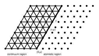
Fig. 1: Illustration of the geometry of the hybrid method. The coordinate of each atom is $(\nu,\mu)$, and the interface $\Gamma$ along the atoms labeled with $(0,\mu)$. The interface $\Gamma$ divides the domain into the atomistic region $\Omega_{a}$ and the continuum region $\Omega_{c}$.

We rewrite the coupled force balance equation into a system. For any $x=ma_{1}+na_{2}\in\Omega_{a}$, we define the map $\widetilde{x}=-ma_{1}+na_{2}$, and denote $z(x)=\bigl{(}y(x-2a_{1}),y(\widetilde{x})\bigr{)}$, where $a_{1}$ and $a_{2}$ are the basis vectors of the triangular lattice $\mathbb{L}$. The hybrid method can be rewritten as

$$\mathcal{F}_{\mathrm{hy}}[z](x)=\ell_{\varepsilon}(x),$$ (34)

where $\mathcal{F}_{\mathrm{hy}}=\bigl{(}\begin{smallmatrix}\mathcal{F}_{\and}&0\\ 0&\mathcal{F}_{\varepsilon}\end{smallmatrix}\bigr{)}$ and $\ell_{\varepsilon}(x)=\bigl{(}f_{\varepsilon}(x-2a_{1}),f_{\varepsilon}(\widetilde{x})\bigr{)}$. It is supplemented with the following boundary conditions:

$$\sum_{j=1}^{2}B_{\varepsilon,kj}z_{j}(x)=0,\qquad x\in\Gamma,k=1,2,3,$$ (35)

where $B_{\varepsilon,k1}=\left(D_{\varepsilon,\mu_{1}}^{+}\right)^{k-1}$, and $B_{\varepsilon,k2}=-\left(D_{\varepsilon,\mu_{1}}^{+}\right)^{k-1}T_{\varepsilon}^{-2\mu_{1}}$.

Applying Fourier transform in the tangential direction $a_{2}$, we obtain

$$\widetilde{\mathcal{F}}_{\varepsilon} =\dfrac{4}{\varepsilon^{2}}\left(T_{\varepsilon}^{\mu_{1}}(1+e^{-\imath\xi\cdot\mu_{2}})+T_{\varepsilon}^{-\mu_{1}}(1+e^{\imath\xi\cdot\mu_{2}})+2\cos(\xi\cdot\mu_{2})-6\right),$$

$$\widetilde{\mathcal{F}}_{\and} =\dfrac{1}{\varepsilon^{2}}\Bigl{(}T_{\varepsilon}^{\mu_{1}}(1+e^{-\imath\xi\cdot\mu_{2}}+e^{\imath\xi\cdot\mu_{2}}+e^{-2\imath\xi\cdot\mu_{2}})+T_{\varepsilon}^{-\mu_{1}}(1+e^{\imath\xi\cdot\mu_{2}}+e^{-\imath\xi\cdot\mu_{2}}+e^{2\imath\xi\cdot\mu_{2}})$$

$$\phantom{\dfrac{1}{\varepsilon^{2}}\Bigl{(}}\qquad+T_{\varepsilon}^{2\mu_{1}}e^{-\imath\xi\cdot\mu_{2}}+T_{\varepsilon}^{-2\mu_{1}}e^{\imath\xi\cdot\mu_{2}}+2\cos(\xi\cdot\mu_{2})-12\Bigr{)}.$$

The first step is to consider the distribution of the roots of the following two characterization equations. Let $\zeta=e^{\imath\xi\cdot\mu_{2}}=e^{\imath\theta}$, obviously $\zeta\not=1$ unless $\theta=0$.

$$z(1+\widebar{\zeta})+z^{-1}(1+\zeta)+\zeta+\widebar{\zeta}-6=0,$$ (36)

and

$$z^{2}\widebar{\zeta}+z^{-2}\zeta +z(1+\zeta+\widebar{\zeta}+\widebar{\zeta^{2}})$$ (37)

$$+z^{-1}(1+\zeta+\widebar{\zeta}+\zeta^{2})+\zeta+\widebar{\zeta}-12=0.$$

The equation (36) has two roots $z_{1}$ and $z_{2}$ that satisfy $\left\lvert z_{1}z_{2}\right\rvert=\left\lvert\zeta\right\rvert=1$. We cannot have $\left\lvert z_{1}\right\rvert=\left\lvert z_{2}\right\rvert=1$, otherwise $\det\widetilde{\mathcal{F}}_{\varepsilon}=0$, which contradicts with the bulk stability condition. Therefore, we have two distinct roots, one inside the unit disk, the other outside. In particular, we denote the root inside the unit disk as $z_{1}$.

We let $z=w\zeta^{1/2}$, and write (37) as

$$w^{2}+w^{-2}+(\zeta^{1/2}+\widebar{\zeta}^{1/2}+\zeta^{3/2}+\widebar{\zeta}^{3/2})(w+w^{-1})+\zeta+\zeta^{-1}-12=0.$$ (38)

Let $s=w+w^{-1}$, $A=\zeta^{1/2}+\widebar{\zeta}^{1/2}+\zeta^{3/2}+\widebar{\zeta}^{3/2}$ and $f(s)=s^{2}+As+\zeta+\widebar{\zeta}-14$, the above equation can be written as $f(s)=0$. A direct calculation shows that $f(2)<0$ and $f(-2)<0$, which implies that there exist two roots $s_{1}$ and $s_{2}$ with $s_{1}>2$ and $s_{2}<-2$. This yields that (38) has four roots $\{w_{i}\}_{i=1}^{4}$ satisfying $w_{1}>1,w_{2}<1,-1<w_{3}<0$ and $w_{4}<-1$. To sum up, there exists four distinct roots for (37) such that two inside the unit disk while the other two outside the unit disk. In particular, $\left\lvert z_{2}\right\rvert,\left\lvert z_{3}\right\rvert<1$. Therefore, we require three boundary conditions, which is consistent with (35).

We next verify Assumption C for the coupling scheme. For mode I, we have the following form of the solution

$$z(x_{i},\zeta)=c_{1}\bigl{(}\begin{smallmatrix}1\\ 0\end{smallmatrix}\bigr{)}z_{1}^{i}+c_{2}\bigl{(}\begin{smallmatrix}0\\ 1\end{smallmatrix}\bigr{)}z_{2}^{i}+c_{3}\bigl{(}\begin{smallmatrix}0\\ 1\end{smallmatrix}\bigr{)}z_{3}^{i},\qquad\left\lvert z_{k}\right\rvert<1,\quad k=1,2,3.$$

As $\zeta\to 1$, we have $\left\lvert z_{1}\right\rvert,\left\lvert z_{2}\right\rvert\to 1$ while $\left\lvert z_{3}\right\rvert\to 3-2\sqrt{2}$. Substituting the above expression into the boundary conditions, we obtain

$$\begin{pmatrix}1&-1&-1\\ z_{1}&-z_{2}&-z_{3}\\ z_{1}^{-1}&-z_{2}^{-1}&-z_{3}^{-1}\end{pmatrix}\begin{pmatrix}c_{1}\\ c_{2}\\ c_{3}\end{pmatrix}=\begin{pmatrix}0\\ 0\\ 0\end{pmatrix}.$$

The determinant of the matrix is nonzero since $z_{1}$, $z_{2}$ and $z_{3}$ are distinct, the details can be found in the Supplementary Materials Lemma LABEL:lem:root. Hence we conclude that there does not exist mode I eigenfunction.

For mode II, notice that by definition, we have

$$\left(\widebar{\mathcal{H}}_{\text{CB}}(\partial_{x},\theta)w\right)(x)=6(\partial_{x}^{2}-\theta^{2})w(x)=0,$$

it is clear the only solution satisfying $w(x)\to 0$ as $x\to\pm\infty$ and the boundary condition is the trivial solution $w(x)\equiv 0$, hence mode II eigenfunction does not exist.

For mode III, we have $\zeta\to 1$ as $\theta\to 0$. The solution takes the form

$$\lim_{\theta\to 0}z(x_{i},\theta)=c_{3}(0)\bigl{(}\begin{smallmatrix}0\\ 1\end{smallmatrix}\bigr{)}z_{3}^{i}\quad\text{with}\quad z_{3}=2\sqrt{2}-3,$$

substituting the above expression into the boundary condition, we obtain

$$c_{3}(0)\bigl{(}\begin{smallmatrix}0\\ 1\end{smallmatrix}\bigr{)}z_{3}^{-1}=c_{3}(0)\bigl{(}\begin{smallmatrix}0\\ 1\end{smallmatrix}\bigr{)}z_{3},$$

which yields $c_{3}(0)=0$. This concludes that there does not exist mode III eigenfunction. Therefore, the coupling scheme is stable and convergent.

4.2 Example 2. Triangular lattice with truncated Lennard-Jones potential

For the second example, we consider an atomistic-to-continuum coupling with the same geometry as Example 1; but now the atoms are interacted with Lennard-Jones potential, truncated to the second nearest neighbor interactions. The (linearized) force balance equation has the same form as (33), with

$$\begin{aligned} \mathcal{F}_{\and}[z](x)&=\dfrac{2\kappa_{1}}{\varepsilon}\sum_{i=1}^{6}D_{\varepsilon,\mu_{i}}^{+}z(x)+\dfrac{2\kappa_{2}}{\varepsilon}\sum_{i=1}^{6}\langle\,D_{\varepsilon,\mu_{i}}^{+}z(x),\mu_{i}\,\rangle\mu_{i}\\ &\quad+\dfrac{2\kappa_{3}}{\varepsilon}\sum_{i=7}^{12}D_{\varepsilon,\mu_{i}}^{+}z(x)+\dfrac{2\kappa_{4}}{\varepsilon}\sum_{i=7}^{12}\langle\,D_{\varepsilon,\mu_{i}}^{+}z(x),\mu_{i}\,\rangle\mu_{i},\quad\text{and,}\end{aligned}$$

$$\mathcal{F}_{\varepsilon}[z](x)=\frac{2(\kappa_{2}+9\kappa_{4})}{\varepsilon}\sum_{i=1}^{6}\langle\,D_{\varepsilon,\mu_{i}}^{+}z(x),\mu_{i}\,\rangle\mu_{i},$$

where $\kappa$’s are defined as

$$\kappa_{1}=g(1),\quad\kappa_{2}=h(1),\quad\kappa_{3}=g(\sqrt{3}),\quad\kappa_{4}=h(\sqrt{3}),$$

$$g(r){:}=12K(-Kr^{-14}+r^{-8}),\quad h(r){:}=12K(14Kr^{-14}-8r^{-8})$$

with $K=(1+3^{-3})/(1+3^{-6})$ and $\varepsilon=(2/K)^{1/6}\sigma$. For this example, we are no longer able to check stability by hand. Hence, we will combine with numerical computation to check the stability conditions.

Applying Fourier transform in the tangential direction, we obtain

$$\widetilde{\mathcal{F}}_{\and}=2\varepsilon^{-2}\mathcal{M}^{\and},\quad\widetilde{\mathcal{F}}_{\varepsilon}=2(\kappa_{2}+9\kappa_{4})\varepsilon^{-2}\mathcal{M}^{\mathrm{CB}}.$$

For brevity, we only give the explicit expression of $\mathcal{M}^{\mathrm{CB}}$, which is a $2\times 2$ matrix with

$$\mathcal{M}^{\mathrm{CB}}_{11} =(T_{\varepsilon}^{\mu_{1}}+T_{\varepsilon}^{-\mu_{1}})+\frac{1}{4}(\zeta+\overline{\zeta}+\zeta T_{\varepsilon}^{-\mu_{1}}+\overline{\zeta}T_{\varepsilon}^{\mu_{1}})-3,$$

$$\mathcal{M}^{\mathrm{CB}}_{12} =\mathcal{M}^{\mathrm{CB}}_{21}=\frac{\sqrt{3}}{4}(\zeta+\overline{\zeta}-\zeta T_{\varepsilon}^{-\mu_{1}}-\overline{\zeta}T_{\varepsilon}^{\mu_{1}}),$$

$$\mathcal{M}^{\mathrm{CB}}_{22} =\frac{3}{4}(\zeta+\overline{\zeta}+\zeta T_{\varepsilon}^{-\mu_{1}}+\overline{\zeta}T_{\varepsilon}^{\mu_{1}})-3.$$

The first step is to consider the distribution of the roots of the two characteristic equations: $\det\mathcal{M^{\and}}=0$ and $\det\mathcal{M}^{\mathrm{CB}}=0$. As to the characteristic equation $\det\mathcal{M^{\mathrm{CB}}}=0$, it is clear to see there are four roots, two roots inside the unit disk, which are denoted by $z_{1}$ and $z_{2}$. The remaining two roots are $\zeta/z_{1}$ and $\zeta/z_{2}$. The characteristic equation $\det\mathcal{M^{\and}}=0$ has eight roots: Four are inside the unit disk, which are denoted by $\{z_{i}\}_{i=3}^{6}$. The remaining four roots are $z_{7}=1/\widebar{z}_{3},z_{8}=1/\widebar{z}_{4},z_{9}=\zeta/z_{5}$, and $z_{10}=\zeta/z_{6}$. It may be checked numerically that the roots are distinct. Therefore, we need six boundary conditions in total, which is consistent with (35).

We next verify Assumption C. For mode I, we have the following form of the solution: $z(x_{i},\zeta)=\left(z_{1}(x_{i},\zeta),z_{2}(x_{i},\zeta)\right)$ with

$$z_{1}(x_{i},\zeta)=\sum_{k=3}^{6}c_{k}z_{k}^{i}\mathcal{M}_{2}^{\and}(z_{k},\zeta),\quad z_{2}(x_{i},\zeta)=c_{1}z_{1}^{i}\mathcal{M}_{2}^{\mathrm{CB}}(z_{1},\zeta)+c_{2}z_{2}^{i}\mathcal{M}_{2}^{\mathrm{CB}}(z_{2},\zeta),$$

where $\mathcal{M}_{2}^{\and}{:}=(\mathcal{M}^{\and}_{22},-\mathcal{M}^{\and}_{21})^{\mathrm{T}}$ and $\mathcal{M}_{2}^{\mathrm{CB}}{:}=(\mathcal{M}^{\mathrm{CB}}_{22},-\mathcal{M}^{\mathrm{CB}}_{12})^{\mathrm{T}}$. Substituting the above expressions into the boundary condition, we obtain $A(\zeta)\boldsymbol{c}(\zeta)=0$, where $\boldsymbol{c}(\zeta)=(c_{1}(\zeta),c_{2}(\zeta),\ldots,c_{6}(\zeta))^{\mathrm{T}}$ and $A(\zeta)$ is given by

$$\scriptsize\begin{pmatrix}-\mathcal{M}^{\mathrm{CB}}_{22}(z_{1})&-\mathcal{M}^{\mathrm{CB}}_{22}(z_{2})&\mathcal{M}^{\and}_{22}(z_{3})&\mathcal{M}^{\and}_{22}(z_{4})&\mathcal{M}^{\and}_{22}(z_{5})&\mathcal{M}^{\and}_{22}(z_{6})\\ -\mathcal{M}^{\mathrm{CB}}_{12}(z_{1})&-\mathcal{M}^{\mathrm{CB}}_{12}(z_{2})&\mathcal{M}^{\and}_{12}(z_{3})&\mathcal{M}^{\and}_{12}(z_{4})&\mathcal{M}^{\and}_{12}(z_{5})&\mathcal{M}^{\and}_{12}(z_{6})\\ -z_{1}\mathcal{M}^{\mathrm{CB}}_{22}(z_{1})&-z_{2}\mathcal{M}^{\mathrm{CB}}_{22}(z_{2})&z_{3}^{-1}\mathcal{M}^{\and}_{22}(z_{3})&z_{4}^{-1}\mathcal{M}^{\and}_{22}(z_{4})&z_{5}^{-1}\mathcal{M}^{\and}_{22}(z_{5})&z_{6}^{-1}\mathcal{M}^{\and}_{22}(z_{6})\\ -z_{1}\mathcal{M}^{\mathrm{CB}}_{12}(z_{1})&-z_{2}\mathcal{M}^{\mathrm{CB}}_{12}(z_{2})&z_{3}^{-1}\mathcal{M}^{\and}_{12}(z_{3})&z_{4}^{-1}\mathcal{M}^{\and}_{12}(z_{4})&z_{5}^{-1}\mathcal{M}^{\and}_{12}(z_{5})&z_{6}^{-1}\mathcal{M}^{\and}_{12}(z_{6})\\ -z_{1}^{-1}\mathcal{M}^{\mathrm{CB}}_{22}(z_{1})&-z_{2}^{-1}\mathcal{M}^{\mathrm{CB}}_{22}(z_{2})&z_{3}\mathcal{M}^{\and}_{22}(z_{3})&z_{4}\mathcal{M}^{\and}_{22}(z_{4})&z_{5}\mathcal{M}^{\and}_{22}(z_{5})&z_{6}\mathcal{M}^{\and}_{22}(z_{6})\\ -z_{1}^{-1}\mathcal{M}^{\mathrm{CB}}_{12}(z_{1})&-z_{2}^{-1}\mathcal{M}^{\mathrm{CB}}_{12}(z_{2})&z_{3}\mathcal{M}^{\and}_{12}(z_{3})&z_{4}\mathcal{M}^{\and}_{12}(z_{4})&z_{5}\mathcal{M}^{\and}_{12}(z_{5})&z_{6}\mathcal{M}^{\and}_{12}(z_{6})\end{pmatrix}.$$

Let $\zeta=\exp(\imath\theta)$, and we take $\zeta_{i}=\exp(\imath\theta_{i})$ with $\theta_{i}=2i\pi/M$ for $i=1,\cdots,M$ with $M=1000$. Using the high precision toolbox in Matlab, we obtain

$$\min_{1\leq i\leq M}\left\lvert\det A(\zeta_{i})\right\rvert=0.00697689943572617629110144\\ 4178785040926929.$$

The profile for $\det A(\zeta)$ may be found in the left panel of Fig. 2, which clearly shows that $\left\lvert\det A(\zeta)\right\rvert$ is symmetric with respect to $\pi$ and is increasing over $(0,\pi)$. The symmetry of $\det A(\zeta)$ can be proven by the distribution of the roots. The right panel of Fig. 2 shows the finite difference approximation

$$D\left\lvert\det A(\zeta_{j})\right\rvert{:}=M\left(\left\lvert\det A(\zeta_{j+1})\right\rvert-\left\lvert\det A(\zeta_{j})\right\rvert\right)$$

of the derivative of $\det A(\zeta)$. It is observed that $\det A$ is strictly increasing, which indicates that $\det A(\zeta)\not=0$ if $\zeta\not=0$ as $\det A(0)=0$. Hence no mode I eigenfunction exists.

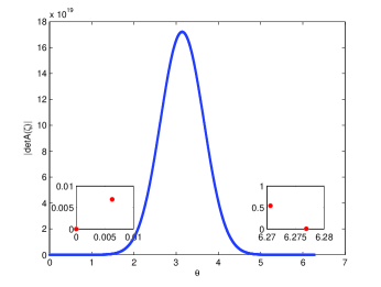
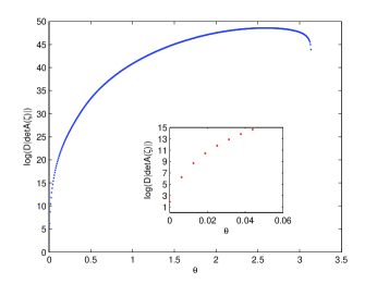
Fig. 2: (left) $\left\lvert\det A(\zeta)\right\rvert$ with $M=1000$; (right) $\log D\left\lvert\det A(\zeta_{i})\right\rvert$. The insets zoom in near the end points.

For mode II, by definition, we have

$$\widetilde{\mathcal{H}}_{\text{CB}}(\partial_{x},\theta)(w_{1},w_{2})^{\mathrm{T}}=\dfrac{2(\kappa_{2}+9\kappa_{4})}{\varepsilon^{2}}\begin{pmatrix}\tfrac{3}{8}(3\partial_{x}^{2}-\theta^{2})&\tfrac{3}{4}\imath\theta\partial_{x}\\[7.22743pt] \tfrac{3}{4}\imath\theta\partial_{x}&\tfrac{3}{8}(\partial_{x}^{2}-3\theta^{2})\end{pmatrix}\begin{pmatrix}w_{1}\\ w_{2}\end{pmatrix}=\begin{pmatrix}0\\ 0\end{pmatrix}.$$

The nonexistence of mode II eigenfunction is equivalent to the fact that the the complementing condition for elliptic PDE [AgmonDouglisNirenberg:1959] is satisfied for the Cauchy-Born problem. For this linearized elasticity problem with boundary condition $\sum_{j=1}^{3}B_{kj}z_{j}(x)=0$ for $k=1,2,3$, the complementing condition is valid by [Thompson:1969] and by explicit calculation

$$\kappa_{2}+9\kappa_{4}=h(1)+9h(\sqrt{3})\geq 60K.$$

Hence mode II eigenfunction does not exist. For mode III, we have $\zeta\to 1$ as $\theta\to 0$, and $z_{1},z_{2}\to 1$. The solution takes the form

$$\lim_{\theta\to 0}z(x_{i},\zeta)=\sum_{k=3}^{6}c_{k}(1)\mathcal{M}_{2}^{\and}(z_{k},1)z_{k}^{i}$$

with $z_{3}=-0.0042,z_{4}=0.0293,z_{5}=0.8945-0.0969\imath$ and $z_{6}=\widebar{z}_{5}$. Substituting the above expression into the last two boundary conditions, we obtain

$$\scriptsize\begin{pmatrix}z_{3}^{-1}\mathcal{M}^{\and}_{22}(z_{3},1)&z_{4}^{-1}\mathcal{M}^{\and}_{22}(z_{4},1)&z_{5}^{-1}\mathcal{M}^{\and}_{22}(z_{5},1)&z_{6}^{-1}\mathcal{M}^{\and}_{22}(z_{6},1)\\ z_{3}^{-1}\mathcal{M}^{\and}_{12}(z_{3},1)&z_{4}^{-1}\mathcal{M}^{\and}_{12}(z_{4},1)&z_{5}^{-1}\mathcal{M}^{\and}_{12}(z_{5},1)&z_{6}^{-1}\mathcal{M}^{\and}_{12}(z_{6},1)\\ z_{3}\mathcal{M}^{\and}_{22}(z_{3},1)&z_{4}\mathcal{M}^{\and}_{22}(z_{4},1)&z_{5}\mathcal{M}^{\and}_{22}(z_{5},1)&z_{6}\mathcal{M}^{\and}_{22}(z_{6},1)\\ z_{3}\mathcal{M}^{\and}_{12}(z_{3},1)&z_{4}\mathcal{M}^{\and}_{12}(z_{4},1)&z_{5}\mathcal{M}^{\and}_{12}(z_{5},1)&z_{6}\mathcal{M}^{\and}_{12}(z_{6},1)\end{pmatrix}\begin{pmatrix}c_{3}(1)\\ c_{4}(1)\\ c_{5}(1)\\ c_{6}(1)\end{pmatrix}=\begin{pmatrix}0\\ 0\\ 0\\ 0\end{pmatrix},$$

which yields $c_{i}(1)=0$ for $i=3,\cdots,6$. This concludes that there does not exist mode III eigenfunction. Therefore, this scheme is stable.

5 Conclusion

We have identified stability conditions, especially stability conditions at the interface, for atomistic-to-continuum hybrid methods with sharp interface. Under these stability conditions, we establish convergence of the hybrid scheme. Though we only consider the flat interface, the analysis can be extended to smooth interface between the atomistic and continuum regions. In that case, we need to check the interface stability condition Assumption C for interface with different angles.

For the example of atomistic-to-continuum coupling method for a triangular lattice considered here, the stability can be checked by hand or with some help of numerical computation. For many other more complicated methods, this might not be easily done. One possible direction is to use numerical methods and symbolic computations to check stability conditions, in analogy to checking GKS conditions for example as in [Thune:1986]. This is an interesting future research direction.

The result in this paper does not apply to transition interface between atomistic and continuum regions that involves corners. The coarsening in the continuum region is also not taken into account. Extension of the results to hybrid schemes with transition interface with corners and with coarsening in the continuum region would be very interesting.