Large Scale Estimation in Cyberphysical Systems using Streaming Data: a Case Study with Smartphone Traces

Abstract

Controlling and analyzing cyberphysical and robotics systems is increasingly becoming a Big Data challenge. Pushing this data to, and processing in the cloud is more efficient than on-board processing. However, current cloud-based solutions are not suitable for the latency requirements of these applications. We present a new concept, Discretized Streams or D-Streams, that enables massively scalable computations on streaming data with latencies as short as a second. We experiment with an implementation of D-Streams on top of the Spark computing framework. We demonstrate the usefulness of this concept with a novel algorithm to estimate vehicular traffic in urban networks. Our online EM algorithm can estimate traffic on a very large city network (the San Francisco Bay Area) by processing tens of thousands of observations per second, with a latency of a few seconds.

Note to Practitioners

This work was driven by the need to estimate vehicular traffic at a large scale, in an online setting, using commodity hardware. Machine Learning algorithms combined with streaming data are not new, but it still requires deep expertise both in Machine Learning and in Computer Systems to achieve large scale computations in a tractable manner. The Streaming Spark project aims at providing an interface that abstracts out all the technical details of the computation platform (cloud, HPC, workstation, etc.).

As shown in this work, Streaming Spark is suitable for implementing and calibrating non-trivial algorithms on a large cluster, and provides an intuitive yet powerful programming interface. The readers are invited to refer to the source code referred in this article for more examples.

This article presents algorithms to sample and compute densities for Gamma random variables restricted to a hyperplane (i.e. distributions of the form $T_{i}|\sum_{j}\alpha_{j}T_{j}=d$ with $T_{j}$ independant Gamma distributions). It is common in this case to use Gaussian random variables because of closed form solutions to solve. If one considers positive valued distributions with heavy tails, our formulas using gamma distributions may be more suitable.

Keyword: Streaming Spark, Arterial traffic estimation.

I Introduction

Cyber-physical systems involve a complex integration of physical and computational processes. Such systems usually integrate two distinct components - (i) a set of sensors that continuously produce streaming data (ii) a set of communication and computation systems that aggregate data and perform data analytics. Large-scale cyber-physical systems can be found everywhere - from intricate control systems used in robotics to complex environment sensing of civil infrastructures. The data produced by such systems can be very large (millions of records/seconds) and the amount of computation necessary to interpret the data can be significant.

Furthermore, over the last decade, the cost of sensing and communication equipment has fallen dramatically to the point that it is less expensive to incorporate a large number of sensors collecting low-value information, rather than judiciously deploying a limited number of sophisticated and more accurate measurement systems. The corresponding fall in costs shifts the burden from carefully designing instrumentation to correctly filtering and interpreting the wealth of information available to the researcher. This paradigm shift leads to two problems: storage and processing. It is not clear which part of the information is relevant so potentially all the information needs to be saved, which may be expensive: in order to find the proverbial needle in the haystack, one needs enough room for the haystack. In addition, small, cheap, unreliable sensors provide information that is more noisy and potentially requires more processing compared to dedicated sensors.

Industries such as genomics and astronomy have learned to cope with extremely large datasets over the last decade. What makes cyberphysical systems truly stand out amongst these applications is the very fast decay of the value of information: in robotics systems for example, the data collected is usually fed into a control system. Past information is often of limited or no value, sometimes as fast as in the span of a few minutes or tens of seconds. This is unlike genomic records which, rather than being processed immediately, need to be stored reliably for a long time. In essence, the incoming information in cyber-physical systems needs to be processed as a stream, and not so much as an ever-growing dataset.

The problem of processing large incoming streams of data has received little attention so far, because most work has focused on adapting existing technologies which are either design scalability or latency but not both. Streaming databases [6] can provide the necessary low latencies but are limited in scalability. On the other hand, scalable batch processing systems like MapReduce or Hadoop [1] are designed for scaling to thousands of machines but perform poorly in terms of latency. Latency is not a concern for many applications, and for these running regular batch jobs with traditional batch systems is appropriate. But this is often insufficient for many cyber-physical systems such as robotics. Working at lower latencies (at the scale of seconds or tens of seconds) presents significant challenges. As a solution to this problem, we use D-Streams [33], a recently proposed programming model where streaming computations are decomposed into a series of batch computations on small time intervals. This model provides two significant benefits.

• Scalability with low latency: Stream processing applications, implemented using D-Streams to scale to large clusters (hundreds of cores) while providing latencies as low as hundreds of milliseconds.

• Simple high-level programming API: The D-Stream abstraction and its associated operations makes it very convenient for a developer to implement complex business logic to process the raw sensor data.

In this article, we investigate the use of Spark Streaming, a system implementing D-Streams, with a large scale estimation problem: inferring the state of traffic on a large road network by using streams of GPS readings. Traffic congestion affects nearly everyone in the world due to the environmental damage and transportation delays it causes. The $2007$ Urban Mobility Report [31] states that traffic congestion causes $4.2$ billion hours of extra travel in the United States every year, which accounts for 2.9 billion extra gallons of fuel and an additional cost of $78 billion. Providing drivers with accurate traffic information reduces the stress associated with congestion and allows drivers to make informed decisions, which generally increases the efficiency of the entire road network [9].

Modeling highway traffic conditions has been well-studied by the transportation community with work dating back to the pioneering work of Lighthill, Whitham and Richards [22]. Recently, researchers demonstrated that estimating highway traffic conditions can be done using only GPS probe vehicle data [32]. Arterial roads, which are major urban city streets that connect population centers within and between cities, provide additional challenges for traffic estimation. Recent studies focusing on estimating real-time arterial traffic conditions have investigated traffic flow reconstruction for single intersections using dedicated traffic sensors. Dedicated traffic sensors are expensive to install, maintain and operate, which limits the number of sensors that governmental agencies can deploy on the road network. The lack of sensor coverage across the arterial network thus motivates the use of GPS probe vehicle data for estimating traffic conditions.

Recent studies focusing on estimating real-time arterial traffic conditions have investigated traffic flow reconstruction for single intersections [27, 10] using dedicated traffic sensors. We consider an estimation engine deployed inside the Mobile Millennium traffic information system [2, 20]. This engine gathers GPS observations from participating vehicles and produces estimates of the travel times on the road network. Mobile Millennium is intended to work at the scale of large metropolitan areas: the road network considered in this work is a real road network (a large portion of the greater Bay Area, comprising 506,685 road links) and the data for this work is collected from thousands of vehicles that generate millions of observations per day. As a consequence of these specifications and requirements, we employ highly scalable traffic algorithms.

The specific problem we address in this use case is how to extract travel time distributions from sparse, noisy GPS measurements collected in real-time from vehicles. A probabilistic model of travel times on the arterial network is presented along with an online Expectation Maximization (EM) algorithm for learning the parameters of this model (Section III). The algorithm is expensive due to the large dimension of the network and the complexity inherent to the evolution of traffic. Furthermore, our EM algorithm has no closed-form expression and requires sampling and non-linear optimization techniques. This is why the use of a distributed system is appropriate. We will present D-Streams in more detail in Section II.

The present work is novel for several reasons. First, it advances research in traffic estimation by presenting a novel travel time estimation algorithm that is highly scalable, uses data commonly available nowadays, and is robust to noise and other random perturbations. This algorithm builds upon a novel statistical distribution: the Gamma-Dirichlet distribution (formally introduced in Appendix A). Second, it shows that it is possible to use complex, multistage filtering algorithms on very large systems with a latencies under a few seconds. Third, it explores the tradeoffs between computational power, timeliness, and accuracy of estimation of the travel times outputs and shows that the estimates gracefully degrade with less data. Fourth, the workflow of this algorithm is representative of a large class of Machine Learning and estimation algorithms. We believe the good system performance results obtained for this particular application (Section IV) hint at potentially significant speedups for other distributed estimation algorithms, and are of interest to researchers using cloud computing for large physical systems, and for the Machine Learning community.

We start by introducing the D-Streams programming model (Section II) and the problem of traffic estimation (Section III). We then give an overview of our estimation algorithm (Section III-B) and we explain how we used Spark Streaming to parallelize the algorithm (Section III-D). We evaluate our implementation in Section IV from the perspective of scalability (Section IV-B) and accuracy (Section IV-C). The derivations related to the properties of the Gamma-Dirichlet distribution are included in the Appendix A.

II Discretized streams: large-scale real-time processing of data streams

Discretized stream (D-Stream) is a recently proposed programming model [33] for processing of streaming data that allows complex machine learning algorithms to be easily expressed and executed on large streams of live data. In this section, we will first discuss the limitations of existing techniques of processing live data. Then we will elaborate on D-Streams highlighting its advantages over existing techniques.

II-A Limitations of current techniques

Current techniques to process large amounts of live streaming data can be broadly classified into the following two categories.

• Using traditional streaming processing systems: Streaming databases like StreamBase [6] and Telegraph [12], and stream processing systems like Storm [28] have been used to meet such processing requirements. While they do achieve low latencies, they either have limited fault-tolerance properties (data lost on machine failure) or limited scalability (cannot be run on large clusters).

• Using traditional batch processing systems: The live data is stored reliably in a replicated file system like HDFS [1] and later processed in large batches (minutes to hours) using traditional batch processing frameworks like Hadoop [1]. By design, these systems can process large volumes of data on large clusters in a fault-tolerant manner, but they can only achieve latencies of minutes at best. Furthermore, the processing model is too low level to conveniently express complex stream computations.

II-B D-Stream - A programming model for stream processing

D-Streams execute deterministic computations similar to those in MapReduce for fault tolerance, but they do so at a much lower latency than previous systems, by keeping state in memory. The input data received from various input sources (e.g., webservices, sensors, etc) during each interval is stored reliably across the cluster to form an input dataset for that interval. Once the time interval completes, this dataset is processed via deterministic parallel operations (like map, filter, reduce, groupBy, etc) to produce new datasets representing program outputs or intermediate states. Finally, these datasets can be saved to external source (databases, etc) or aggregate all the values into some gradient update / expected loss estimate. The advantage of this model is that it provides the developer a convenient high-level programming model to easily express complex stream computations while allowing the underlying system to process the data in small batches thus achieving excellent fault-tolerance properties.

Going into more details, each dataset created in the time intervals is represented as a Resilient Distributed Dataset (RDD) [34] which is an efficient storage abstraction that keeps a distributed collection of data in memory (as opposed to writing it to the disk) to guarantee fast access. A D-Stream is therefore a series of RDDs and lets the user manipulate them collectively through various deterministic parallel operations. We illustrate this abstraction and a few operators with a small program (written for Spark Streaming, an implementation of D-Streams) that computes a running count of page view events by URL.

⬇

val pageViews = readStream("http://...", "1s")

val ones = pageViews.map(evt => (evt.url, 1))

val counts = ones.runningReduce((a, b) => a+b)

This code creates a D-Stream called pageViews by reading an event stream over HTTP, and divides the streams into batches of 1-second intervals. It then transforms the event stream using the map operator to get a D-Stream of (URL, 1) pairs called ones, and performs a running count of these using the runningReduce operator. The arguments to map and runningReduce are Scala syntax for a closure (function literal).

D-Stream operators

D-Streams provide two types of operators to let users build streaming programs:

• Transformation operators, which produce a new D-Stream from one or more parent streams. These can be either stateless (i.e., act independently on each interval) or stateful (share data across intervals).

• Output operators, which let the program write data to external systems (e.g., save processed data to a database).

D-Streams support the same stateless transformations available in typical batch frameworks, including map, reduce, groupBy, and join. In addition, D-Stream also provide stateful operators like windowing and moving average operators that share data across time intervals. The runningReduce operator in the earlier page view program is an example of a stateful operator as it combines page views across time intervals.

Furthermore, since the D-Stream abstraction follow the same processing model as batch systems, the two can naturally be combined. For example, one may not only join two streams of data, but also join a data stream with a batch data - joining a stream of incoming tweets against a pre-computed spam filter or historical data.

Fault-tolerance properties

All the intermediate data computed using D-Stream are by design fault-tolerant, that is, no data is lost if any machine fails. This is achieved by treating each batch of data as an RDD. Each RDD maintains a lineage of operations that was used to create it from the raw input data (stored reliably by the system by automatic replication) [34]. Hence, in the event of failure, if any partition of an RDD is lost, it can be recomputed from raw input data using the lineage. As these operations are deterministic and functional by nature (i.e. side-effect free), the recomputation can be done using fine-grained tasks in parallel on many number. This ensures fast recovery minimizing the effect of the failure on the stream processing system. This novel technique is called parallel-recovery and sets this abstraction apart from existing stream processing systems.

II-C Spark Streaming- An implementation of D-Streams

To implement D-Streams, we use Spark, an existing open-source, batch processing framework, to create Spark Streaming. Spark is a fast, in-memory batch processing framework built on the RDD abstraction, and we naturally extend this framework to implement D-Streams. Both these systems are implemented in Scala [4] (a language based on the Java Virtual Machine), which allows them integrate well with existing Java and Scala libraries for linear algebra, machine learning, etc. Furthermore, the compact syntax of the Scala language hides all the complexities of distribution, replication and data access pattern behind an intuitive programming interface. A relevant portion of the code of the algorithm is provided in Appendix B. This code instantiates a D-Stream with the raw data and derives some other D-Streams that correspond to each step of the algorithm. As can be seen, this code leverages the functional API of Spark and Scala to express stream transformations in a very natural way. Spark Streaming can scale to hundreds of cores while achieving latencies as low as hundreds of milliseconds. We use this system to implement our traffic estimation algorithms, which we shall explain next.

III Scalable traffic estimation from streaming data

We now explain the relevance of D-Streams with a use case of large-scale, low-latency state estimation: vehicular traffic estimation. The goal of the traffic estimation algorithm is to infer the travel times of each link of an arterial road network, given periodic GPS readings from vehicles moving through the network. We will describe in this section our estimation framework. We will discuss the performance gains obtained by using D-Streams in Section IV.

We define the road network as a graph $\mathcal{D}=(\mathcal{V},\mathcal{E})$, where the set $\mathcal{E}$ will be referred to as the “links” of the road network (streets) and $\mathcal{L}$ as the “nodes” (road intersections). For each link $l\in\mathcal{E}$, the algorithm outputs $X_{l}^{t}$, the time it takes at time index $t$ to traverse link $l$. This time is described as a probability distribution parametrized by a vector $\nu_{l}$. Our goal is then to estimate $X^{t}$, the joint distribution of all link travel times across all links in $\mathcal{E}$, for each time index $t$. We assume that the traffic is varying slowly enough that it can be considered a steady state between each evaluation: our algorithm will consider that all the observations between two consecutive time steps have been generated according to the same state. To simplify notations, we will consider a single time interval and drop the reference to time: the joint distribution of travel time is the multidimensional variable $X$.

We will first give an overview of the GPS data that is commercially available today, and an algorithm that converts raw GPS points to map-matched trajectories with high accuracy: the Path Inference Filter (PIF) [19]. We will then present our modeling approach to infer the traffic conditions from these GPS observations. Then we will explain how the Mobile Millennium [20] pipeline implements this algorithm using a computing cloud and Streaming Spark as a computation backend.

III-A Map-matching GPS probe data with the Path Inference Filter

In order to reduce power consumption and transmission costs, probe vehicles do not continuously report their location to the base station. A high temporal resolution gives access to the complete and precise trajectory of the vehicle, but this causes the device to consume more power and communication bandwidth. Also, such data is not available at large scale today, except in a very fragment portion of the the private sector. A low temporal resolution carries some uncertainty as to which trajectory was followed. In the case of a high temporal resolution (typically, a frequency greater than an observation per second), some highly successful methods have been developed for continuous estimation [30, 24, 15]. However, most data collected at large scale today is generated by commercial fleet vehicles. It is primarily used for tracking the vehicles and usually has a low temporal resolution (1 to 2 minutes) [3, 21, 29, 11]. In the span of a minute, a vehicle in a city can cover several blocks (see Figure 1 for an example). Information on the precise path followed by the vehicle is lost. Furthermore, due to GPS localization errors, recovering the location of a vehicle that just sent an observation is a non trivial task: there are usually several streets that could be compatible with any given GPS observation. Simple deterministic algorithms to reconstruct trajectories fail due to misprojection or shortcuts. The Path Inference Filter [19] is a probabilistic framework that recovers trajectories and road positions from low-frequency probe data in real time, and in a computationally efficient manner.

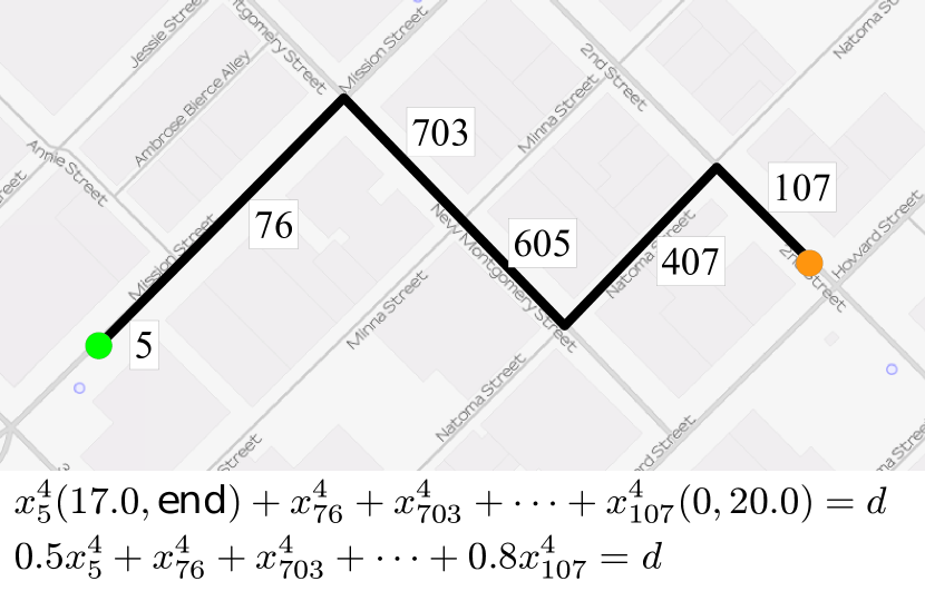
Figure 1: Example of observation. The green mark represents an initial GPS reading, the orange mark represents a subsequent reading. The black line marks the path of the vehicle, as reconstructed by the Path Inference Filter between the two GPS points and the numbers are the indexes of each road link covered by this observation. Given a realization $x^{4}$ of the travel time distribution at time $t=4$, all the information on travel times encoded by this observation is summarized in the equation above.

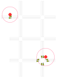
(1) (2)

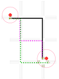
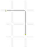
(3) (4)

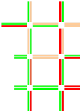
Figure 2: Map-matching algorithm: the raw GPS readings a first projected onto candidate points on the road network (Step 1). Then all feasible paths between each pair of candidate points are computed (Step 2). A dynamic programing algorithm then finds the most likely trajectory, using a Conditional Random Field (Step 3). Trajectory measurements are the input to the Expectation Maximization algorithm. This algorithm outputs distributions of travel times (Step 4).

This algorithm first projects the raw points onto candidate projections on the road network and then builds candidate trajectories to link these candidate projections. An observation model and a driver model are then combined in a Conditional Random Field to find the most probable trajectories, using the Viterbi algorithm. More precisely, the algorithm performs the following steps:

• We map each point of raw (and possibly noisy) GPS data to a collection of nearby candidate projections on the road network (Figure 2-1).

• For each vehicle, we reconstruct the most likely trajectory using a Conditional Random Field  [19] (Figure 2-2).

• Each segment of the trajectory between two GPS points is referred as an trajectory measurement (Figure 2-3). A trajectory measurement consists in a start time, an end time and a route on the road network. This route may span multiple road links, and starts and ends at some offset within some links.

At the output of the PIF, we have transformed sequences of GPS readings into sequences of trajectory readings. These readings are the input for our travel time estimation algorithm.

III-B Fundamental generative model

An example of a trajectory reading is given in Figure 1. Estimating the travel time distributions is made difficult by the fact that we do not observe travel times for individual links. Instead, each reading only specifies the total travel time for an entire list of links traveled. We formally describe our estimation task as a maximum likelihood estimation problem.

We consider one reading, described by an offset on a first road link $o_{\text{start}}$, an offset on a last link $o_{\text{end}}$, a list of $m$ visited links $l_{1}\cdots l_{m}$, a start time, and a travel duration $d$. We simplify the problem by assuming that the partial travel time from the start of a road link to some offset $o$ is proportional to the offset: the travel time between the start of the link $l$ and offset $o$ is a probability distribution $X_{\text{partial}}\left(0,o\right)=\frac{o}{L\left(l\right)}X_{l}$ where $L\left(l\right)$ is the length of link $l$. Using this assumption, we can convert the description of an observation into a vector form: consider the vector $\alpha\in\mathbb{R}^{n}$ where:

$$\alpha\left(l_{1}\right)=1-\frac{o_{\text{start}}}{L\left(l_{1}\right)}$$

$$\alpha\left(l_{m}\right)=\frac{o_{\text{end}}}{L\left(l_{m}\right)}$$

$$\alpha\left(l_{i}\right)=1\text{ for $i\in\left[2...m-1\right]$}$$

and $\alpha\left(l\right)=0$ for all other links $l$. Thanks to the proportionality assumption, the observed travel duration $d$ along the path $p$ is a linear combination of linear travel times:

$$d = \sum_{l\in\mathcal{E}}\alpha\left(l\right)x_{l}$$

$$= \sum_{l\in p}\alpha\left(l\right)x_{l}$$

The vector $\alpha$ is called the path activation vector for this reading. Note that fewer than 10 links are covered in a typical trajectory measurement, so the path activation vectors are extremely sparse. We will use this fact to achieve very good scaling of our algorithm.

For a given time interval, we can completely represent a trajectory reading by an observation $Y=\left(\alpha,d\right)\in\left(\mathbb{R}^{+}\right)^{n}\times\mathbb{R}_{+}^{*}$. Each observation $Y^{\left(r\right)}=\left(\alpha^{\left(r\right)},D^{\left(r\right)}\right)$ describes the $r$th trajectory’s travel time $D^{\left(r\right)}$ and path $\alpha^{\left(r\right)}$ as inferred by earlier stages of the Mobile Millennium pipeline. The travel time $D^{\left(r\right)}$ is the time interval between consecutive GPS observations and is roughly one minute for our source of data.

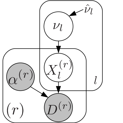
Figure 3: Directed (Bayesian) graph of the travel time model. Grey nodes are observed variables, white nodes are hidden variables. The arrows represent conditional dependencies between the variables. Boxes encode plates, i.e. a factorization of repeating variables. (Right) an expansion of a few elements of the plates.

To make the inference problem tractable, we model the link travel times for each link $l$ as a Gamma distribution with parameter vector $\nu_{l}=\left(k_{l},\theta_{l}\right)$, and we assume these distributions are pairwise independent. The independence assumption is standard in the transportation literature [17, 18] and it also leads to a highly scalable estimation algorithm. We will discuss the validity of this assumption in Section IV-C.

The dependencies between the observations and the parameter vector $\nu$ can be represented as a Bayesian graphical model, which encodes all the dependencies between the variables in a very compact form (Figure III-B). We now formalize the problem of estimating the set of parameters $\nu=\left(\nu_{l}\right)_{l}\in\mathbb{R}^{n\times 2}$ for a set of observations $\left(Y^{\left(r\right)}\right)_{r=1\cdots R}$ as a learning problem. We consider that the the current estimate of the traffic is completely described by independent Gamma distributions of the travel times over each road link. These travel times are (indirectly) observed through a set of observations $Y^{\left(r\right)}=\left(\alpha^{\left(r\right)},d^{\left(r\right)}\right)$. The set of parameters that maximizes the likelihood of these observations is solution to the maximum likelihood problem:

$$\max_{\nu}\,\,ll\left(Y;\nu\right) = \sum_{r}\log\pi\left(D^{\left(r\right)}\bigg{|}\alpha^{\left(r\right)};\nu\right)$$ (1)

with $\pi\left(D^{\left(r\right)}\bigg{|}\alpha^{\left(r\right)};\nu\right)$ the probability of observing the duration $d=\sum_{l}\left(\alpha\left(l\right)\right)x_{l}$ when $x_{l}$ is generated according to the distribution $\pi\left(\cdot;\nu_{l}\right)$. This likelihood can be decomposed using the relations of independence between variables:

$$\pi\left(D^{\left(r\right)}\bigg{|}\alpha^{\left(r\right)};\nu\right)=\int_{X}\pi\left(D^{\left(r\right)}\bigg{|}X,\alpha^{\left(i\right)}\right)\pi\left(X;\nu\right)\text{d}X$$

$$=\int_{X}\pi\left(D^{\left(r\right)}\bigg{|}X,\alpha^{\left(i\right)}\right)\left(\prod_{l\,:\,\alpha^{\left(r\right)}\left(l\right)>0}\pi\left(X_{l};\nu_{l}\right)\text{d}X_{l}\right)$$

$$=\int_{X}\pi\left(D^{\left(r\right)}\bigg{|}X,\alpha^{\left(i\right)}\right)\left(\prod_{l\,:\,\alpha^{\left(r\right)}\left(l\right)>0}\pi\left(X_{l};\nu_{l}\right)\text{d}X_{l}\right)$$

Estimating the travel time distributions is made difficult by the fact that we do not observe travel times $X$ for individual links. Instead, each observation only specifies the total travel time $D$ for an entire list $\alpha$ of links traveled. To get around this problem, we use the Expectation Maximization (EM) algorithm [13, 26]. The EM algorithm operates in two phases: In the E-step it considers each travel time measurement and computes a distribution over allocations of travel time to each of the links. In the M-step it computes the link parameters that maximizes the likelihood of the travel times for the allocations made in the E-step. By iterating this process the EM algorithm converges to a set of link parameters that are a local maximum of the likelihood of the data. In our setting, we run the EM algorithm in an online fashion: for each time step, we use the previous time step as a value, perform a few (iterations and we monitor the convergence through the expected complete log-likelihood. This form of online EM gives good results for our application (Section IV).

While this model is relatively simple, the use of Gamma distributions substantially complicates the E step, because sums of independent Gamma distributions have no simple form. A correct computation of the expected complete log-likelihood requires the normalization constant of each distribution $X^{\left(r\right)}|\left(\alpha^{\left(r\right)}\right)^{T}X^{\left(r\right)}=D^{\left(r\right)}$. Computing this normalization factor for each observation is fairly expensive (it uses an infinite series expansion) and is critical for good accuracy in practice. These practical considerations are described in the next section, and the computational burden justifies the need for cloud computing.

III-C Learning with Gamma distributions

In the previous section, an observation was defined by a duration $d>0$ and a (sparse) vector $\alpha\in\left(\mathbb{R}_{+}^{*}\right)^{n}$, with the constraint:

$$d=\alpha^{T}x$$ (2)

where $x$ is a vector of unobserved samples from independent Gamma distributions. The Expectation-Maximization algorithm relies on two operations: computing the conditional distribution $\pi\left(x|d,\alpha;\nu\right)$ of the vector $x$ when $\alpha$ and $d$ are known and the parameter vector $\nu$ is fixed, and sampling this distribution, i.e. computing $x$ so that $x_{l}\sim\Gamma\left(k_{l},\theta_{l}\right)$ under the constraint 2. In the case of Gamma distributions, some formulas exist for these operations. For the sake of clarity, we only present the main results here, without proof or background. The reader is invited to refer to Appendix A for a longer exposure.

Sampling from conditional gamma distributions. Consider a set of $n$ independent Gamma distributions $T_{i}\sim\Gamma\left({k}_{i},\theta_{i}\right)$ with $k\in\left(\mathbb{R}_{+}^{*}\right)^{n}$ and $\theta\in\left(\mathbb{R}_{+}^{*}\right)^{n}$, a $n$-dimensional vector of positive numbers $\alpha\in\left(\mathbb{R}_{+}^{*}\right)^{n}$ and $d>0$. Call $T$ the joint distribution of all $T_{i}$s. The purpose of this paragraph is to present some practical formulas to sample and compute the density function of the conditional distribution:

$$Z\sim T\bigg{|}\sum_{i}\alpha_{i}T_{i}=d$$

We define this distribution over the $n$-dimensional simplex $\mathcal{S}_{\alpha,d}$:

$$\mathcal{S}_{\alpha,d}=\left\{x\in\left(\mathbb{R}^{+}\right)\bigg{|}\alpha^{T}x=d\right\}$$

Using an appropriate probability measure over the set $\mathcal{S}_{\alpha,d}$, the probability density function of $Z$ is:

$$f\left(z\right)=\frac{1}{n\kappa\left(k,\hat{\theta}\right)}d^{n-1}\frac{\sqrt{\sum_{i}\alpha_{i}^{2}}}{\prod_{i=1}^{n}\alpha_{i}}\prod_{i}f_{\Gamma}\left(\frac{\alpha_{i}z_{i}}{d};k_{i},\hat{\theta}_{i}\right)$$ (3)

with:

$$\hat{\theta}_{i}=d^{-1}\alpha_{i}\theta_{i}$$

and $f_{\Gamma}$ the density function of the Gamma distribution: $f_{\Gamma}\left(x;\tilde{k},\tilde{\theta}\right)=\Gamma\left(\tilde{k}\right)^{-1}\theta^{-\tilde{k}}x^{\tilde{k}-1}e^{-\tilde{\theta}^{-1}x}$. The normalization factor $\kappa\left({k},\hat{\theta}\right)$ can be described by an infinite series, and is a straightforward adaptation of a result from Moshopoulos [25]. The proof is provided in Appendix A and uses a new distribution, called the Gamma-Dirichlet distribution, that generalizes the Dirichlet distribution.

Given $\alpha\in\left(\mathbb{R}_{+}^{*}\right)^{n}$ and $d>0$.

Generate $n$ independent samples $a_{i}\sim\Gamma\left({k}_{i},d^{-1}\alpha_{i}\theta_{i}\right)$

$z_{i}=d\alpha_{i}^{-1}\frac{a_{i}}{\sum_{k}a_{k}}$

Then $z\sim Z|\alpha^{T}Z=d$

Algorithm 1 Sampler for Gamma distributions conditioned on a hyperplane

Sampling algorithm. There happens to exist a straightforward procedure to sample values from the conditional Gamma distribution $Z$, presented in Algorithm 1. A proof that this algorithm gives the intended result is also given in Appendix A.

III-D Overview of the MM arterial pipeline

The Mobile Millennium system incorporates a complete pipeline for receiving probe data, filtering it, distributing it to estimation engines and displaying it, all in in real-time. This software stack, written in Java and Scala, evaluates probabilistic distribution of travel times over the road links, and uses as input the sparse, noisy GPS measurements from probe vehicles.

The most computation-intensive parts of this pipeline have all been ported to a cloud environment. We briefly describe the operations of the pipeline, pictured in Figure 4.

The observations are grouped into time intervals and sent to a traffic estimation engine, which runs the learning algorithm described in the next section and returns distributions of travel times for each link (Figure 2).

The travel time distributions are then stored and broadcast to clients and to a web interface. Examples of means of travel times are shown in Figure 6.

It is important to point out that Mobile Millennium is intended to work at the scale of large metropolitan areas. The road network considered in this work is a real road network (a large portion of San Francisco downtown and of the greater Bay Area, comprising 506,685 road links) and the data is collected from the field (as opposed to simulated). A consequence of this setting is the scalability requirement for the traffic algorithms we employ. Thus, from the outset, our research has focused on designing algorithms that could work for large urban areas with hundreds of thousands of links and millions of observations.

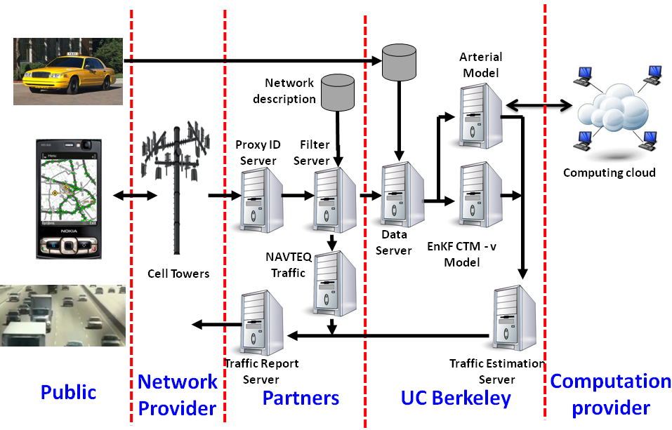
Figure 4: Schematic architecture of the Mobile Millennium system.

Our algorithm needs to run expensive computations in an iterative fashion on incoming streaming data. As such, it is a perfect candidate for D-Streams. We now describe how we parallelized the EM algorithm using Spark’s implementation of D-Streams.

Figure 5 shows the data flow in the algorithm in more detail. In the E-step, we generate per-link travel time samples from whole observations; specifically, for each observation $Y^{\left(r\right)}=\left(\alpha^{\left(r\right)},d^{\left(r\right)}\right)$, we produce a set of $U$ weighted samples $\mathbf{X}^{\left(r\right)}=\left\{\left(x^{\left(r,u\right)},w^{\left(r,u\right)}\right)\right\}_{u=1\cdots U}$, each sample $x^{\left(r,u\right)}$ produced by randomly dividing travel time $d^{\left(r\right)}$ among its constituent links (producing a travel time $x_{l_{i}}^{\left(r,u\right)}$ for each edge $l_{i}\in\alpha^{\left(r\right)}$). We assign a weight $w^{\left(r,u\right)}$ as the likelihood of travel time $x^{\left(r,u\right)}$ according to the current distribution parameters $\nu$. In the shuffle step, we regroup the samples $\mathbf{X}^{\left(r\right)}$ by link, so that each link $l$ now has samples $\tilde{\mathbf{X}}_{l}=\left\{\left(s_{l}^{\left(r,u\right)},w_{l}^{\left(r,u\right)}\right)\right\}_{r,u}$ from all the observations $r$ that go over it. In the M-step, we recompute the parameters $\nu_{l}$ to fit link $l$’s travel time distribution to the samples $\tilde{\mathbf{X}}_{l}$.

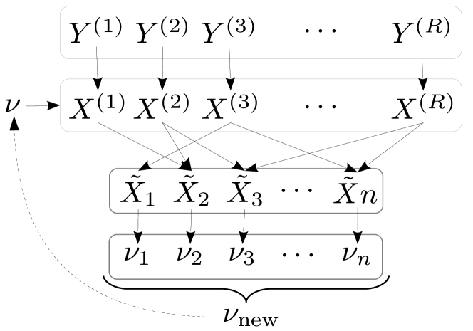
Figure 5: System workflow of the EM algorithm. In the E-step, we generate per-link travel time samples from whole observations; specifically, for each observation $Y^{\left(r\right)}=\left(\alpha^{\left(r\right)},d^{\left(r\right)}\right)$, we produce a set of $U$ weighted samples $\mathbf{X}^{\left(r\right)}=\left\{\left(x^{\left(r,u\right)},w^{\left(r,u\right)}\right)\right\}_{u=1\cdots U}$, each sample $x^{\left(r,u\right)}$ produced by randomly dividing travel time $d^{\left(r\right)}$ among its constituent links (producing a travel time $x_{l_{i}}^{\left(r,u\right)}$ for each edge $l_{i}\in\alpha^{\left(r\right)}$). We assign a weight $w^{\left(r,u\right)}$ as the likelihood of travel time $x^{\left(r,u\right)}$ according to the current distribution parameters $\nu$. In the shuffle step, we regroup the samples $\mathbf{X}^{\left(r\right)}$ by link, so that each link $l$ now has samples $\tilde{\mathbf{X}}_{l}=\left\{\left(s_{l}^{\left(r,u\right)},w_{l}^{\left(r,u\right)}\right)\right\}_{r,u}$ from all the observations $r$ that go over it. In the M-step, we recompute the parameters $\nu_{l}$ to fit link $l$’s travel time distribution to the samples $\tilde{\mathbf{X}}_{l}$.

We note that our EM algorithm is representative of a large class of iterative machine learning algorithms, including clustering, classification, and regression methods, for which popular cloud programming frameworks like Hadoop and Dryad are often inefficient [16, 23]. Our lessons with Streaming Spark are likely applicable to these applications too.

IV A case study: taxis in the San Francisco Bay Area

Having now described an algorithm for computing travel time distributions in real time on a road network, we describe our validation experiments. These experiments explore two settings:

• The raw performance of the machine learning algorithm, given a limited amount of data and a computational budget,

• The performance of the Streaming Spark framework in distributing computations across a cluster, and the computational performance improvement gained by additional hardware.

The performance of the algorithm is computed by asking the model to give travel time distributions on unseen trajectories, slightly in the future. The observed travel time of the trajectory is then compared with the distribution provided by the model. We measured the L1 and L2 losses between the observed travel time and the distribution mean, and the likelihood of the observed travel time with respect to the predicted travel time distribution. This is done with different amount of data and different time horizons.

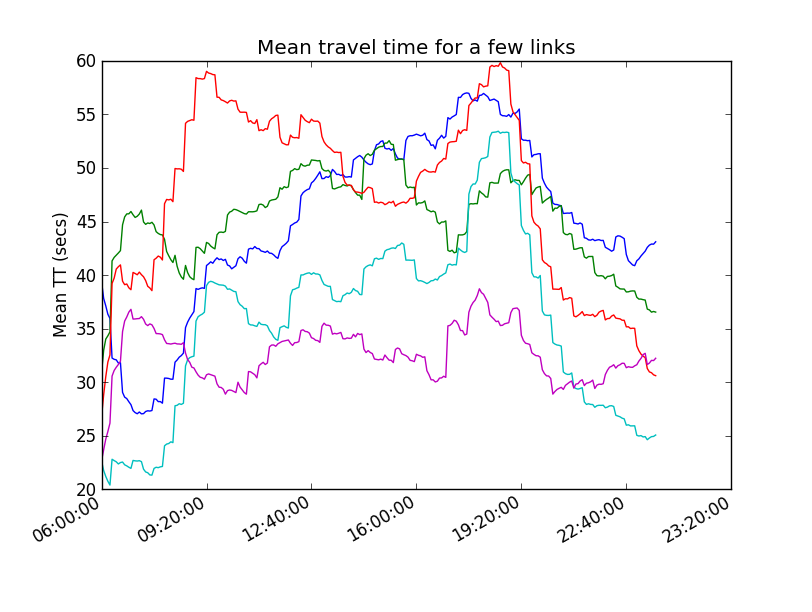
Figure 6: An example output of traffic estimates from our algorithm: mean travel times on different road links in the business district of San Francisco during a complete day.

The computational efficiency of the algorithm is validated in two steps. First, we demonstrate that our algorithm scales well: given twice as many computation nodes, it perform the same task about twice as fast. We also see that this algorithm is bounded by computations. Then, we demonstrate that it can sustain massive data flow rates under strict scheduling constraints: we fix a completion time of a few seconds for each time step, and we find the maximum flow rate under a given computational budget.

IV-A Taxis in San Francisco

Our implementation was run on a road network that corresponds to the greater San Francisco Bay Area (506,685 road links), using some taxi data provided by the Cabspotting project [11]. This dataset contains GPS samples of a few thousand taxicabs emitted every minute, for more than a year. All in all, it represents hundred of millions of GPS points. We ran our algorithm on a typical day (August 12th 2010, a Tuesday) with different settings. An example of input data is given in Figure 7. A typical output of travel times provided by the algorithm is given in Figure 6.

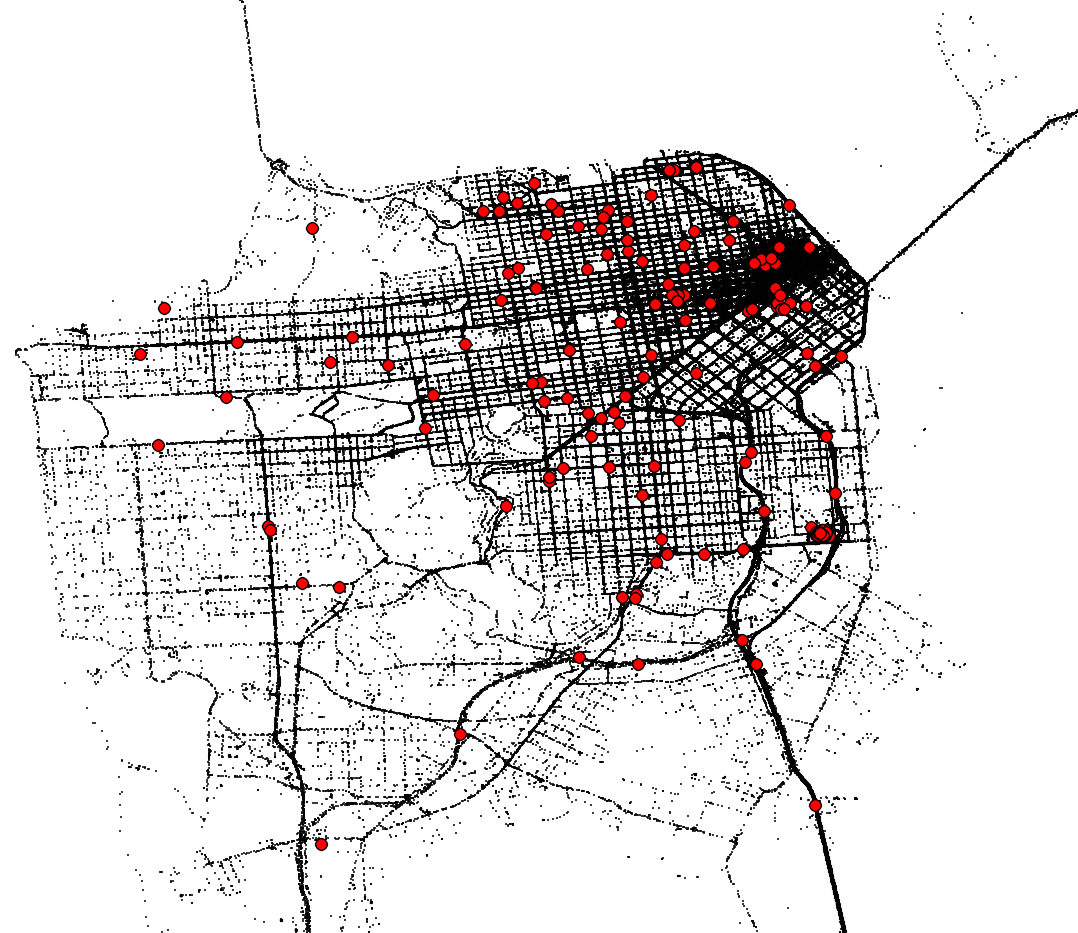
Figure 7: An example of dataset available to Mobile Millennium and processed by the path inference filter: taxicabs in San Francisco from the Cabspotting program. Large circles in red show the position of the taxis at a given time and small dots (in black) show past positions (during the last five hours) of the fleet. The position of each vehicle is observed every minute.

IV-B Good scalability results using a large cluster

In this section, we evaluate how much the cloud implementation helped with scaling the Mobile Millennium EM traffic estimation algorithm. Distributing the computation across machines provides a twofold advantage: each machine can perform computations in parallel, and the overall amount of memory available is much greater.

Scaling. First, we evaluated how the runtime performance of the EM job could improve with an increasing number of nodes/cores. The job was to learn some historical traffic estimate for San Francisco downtown for a half-hour time-slice, using a large portion of the data split in one-hour intervals. This data included 259,215 observed trajectories, and the network consisted of 15,398 road links. We ran the experiment on two cloud platforms: the first was using Amazon EC2 m1.large instances with 2 cores per node, and the second was a cloud managed by the National Energy Research Scientific Computing Center (NERSC) with 4 cores per node. Figure 8 (bottom) shows near-linear scaling on EC2 until 80–160 cores. Figure 8 (top) shows near-linear scaling for all the NERSC experiments. The limiting factor for EC2 seems to have been network performance. In particular, some tasks were lost due to repeated connection timeouts.

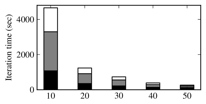
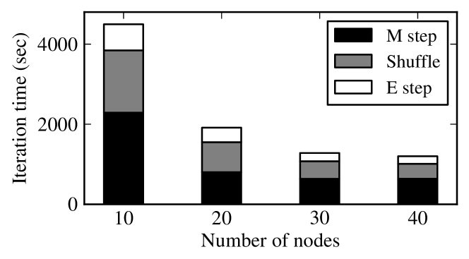
Figure 8: Experiments with Spark to build historical estimates of traffic, on NERSC (top) and Amazon EC2 (bottom).

Scaling on Streaming Spark. After having found the bottlenecks in the Spark program, we wrote another version in Streaming Spark. The two programs are strikingly similar (see program listing in Appendix B). We then benchmarked the application. We ported this application to Spark Streaming using an online version of the EM algorithm that merges in new data every five seconds. The implementation was about 200 lines of Spark Streaming code, and wrapped the existing map and reduce functions in the offline program. In addition, we found that only using the real-time data could cause overfitting, because the data received in five seconds is so sparse. We took advantage of D-Streams to also combine this data with historical data from the same time during the past 10 days to resolve this problem. Figure 9 shows the performance of the algorithm on up to 80 quad-core EC2 nodes. The algorithm scales almost perfectly, largely because it is so CPU-bound, and provides answers an order of magnitude faster than the previous implementation.

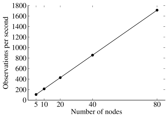
Figure 9: Experiments with Streaming Spark: rate of observation processing for different cluster sizes.

IV-C Our algorithm can be adjusted for trade-offs between amount of data, computational resources and quality of the output

We now study the accuracy of our algorithm in estimating the traffic. Even if we receive a large number of observations per day, this number is not sufficient to cover properly in real time all the road network: indeed, some sections of the road network are much less traveled than the busy downtown areas. We use several strategies to mitigate this spatial discrepancy:

• We use a prior on the Gamma distribution, itself a Gamma distribution since the Gamma is in the exponential family and conjugate with itself. The parameters of this prior are to 70% of the speed limit in mean and 1 minute or 50% of the travel time in standard deviation, whichever is greater.

• We incorporate some data from the same day before the current time step, weighted by an exponential decay scheme: the traffic in the arterial network is assumed to change slowly enough.

• We also incorporate some data from previous days, corresponding to the same day of the week (Monday, Tuesday, etc.). Traffic is expected to follow a weekly pattern during the same month.

To summarize, a large number of observations are lumped together and weighted according to the formula:

$$w=e^{-\Delta t_{\text{day}}^{-1}\left(t_{\text{obs}}-t_{\text{current}}\right)}e^{-\Delta t_{\text{week}}^{-1}\left(week_{\text{obs}}-week_{\text{current}}\right)}$$

The half-time decaying factors $\Delta t_{\text{day}}$ and $\Delta t_{\text{week}}$ are set so that the corresponding weight is 0.2 at the end of the window.

Since the EM learning algorithm is not linear in the observations, we cannot reduce each observation to some sufficient statistics. As the algorithm moves forward in time, each observation will appear at different time steps with a different weight and needs to be reprocessed. This is a significant limitation from this approach, but it makes for a good testing ground of Streaming Spark.

Our EM algorithm can be adjusted in several ways:

• The number of weeks of data to look back (between 1 and 10)

• The time window to consider before the current observation (between 20 minutes and 2 hours)

• The number of samples generated during the E-steps (10-100)

• The number of EM iterations (1-5)

• The duration of each time step (5 seconds-15 minutes)

The observations we process all have a duration of one minute, but travel times experienced by users are usually much longer (10 minutes to a few hours). As such, a good metric for assessing the quality of a model should not be on predicting travel times for one-minute observations, but on longer distances. Hour-long travels are very likely to go be spent mostly on highways, which is not the scope of this study, and taxicabs usually make small trips (10 to 30 minutes). This is why we focus our attention to travel times between one minute (the observations) and 30 minutes (typical durations for taxi rides). As far as we know, this study of different durations is seldom done in the study of traffic, which limits any attempt to compare the performance between different algorithms.

The longer trajectories are obtained from the Path Inference Filter. They are then cuts into different pieces of the same length (1 minute, 5 minutes, 10 minutes, 20 minutes). Each piece of trajectory is considered as an independent piece of trajectory for the purpose of travel time prediction.

We ran the algorithm with 4 different settings:

• SlidingBig: the most expensive setting (10 weeks of data, 2 hours of data, 100 EM samples, 5 EM iterations, 15 time steps), used as the baseline for comparison. Travel time estimates are produced every 20 minutes,

• SlidingBig1: uses less data (40 minutes of data),

• SlidingBig2: uses less data (10 days),

• SlidingBig3: uses the same amount of data, but performs only a single EM iteration every 4 minutes instead of 5 EM iterations every 20 minutes,

• SlidingBig4: uses the same amount of data, but generates only 10 EM samples for each observation

For all these experiments, the prior was fixed.

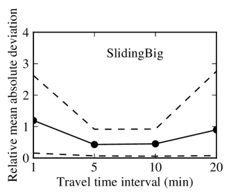
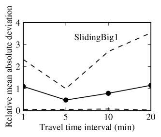
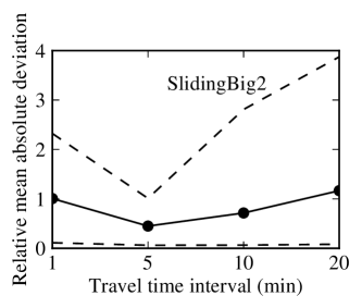
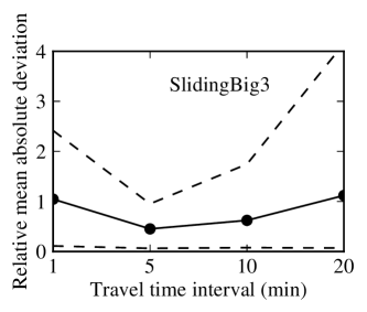
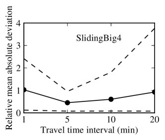
Figure 10: L1 residuals for different settings and for different travel times. The dashed lines indicate the 95% confidence interval. On the $x$ axis, the travel time of the the observations considered for this metric.

We now compare the results obtained with the different experiments. We first turn our attention to the L1 loss in Figure 10. As expected, the best performance is obtained for experiment SlidingBig, which uses the most data. Interestingly enough, the best performance is obtained for travels of medium length (4-11 minutes), and not for short trajectories. This can be explained by the conversion step that transforms trajectory readings on partial links into weighted observations on complete links. The relation between link travel time and location on a link is more complex than a linear weighting. Nevertheless, the model gives relatively good performance by this simple transform. When a vehicle is stopped at a red light, it does not travel along the link but still has a non-zero travel time. In this case, the weight of an observation is taken to be half of the total travel time of the link. In particular, the relative error increases as the duration (and the length) of travels increases. Performance is not too different between experiments, which suggests some even smaller amount of data could be considered.

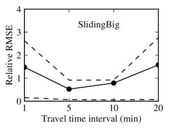
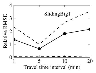
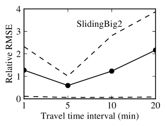
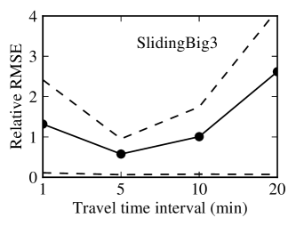
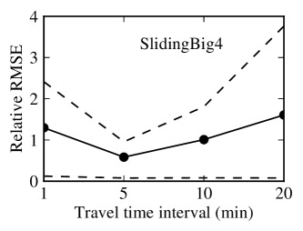
Figure 11: L2 residuals for different settings and for different travel times. The dashed lines indicate the 95% confidence interval.

The results for the L2 loss, presented in Figure 11, provide some similar, if more acute, results. The RMSE is lowest for small to medium travels (in the range of 3-10 minutes).

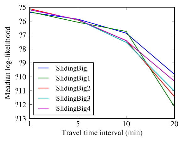
Figure 12: Log-likelihood of unobserved trajectories, for different trajectory lengths and different settings.

A probabilistic metric (the log-likelihood) gives a different insight, as shown in Figure 12. The model best explains the data for very short travel times (similar to what is was trained on) but its precision falls down as the length of trajectories increases. All in all, this results should not be unexpected: this model with independent links cannot take into account the correlations that occur due to light synchronizations or drivers’ behavior. As such, the probability density of a longer travel rapidly dilutes as the number of links increases As we saw with our study of L1 and L2 errors, the mean travel time becomes the only significant value of interest for longer travel times. In the light of this result, there seems to be little to gain by modeling travel time with physically realistic, link-based, independent distributions, as the independence assumption will strongly weigh on the quality of the travel time for longer travels. Instead, we recommend focusing effort on simpler models of travel times that take into account the correlations between links.

Conclusion

As datasets grow in size, some new strategies are required to perform meaningful computations in a short amount of time. We explored using a new technique, Discretized Streams or D-Streams, that offers some significant advantages for implementing large-scale state estimation in near-real-time. D-Streams were implemented in the Spark computing framework. This approach was validated with a real-life, large-scale estimation problem: vehicular traffic estimation. Our traffic algorithm is an Expectation-Maximization algorithm that computes travel time distributions of traffic by incremental online updates. This algorithm seems to compare favorably with the state of the art and shows some attractive features from an implementation perspective. When distributed on a cluster, this algorithm scales to very large road networks (half a million road links, tens of thousands of observations per second) and can update traffic state in a few seconds.

In order to foster research in systems and in traffic, the authors have released the code of Spark Streaming [5], the code of the EM traffic algorithm [7], and the dataset used for these experiments [7].

Appendix A: The Gamma-Dirichlet distribution

We provide proofs and more detailed exposure to the claims made in Section III-B. We formally introduce a straightforward generalization of the Dirichlet distribution, which we call the Gamma-Dirichlet distribution. We detail the derivation of the p.d.f. and the sampling procedures of the conditional distribution $Z|\alpha^{T}Z=t$.

The Gamma-Dirichlet distribution. The regular simplex $\mathcal{S}^{n}\subset\mathbb{R}^{n}$ is the convex hull of the elementary vertices $\left(\mathbf{e}_{i}\right)_{i\in\left[1,n\right]}$. Given a vector ${k}\in\left(\mathbb{R}^{+}\right)^{n}$ and a vector $\theta\in\left(\mathbb{R}^{+}\right)^{n}$, we define the Gamma-Dirichlet distribution:

$$X\sim\Gamma D\left({k},\theta\right)$$

with values over the regular simplex $\mathcal{S}^{n}$ as the normalized sum of $n$ elements drawn from independent Gamma distributions:

$$X_{i}=\frac{Y_{i}}{\sum_{j}Y_{j}}$$

with

$$Y_{i}\sim\Gamma\left({k}_{i},\theta_{i}\right)$$ (4)

and $Y_{i}$ all pairwise independent. The Gamma-Dirichlet distribution is a simple generalization of the Dirichlet distribution: if $\theta=a\mathbf{1}$ for some $a>0$, this is the Dirichlet distribution of the $n$th order. The definition gives a straightforward procedure to sample some values from $X$. We now present some new results: we give a formula for the density function that is amenable for computations and we describe some heuristics that speed up computations by some significant margin with no significant loss of precision in practice. Finally, we study the relation between the Gamma-Dirichlet distribution and the conditional distribution $Z|\alpha^{T}Z=d$, in which a vector of independent Gamma distributions is jointly constrained on a hyperplane. Specifically, we show this distribution over $Z$ is equivalent to the Gamma-Dirichlet distribution.

Density. Note first that one needs to be careful in defining the underlying $\sigma$-algebra of our probability space, as the values of $X$ are located in an embedding of $\mathbb{R}^{n}$ of measure $0$ (a hyperplane). Consider the $n$-dimensional hyperplane $\mathcal{H}^{n}=\left\{x|x^{T}\mathbf{1}=1\right\}$. This hyperplane includes the simplex $\mathcal{S}^{n}$. The Lebesgue measure of this set in $\mathbb{R}^{n}$ is zero. However, we can consider the Lebesgue measure $\tilde{\mu}$ defined over $\mathbb{R}^{n-1}$ and the transform: $\phi:\mathbb{R}^{n-1}\rightarrow\mathcal{H}^{n}$ defined by $\phi\left(u\right)=\left(u^{T}\mathbf{1}-\sum_{j}u_{j}\right)^{T}$. This transform is a mapping, so it lets us define a new measure $\hat{\mu}$ for the space $\mathcal{H}^{n}$ based on $\tilde{\mu}$. Under this measure, the measure of the simplex $\mathcal{S}^{n}$ is positive. Call $\mu$ the measure defined over $\mathcal{S}^{n}$ by $\mu\left(\cdot\right)=\hat{\mu}\left(\mathcal{S}^{n}\right)^{-1}\hat{\mu}\left(\cdot\right)$. With respect to this measure, the Gamma-Dirichlet distribution has density function:

$$f\left(x\right)=\kappa\left({k},\theta\right)^{-1}\prod_{i=1}^{n}f_{\Gamma}\left(x_{i};{k}_{i},\theta_{i}\right)$$

with $f_{\Gamma}\left(x;k,\theta\right)$ the p.d.f. of the gamma distribution: $f_{\Gamma}\left(x;k,\theta\right)=\Gamma\left(k\right)^{-1}\theta^{-k}x^{k-1}e^{-\theta^{-1}x}$. The normalization factor $\kappa\left({k},\theta\right)$ is defined by an infinite series, based on a result of Moschopoulos [25]:

$$\kappa\left(k,\theta\right)=\left(\prod_{i=1}^{n}{k}_{i}^{-\theta_{i}}\right)e^{-1/\tilde{k}}\sum_{l=0}^{\infty}\frac{\delta_{l}}{\tilde{k}^{l}\Gamma\left(\tilde{\theta}+l\right)}$$

with

$$\tilde{k}=\sum_{i}{k}_{i}$$

and $\left(\delta_{j}\right)_{j}$ a series defined by the recursive formula:

$$\begin{cases}\delta_{0}=&1\\ \delta_{l}=&\frac{1}{l}\sum_{m=0}^{l}\delta_{l}\left(\sum_{i=1}^{n}k_{i}\rho_{i}^{l-m}\right)\end{cases}$$

Proof:

This result can be obtained by first proving the equivalence of the Gamma-Dirichlet distribution with the conditional distribution $Z|\sum_{j}Z_{j}=1$, which is done below and does not need the scaling constant $\kappa$. Now, consider the distribution of the normalization factor $Y=\sum_{j}Y_{j}$. This variable is a sum of independent Gamma variables, with p.d.f $f_{Y}$. Then $\kappa\left({k},\theta\right)=f_{Y}\left(1.0\right)$. An expression for this coefficient in terms of a converging series of Gamma coefficients is given in [25, 8]. ∎

The computation of $\delta_{i}$ is quadratic in time, which can be too slow if tens of thousands of coefficients are required before convergence, as it may happen in our application. We present below some heuristics to speed up the computations of this sequence.

Equivalence with conditional Gammas. Consider the conditional distribution $Z_{i}=Y_{i}|\sum_{j}Y_{j}=1$ with $Y_{i}$ defined in Equation 4. The density function of this distribution is $0$ over $\mathbb{R}^{n}$ nearly everywhere, however it has non-zero measure over the regular simplex $\mathcal{S}^{n}$. Given a measure $\mu$ defined over $\mathcal{S}^{n}$, the two distributions are the same:

$$\forall x\in\mathcal{S}^{n},\,\,f_{\Gamma D}\left(x\right)=f\left(x\right)$$

Proof:

This proof is adapted from a similar proof [14] for the Dirichlet distribution. Using the same notations as above, define $Y=\sum_{j}Y_{j}$ and $X_{i}=Y_{i}/Y$ for $i\leq n-1$. The joint density for the $Y$’s is:

$$f\left(y\right)\propto\prod_{i}y_{i}^{{k}_{i}-1}e^{-\sum\theta_{i}^{-1}y_{i}}$$

Define the transform $\tilde{\varphi}:\,\mathbb{R}^{n}\rightarrow\mathbb{R}^{n}$ by: $\tilde{y}=\sum_{i}\theta_{i}^{-1}y_{i}$ and $\tilde{x}_{i}=\tilde{y}^{-1}\theta_{i}^{-1}y_{i}$ for $i\leq n-1$. This mapping is invertible and its Jacobian at $\tilde{y}$ is $\left(\prod_{i}\theta_{i}^{-1}\right)\tilde{y}$. Thus the joint density of $\left(\tilde{y},\tilde{x}\right)$ is:

$$g\left(\tilde{y},\tilde{x}\right)\propto\left(1-\sum_{i=1}^{n-1}\tilde{x}_{i}\right)^{{k}_{n}-1}\prod_{i=1}^{n-1}\tilde{x}_{i}^{{k}_{i}-1}\tilde{y}^{\sum_{i}{k}_{i}-1}e^{-\tilde{y}}$$

This shows that the variables $\tilde{y}$ and $\tilde{x}$ are independent, and that the distribution of $\tilde{x}$ is a Dirichlet distribution.

Define the transform $\varphi:\,y=\sum_{i}y_{i}$ and $x_{i}=y^{-1}y_{i}$ for $k\leq n-1$. This mapping is also invertible, with Jacobin $y^{k}$. The joint density of $\left(y,x\right)$ is:

$$g\left(y,x\right)\propto\left(1-\sum_{i=1}^{n-1}x_{i}\right)^{{k}_{n}-1}\prod_{i=1}^{n-1}x_{i}^{{k}_{i}-1}y^{\sum_{i}{k}_{i}-1}e^{-y\sum_{i}\theta^{-1}x_{i}}$$

By identification, we get: $g\left(x|y=1\right)=g\left(\Delta^{-1}\tilde{x}\right)$ with $\Delta$ the diagonal matrix defined by $\Delta_{ii}=\theta_{i}$. Since $\tilde{\varphi}^{-1}\left(\left(\Delta^{-1}\tilde{x},1\right)^{T}\right)=\tilde{x}$, the result ensues. ∎

Sampling from conditional gamma distributions. Consider a set of $n$ independent Gamma distributions $T_{i}\sim\Gamma\left(k_{i},\theta_{i}\right)$, a $n$-dimensional vector of positive numbers $\alpha\in\left(\mathbb{R}_{+}^{*}\right)^{n}$ and $t>0$. The purpose of this section is to present some practical formulas to sample and compute the density function of the conditional distribution:

$$Z=T\bigg{|}\sum_{i}\alpha_{i}T_{i}=t$$

We define this distribution over the $n$-dimensional simplex

$$\mathcal{S}_{\alpha,t}=\left\{x\in\left(\mathbb{R}^{+}\right)\bigg{|}\alpha^{T}x=t\right\}$$

As before, we define a new measure over the hyperplane defined by $\alpha^{T}x=t$, and use it as our base measure $\text{d}z$ for $Z$. We call $f$ the probability density function of variable $Z$ with respect to this measure. With respect to this measure, the probability density function of $Z$ is that of a Gamma-Dirichlet distribution:

$$f\left(z\right)=\frac{1}{n}t^{n-1}\frac{\sqrt{\sum_{i}\alpha_{i}^{2}}}{\prod_{i=1}^{n}\alpha_{i}}f_{\Gamma D}\left(y;k,\hat{\theta}\right)$$

with:

$$\hat{\theta}_{i}=t^{-1}\alpha_{i}\theta_{i}$$

Proof:

Call $h$ the scaling transform $x:\mathbb{R}^{n+1}\rightarrow\mathbb{R}^{n+1}$ defined by $y=h\left(x\right):y_{i}=\alpha_{i}t^{-1}x_{i}$. Then all points from $\mathcal{S}_{\alpha,t}$ are mapped into the $n$-regular simplex $\mathcal{S}^{n-1}$. Since this transform is a linear scaling, one only needs to find the volume of $\mathcal{S}_{\alpha,t}$ to define the new probability distribution. Call $\tilde{\mathcal{S}}_{\alpha,t}$ the $n$-standard simplex defined by the origin coordinate $\mathbf{0}$ and by its vertices $\left(t^{-1}\alpha_{i}\mathbf{e}_{i}\right)_{i\in\left[1,n\right]}$. Its volume is $\left|\tilde{\mathcal{S}}_{\alpha,t}\right|=\frac{1}{n!}t^{-n}\prod_{i}\alpha_{i}$. The volume of the hypersurface $\mathcal{S}_{\alpha,t}$ can be found by differentiating the scaled volume $s\tilde{\mathcal{S}}_{\alpha,t}$ along the normal axis $\left\|\alpha\right\|_{2}^{-1}\alpha$ for $s=1$:

$$\left|\mathcal{S}_{\alpha,t}\right|^{-1}=\frac{\text{d}\left|\tilde{\mathcal{S}}_{\alpha,t}\right|}{\text{d}s}\bigg{|}_{s=1}=\frac{1}{\left(n-1\right)!}t^{n-1}\frac{\left\|\alpha\right\|_{2}}{\prod_{i=1}^{n}\alpha_{i}}$$

Since the volume of the $n$-regular simplex $\mathcal{S}^{n-1}$ is $\frac{1}{n!}$, we get our result. ∎

Because of this equivalence between Gamma-Dirichlet distribution and independent Gamma distributions conditioned on a hyperplane, we can use the straightforward sampling algorithm from the definition of the Gamma-Dirichlet distribution to sample values from the conditioned Gamma distribution. This algorithm is presented in Algorithm 1.

Appendix B: code snippet for the Spark program and the Streaming Spark program

Main program, written in Scala using Spark Streaming.

⬇

// Creates the spark context

val ssc = new StreamingContext(...)

// Build the stream

val data_stream = createDStreamFromConfig(ssc, config)

// Asynchronous stream computations start here.

// Create samples

val em_complete_samples = data_stream.flatMap({

case (p_ob, w) =>

val state = DistributedMutableStorage.state

val complete_samples = GammaSample.getSamples(

p_ob,

state,

num_em_samples)

complete_samples.map((_, w))

})

// Shuffling

// First double is tt, second double is weight

val samples_by_node = {

em_complete_samples

.flatMap({ case (cs, w) =>

(cs.mask.nodes zip cs.partial).map({

case (node, partial_tt) =>

(node, (partial_tt, w))

})

})

.groupByKey

}

val new_node_states = samples_by_node.map({

case (nid, values) =>

val tts = values.map(_._1).toArray

val ws = values.map(_._2).toArray

val new_state = GammaLearn.maxLikelihood(tts, ws)

(nid, new_state)

})

new_node_states.foreachRDD(state_rdd => {

// This code will be called on the master node

// every time a new RDD is received.

val new_state = state_rdd.collect.toMap

println("Computed new state: "+new_state)

})

References

- [1] Apache Hadoop. http://hadoop.apache.org.
- [2] The mobile millennium project. http://traffic.berkeley.edu.
- [3] Navteq. http://navteq.com.
- [4] Scala programming language. http://scala-lang.org.
- [5] Spark Project. http://spark-project.org/.
- [6] StreamBase. http://www.streambase.com.
- [7] The Berkeley Open Traffic Stack (BOTS), streaming arterial module. http://github.com/calpath/bots-arterial-streaming/.
- [8] MS Alouini, Ali Abdi, and Mostafa Kaveh. Sum of gamma variates and performance of wireless communication systems over Nakagami-fading channels. Vehicular Technology, IEEE, 50(6):1471–1480, 2001.
- [9] X. Ban, R. Herring, J. Margulici, and A. Bayen. Optimal sensor placement for freeway travel time estimation. Proceedings of the 18th International Symposium on Transportation and Traffic Theory, July 2009.
- [10] X. J. Ban, R. Herring, A. M. Bayen, and P. Hao. Delay pattern estimation for signalized intersections using sampled travel times. Transportation Research Board, 2009.
- [11] The Cabspotting program. http://cabspotting.org/.
- [12] Sirish Chandrasekaran, Owen Cooper, Amol Deshpande, Michael J. Franklin, Joseph M. Hellerstein, Wei Hong, Sailesh Krishnamurthy, Sam Madden, Vijayshankar Raman, Fred Reiss, and Mehul Shah. TelegraphCQ: Continuous dataflow processing for an uncertain world. In CIDR, 2003.
- [13] A.P. Dempster, N.M. Laird, and D.B. Rubin. Maximum likelihood from incomplete data via the em algorithm. Journal of the Royal Statistical Society. Series B (Methodological), pages 1–38, 1977.
- [14] L. Devroye and L. Devroye. Non-uniform random variate generation, volume 4. Springer-Verlag New York, 1986.
- [15] J. Du, J. Masters, and M. Barth. Lane-level positioning for in-vehicle navigation and automated vehicle location (avl) systems. In Intelligent Transportation Systems, 2004. Proceedings. The 7th International IEEE Conference on, pages 35–40. IEEE, 2004.
- [16] Jaliya Ekanayake, Hui Li, Bingjing Zhang, Thilina Gunarathne, Seung-Hee Bae, Judy Qiu, and Geoffrey Fox. Twister: a runtime for iterative mapreduce. In HPDC ’10, 2010.
- [17] A. Hofleitner and A. Bayen. Optimal decomposition of travel times measured by probe vehicles using a statistical traffic flow model. In 14th IEEE Intelligent Transportation Systems Conference, pages 815 –821, October 2011.
- [18] A. Hofleitner, R. Herring, and A. Bayen. Probability distributions of travel times on arterial networks: a traffic flow and horizontal queuing theory approach. In 91st Transportation Research Board Annual Meeting, number 12-0798, Washington, D.C., January 2012.
- [19] Timothy Hunter, Pieter Abbeel, and Alexandre M. Bayen. The path inference filter: model-based low-latency map matching of probe vehicle data. Algorithmic Foundations of Robotics X, 2012.
- [20] Timothy Hunter, Teodor Moldovan, Matei Zaharia, Samy Merzgui, Justin Ma, Michael J. Franklin, Pieter Abbeel, and Alexandre M. Bayen. Scaling the Mobile Millennium system in the cloud. In SOCC ’11, 2011.
- [21] Inrix Inc. http://www.inrix.com.
- [22] M. Lighthill and G. Whitham. On kinematic waves. II. A theory of traffic flow on long crowded roads. Proceedings of the Royal Society of London. Series A, Mathematical and Physical Sciences, 229(1178):317–345, May 1955.
- [23] Y. Low, J. Gonzalez, A. Kyrola, D. Bickson, C. Guestrin, and J.M. Hellerstein. Graphlab: A new framework for parallel machine learning. arXiv preprint arXiv:1006.4990, 2010.
- [24] T. Miwa, T. Sakai, and T. Morikawa. Route identification and travel time prediction using probe-car data. International Journal, 2004.
- [25] PG Moschopoulos. The distribution of the sum of independent gamma random variables. Annals of the Institute of Statistical Mathematics, 1985.
- [26] R. Neal and G. Hinton. A view of the EM algorithm that justifies incremental, sparse, and other variants. In Learning in Graphical Models, pages 355–368. MIT Press, 1999.
- [27] A. Skabardonis and N. Geroliminis. Real-time estimation of travel times on signalized arterials. In 16th International Symposium on Transportation and Traffic Theory, College Park, MD, 2005.
- [28] Storm. https://github.com/nathanmarz/storm/wiki.
- [29] Telenav Inc. http://www.telenav.com.
- [30] S. Thrun. Probabilistic robotics. Communications of the ACM, 45(3):52–57, 2002.
- [31] TTI. Texas Transportation Institute: Urban Mobility Information: 2007 Annual Urban Mobility Report. http://mobility.tamu.edu/ums/, 2007.
- [32] D.B. Work, S. Blandin, O.P. Tossavainen, B. Piccoli, and A.M. Bayen. A traffic model for velocity data assimilation. Applied Mathematics Research eXpress, 2010(1):1, 2010.
- [33] M. Zaharia, T. Das, H. Li, S. Shenker, and I. Stoica. Discretized streams: an efficient and fault-tolerant model for stream processing on large clusters. In Proceedings of the 4th USENIX conference on Hot Topics in Cloud Ccomputing, pages 10–10. USENIX Association, 2012.
- [34] Matei Zaharia, Mosharaf Chowdhury, Tathagata Das, Ankur Dave, Justin Ma, Murphy McCauley, Michael Franklin, Scott Shenker, and Ion Stoica. Resilient distributed datasets: A fault-tolerant abstraction for in-memory cluster computing. In Proceedings of the 9th USENIX conference on Networked Systems Design and Implementation, 2011.