A Universal Scaling for the Energetics of Relativistic Jets From Black Hole Systems

R. S. Nemmen^1∗, M. Georganopoulos^2,1, S. Guiriec¹, E. T. Meyer^3,5, N. Gehrels¹, R. M. Sambruna⁴

1. NASA Goddard Space Flight Center, Greenbelt, MD 20771, USA

2. Department of Physics, University of Maryland Baltimore County, 1000 Hilltop Circle, Baltimore, MD 21250, USA

3. Department of Physics and Astronomy, Rice University, Houston, TX 77005, USA

4. Department of Physics and Astronomy, George Mason University, MS 3F3, 4400 University Drive, Fairfax, VA 22030, USA

5. Space Telescope Science Institute, 3700 San Martin Drive, Baltimore, MD 21218, USA

^∗To whom correspondence should be addressed. E-mail: rodrigo.nemmen@nasa.gov

Black holes generate collimated, relativistic jets which have been observed in gamma-ray bursts (GRBs), microquasars, and at the center of some galaxies (active galactic nuclei; AGN). How jet physics scales from stellar black holes in GRBs to the supermassive ones in AGNs is still unknown. Here we show that jets produced by AGNs and GRBs exhibit the same correlation between the kinetic power carried by accelerated particles and the $\gamma$-ray luminosity, with AGNs and GRBs lying at the low and high-luminosity ends, respectively, of the correlation. This result implies that the efficiency of energy dissipation in jets produced in black hole systems is similar over 10 orders of magnitude in jet power, establishing a physical analogy between AGN and GRBs.

Relativistic jets are ubiquitous in the cosmos and have been observed in a diverse range of black hole systems spanning from stellar mass ($\sim 10M_{\odot}$) to supermassive scales ($\sim 10^{5}-10^{10}M_{\odot}$), in particular in the bright flashes of gamma-rays known as GRBs  (?, ?), the miniature versions of quasars lurking in our galaxy known as “microquasars”  (?) and AGNs  (?, ?). Despite decades of observations at almost all wavelengths and considerable theoretical efforts, there are still many aspects of black hole jets which remain mysterious: the mechanism(s) responsible for their formation and the nature of their energetics as well as their high-energy radiation  (?, ?). Jets and outflows from supermassive black holes have important feedback effects on scales ranging from their host galaxies to groups and clusters of galaxies  (?). Hence, a better understanding of the physics of jets is required in order to have a more complete picture of the formation and evolution of large-scale structures in the universe and the coevolution of black holes and galaxies  (?).

One outstanding question is how the jet physics scale with mass from stellar to supermassive black holes. Interestingly, there is evidence that jets behave in similar ways in microquasars and radio-loud AGN  (?, ?, ?). However, a clear connection between AGN and GRBs has not been established yet, although recent work provides encouraging results  (?, ?).

As a first step in understanding how the properties of jets vary across the mass scale, we focus on the energetics of jets produced in AGNs and GRBs. Therefore, we searched the literature for published and archival observations that allow us to estimate the jet radiative output and the kinetic power for a sample of black hole systems in which the jet is closely aligned with our line of sight and characterized by a broad range of masses. For this reason, our sample consists of blazars – AGNs with their jets oriented toward Earth  (?) – and GRBs, the spectral energy distributions of which are completely dominated by the jet due to beaming effects.

We used as a proxy of the jet bolometric luminosity the observed $\gamma$-ray luminosity $L^{\rm iso}$ which is isotropically equivalent. In order to estimate the kinetic power $P_{\rm jet}$, we use extended radio luminosities for the blazars whereas for the GRBs we relied on the afterglow measurements in radio or X-rays. Therefore, the availability of these observables restricted our sample to 234 blazars (106 BL Lacs and 128 flat-spectrum radio quasars – FSRQs; see Table S1) and 54 GRBs (49 long and 5 short GRBs, all with known redshifts $z$; see Table S2). For blazars, $L^{\rm iso}$ was estimated from the $\gamma$-ray energy flux and the spectral index measured with Fermi Large Area Telescope (LAT)  (?); $P_{\rm jet}$ was estimated using an empirical correlation which relates the Very Large Array (VLA) extended radio emission and the jet kinetic power  (?, ?). For GRBs, $L^{\rm iso}=E^{\rm iso}(1+z)/t_{90}$ where $t_{90}$ is the burst duration and $E^{\rm iso}$ is the isotropically equivalent energy radiated during the prompt emission phase and measured with different telescopes (21 observed with either BeppoSAX, BATSE, HETE, HETE-2 or Integral, 24 with Swift Burst Alert Telescope – BAT – and 10 with Fermi). $P_{\rm jet}$ was computed as $P_{\rm jet}=f_{b}E_{k}^{\rm iso}(1+z)/t_{90}$ where $E_{k}^{\rm iso}$ is the kinetic energy estimated from the radio (VLA) or X-ray (Chandra) luminosity during the afterglow phase using the standard afterglow model  (?), $f_{b}\equiv 1-\cos\theta$ is the “beaming factor” and $\theta$ is the radiation cone half-opening angle which is the same as the jet opening angle estimated from the jet break in the GRB afterglow lightcurve  (?).

We first compared the relative trends of $L^{\rm iso}$ and $P_{\rm jet}$ for the blazar and GRB population separately (Figure 1). The Pearson correlation coefficients of 0.85 and 0.8 obtained for blazars and GRBs respectively, indicate a strong correlation within each group of sources. However, the $L^{\rm iso}$-$P_{\rm jet}$ trend is different for GRBs and blazars as shown by the fits to the data (Fig. 1).

We computed the intrinsic luminosity, $L$, for GRBs and blazars by correcting $L^{\rm iso}$ for the opening angle or beaming factor, $f_{b}$, such that $L=f_{b}L^{\rm iso}$. For GRBs, the beaming factor is computed from the jet opening angle $\theta_{j}$ as $1-\cos\theta_{j}$  (?); for blazars, $f_{b}$ is estimated as $1-\cos 1/\Gamma$ where $\Gamma$ is the bulk Lorentz factor of the flow, since AGNs obey $\theta_{\rm j}<1/\Gamma$  (?, ?). While an estimate of $\theta_{j}$ is available for each GRB in the sample, $\Gamma$ is only available for a subset of 41 blazars. Figure 2 shows an anti correlation between $L^{\rm iso}$ and $f_{b}$ for both GRBs and blazars with compatible indices when fit with a power law. Because $\theta$ is not available for the whole blazar sample, we used the power-law fit of $L^{\rm iso}$ vs $f_{b}$ as an estimator for $f_{b}$.

As with $L^{\rm iso}$ and $P_{\rm jet}$, $L$ and $P_{\rm jet}$ are strongly correlated within the GRB and AGN samples (Fig. 3). However, they follow the same trend within the narrow uncertainties and the whole GRB and blazar sample can be fit adequately with a power law over 10 orders of magnitude in luminosity. Therefore, the relativistic jets in GRBs and blazars are consistent with obeying the relation $P_{\rm jet}\approx 4.6\times 10^{47}\left(L/10^{47}\right)^{0.98}\ {\rm erg\;s}^{-1}$, within the measurement uncertainties. In other words, once “black hole engines” produce relativistic jets, they seem to do so maintaining the same coupling between the total power carried by the jet and power radiated away. This universal scaling for the energetics of jets is maintained across the mass scale regardless of the different environments and accretion flow conditions around the compact object.

Figure 4 indicates that most of the jets in our sample dissipate at least $3\%$ of the power carried by the jet as radiation and overall they can radiate as much $15\%$. This range of efficiencies is considerably higher than previous estimates for AGNs based on radio to X-rays luminosities  (?, ?) but they are in agreement with results obtained from blazar broadband spectral models  (?, ?) as well as GRB afterglow studies  (?, ?, ?). Efficient heating of electrons seems to be a universal property of relativistic magnetized shocks according to numerical simulations  (?) which demonstrate that electrons retain $\gtrsim 15\%$ of the pre-shock energy. If most of the post-shock energy is radiated away, these theoretical results could pave the way to an understanding of the high dissipation efficiencies that we find.

Our results suggest that there is a single fundamental mechanism to produce relativistic jets in the Universe. The analogy known to exist between microquasars and AGNs  (?, ?, ?) can be extended to the gamma-ray bursts with the fundamental difference that whereas AGNs and microquasars undergo recurrent activity, GRBs experience only one episode of hyperaccretion.

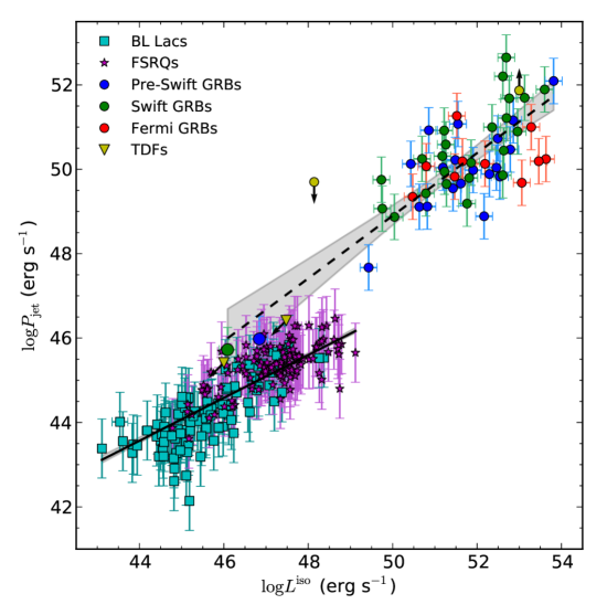
Figure 1: The relation between the jet kinetic power and the isotropically-equivalent $\gamma$-ray luminosity for AGNs and GRBs. Error bars, $1\sigma$. We fitted the two populations separately using a symmetric least-squares method (orthogonal BCES with bootstrapping; ?). The blazar and GRB best-fit models corresponds to the solid and dashed lines, respectively ($\log P_{\rm jet}=A\log L^{\rm iso}+B$). The best-fit parameters obtained for the blazars are $A=0.51\pm 0.02$ and $B=21.2\pm 1.1$; for the GRBs, $A=0.74\pm 0.08$ and $B=11.8\pm 4.1$. The scatter about the best-fit is 0.5 dex and 0.8 dex for the blazars and GRBs, respectively. The $2\sigma$ confidence band of the fits is shown as the gray shaded regions (barely visible for blazars). The two correlations do not agree at $>5\sigma$ level. We also include for illustration XRF 020903 and GRB 090423 (yellow circles) as well as the two recent tidal disruption flares (TDFs) detected with Swift which are presumably due to the onset of relativistic jets from the tidal disruption of stars by supermassive black holes  (?). We do not consider these sources in the statistics since we only have limits on their luminosities

.

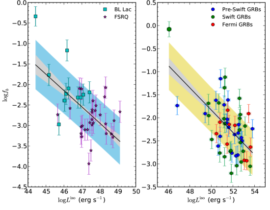
Figure 2: The relation between the apparent $\gamma$-ray luminosity and the beaming factor for blazars (left panel) and GRBs (right panel). We find $r=-0.53$ and $-0.56$ for blazars and GRBs, respectively, indicating anti correlations significant at the $3.6\sigma$ and $4.4\sigma$ levels respectively. The solid lines correspond to the best-fit linear models obtained with the symmetric least-squares fit and are given by $f_{b}\approx 5\times 10^{-4}(L_{49}^{\rm iso})^{-0.39\pm 0.15}$ and $\approx 0.03(L_{49}^{\rm iso})^{-0.24\pm 0.06}$ for blazars and GRBs, respectively. The gray shaded region corresponds to the $1\sigma$ confidence band and the blue and yellow regions are the $1\sigma$ prediction bands, which quantify the scatter about the best-fits.

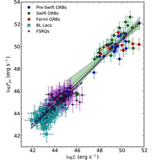
Figure 3: The relation between the collimation-corrected $\gamma$-ray luminosity $L=f_{b}L^{\rm iso}$ and the kinetic power for AGNs and GRBs. The shaded regions display the $2\sigma$ confidence band of the fits. The blazar and GRB best-fit models (dashed and dotted lines, respectively) follow correlations which are consistent, within the uncertainties, with the best-fit model obtained from the joint data set (solid line). In other words, using $L$ instead of $L^{\rm iso}$ leads to correlations for AGNs and GRBs which are consistent with each other (compare to Fig. 1). The best-fit parameters obtained from the combined data set are $\alpha=0.98\pm 0.02$ and $\beta=1.6\pm 0.9$ where $\log P_{\rm jet}=\alpha\log L+\beta$. The scatter about the best-fit is 0.64 dex. The yellow data points correspond to XRF 020903 and GRB 090423, which we do not take into account in the statistics.

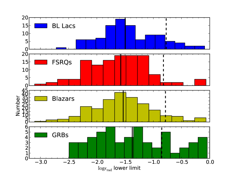
Figure 4: Distribution of the $1\sigma$ lower limits on the jet radiative efficiency (the fraction of the total jet power which is converted to $\gamma$-rays) $\epsilon_{\rm rad}\equiv L/(L+P_{\rm jet})$ for AGNs and GRBs. The vertical solid lines indicate the median values of the lower limits and the dashed lines represent the median values of $\epsilon_{\rm rad}$ for each sample. Most of the sources are characterized by $\epsilon_{\rm rad}>3\%$. The median efficiencies correspond to about $15\%$, keeping in mind that these estimates are affected by $\sim 0.5-0.7$ dex uncertainties on average.

Supplementary Materials

Data

Table S1 lists the properties of the 234 blazars in our sample (106 BL Lac objects and 128 FSRQs). Our sample includes the well-studied blazars OJ 287, 3C 454.3, 3C 279 and 3C 273. The redshifts were estimated as described in  (?).

Table S2 lists the corresponding properties of the 54 GRBs (49 long and 5 short). We include in our data the sub-energetic bursts GRB 031203  (?) and GRB 980425  (?). The latter one is associated with the nearby (distance $\sim$ 40 Mpc) supernova 1998bw  (?, ?). We also include in our sample the naked-eye GRB 080319B  (?). We include in Table S2 the X-ray flash (XRF) 020903  (?) and the most distant cosmic explosion ever detected, GRB 090423 at $z\approx 8.2$  (?, ?) but we do not take these GRBs into account in the statistics, since we have only limits on their collimation-corrected energetics.

Calculation of $\gamma$-ray luminosity and jet power

Blazars

$\gamma$-ray luminosity:

In order to calculate the total Fermi $\gamma$-ray luminosity, we follow a procedure similar to that of  (?) (their equation 1). The procedure to calculate the $k$-corrected band luminosity depends on the type of model used in the 2FGL analysis  (?, ?). In the case of a power law energy model, the total 100 MeV to 100 GeV $k$-corrected luminosity is calculated from the energy flux ($S_{\gamma}$) given in the catalog:

$$L^{\rm iso}=4\pi d_{L}^{2}\frac{S_{\gamma}}{(1+z)^{1-\alpha_{\gamma}}},$$ (1)

where $d_{L}$ is the luminosity distance in cm² and $\alpha_{\gamma}$ is the (energy) spectral slope over the whole band.

In the 2FGL catalog, some blazars are now modeled with the ’Log Parabolic’ form. The $k$-corrected energy flux in this case must be calculated numerically. The integral form is

$$S_{\gamma}^{\prime}=\chi\int_{E_{1}}^{E_{2}}K\left(\frac{E}{E_{0}(1+z)}\right)^{-\alpha-\beta\mathrm{log}\left(\frac{E}{E_{0}(1+z)}\right)}\left(1+z\right)^{-2}E\,dE,$$ (2)

where $E_{1}$ = 0.1 GeV and $E_{2}$ = 100 GeV and we have used the fit given in the 2FGL catalog for each source, with values $\alpha$ (column name ‘spectral_index’), $\beta$ (‘beta’), and $E_{0}$ (‘pivot_energy’), and K (‘flux_density’). The constant $\chi$ = 1.6 erg MeV GeV^-2 gives the energy flux in final units of erg cm^-2 s^-1.

The band luminosity for the Log-Parabolic model case can then be simply calculated from

$$L^{\rm iso}=4\pi d_{L}^{2}\,S_{\gamma}^{\prime}.$$ (3)

We calculate the uncertainty in $L^{\rm iso}$ propagating the error associated with $\alpha_{\gamma}$ and $S_{\gamma}$ quoted in the 2FGL. The average uncertainty in $L^{\rm iso}$ corresponds to 0.05 dex.

In order to estimate the uncertainty affecting the collimation-corrected luminosities $L$ we first evaluate the error in the beaming angle $\theta$ or correspondingly $\Gamma$. The uncertainty in $\Gamma$ is dominated by the uncertainty in the variability Doppler factor whereas the uncertainty in the apparent speed does not contribute significantly to the error budget of $\Gamma$. The uncertainty in the variability Doppler factor is $\approx 27\%$ (1 s.d.; ?). Therefore, for the blazars with direct estimates of $\Gamma$ available, the relative uncertainty in $\Gamma$ is $0.3$  (?, ?) which translates to an average uncertainty of 0.26 dex in $L$ for these blazars. For the blazars without direct estimates of $\Gamma$, we estimate the uncertainty in $L$ using the prediction band of the $L^{\rm iso}-f_{b}$ relation shown in Fig. 2. The plotted prediction band corresponds to a relative uncertainty of 0.69 in $\theta$. The resulting average uncertainty affecting $L$ for the blazars without direct estimates of $\Gamma$ is then 0.6 dex.

Kinetic power:

Following  (?), we estimate the jet kinetic power by using the correlation between the extended radio emission and the jet power  (?, ?). Cavagnolo et al. searched for X-ray cavities in different systems including giant elliptical galaxies and cD galaxies and estimated the jet power required to inflate these cavities or bubbles, obtaining the tight correlation

$$P_{\rm cav}\approx 6\times 10^{43}\left(\frac{P_{\rm radio}}{{10^{40}\ \rm erg\;s}^{-1}}\right)^{0.7}{{\rm erg\;s}^{-1}}$$ (4)

between the “cavity” power and the radio luminosity. Hence, assuming $P_{\rm jet}=P_{\rm cav}$ we can estimate the jet kinetic power for the blazars which have extended radio emission observed with the VLA  (?).

The uncertainty in $P_{\rm jet}$ is dominated by the scatter in the correlation of  (?) and corresponds to 0.7 dex.

GRBs

$\gamma$-ray luminosity:

The current scenario for GRBs  (?, ?) posits that initially most of the energy produced by the GRB is in kinetic form produced during the short “active” state of the stellar-mass central engine. A certain fraction of initial energy is converted after a few seconds mostly to $\gamma$-rays observed during the prompt emission, by means of internal shocks in the jet  (?). The ultrarelativistic jet produced in the explosion later on collides with the circumburst medium producing the afterglow. Two crucial quantities which we use in this work are the radiative and kinetic energies released by the GRBs during their short period of activity.

The isotropically equivalent energy radiated in $\gamma$-rays $E_{\gamma}^{\rm iso}$ is directly available from measurements. It was measured for the GRBs using a variety of different telescopes including pre-Swift telescopes (BeppoSAX, BATSE, HETE, HETE-2 and Integral) as well as Swift and Fermi (see Table S2). We calculate the isotropically-equivalent $\gamma$-ray luminosity as

$$L^{\rm iso}=\frac{(1+z)}{t_{90}}E_{\gamma}^{\rm iso}$$ (5)

where $t_{90}$ is the duration containing $90\%$ of the fluence in the observer frame.

The energy range in which the fluence is measured is typically $\sim 10$ keV – 10 MeV. Most of the radiative energy released in the GRB jet during the prompt emission is contained in this energy range according to the latest GRB SEDs observed  (?).

We adopt an uncertainty of 0.2 dex on the values of $E_{\gamma}^{\rm iso}$ which corresponds to the typical uncertainty affecting the GRBs in the sample studied by  (?). Therefore, the resulting uncertainty in the value of $L^{\rm iso}$ corresponds to 0.2 dex.

The collimation-corrected $\gamma$-ray luminosity is computed as

$$L=\frac{(1+z)}{t_{90}}f_{b}E_{\gamma}^{\rm iso}$$ (6)

where $f_{b}$ is the beaming factor ($f_{b}=1-\cos\theta_{\rm j}$) and $\theta_{\rm j}$ is the jet half-opening angle. This relies on the afterglow lightcurve displaying a jet break which is used to estimate $\theta$  (?). $\left\langle\theta_{\rm j}\right\rangle\approx 8^{\circ}$ for the sample and $\left\langle f_{b}\right\rangle\approx 9\times 10^{-3}$. We adopt an uncertainty of 0.1 dex on the values of $\theta_{\rm jet}$, which corresponds to the typical uncertainty in the values of $\theta_{\rm j}$ for the sample studied by  (?).

We calculated the uncertainty in $L$ using error propagation from the uncertainties in $E_{\gamma}^{\rm iso}$ and $\theta$, obtaining that the uncertainty in $L$ is $\approx 0.3$ dex.

Kinetic energy:

The jet kinetic energy is estimated from the radio or X-ray afterglow lightcurve using the fireball model  (?). For most of the GRBs, X-ray data were used to determine this energy  (?, ?). In a few cases, radio data were used  (?, ?, ?).

The standard fireball afterglow model depends on five model parameters: the explosion kinetic energy $E_{k}^{\rm iso}$, the density of the circumburst environment $n$ (with which the jet collides), the spectral index of the electron energy distribution $p$ and the fractions $\epsilon_{e}$ and $\epsilon_{B}$ of shock thermal energy carried by electrons and magnetic field, respectively. The typical values adopted for these parameters are $p=2.2$, $n=1\ {\rm cm}^{-3}$, $\epsilon_{e}=0.1$ and $\epsilon_{B}=0.01$ (e.g., ?, ?). The afterglow model relates the specific flux at a certain frequency and at a specific time after the burst (typically 10 hours in the observed frame) with the kinetic energy.

The measurement of $E_{k}^{\rm iso}$ can be impacted by the afterglow plateau which possibly corresponds to a late activity of the central engine. Indeed,  (?) demonstrated the impact of choosing two different times for the measurement of $E_{k}^{\rm iso}$: $t_{\rm dec}$ (deceleration time) or $t_{b}$ (injection break time). Adopting $t_{\rm dec}$ would lead to an underestimation of $E_{k}^{\rm iso}$ because this choice of time does not include the plateau.

The kinetic energy estimates we used in our analysis were computed at either $\sim 10$ h or $\sim 24$ h (cf. Table S2). We verified that these times are usually beyond the “break time” of the plateau reported in  (?). Therefore, the measurements of $E_{k}^{\rm iso}$ used in this paper correspond to conservative estimates. Moreover, the choice of the time at either $\sim 10$ h and $\sim 24$ h affects very little the measurement of $E_{k}^{\rm iso}$  (?).

The typical uncertainty in $E_{k}^{\rm iso}$ due to observational errors is $\approx 0.3$ dex  (?, ?). The value of $E_{k}^{\rm iso}$ is also sensitive to the values of parameters which regulate the microphysics of the fireball afterglow model and are poorly constrained. The systematic error affecting $E_{k}^{\rm iso}$ due to the uncertainties in the parameters $\epsilon_{e}$ and $\epsilon_{B}$ of the fireball afterglow model can be as high as 0.45 dex  (?, ?). Therefore, we combined the uncertainty resulting from the observational and systematic sources of errors in quadrature and conservatively adopt an uncertainty of 0.5 dex for $E_{k}^{\rm iso}$.

Kinetic power:

The jet kinetic power is computed as

$$P_{\rm jet}=\frac{(1+z)}{t_{90}}f_{b}E_{k}^{\rm iso}.$$ (7)

$L_{\gamma}^{iso}$ and $P_{\rm jet}$ should be thought as the average luminosities over the duration $t_{90}$ of the prompt emission phase, i.e. the average luminosities over the timescale during which the central engine is producing the jet. We calculated the uncertainty in $P_{\rm jet}$ using error propagation from the uncertainties in $E_{k}^{\rm iso}$ and $\theta$, obtaining that the uncertainty affecting $P_{\rm jet}$ is $\approx 0.54$ dex.

Linear regression method

Here we present more details about the linear regression method that we use in the paper.

We fitted the datasets using the BCES (bivariate correlated errors and intrinsic scatter) regression method  (?) which takes into account measurement errors in both the “$X$” and “$Y$” coordinates and the intrinsic scatter in the data. This method has been widely used in fitting datasets in the astronomical community  (?, ?).

It is not clear in the data sets analyzed in this work which quantities should be treated as the dependent variables and which ones should be treated as independent from a physical point of view. There is no a priori reason to expect the luminosity to be the independent variable as opposed to the kinetic power (or beaming factor). For this reason, we treat the variables symmetrically and adopt the BCES orthogonal regression method, which minimizes the squared orthogonal distances. Uncertainties on the parameters derived from the fits are estimated after carrying out 100000 bootstrap resamples of the data.

Partial correlation analysis

When studying correlations between luminosities one should be careful to take into account their common dependence on the distance  (?). We performed a partial correlation analysis of the common dependence of $L_{\gamma}^{\rm iso}$ and $P_{\rm jet}$ on the distance using the partial Kendall’s $\tau$ correlation test  (?).

We applied this test to our data considering $X=P_{\rm jet}$, $Y=L^{\rm iso}$ and $Z=\log d_{L}$. Table S3 lists the results of the partial correlation analysis. This test demonstrates that the $p$-value of the null hypothesis (i.e. no correlation between $X$ and $Y$) is $1.2\times 10^{-7}$ when considering the GRB subsample and $<10^{-10}$ when considering the blazar subsample or the combined blazar-GRB sample. Therefore, the $L^{\rm iso}-P_{\rm jet}$ correlation is strong and not a distance-driven artifact.

Objects	N	$\tau$	$\sigma$	$P_{\rm null}$	Signif. rejection null
Blazars	234	0.3	0.04	$5\times 10^{-15}$	7.8
GRBs	54	0.4	0.08	$1.6\times 10^{-7}$	5.2

Table S3 Results of partial correlation analysis with $X=P_{\rm jet}$, $Y=L^{\rm iso}$ and $Z=\log d_{L}$.
Notes. Column (1): subsample. Column (2): Number of sources. Column (3)-(6): results of partial correlation analysis; $\tau$ is the partial Kendall’s correlation coefficient; $\sigma$ is the square root of the calculated variance; $P_{\rm null}$ is the probability for accepting the null hypothesis that there is no correlation between $X$ and $Y$; Column (6) gives the associated significance in standard deviations with which the null hypothesis is rejected.

We then applied the partial correlation test to the data considering $X=P_{\rm jet}$, $Y=L$ and $Z=\log d_{L}$, i.e. we replaced the isotropically-equivalent luminosity in $Y$ with the collimation-corrected one. Table S4 lists the results of the analysis. This test demonstrates that the p-value of the null hypothesis is $\ll 10^{-10}$, $\approx 10^{-12}$ and $10^{-9}$ when considering the combined blazar-GRB sample, the blazars and the GRB, respectively. Hence, the $L-P_{\rm jet}$ correlation remains very strong after correcting for beaming.

Objects	N	$\tau$	$\sigma$	$P_{\rm null}$	Signif. rejection null
All objects	288	0.57	0.06	$\ll 10^{-10}$	9.4
Blazars	234	0.24	0.03	$2\times 10^{-12}$	7
GRBs	54	0.47	0.08	$10^{-9}$	6.1

Table S4 Same as Table S3 with $X=P_{\rm jet}$, $Y=L$ and $Z=\log d_{L}$.

Blazar luminosity estimates: Impact of the synchrotron peak

We discuss in this section the impact of the lower energy synchrotron peak – observed in the spectral energy distribution of blazars  (?, ?) – in estimating the jet radiative luminosity.

A subset of 131 blazars – roughly half of the original AGN sample – have adequate sampling of their multiwavelength spectral energy distributions which allow us to quantify the impact of the synchrotron peak in the estimate of the jet radiative luminosity. We estimated the bolometric luminosity as $L_{\rm bol}^{\rm iso}=L^{\rm iso}+L_{\rm syn}^{\rm iso}$ where $L_{\rm syn}^{\rm iso}$ is the isotropically-equivalent luminosity of the synchrotron peak. We obtained that the values of $L_{\rm bol}^{\rm iso}$ for the quasars are not much different from $L^{\rm iso}$ (on average by a factor of $\approx 1.7$), whereas the values of $L_{\rm bol}^{\rm iso}$ for the BL Lacs are somewhat different (on average by a factor of $\approx 2.8$).

We computed the intrinsic bolometric luminosity as $L_{\rm bol}=f_{b}L_{\rm bol}^{\rm iso}$, correcting $L_{\rm bol}^{\rm iso}$ for the opening angle or beaming factor. As previously discussed, estimates of $f_{b}$ for blazars rely on measurements of $\Gamma$ which are not available for all the blazars in our sample. For this reason, we use the anti correlation between $L_{\rm bol}^{\rm iso}$ and $f_{b}$ as an estimator of $f_{b}$ for the blazars without measurements of $\Gamma$.

We show in Figure S1 the resulting relation between $L_{\rm bol}$ and $P_{\rm jet}$ compared to the $L-P_{\rm jet}$ fit derived before (cf. Fig. 3). Figure S1 illustrates that the $L_{\rm bol}-P_{\rm jet}$ and $L-P_{\rm jet}$ best-fits are characterized by very similar slopes. However, the fit based on $L_{\rm bol}$ is characterized by slightly higher radiative efficiencies: for a given jet power, the jet luminosity is higher on average by a factor of $\approx 2$ compared to the fit based on $L$. Therefore, the results based on $L_{\rm bol}$ strengthen our conclusion that AGN jets have high radiative efficiencies while still being in qualitative agreement with the GRB result.

Figure S1 The relation between the collimation-corrected bolometric luminosity $L_{\rm bol}$ and the kinetic power for the 131 blazars with measurements of synchrotron peak luminosity. The solid line in this figure corresponds to the fit based on $L_{\rm bol}$ whereas the dashed line is the fit based on $L$. The shaded regions display the $2\sigma$ confidence band of the fits. Error bars, $1\sigma$.

Table S1. Properties of the blazar sample.
2FGL name	Alias	Type	$z$	$\log L^{\rm iso}$	Unc.a	$\log L$	Unc.b	$\log P_{\rm jet}$c	$\log f_{b}$d
				(erg s-1)	$\log L^{\rm iso}$	(erg s-1)	$\log L$	(erg s-1)
J0757.1+0957	PKS 0754+100	BLL	0.266	45.72	0.04	42.75	0.26	44.34	-2.97*
J0811.4+0149	PKS 0808+019	BLL	1.148	47.13	0.05	44.56	0.57	45.18	-2.57
J0807.1-0543	PKS 0804-055	BLL	0.158	45.01	0.06	43.16	0.57	44.16	-1.84
J0808.2-0750	PKS 0805-07	FSRQ	1.837	48.61	0.02	45.53	0.56	45.96	-3.08
J0825.9+0308	PKS 0823+033	BLL	0.506	45.86	0.09	43.73	0.57	44.45	-2.14
J0831.9+0429	PKS 0829+046	BLL	0.174	45.68	0.02	43.6	0.56	44.18	-2.08
J0839.4+1802	BZB J0839+1802	BLL	0.28	45.17	0.1	43.27	0.57	44.58	-1.9
J0847.2+1134	BZB J0847+1133	BLL	0.199	44.98	0.12	43.14	0.58	43.76	-1.83
J0839.6+0059	PKS 0837+012	FSRQ	1.123	46.87	0.08	44.39	0.57	45.41	-2.49
J0303.5+4713	4C +47.08	BLL	0.475	46.3	0.04	44.01	0.57	44.71	-2.29
J0854.8+2005	OJ 287	BLL	0.306	46.12	0.03	43.89	0.26	44.17	-2.23*
J2151.5-3021	PKS 2149-307	FSRQ	2.345	48.48	0.06	45.44	0.57	45.67	-3.04
J2158.8-3013	PKS 2155-304	BLL	0.117	45.98	0.01	43.8	0.56	43.9	-2.18
J2258.0-2759	PKS 2255-282	FSRQ	0.927	47.35	0.03	44.7	0.57	45.35	-2.65
J0120.4-2700	0118-272	BLL	0.557	46.78	0.03	44.32	0.57	45.06	-2.45
J0252.7-2218	PKS 0250-225	FSRQ	1.427	48.02	0.03	45.14	0.57	45.5	-2.88
J2213.1-2527	PKS 2210-25	FSRQ	1.831	47.6	0.08	44.86	0.57	45.97	-2.73
J2243.2-2540	PKS 2240-260	BLL	0.774	46.81	0.04	44.35	0.57	45.33	-2.47
J0137.6-2430	PKS 0135-247	FSRQ	0.831	46.78	0.05	44.33	0.57	45.57	-2.45
J0205.3-1657	PKS 0202-17	FSRQ	1.74	47.77	0.06	44.98	0.57	45.42	-2.79
J2157.9-1501	PKS 2155-152	FSRQ	0.672	46.44	0.06	44.11	0.57	45.34	-2.34
J0132.8-1654	PKS 0130-17	FSRQ	1.02	47.35	0.03	44.7	0.57	45.22	-2.65
J2347.9-1629	PKS 2345-16	FSRQ	0.576	46.5	0.05	44.14	0.57	45.21	-2.36
J0116.0-1134	PKS 0113-118	FSRQ	0.672	46.71	0.03	44.28	0.57	45.46	-2.43
J2229.7-0832	PKS 2227-08	FSRQ	1.56	48.26	0.03	45.96	0.26	45.17	-2.3*
J0102.7+5827	TEX 0059+581	FSRQ	0.643	46.82	0.03	44.36	0.57	44.78	-2.47
J0050.6-0929	PKS 0048-09	BLL	0.2	45.7	0.03	43.62	0.56	44.31	-2.08
J0141.5-0928	0138-097	BLL	0.733	46.65	0.05	44.24	0.57	45.08	-2.41
J2225.6-0454	3C 446	FSRQ	1.404	47.74	0.03	45.11	0.26	46.29	-2.64*
J2133.8-0154	4C -02.81	BLL	1.285	47.18	0.07	44.59	0.57	45.67	-2.59
J2338.1-0229	PKS 2335-027	FSRQ	1.072	47.32	0.04	44.68	0.57	45.22	-2.64
J0108.6+0135	PKS 0106+01	FSRQ	2.099	48.64	0.02	45.43	0.26	46.46	-3.21*
J0217.9+0143	PKS 0215+015	FSRQ	1.715	48.18	0.02	45.24	0.56	45.79	-2.93
J2148.2+0659	4C +06.69	FSRQ	0.99	46.87	0.09	44.77	0.28	45.1	-2.1*
J2334.3+0734	BZQ J2334+0736	FSRQ	0.401	45.87	0.06	43.73	0.57	44.6	-2.14
J2330.2+1107	4C +10.73	FSRQ	1.489	47.34	0.12	44.7	0.58	45.4	-2.65
J0259.5+0740	0256+075	FSRQ	0.893	46.62	0.09	44.22	0.57	45.06	-2.4
J2147.3+0930	2144+092	FSRQ	1.113	47.72	0.02	44.95	0.56	45.46	-2.78
J2232.4+1143	4C 11.69	FSRQ	1.037	47.56	0.03	44.89	0.26	45.72	-2.68*
J2253.9+1609	3C 454.3	FSRQ	0.859	48.79	0.0	45.91	0.26	45.86	-2.88*
J2143.5+1743	S3 2141+17	FSRQ	0.211	46.01	0.01	43.82	0.56	44.38	-2.19
J2203.4+1726	PKS 2201+171	FSRQ	1.075	47.74	0.02	44.95	0.56	45.49	-2.78
J0238.7+1637	AO 0235+164	BLL	0.524	47.38	0.01	44.72	0.56	44.72	-2.66
J0112.1+2245	S2 0109+22	BLL	0.265	46.24	0.02	43.97	0.56	43.75	-2.27
J2217.1+2422	B2 2214+24B	BLL	0.505	46.06	0.06	43.85	0.57	44.78	-2.21
J2311.0+3425	B2 2308+34	FSRQ	1.817	48.2	0.03	45.26	0.57	45.79	-2.94
J0205.4+3211	0202+319	FSRQ	1.466	47.34	0.09	44.69	0.57	45.33	-2.65
J0237.8+2846	4C +28.07	FSRQ	1.207	47.78	0.03	45.27	0.26	45.59	-2.52*
J0221.0+3555	0218+357	FSRQ	0.96	47.56	0.02	44.84	0.56	45.58	-2.72
J0909.1+0121	4C +01.24	FSRQ	1.024	47.6	0.04	44.86	0.57	45.25	-2.74
J0915.8+2932	B2 0912+29	BLL	0.096	44.75	0.05	42.99	0.56	43.76	-1.76
J0927.9-2041	PKS 0925-203	FSRQ	0.348	45.63	0.07	43.57	0.57	44.8	-2.06
J0956.9+2516	OK 290	FSRQ	0.712	46.67	0.04	44.25	0.57	44.8	-2.41
J1014.1+2306	4C +23.24	FSRQ	0.565	46.07	0.09	43.86	0.57	45.35	-2.21
J1012.1+0631	BZB J1012+0630	BLL	0.727	46.3	0.09	44.01	0.57	45.32	-2.29
J1023.6+3947	B2 1020+40	FSRQ	1.254	47.02	0.08	44.48	0.57	45.78	-2.54
J1051.3+3938	BZB J1051+3943	BLL	0.49	45.57	0.17	43.53	0.59	43.93	-2.04
J1040.7+0614	4C +06.41	FSRQ	1.27	47.38	0.05	44.72	0.57	45.06	-2.66
J1058.4+0133	4C +01.28	BLL	0.888	47.42	0.02	45.23	0.26	45.61	-2.19*
J1104.4+3812	MKN 421	BLL	0.03	44.88	0.01	43.08	0.56	43.28	-1.8
J1121.0+4211	EXO 1118.0+4228	BLL	0.124	44.82	0.07	43.04	0.57	42.61	-1.78
J1132.9+0033	PKS 1130+008	BLL	1.223	47.32	0.05	44.68	0.57	45.46	-2.64
J1130.3-1448	PKS 1127-145	FSRQ	1.187	47.68	0.03	44.92	0.57	45.62	-2.76
J1126.6-1856	PKS 1124-186	FSRQ	1.048	47.52	0.02	44.81	0.56	45.2	-2.71
J1146.9+4000	S4 1144+402	FSRQ	1.088	47.34	0.03	44.69	0.57	44.56	-2.65
J1146.8-3812	PKS 1144-379	FSRQ	1.048	47.16	0.05	44.58	0.57	44.89	-2.58
J1159.5+2914	4C +29.45	FSRQ	0.729	47.31	0.02	44.21	0.26	45.43	-3.1*
J1209.6+4121	B3 1206+416	BLL	0.194	44.81	0.13	43.04	0.58	43.15	-1.78
J1206.0-2638	PKS 1203-26	FSRQ	0.786	46.79	0.06	44.33	0.57	45.7	-2.46
J1221.3+3010	PG 1218+304	BLL	0.2	45.61	0.05	43.56	0.57	44.49	-2.05
J1217.8+3006	ON 325	BLL	0.1	45.18	0.02	43.28	0.56	43.92	-1.9
J1221.4+2814	ON 231	BLL	0.1	45.18	0.02	43.28	0.56	42.14	-1.91
J1222.4+0413	PKS 1219+04	FSRQ	0.965	47.36	0.04	44.7	0.57	45.42	-2.65
J1219.7+0201	PKS 1217+02	FSRQ	0.24	45.14	0.11	43.25	0.57	44.43	-1.89
J1225.0+4335	B3 1222+438	BLL	1.87	47.46	0.1	44.77	0.57	45.74	-2.69
J1231.7+2848	B2 1229+29	BLL	1.0	47.3	0.04	44.67	0.57	45.22	-2.63
J1224.9+2122	4C +21.35	FSRQ	0.435	47.5	0.01	43.9	0.26	45.38	-3.61*
J1229.1+0202	3C 273	FSRQ	0.158	46.34	0.01	43.76	0.26	45.5	-2.58*
J1243.1+3627	Ton 116	BLL	0.112	44.89	0.06	43.09	0.57	43.72	-1.81
J1256.1-0547	3C 279	FSRQ	0.536	47.64	0.01	44.7	0.26	45.73	-2.94*
J1246.7-2546	PKS 1244-255	FSRQ	0.638	47.31	0.02	44.67	0.56	45.14	-2.64
J1309.4+4304	B3 1307+433	BLL	0.69	46.61	0.05	44.22	0.57	44.25	-2.4
J1310.6+3222	1308+326	FSRQ	0.997	47.56	0.03	44.58	0.26	45.37	-2.99*
J1326.8+2210	B2 1324+22	FSRQ	1.4	47.69	0.04	44.92	0.57	45.11	-2.77
J1332.0-0508	PKS 1329-049	FSRQ	2.15	48.7	0.03	45.59	0.57	45.74	-3.11
J1337.7-1257	PKS 1335-127	FSRQ	0.539	46.53	0.04	44.16	0.57	45.15	-2.37
J1354.7-1047	PKS 1352-104	FSRQ	0.332	45.93	0.04	43.77	0.57	44.84	-2.16
J1405.1+0405	PKS 1402+044	FSRQ	3.215	47.68	0.16	44.92	0.59	46.29	-2.76
J1419.4+3820	B3 1417+385	FSRQ	1.82	47.58	0.09	44.85	0.57	45.07	-2.73
J1418.1+2539	BZB J1417+2543	BLL	0.237	44.92	0.12	43.1	0.57	44.2	-1.81
J1427.0+2347	PG 1424+240	BLL	0.16	45.98	0.02	43.8	0.56	44.22	-2.18
J1440.3-1540	PKS 1437-153	BLL	0.244	45.1	0.1	43.22	0.57	44.59	-1.88
J1513.6-3233	CRATES J1513-3234	FSRQ	0.244	45.6	0.04	43.55	0.57	44.79	-2.05
J1517.7-2421	AP Lib	BLL	0.049	44.5	0.03	42.83	0.56	43.57	-1.67
J0136.9+4751	DA 55	FSRQ	0.859	47.57	0.02	44.95	0.26	44.78	-2.62*
J1512.8-0906	PKS 1510-089	FSRQ	0.36	47.44	0.01	44.51	0.26	44.93	-2.93*
J1733.1-1307	NRAO 530	FSRQ	0.902	47.39	0.04	43.45	0.26	45.72	-3.93*
J2025.6-0736	PKS 2022-077	FSRQ	1.388	48.27	0.02	45.31	0.56	45.9	-2.97
J1510.9-0545	4C -05.64	FSRQ	1.191	47.55	0.05	44.83	0.57	46.07	-2.72
J1512.2+0201	PKS 1509+022	FSRQ	0.222	45.48	0.04	43.47	0.57	44.77	-2.01
J1549.5+0237	PKS 1546+027	FSRQ	0.414	46.26	0.03	43.98	0.57	44.42	-2.27
J1728.2+0429	PKS 1725+044	FSRQ	0.293	45.78	0.05	43.67	0.57	44.18	-2.11
J0217.7+7353	S5 0212+73	FSRQ	2.367	48.32	0.07	46.25	0.27	45.01	-2.07*
J1550.7+0526	4C +05.64	FSRQ	1.422	47.33	0.07	44.69	0.57	45.79	-2.64
J1751.5+0938	OT 081	BLL	0.322	46.26	0.03	44.16	0.26	44.86	-2.1*
J1608.5+1029	4C +10.45	FSRQ	1.226	47.56	0.05	44.7	0.26	45.29	-2.85*
J2035.4+1058	PKS 2032+107	FSRQ	0.601	46.67	0.04	44.25	0.57	44.88	-2.42
J1504.3+1029	PKS 1502+106	FSRQ	1.839	49.12	0.01	46.45	0.26	45.65	-2.66*
J1553.5+1255	PKS 1551+130	FSRQ	1.29	47.78	0.03	44.98	0.57	45.52	-2.8
J0222.6+4302	3C 66A	BLL	0.444	47.31	0.02	44.67	0.56	45.43	-2.64
J1838.7+4759	BZB J1838+4802	BLL	0.131	44.83	0.07	43.04	0.57	42.91	-1.78
J1540.4+1438	4C +14.60	BLL	0.605	46.04	0.1	43.65	0.28	45.26	-2.39*
J1607.0+1552	PKS 1604+159	BLL	0.357	46.06	0.03	43.86	0.57	44.82	-2.21
J1719.3+1744	PKS 1717+177	BLL	0.137	45.11	0.05	43.23	0.57	43.55	-1.88
J2009.7+7225	4C +72.28	BLL	0.156	45.08	0.04	43.21	0.57	44.35	-1.87
J1516.9+1925	PKS 1514+197	BLL	0.65	46.18	0.09	43.93	0.57	44.06	-2.25
J1746.0+2316	BZQ J1745+2252	FSRQ	1.884	47.73	0.11	44.95	0.58	45.53	-2.78
J1813.5+3143	B2 1811+31	BLL	0.117	44.85	0.04	43.06	0.56	43.62	-1.79
J1613.4+3409	OS 319	FSRQ	1.401	46.98	0.1	44.88	0.28	45.3	-2.11*
J2004.5+7754	S5 2007+777	BLL	0.342	45.71	0.05	43.62	0.57	44.33	-2.09
J1640.7+3945	NRAO 512	FSRQ	1.66	48.12	0.04	45.2	0.57	45.51	-2.91
J1635.2+3810	4C +38.41	FSRQ	1.814	48.72	0.02	45.44	0.26	45.62	-3.29*
J1642.9+3949	3C 345	FSRQ	0.593	46.95	0.04	43.75	0.26	45.74	-3.2*
J1653.9+3945	MKN 501	BLL	0.034	44.46	0.02	42.8	0.56	43.2	-1.66
J1749.1+4323	B3 1747+433	BLL	0.229	45.38	0.05	43.41	0.57	44.03	-1.97
J1801.7+4405	1800+440	FSRQ	0.663	46.33	0.08	44.03	0.57	45.25	-2.3
J0533.0+4823	TEX 0529+483	FSRQ	1.162	47.53	0.03	44.82	0.57	45.25	-2.71
J0456.1-4613	PKS 0454-46	FSRQ	0.858	47.11	0.03	44.54	0.57	45.8	-2.57
J0449.4-4350	PKS 0447-439	BLL	0.107	45.58	0.02	43.54	0.56	43.86	-2.04
J1829.2+5402	BZB J1829+5402	BLL	0.181	44.85	0.08	43.06	0.57	43.81	-1.79
J1824.0+5650	4C +56.27	BLL	0.663	46.93	0.02	44.61	0.26	45.4	-2.32*
J1806.7+6948	3C 371	BLL	0.051	44.42	0.02	44.08	0.24	43.95	-0.34*
J1800.5+7829	S5 1803+784	BLL	0.684	47.08	0.02	44.83	0.26	44.88	-2.25*
J0635.5-7516	PKS 0637-75	FSRQ	0.651	46.89	0.03	44.4	0.56	45.98	-2.49
J1118.1-4629	PKS 1116-46	FSRQ	0.713	46.53	0.07	44.16	0.57	45.83	-2.37
J1742.1+5948	RGB 1742+597	BLL	0.148	44.56	0.08	42.87	0.57	43.38	-1.69
J2202.8+4216	BL Lac	BLL	0.069	45.16	0.01	43.4	0.26	43.45	-1.77*
J1748.8+7006	1749+701	BLL	0.77	46.82	0.04	44.36	0.57	44.85	-2.47
J2258.8-5524	BZB J2258-5525	BLL	0.479	45.54	0.15	43.52	0.58	44.27	-2.03
J1740.2+5212	4C +51.37	FSRQ	1.375	47.83	0.03	45.01	0.57	45.37	-2.81
J1725.2+5853	BZB J1725+5851	BLL	0.125	44.41	0.08	42.77	0.57	43.67	-1.64
J1538.1+8159	1ES 1544+820	BLL	0.138	44.53	0.12	42.85	0.58	43.72	-1.68
J1428.0-4206	PKS 1424-41	FSRQ	1.522	48.43	0.02	45.41	0.56	46.29	-3.02
J0930.4+8611	S5 0916+864	BLL	0.217	45.2	0.06	43.29	0.57	43.8	-1.91
J2056.2-4715	PKS 2052-47	FSRQ	1.489	48.33	0.02	45.34	0.56	46.26	-2.99
J2139.3-4236	MH 2136-428	BLL	0.092	45.11	0.02	43.23	0.56	42.74	-1.88
J0641.2+7315	S5 0633+73	FSRQ	1.85	47.53	0.08	44.82	0.57	45.86	-2.71
J1727.1+4531	S4 1726+45	FSRQ	0.714	46.89	0.03	44.4	0.56	45.09	-2.49
J1728.2+5015	IZW 187	BLL	0.055	43.83	0.08	42.39	0.57	43.28	-1.44
J1700.2+6831	BZQ J1700+6830	FSRQ	0.301	46.2	0.02	43.95	0.56	44.37	-2.25
J0721.9+7120	S5 0716+714	BLL	0.3	46.78	0.01	44.46	0.26	44.76	-2.32*
J0710.5+5908	EXO 0706.1+5913	BLL	0.125	44.7	0.09	42.96	0.57	43.8	-1.74
J0654.5+5043	CRATES J0654+5042	FSRQ	0.135	45.17	0.03	43.27	0.56	43.62	-1.9
J0841.6+7052	4C +71.07	FSRQ	2.172	48.36	0.05	45.16	0.26	45.97	-3.2*
J0654.2+4514	S4 0650+45	FSRQ	0.933	47.34	0.03	44.7	0.56	45.1	-2.65
J0747.7+4501	B3 0745+453	FSRQ	0.192	44.78	0.1	43.02	0.57	43.87	-1.77
J0830.5+2407	B2 0827+24	FSRQ	0.941	47.17	0.04	44.07	0.26	45.22	-3.1*
J1017.0+3531	B2 1015+35B	FSRQ	1.228	47.04	0.11	44.5	0.57	45.23	-2.54
J1033.2+4117	S4 1030+415	FSRQ	1.117	47.18	0.04	44.59	0.57	45.35	-2.59
J1153.2+4935	SBS 1150+497	FSRQ	0.334	45.69	0.05	43.61	0.57	45.19	-2.08
J0710.8+4733	S4 0707+476	BLL	1.292	47.25	0.06	44.64	0.57	45.59	-2.62
J1637.7+4714	4C +47.44	FSRQ	0.74	46.88	0.03	44.39	0.57	45.42	-2.49
J1559.0+5627	BZB J1558+5625	BLL	0.3	45.62	0.05	43.56	0.57	44.3	-2.05
J1542.9+6129	BZB J1542+6129	BLL	0.124	45.45	0.02	43.45	0.56	43.19	-2.0
J1110.2+7134	BZB J1110+7133	BLL	0.201	44.61	0.12	42.9	0.58	43.82	-1.71
J0816.5+5739	SBS 0812+578	BLL	0.226	45.21	0.07	43.3	0.57	44.01	-1.91
J1136.7+7009	MKN 180	BLL	0.046	43.85	0.06	42.4	0.56	43.48	-1.45
J1031.0+5053	1ES 1028+511	BLL	0.36	45.76	0.07	43.66	0.57	43.57	-2.1
J0958.6+6533	S4 0954+658	BLL	0.368	45.98	0.03	43.8	0.56	44.42	-2.18
J0921.9+6216	S4 0917+62	FSRQ	1.446	47.41	0.06	44.74	0.57	45.66	-2.67
J0809.8+5218	1ES 0806+524	BLL	0.138	45.14	0.04	43.25	0.56	43.29	-1.89
J1033.9+6050	S4 1030+61	FSRQ	1.401	47.87	0.02	45.04	0.56	45.51	-2.83
J0945.9+5751	BZB J0945+5757	BLL	0.229	45.0	0.07	43.16	0.57	43.82	-1.84
J1420.2+5422	1418+546	BLL	0.151	44.8	0.05	43.02	0.57	43.79	-1.77
J1154.4+6019	CRATES J1154+6022	FSRQ	0.543	46.19	0.06	43.94	0.57	44.51	-2.25
J1019.0+5915	BZB J1018+5911	BLL	0.191	44.6	0.1	42.9	0.57	43.74	-1.71
J0957.7+5522	4C +55.17	FSRQ	0.895	47.7	0.02	44.93	0.56	45.56	-2.77
J1248.2+5820	PG 1246+586	BLL	0.847	47.2	0.03	44.6	0.57	44.5	-2.6
J1151.5+5857	BZB J1151+5859	BLL	0.127	44.59	0.08	42.89	0.57	43.9	-1.7
J1058.6+5628	BZB J1058+5628	BLL	0.144	45.47	0.03	43.47	0.56	43.68	-2.0
J1037.6+5712	BZB J1037+5711	BLL	0.106	44.97	0.04	43.14	0.56	43.34	-1.83
J0929.5+5009	BZB J0929+5013	BLL	0.37	45.57	0.08	43.53	0.57	44.1	-2.04
J0818.2+4223	S4 0814+425	BLL	0.245	46.17	0.02	45.01	0.26	44.41	-1.17*
J1253.1+5302	S4 1250+53	BLL	0.204	45.69	0.03	43.61	0.56	44.17	-2.08
J0903.4+4651	S4 0859+470	FSRQ	1.462	46.95	0.11	44.44	0.58	46.1	-2.51
J0834.3+4221	S4 0830+42	FSRQ	0.249	45.24	0.07	43.32	0.57	44.18	-1.93
J0920.9+4441	S4 0917+44	FSRQ	2.189	48.72	0.02	45.6	0.56	45.84	-3.12
J1439.2+3932	PG 1437+398	BLL	0.349	45.31	0.13	43.36	0.58	44.26	-1.95
J1012.5+4227	BZB J1012+4229	BLL	0.364	45.27	0.13	43.34	0.58	44.15	-1.94
J0948.8+4040	4C +40.24	FSRQ	1.252	46.98	0.09	43.71	0.28	45.65	-3.28*
J0917.0+3900	S4 0913+391	FSRQ	1.269	46.95	0.1	44.44	0.57	45.73	-2.51
J0337.0+3200c	NRAO 140	FSRQ	1.258	47.44	0.07	44.76	0.57	45.54	-2.68
J0339.4-0144	PKS 0336-019	FSRQ	0.852	46.96	0.04	43.93	0.26	45.31	-3.03*
J0340.6-2113	PKS 0338-214	BLL	0.048	43.61	0.07	42.24	0.57	43.56	-1.37
J0405.8-1309	PKS 0403-13	FSRQ	0.571	45.95	0.1	43.78	0.57	45.68	-2.17
J0424.7+0034	PKS 0422+004	BLL	0.31	45.88	0.04	43.73	0.57	43.88	-2.14
J0423.2-0120	PKS 0420-01	FSRQ	0.915	47.62	0.02	45.22	0.26	45.24	-2.4*
J0428.6-3756	PKS 0426-380	BLL	1.11	48.37	0.01	45.37	0.56	45.53	-3.0
J0448.9+1121	0446+112	FSRQ	1.207	47.73	0.03	44.95	0.57	45.22	-2.78
J0442.7-0017	PKS 0440-00	FSRQ	0.844	47.57	0.01	44.84	0.56	45.41	-2.72
J0501.2-0155	4C -02.19	FSRQ	2.286	48.02	0.07	45.28	0.27	46.3	-2.74*
J0505.5+0501	PKS 0502+049	FSRQ	0.954	46.99	0.07	44.46	0.57	45.16	-2.53
J0530.8+1333	PKS 0528+134	FSRQ	2.07	48.32	0.05	45.36	0.27	45.92	-2.96*
J0532.7+0733	TEX 0529+075	FSRQ	1.254	47.78	0.03	44.98	0.57	45.57	-2.8
J0538.8-4405	PKS 0537-441	BLL	0.896	48.25	0.01	45.29	0.56	45.53	-2.96
J0608.0-0836	OH -10	FSRQ	0.872	47.03	0.05	44.02	0.27	45.42	-3.01*
J0738.0+1742	PKS 0735+17	BLL	0.424	46.57	0.02	44.19	0.56	44.47	-2.38
J0739.2+0138	PKS 0736+01	FSRQ	0.191	45.65	0.02	42.91	0.26	44.1	-2.74*
J0730.2-1141	PKS 0727-11	FSRQ	1.591	48.75	0.01	45.62	0.56	44.8	-3.13
J0849.0+0455	BZB J0849+0455	BLL	1.07	46.6	0.14	44.21	0.58	45.37	-2.39
J2319.1-4208	PKS 2316-423	BLL	0.056	43.54	0.19	42.2	0.59	44.02	-1.34
J2204.6+0442	PKS 2201+04	BLL	0.028	43.11	0.08	41.91	0.56	43.38	-1.2
J2159.9+1023	CRATES J2200+1030	BLL	0.172	44.62	0.12	42.91	0.57	44.23	-1.71
J0250.6+1713	BZQ J0250+1712	FSRQ	0.207	45.13	0.08	43.25	0.57	44.25	-1.89
J0112.8+3208	NRAO 62	FSRQ	0.603	46.99	0.02	44.46	0.56	45.21	-2.52
J0909.7-0229	PKS 0907-023	FSRQ	0.957	47.13	0.04	44.55	0.57	45.3	-2.57
J0912.9-2102	BZB J0913-2103	BLL	0.198	45.01	0.09	43.16	0.57	44.45	-1.84
J1204.3-0711	BZB J1204-0710	BLL	0.185	44.91	0.08	43.1	0.57	43.84	-1.81
J1317.9+3426	B2 1315+34A	FSRQ	1.05	46.53	0.12	44.16	0.58	45.55	-2.37
J1312.4-2157	PKS 1309-216	BLL	1.489	47.55	0.05	44.83	0.57	45.84	-2.72
J1351.1+0032	PKS 1348+007	FSRQ	2.084	47.64	0.08	44.89	0.57	45.96	-2.75
J1435.1+2022	CRATES J1435+2021	BLL	0.227	45.01	0.09	43.16	0.57	44.61	-1.84
J1744.1+1934	1ES 1741+196	BLL	0.083	44.18	0.12	42.62	0.57	43.81	-1.56
J1849.4+6706	4C +66.20	FSRQ	0.657	47.25	0.02	44.63	0.56	45.39	-2.61
J0611.8-6059	BZQ J0610-6058	FSRQ	0.617	46.1	0.09	43.88	0.57	45.17	-2.22
J1219.2+7107	S5 1217+71	FSRQ	0.451	45.55	0.09	43.52	0.57	44.66	-2.03
J1136.3+6736	BZB J1136+6737	BLL	0.135	44.58	0.1	42.88	0.57	43.54	-1.7
J1454.4+5123	BZB J1454+5124	BLL	1.083	47.17	0.05	44.58	0.57	45.27	-2.59
J1203.2+6030	SBS 1200+608	BLL	0.066	43.95	0.07	42.47	0.57	43.45	-1.48
J1053.6+4928	BZB J1053+4929	BLL	0.14	44.77	0.08	43.01	0.57	43.68	-1.76
J1433.8+4205	B3 1432+422	FSRQ	1.24	46.85	0.09	44.37	0.57	45.34	-2.48
J0315.8-1024	PKS 0313-107	FSRQ	0.335	45.52	0.08	43.5	0.57	44.88	-2.02
J0612.8+4122	S4 0609+41	BLL	0.097	44.98	0.03	43.14	0.56	43.74	-1.83
J0630.9-2406	BZB J0630-2406	BLL	0.062	44.57	0.04	42.88	0.56	43.2	-1.69
Notes:
(a) Uncertainty on $L^{\rm iso}$ in dex.
(b) Uncertainty on the collimation-corrected $\gamma$-ray luminosity $L$ in dex.
(c) The uncertainty on $P_{\rm jet}$ is 0.7 dex as described in the text.
(d) Values with a “*” correspond to those measured by ?, otherwise they were estimated from the best-fit in Fig. 2.

Table S2. Properties of the GRB sample.
Name	$z$	$t_{90}$	$\theta_{j}$ a	$\log E_{\gamma}^{\rm iso}$ b	$\log L^{\rm iso}$ b	$\log L$c	$\log E_{k}^{\rm iso}$ d	$\log P_{\rm jet}$e	Observatory	Ref.
		(s)	(∘)	(erg)	(erg s-1)	(erg s-1)	(erg)	(erg s-1)
090323	3.57	133.1	2.8	54.53	53.06	50.14	54.07	49.68	LAT	1
090328	0.74	57.0	4.2	52.99	51.47	48.9	53.91	49.83	LAT	1
090902B	1.82	21.0	3.9	54.5	53.63	51.0	53.75	50.24	LAT	1
090926A	2.11	20.0	9.0	54.27	53.46	51.55	52.91	50.19	LAT	1
081222	2.77	5.8	2.8	53.47	53.28	50.35	54.12	51.0	GBM	2
090424	0.54	20.2	9.8	52.64	51.52	49.69	54.22	51.26	GBM	2
090618	0.54	24.0	6.7	53.38	52.19	50.02	53.49	50.13	GBM	2
091020	1.71	65.0	6.9	53.03	51.65	49.51	53.71	50.19	GBM	2
091127	0.48	68.7	5.5	52.14	50.47	48.13	53.36	49.35	GBM	2
091208B	1.06	71.0	7.3	52.33	50.8	48.7	53.7	50.07	GBM	2
970228	0.7	56.0	4.0	52.15	50.63	48.02	53.24	49.11	BeppoSAX	3,4,5,22
970508	0.84	14.0	21.6	51.74	50.86	49.71	52.96	50.92	BATSE	3,4,5,22
970828	0.96	160.0	7.1	53.34	51.43	49.32	53.57	49.55	BATSE	3,4,5,22
971214	3.42	30.0	5.5	53.32	52.49	50.16	53.89	50.73	BATSE	3,4,5,22
980613	1.1	42.0	12.6	51.73	50.43	48.81	53.05	50.13	BeppoSAX	3,4,5,22
980425	0.01	23.3	11.0	48.2	46.84	45.1	49.08	45.98	BeppoSAX	10,8,6
980703	0.97	76.0	11.2	52.78	51.19	49.47	53.35	50.04	BATSE	3,4,5,22
990123	1.6	61.0	4.9	54.16	52.79	50.36	54.27	50.47	BATSE	3,4,5,22
990510	1.62	57.0	3.4	53.25	51.91	49.14	54.08	49.98	BATSE	3,4,5,22
990705	0.84	32.0	5.3	53.41	52.17	49.8	52.49	48.89	BATSE	3,4,5,22
991216	1.02	15.0	4.6	53.73	52.86	50.36	54.53	51.16	BATSE	3,4,5,22
021004	0.85	9.0	6.8	53.23	52.54	50.39	52.66	49.83	BeppoSAX	3,4,5,22
000926	2.04	1.3	6.2	53.45	53.82	51.58	53.96	52.09	BeppoSAX	3,4,5,22
010222	1.48	74.0	3.2	53.93	52.46	49.65	54.32	50.04	BeppoSAX	3,4,5,22
011211	2.14	51.0	6.4	52.83	51.62	49.41	53.08	49.66	BeppoSAX	3,4,5,22
020405	0.7	40.0	7.8	52.86	51.49	49.45	53.63	50.22	BeppoSAX	3,4,5,22
020813	1.25	89.0	3.1	53.89	52.29	49.47	54.31	49.89	HETE	3,4,5,22
021004	2.32	52.4	12.7	52.75	51.55	49.93	53.89	51.07	HETE	3,4,5,22
031203	0.1	40.0	9.0	50.99	49.43	47.52	51.14	47.67	Integral	9,6
030329	0.17	22.3	5.1	52.1	50.82	48.42	52.8	49.12	HETE	7,11
050709	0.16	0.1	17.2	50.0	51.22	49.87	51.05	50.92	BAT	12
050820A	2.62	26.0	6.6	53.98	53.13	50.95	54.73	51.69	BAT	13,14
050904	6.3	225.0	8.0	54.12	52.63	50.62	53.95	50.45	BAT	13,15
060218	0.03	2100.0	80.4	49.4	46.09	46.01	49.11	45.73	BAT	16,23
060418	1.49	52.0	22.5	52.6	51.28	50.16	52.09	49.65	BAT	13
070125	1.55	60.0	13.2	53.98	52.61	51.03	52.81	49.86	BAT	13,17,18
080319B	0.94	50.0	7.0	52.67	51.26	49.13	54.13	50.59	BAT	21,13
050505	4.27	136.0	2.0	53.27	51.86	48.66	54.77	50.16	BAT	2
050814	5.3	48.0	2.4	53.24	52.36	49.32	54.92	51.0	BAT	2
051109A	2.35	360.0	3.4	52.82	50.79	48.02	54.23	49.43	BAT	2
051221A	0.55	8.0	11.8	51.41	50.7	49.02	52.64	50.25	BAT	2
060124	2.3	3.3	2.4	53.6	53.6	50.55	54.94	51.89	BAT	2
060614	0.12	6.9	11.6	50.52	49.73	48.05	52.23	49.75	BAT	2
060707	3.42	210.0	7.9	52.85	51.18	49.16	54.01	50.31	BAT	2
060814	0.84	1.2	3.5	52.78	52.96	50.24	53.44	50.9	BAT	2
061021	0.35	79.0	8.6	51.52	49.75	47.8	52.79	49.07	BAT	2
061222A	2.09	16.0	2.7	53.48	52.76	49.8	55.36	51.68	BAT	2
070306	1.5	3.0	4.4	52.78	52.7	50.16	53.83	51.21	BAT	2
070318	0.84	0.4	8.8	52.03	52.69	50.76	53.92	52.65	BAT	2
070508	0.82	23.4	3.5	52.87	51.76	49.03	53.03	49.19	BAT	2
080310	2.43	32.0	3.6	52.78	51.81	49.1	53.47	49.79	BAT	2
080413B	1.1	1.0	6.0	52.29	52.61	50.35	54.14	52.2	BAT	2
090313	3.38	170.0	3.1	52.82	51.23	48.38	54.38	49.94	BAT	2
091018	0.97	106.5	4.7	51.77	50.04	47.57	53.08	48.87	BAT	2
090423f	8.2	10.3	$>12$	53	53	$>51.3$	53.6	$>51.9$	BAT	19,20
020903g	0.251	10	$<90$	49.04	48.14	$<48.14$	50.6	$<49.7$	HETE-2	24,25
Notes:
(a) Uncertainty of 0.1 dex as described in the text.
(b) Uncertainty of 0.2 dex as described in the text.
(c) Uncertainty of 0.3 dex as derived from uncertainties in $\theta_{j}$ and $E_{\gamma}^{\rm iso}$.
(d) Uncertainty of 0.5 dex as described in the text.
(e) Uncertainty of 0.54 dex as derived from uncertainties in $\theta_{j}$ and $E_{k}^{\rm iso}$.
(f) Lower limit on the opening angle. Not taken into account in the statistics.
(g) X-ray flash with an upper limit on the opening angle. Not taken into account in the statistics.
References: 1. Cenko et al. 2012  (?), 2. Racusin et al. 2011  (?), 3. Bloom et al. 2003  (?),
4. Berger et al. 2003  (?), 5. Lloyd-Ronning & Zhang 2004  (?), 6. Ghisellini et al. 2006  (?),
7. Berger et al. 2003b  (?), 8. Li & Chevalier 1999  (?), 9. Soderberg et al. 2004  (?),
10. Yamasaki et al. 2003  (?), 11. Vanderspek et al. 2004  (?), 12. Villasenor et al. 2005  (?),
13. Cenko et al. 2010  (?), 14. Cenko et al. 2006  (?), 15. Kawai et al. 2006  (?),
16. Campana et al. 2006  (?), 17. Racusin et al. 2007  (?), 18. Bellm et al. 2008  (?),
19. Tanvir et al. 2009  (?), 20. Chandra 2010  (?), 21. Racusin et al. 2008  (?),
22. Fan & Piran 2006  (?), 23. Soderberg et al. 2006  (?), 24. Soderberg et al. 2004b  (?),
25. Sakamoto et al. 2004  (?).

References and Notes

- 1. Gehrels, N., Ramirez-Ruiz, E., & Fox, D. B. Ann. Rev. Astron. Astrophys. 47, 567 (2009).
- 2. Piran, T. Rev. of Mod. Phys. 76, 1143 (2004).
- 3. Mirabel I. F., & Rodriguez L. F. Annu. Rev. Astron. Astrophys. 37, 409 (1999).
- 4. Rees, M. J. Ann. Rev. Astron. Astrophys. 22, 471 (1984).
- 5. Krolik, J. H. Active galactic nuclei : from the central black hole to the galactic environment (Princeton University Press) (1999).
- 6. Meier, D. L., Koide, S. K., & Uchida, Y. Science 291, 84 (2001).
- 7. Narayan, R., & Quataert, E. Science 307, 77 (2005).
- 8. McNamara, B., & Nulsen, P. E. J. Ann. Rev. Astron. Astrophys. 45, 117 (2007).
- 9. Sijacki, D., Springel, V., & Hernquist, L. Mon. Not. R. Astron. Soc. 380, 877 (2007).
- 10. Marscher, A. P., et al. Nature 417, 625 (2002).
- 11. Merloni, A., Heinz, S., & Di Matteo, T. Mon. Not. R. Astron. Soc. 345, 1057 (2003).
- 12. Falcke, H., Körding, E., & Markoff, S. Astron. Astrophys. 414, 895 (2004).
- 13. Wang, J., & Wei, J. Astrophys. J. 726, L24 (2011).
- 14. Wu, Q., et al. Astrophys. J. 740, L21 (2011).
- 15. Ulrich, M., Maraschi, L., & Urry, C. M. Annu. Rev. Astron. Astrophys. 35, 445 (1997).
- 16. Fermi LAT Collaboration. Astrophys. J. 743, 171 (2011).
- 17. Meyer, E. T., Fossati, G., Georganopoulos, M., & Lister, M. L. Astrophys. J. 740, 98 (2011).
- 18. Cavagnolo, K. W., et al. Astrophys. J. 720, 1066 (2010).
- 19. Freedman, D. L., & Waxman, E. Astrophys. J. 547, 922 (2001).
- 20. See supplementary online material for more details.
- 21. Akritas, M. G., & Siebert, J. Astrophys. J. 470, 706 (1996).
- 22. Frail, D. A., et al. Astrophys. J. , 562, L55 (2001).
- 23. Jorstad, S. G., et al. Astrophys. J. 130, 1418 (2005).
- 24. Pushkarev, A. B., Kovalev, Y. Y., Lister, M. L., & Savolainen, T. Astron. Astrophys. 507, L33 (2009).
- 25. Celotti, A., & Fabian, A. Mon. Not. R. Astron. Soc. , 264, 228 (1993).
- 26. Yuan, F., Yu, Zhaolong, & Ho, L. C. Astrophys. J. , 703, 1034 (2009).
- 27. Celotti, A., & Ghisellini, G. Mon. Not. R. Astron. Soc. , 385, 283 (2008). celotti08
- 28. Ghisellini, G., Tavecchio, F., Foschini, L., Ghirlanda, G., Maraschi, L., & Celotti, A. Mon. Not. R. Astron. Soc. , 402, 497 (2010).
- 29. Fan, Y., & Piran, T. Mon. Not. R. Astron. Soc. , 369, 197 (2006).
- 30. Zhang, B., et al. Astrophys. J. , 655, 989 (2007).
- 31. Racusin, J. L., et al. Astrophys. J. 738, 138 (2011).
- 32. Sironi, L., & Spitkovsky, A. Astrophys. J. , 726, 75 (2009).
- 33. Bloom, J. S., et al. Science 333, 203 (2011).
- 34. Burrows, D. N., et al. Nature 476, 421 (2011).
- 35. Cenko, S. B., et al. Astrophys. J. 753, 77 (2012).
- 36. In order to include the TDFs in Figure 1, we used the Fermi LAT upper limit (?) observed for Swift J164449.3+573451 and we assumed for Swift J2058.4+0516 (?) where is the observed X-ray luminosity. We assumed where is the Eddington luminosity based on the black hole masses estimated by ?, ?, ?. These luminosities and powers should be treated as upper limits. Acknowledgements: We thank J. Racusin, M. Lister, C. Dermer, A. Pushkarev, J. McEnery, D. Donato, D. Kazanas, T. Nelson and F. Tombesi for crucial discussions. RSN and SG were supported by an appointment to the NASA Postdoctoral Program at Goddard Space Flight Center, administered by Oak Ridge Associated Universities through a contract with NASA. This research has made use of: (i) StatCodes statistical software hosted by Penn State’s Center for Astrostatistics; (ii) data obtained from the HETE science team via the website http://space.mit.edu/HETE/Bursts/Data. HETE is an international mission of the NASA Explorer program, run by the Massachusetts Institute of Technology; (iii) NASA/IPAC Extragalactic Database (NED) which is operated by the Jet Propulsion Laboratory, California Institute of Technology, under contract with the National Aeronautics and Space Administration.

References and Notes

- 1. Gehrels, N., Ramirez-Ruiz, E., & Fox, D. B. Ann. Rev. Astron. Astrophys. 47, 567 (2009).
- 2. Piran, T. Rev. of Mod. Phys. 76, 1143 (2004).
- 3. Mirabel I. F., & Rodriguez L. F. Annu. Rev. Astron. Astrophys. 37, 409 (1999).
- 4. Rees, M. J. Ann. Rev. Astron. Astrophys. 22, 471 (1984).
- 5. Krolik, J. H. Active galactic nuclei : from the central black hole to the galactic environment (Princeton University Press) (1999).
- 6. Meier, D. L., Koide, S. K., & Uchida, Y. Science 291, 84 (2001).
- 7. Narayan, R., & Quataert, E. Science 307, 77 (2005).
- 8. McNamara, B., & Nulsen, P. E. J. Ann. Rev. Astron. Astrophys. 45, 117 (2007).
- 9. Sijacki, D., Springel, V., & Hernquist, L. Mon. Not. R. Astron. Soc. 380, 877 (2007).
- 10. Marscher, A. P., et al. Nature 417, 625 (2002).
- 11. Merloni, A., Heinz, S., & Di Matteo, T. Mon. Not. R. Astron. Soc. 345, 1057 (2003).
- 12. Falcke, H., Körding, E., & Markoff, S. Astron. Astrophys. 414, 895 (2004).
- 13. Wang, J., & Wei, J. Astrophys. J. 726, L24 (2011).
- 14. Wu, Q., et al. Astrophys. J. 740, L21 (2011).
- 15. Ulrich, M., Maraschi, L., & Urry, C. M. Annu. Rev. Astron. Astrophys. 35, 445 (1997).
- 16. Fermi LAT Collaboration. Astrophys. J. 743, 171 (2011).
- 17. Meyer, E. T., Fossati, G., Georganopoulos, M., & Lister, M. L. Astrophys. J. 740, 98 (2011).
- 18. Cavagnolo, K. W., et al. Astrophys. J. 720, 1066 (2010).
- 19. Freedman, D. L., & Waxman, E. Astrophys. J. 547, 922 (2001).
- 20. See supplementary online material for more details.
- 21. Akritas, M. G., & Siebert, J. Astrophys. J. 470, 706 (1996).
- 22. Frail, D. A., et al. Astrophys. J. , 562, L55 (2001).
- 23. Jorstad, S. G., et al. Astrophys. J. 130, 1418 (2005).
- 24. Pushkarev, A. B., Kovalev, Y. Y., Lister, M. L., & Savolainen, T. Astron. Astrophys. 507, L33 (2009).
- 25. Celotti, A., & Fabian, A. Mon. Not. R. Astron. Soc. , 264, 228 (1993).
- 26. Yuan, F., Yu, Zhaolong, & Ho, L. C. Astrophys. J. , 703, 1034 (2009).
- 27. Celotti, A., & Ghisellini, G. Mon. Not. R. Astron. Soc. , 385, 283 (2008).
- 28. Ghisellini, G., Tavecchio, F., Foschini, L., Ghirlanda, G., Maraschi, L., & Celotti, A. Mon. Not. R. Astron. Soc. , 402, 497 (2010).
- 29. Fan, Y., & Piran, T. Mon. Not. R. Astron. Soc. , 369, 197 (2006).
- 30. Zhang, B., et al. Astrophys. J. , 655, 989 (2007).
- 31. Racusin, J. L., et al. Astrophys. J. 738, 138 (2011).
- 32. Sironi, L., & Spitkovsky, A. Astrophys. J. , 726, 75 (2009).
- 33. Bloom, J. S., et al. Science 333, 203 (2011).
- 34. Burrows, D. N., et al. Nature 476, 421 (2011).
- 35. Cenko, S. B., et al. Astrophys. J. 753, 77 (2012).
- 36. In order to include the TDFs in Figure 1, we used the Fermi LAT upper limit (?) observed for Swift J164449.3+573451 and we assumed for Swift J2058.4+0516 (?) where is the X-ray luminosity. We assumed where is the Eddington luminosity based on the black hole masses estimated by ?, ?, ?. These luminosities and powers should be treated as upper limits.
- 37. Soderberg, A. N., et al. Nature 430, 648 (2004).
- 38. Pain, E., et al. Astrophys. J. 536, 778 (2000).
- 39. Galama, T. J., et al. Nature 395, 670 (1998).
- 40. Kulkarni, S. R., et al. Nature 395, 663 (1998).
- 41. Soderberg, A. M., et al. Astrophys. J. 606, 994 (2004b).
- 42. Racusin, J., et al. Nature 455, 183 (2008).
- 43. Tanvir, N. R., et al. Nature 461, 1255 (2009).
- 44. Chandra, P. Astrophys. J. , 712, L31 (2010).
- 45. Dainotti, M. G., et al. Astrophys. J. , 722, L215 (2010).
- 46. Ghisellini, G., Maraschi, L., & Tavecchio, F. Mon. Not. R. Astron. Soc. , 396, L105 (2009).
- 47. Fermi LAT Collaboration. Astrophys. J. Suppl. Ser. 199, 31 (2012).
- 48. Hovatta, T., Valtaoja, E., Tornikoski, M., & Lähteenmäki, A. Astron. Astrophys. 494, 527 (2009).
- 49. O’Sullivan, E.; Giacintucci, S.; David, L. P.; Gitti, M.; Vrtilek, J. M.; Raychaudhury, S.; Ponman, T. J. Astrophys. J. , 735, 11 (2011).
- 50. Mészáros, P. Annu. Rev. Astron. Astrophys. , 40, 137 (2002).
- 51. Nakar, E. Proc. of the The Shocking Universe meeting (arXiv:1009.4648) (2010).
- 52. Piran, T. Phys. Rep., 314, 575 (1999).
- 53. Fermi LAT Collaboration. Astrophys. J. 729, 114 (2011).
- 54. Lloyd-Ronning, N. M., & Zhang, B. Astrophys. J. , 613, 477 (2004).
- 55. Ghisellini, G., et al. Mon. Not. R. Astron. Soc. , 372, 1699 (2006).
- 56. Berger, E.; Kulkarni, S. R.; & Frail, D. A. Astrophys. J. , 590, 379 (2003)
- 57. Sakamoto, T., et al. Astrophys. J. , 602, 875 (2004)
- 58. Vanderspek, R., et al. Astrophys. J. , 617, 1251 (2004)
- 59. Villasenor, J. S., et al. Nature , 437, 855 (2005)
- 60. Cenko, S. B., et al. Astrophys. J. , 711, 641 (2010)
- 61. Cenko, S. B., et al. Astrophys. J. , 652, 490 (2006)
- 62. Kawai, N., et al. Nature , 440, 184 (2006)
- 63. Racusin, J. L.; Cummings, J.; Marshall, F. E.; Burrows, D. N.; Krimm, H.; & Sato, G. GCNR, 28, 3 (2007)
- 64. Bellm, E. C., et al. Astrophys. J. , 688, 491 (2008)
- 65. Bellm, E. C., et al. Nature , 426, 154 (2003)
- 66. Li, Z., & Chevalier, R. A. Astrophys. J. , 526, 716 (1999)
- 67. Yamazaki, R., Yonetoku, D., & Nakamura, T. Astrophys. J. , 594, L79 (2003)
- 68. Campana, S., et al. Nature , 442, 1008 (2006)
- 69. Soderberg, A. M., et al. Nature , 442, 1014 (2006)
- 70. Vestergaard, M., & Peterson, B. M. Astrophys. J. 641, 689 (2006).
- 71. Pratt, G. W., Croston, J. H., Arnaud, M., & Böhringer, H. Astron. Astrophys. 498, 361 (2009).
- 72. Akritas, M. G., & Siebert, J. Mon. Not. R. Astr. Soc. 278, 919 (1996).
- 73. Bloom, J. S., Frail, D. A., & Kulkarni, S. R. Astrophys. J. , 594, 674 (2003).
- 74. Fossati, G.; Maraschi, L.; Celotti, A.; Comastri, A.; & Ghisellini, G. Mon. Not. R. Astron. Soc. , 299, 433 (1998)
- 75. Donato, D.; Ghisellini, G.; Tagliaferri, G.; & Fossati, G. Astron. Astrophys. , 375, 739 (2001)