Deviation of Stellar Orbits from Test Particle Trajectories
Around Sgr A* Due to Tides and Winds

Abstract

Monitoring the orbits of stars around Sgr A^∗ offers the possibility of detecting the precession of their orbital planes due to frame dragging, of measuring the spin and quadrupole moment of the black hole, and of testing the no-hair theorem. Here we investigate whether the deviations of stellar orbits from test-particle trajectories due to wind mass loss and tidal dissipation of the orbital energy compromise such measurements. We find that the effects of stellar winds are, in general, negligible. On the other hand, for the most eccentric orbits ($e>0.96$) for which an optical interferometer, such as GRAVITY, will detect orbital plane precession due to frame dragging, the tidal dissipation of orbital energy occurs at timescales comparable to the timescale of precession due to the quadrupole moment of the black hole. As a result, this non-conservative effect is a potential source of systematic uncertainty in testing the no-hair theorem with stellar orbits.

1. INTRODUCTION

Stars in orbit around the black hole in the center of the Milky Way, hereafter Sgr A^∗, have been tracked for more than a decade, providing a measure of the black hole mass (Genzel et al. 2010; Ghez et al. 2012). The constraints have been steadily improving with the first measurement of a fully closed orbit for the star S2 (see, e.g., Ghez et al. 2008; Gillessen et al. 2009) as well as with the discovery of additional stars (S0-16, S0-102 and S0-104) in orbits that probe the black-hole spacetime within a few thousand gravitational radii (Meyer et al. 2012).

Precise astrometric observations of stars in close orbits around Sgr A^∗ may lead to the detection of orbital precession due to general relativistic frame dragging, measuring the spin of the black hole, and testing the no-hair theorem (Will 2008). Such measurements will be complementary to those that will be achieved with the Event Horizon Telescope (Fish & Doeleman 2009; Johannsen & Psaltis 2010) as well as to timing observations of pulsars in orbit around the black hole (Pfahl & Loeb 2004; Liu et al. 2012).

Future instruments, such as GRAVITY, an adaptive-optics assisted interferometer on the VLT (Eisenhauer et al. 2011), will track stellar orbits with a single pointing astrometric accuracy of $\simeq 10-200~{}\mu$arcsec, for stars as faint as $m_{\rm K}=16.3-18.8$ in a crowded field (Stone et al. 2012). At this resolution, the biggest challenge in measuring the fundamental properties of Sgr A^∗ with stellar orbits will be ensuring that a particular measurement is not affected adversely by astrophysical complications.

A number of studies have explored the effects of non-gravitational forces exerted on the orbiting stars by other objects in the same environment. Merritt et al (2010) and Sadeghian & Will (2011) investigated the perturbative effects of the stellar cluster on the orbits of individual stars and found that they are negligible compared to the general relativistic effects inside $\sim$1 mpc$\simeq 5\times 10^{3}$ gravitational radii. Psaltis (2012) studied the interaction of the orbiting stars with the ambient gas and showed that hydrodynamic drag and star-wake interactions are negligible inside $\sim 10^{5}$ gravitational radii.

In this paper, we study the deviations of the stellar orbits from test-particle trajectories that are introduced by the fact that stars are not point particles but (i) may lose mass in strong winds and (ii) may be tidally deformed. We calculate the range of orbital parameters for which orbital perturbations due to the stellar winds and tides do not preclude the measurement of the black-hole spin and quadrupole moment and, therefore, testing of the no-hair theorem.

2. Characteristic Timescales

We start by comparing the characteristic timescales for orbital precession due to general relativistic effects to those of orbital perturbations due to stellar winds and to tidal forces. Hereafter, we set the mass of the black hole to $4\times 10^{6}M_{\odot}$ and its distance to 8.4 kpc. We also denote by $M_{\rm BH}$ the mass of the black hole, by $M_{\rm S}$ the mass of the star, and by $a$ and $e$ the semi-major axis and eccentricity of the stellar orbit. With these definitions, the Newtonian period of a stellar orbit is

$$P = 2\pi\left(\frac{a^{3}}{GM_{\rm BH}}\right)^{1/2}$$ (1)

$$= 123.8\left(\frac{M_{\rm BH}}{4\times 10^{6}~{}M_{\odot}}\right)\left(\frac{ac^{2}}{GM_{\rm BH}}\right)^{3/2}~{}\mbox{s}\;.$$

2.1. Dynamical Timescales

General relativistic corrections to Newtonian gravity affect the orbits of stars around Sgr A^∗ in, at least, three ways.

First, eccentric orbits precess on the orbital plane (periapsis precession). The characteristic timescale for this precession is (Merritt et al. 2010)

$$t_{\rm S} = \frac{P}{6}\frac{c^{2}a}{GM_{\rm BH}}\left(1-e^{2}\right)$$ (2)

$$= 20.63\left(\frac{M_{\rm BH}}{4\times 10^{6}~{}M_{\odot}}\right)\left(\frac{ac^{2}}{GM_{\rm BH}}\right)^{5/2}\left(1-e^{2}\right)~{}\mbox{s}\;.$$

Second, orbits with angular momenta that are not parallel to the spin angular momentum of the black hole precess because of frame dragging. The characteristic timescale for this precession is (Merritt et al. 2010)

$$t_{\rm J} = \frac{P}{4\chi}\left[\frac{c^{2}a\left(1-e^{2}\right)}{GM_{\rm BH}}\right]^{3/2}$$

$$= 30.95\chi^{-1}\left(\frac{M_{\rm BH}}{4\times 10^{6}~{}M_{\odot}}\right)\left(\frac{ac^{2}}{GM_{\rm BH}}\right)^{3}\left(1-e^{2}\right)^{3/2}~{}\mbox{s}\;,$$

where $\chi$ is the spin of the black hole.

Finally, tilted orbits also precess because of the quadrupole moment of the spacetime. The characteristic timescale for this precession is (Merritt et al. 2010)

$$t_{\rm Q} = \frac{P}{3|q|}\left[\frac{c^{2}a\left(1-e^{2}\right)}{GM_{\rm BH}}\right]^{2}$$

$$= 41.26|q|^{-1}\left(\frac{M_{\rm BH}}{4\times 10^{6}~{}M_{\odot}}\right)\left(\frac{ac^{2}}{GM_{\rm BH}}\right)^{7/2}\left(1-e^{2}\right)^{2}~{}\mbox{s}\;,$$

where $q$ is the quadrupole moment of the black-hole spacetime. If the spacetime of the black hole satisfies the no hair theorem, then $q=-\chi^{2}$.

The three timescales for a spinning Kerr black hole ($\chi=0.3$, $q=-\chi^{2}$) and for orbits with two different eccentricities are shown in Figure 1 as a function of the orbital semi-major axis.

2.2. Wind mass loss

The angular momentum of a star in orbit around the black hole is

$$J=M_{\rm S}\left(GM_{\rm BH}a\right)^{1/2}$$ (5)

(assuming here for simplicity a circular orbit). If the star is losing mass in a wind at a rate $\dot{M}_{\rm w}$, then its orbit will evolve according to

$$\frac{\dot{a}}{a}=2\frac{\dot{J}}{J}-2\frac{\dot{M}_{\rm w}}{M_{\rm S}}\;.$$ (6)

Assuming that the wind is carrying a fraction $\eta$ of the orbital angular momentum, i.e.,

$$\dot{J}_{\rm w}=\eta\dot{M}_{\rm w}\left(GM_{\rm BH}a\right)^{1/2}$$ (7)

then the rate of change of the orbital separation becomes

$$\frac{\dot{a}}{a}=2(1-\eta)\frac{\dot{M}_{\rm w}}{M_{\rm S}}\;.$$ (8)

In other words, the timescale for orbital evolution due to the presence of the wind is

$$\tau_{\rm w}\equiv\left|\frac{a}{\dot{a}}\right|=\left[\frac{1}{2(1-\eta)}\right]\frac{M_{\rm S}}{\dot{M}_{\rm w}}\;,$$ (9)

or

$$\tau_{\rm w,-7}=1.6\times 10^{15}\left(\frac{1}{1-\eta}\right)\left(\frac{M_{\rm S}}{10M_{\odot}}\right)\left(\frac{\dot{M}_{\rm w}}{10^{-7}M_{\odot}~{}\mbox{yr}^{-1}}\right)^{-1}~{}\mbox{s}\;,\\$$

where we have used the subscript “-7” to denote the exponent in the wind mass loss rate.

This characteristic timescale is compared to the dynamical timescales in Figure 1, for a $10~{}M_{\odot}$ star and for a wind mass-loss rate of $10^{-7}M_{\odot}$ yr^-1, which is consistent with current observations of the star S2 in orbit around Sgr A^∗ (Martins et al. 2008). The effect of wind mass loss becomes negligible with respect to the frame-dragging induced precession of the orbital planes for orbits within $\sim 30,000$ gravitational radii. On the other hand, they become negligible with respect to the quadrupole induced precession of the orbital planes for orbits within $\sim 4,000$ gravitational radii.

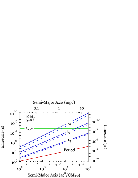
Figure 1.— Different timescales that are relevant to the evolution of orbits of stars in the vicinity of Sgr A^∗, as a function of their semi-major axes. The red line shows the periods of the orbits. The blue lines show the timescales for the precession of the periapsis ($t_{\rm S}$), for the precession of the orbital plane due to frame dragging ($t_{\rm J}$), and for the precession of the orbital frame due to the quadrupole moment of the spacetime ($t_{\rm Q}$); the black-hole spin is taken to be $\chi=0.3$ and solid and dashed lines correspond to eccentricities of 0.5 and 0.8, respectively. The green line ($t_{\rm w,-7}$) shows the characteristic timescale for orbital evolution of a $10M_{\odot}$ star due to the presence of a stellar wind at a mass loss rate of $10^{-7}M_{\odot}$ yr^-1, for $\eta$ set equal to zero.

2.3. Tidal Dissipation of Orbital Energy

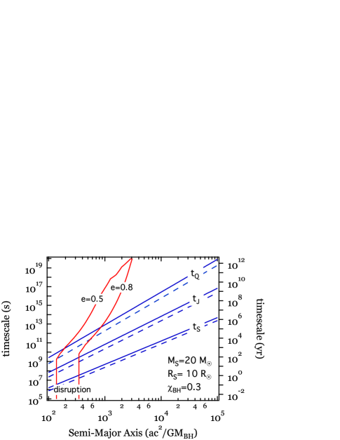
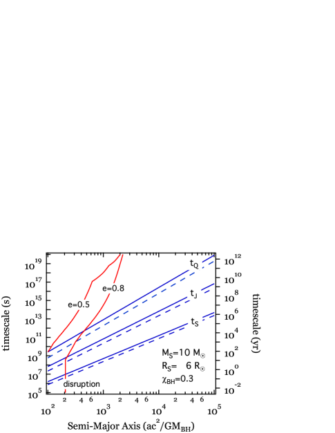
Figure 2.— The blue lines show the dynamical timescales, as in Figure 1. The red lines show the characteristic timescale for orbital evolution due to the tidal dissipation of the orbital energy, for two different values of the eccentricity. The vertical segments of the red lines indicate the semi-major axes at which the stars are tidally disrupted at periastron. The two panels correspond to a 20 $M_{\odot}$ and a 10 $M_{\odot}$ star. In both cases, the black-hole spin is taken to be equal to $\chi=0.3$.

The tidal deformations excited at each periastron passage transfer some of the orbital energy into modes within the volume of the star (see Alexander 2006 for a review of stellar processes around Sgr A^∗). Since the orbital energy loss is proportional to the number of passages (Li & Loeb 2012), we can use the approach of Press & Teukolsky (1977) to estimate the rate of dissipation of orbital energy as

$$\frac{\Delta E}{\Delta t}\simeq\left(\frac{GM_{\rm S}^{2}}{PR_{\rm S}}\right)\left(\frac{M_{\rm BH}}{M_{\rm S}}\right)^{2}\sum_{l=2,3,...}\left(\frac{R_{\rm S}}{R_{\rm p}}\right)^{2l+2}T_{l}(\eta)\;.$$ (10)

Here $R_{\rm p}=a(1-e)$ is the periastron distance, $R_{\rm S}$ is the radius of the star, and $T_{l}(\eta)$ are appropriate dimensionless functions of the quantity

$$\eta\equiv\left(\frac{M_{\rm S}}{M_{\rm S}+M_{\rm BH}}\right)^{1/2}\left(\frac{R_{\rm p}}{R_{\rm S}}\right)^{3/2}$$ (11)

that describe the excitation of modes with different spherical harmonic index $l$.

In detail,

$$T_{l}(\eta)=2\pi^{2}\sum_{n,m}|Q_{nl}|^{2}|K_{nlm}|^{2}\;,$$ (12)

where $n$ is the mode order and $m$ is the other spherical harmonic index. The excited modes have $l>1$ and $-l<m<l$. The coefficient $K_{nlm}$ represents the coupling to the orbit,

$$K_{nlm}=\frac{W_{lm}}{2\pi}\int_{-\infty}^{\infty}dt\left[\frac{R_{p}}{r(t)}\right]^{l+1}\rm{exp}\{i[\omega_{n}t+m{\Phi(t)}]\},$$ (13)

where $r(t)$ is the instantaneous distance between the star and Sgr A^∗, $\omega_{n}$ is the mode frequency, $\Phi(t)$ is the true anomaly, and

$$W_{lm} = (-1)^{(l+m)/2}\left[\frac{4\pi}{(2l+1)}(l-m)!(l+m)!\right]^{1/2}$$ (14)

$$\qquad\left[2^{l}\frac{(l-m)}{2}!\frac{(l+m)}{2}!\right]^{-1}\;.$$

The tidal overlap integral $Q_{nl}$ represents the coupling of the tidal potential to a given mode, i.e.,

$$Q_{nl}=\int_{0}^{1}R^{2}dR\rho(R)lR^{l-1}[\xi_{nl}^{\cal R}+(l+1)\xi_{nl}^{\cal S}]\;,$$ (15)

where $\rho(R)$ is the stellar density profile as a function of radius $R$ and $\xi(R)=[\xi_{nl}^{\cal R}(R)\hat{e}_{R}+\xi_{nl}^{\cal S}(R)R\nabla]Y_{lm}(\theta,\phi)$ is the mode eigenfunction, with $\xi_{nl}^{\cal R}$ and $\xi_{nl}^{\cal S}$ being its radial and poloidal components, respectively. We obtain the appropriate stellar density profile from the MESA code (Paxton et al. 2011) and compute the mode eigenfunctions with the ADIPLS code (Christensen-Dalsgaard 2008).

Because the energy gain in each passage depends on $({R_{S}}/{R_{p}})^{2l+2}$ and the values of $Q_{nl}$ and $K_{nlm}$ are similar for modes with different values of $l$, the quadrupole ($l=2$) modes gain the most energy during the tidal excitation (the $l=0$ and $l=1$ modes are not excited). For this reason, we focus, hereafter, on the $l=2$ modes.

The characteristic timescale for orbital evolution due to tidal dissipation is

$$t_{\rm d} \equiv \frac{E}{\Delta E/\Delta t}$$ (16)

$$= \frac{\pi R_{\rm S}}{c}\left(\frac{GM_{\rm BH}}{c^{2}R_{\rm S}}\right)^{6}\left(\frac{M_{\rm S}}{M_{\rm BH}}\right)\left(\frac{ac^{2}}{GM_{\rm BH}}\right)^{13/2}(1-e)^{6}T_{2}^{-1}$$

$$= 1.37\times 10^{-4}\left(\frac{M_{\rm BH}}{4\times 10^{6}~{}M_{\odot}}\right)^{5}\left(\frac{R_{\rm S}}{10~{}R_{\odot}}\right)^{-5}\left(\frac{M_{\rm S}}{20~{}M_{\odot}}\right)$$

$$\qquad\left(\frac{ac^{2}}{GM_{\rm BH}}\right)^{13/2}\left(1-e\right)^{6}T_{2}^{-1}(\eta)~{}\mbox{s}\;,$$

and is shown in Figure 2 for two main-sequence stars with masses $10M_{\odot}$ and $20M_{\odot}$.

If the star at periastron reaches inside the tidal radius

$$R_{\rm t}=R_{\rm S}\left(\frac{M_{\rm BH}}{M_{\rm S}}\right)^{1/3}\;,$$ (17)

it gets disrupted. For simplicity, we ignore here the fact that, if the periastron distance is smaller than $4-5$ times the tidal radius, the repeated heating of the star at each passage will make it vulnerable to tidal disruption (Li & Loeb 2012). Requiring $R_{\rm p}\geq R_{\rm t}$ sets a lower limit on the semi-major axis of the stellar orbit, i.e.,

$$\left(\frac{ac^{2}}{GM_{\rm BH}}\right) \geq \frac{68.9}{1-e}\left(\frac{R_{\rm S}}{10~{}R_{\odot}}\right)$$ (18)

$$\qquad\left(\frac{M_{\rm BH}}{4\times 10^{6}~{}M_{\odot}}\right)^{-2/3}\left(\frac{M_{\rm S}}{20~{}M_{\odot}}\right)^{-1/3}\;.$$

The tidal limit is shown as the vertical portion of the red lines in Figure 2. At orbital separations larger than this limit, the tidal evolution of the stellar orbits is never fast enough to compete with the precession of the orbital planes due to frame dragging. On the other hand, the orbital plane precession due to the quadrupole moment of the black hole for stars with semi-major axes a few times larger than the tidal limit will be masked by the orbital evolution due to tidal effects.

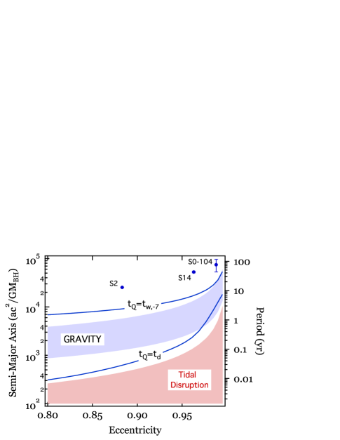
Figure 3.— The two blue curves show the loci of orbital parameters for stars around Sgr A^∗ at which the timescale of orbital-plane precession due to the quadrupole moment of the black hole ($t_{\rm Q}$) is equal to the orbital evolution timescale due to stellar winds ($t_{\rm w,-7}$) or due to tides ($t_{\rm d}$). In order for stars to follow nearly test-particle trajectories, their orbital parameters have to lie between the two curves. The blue shaded area shows the range of orbital parameters for which frame dragging will be detectable with GRAVITY at a signal-to-noise ratio of 5, assuming a range of astrometric accuracies between $10-200~{}\mu$arcsec. The red shaded area show the range of orbital parameters that lead to the tidal disruption of the star at periapsis. All curves are for a black-hole spin of $\chi=0.3$ and a 10 $M_{\odot}$ star. The three filled circles show the orbital parameters of the three stars nearest to Sgr A^∗ that are presently known.

3. DISCUSSION

We explored whether deviations of the orbits of star around Sgr A^∗ from test particle trajectories due to stellar winds and tides may compromise the measurements of relativistic effects. Figure 3 summarizes our results for an illustrative case of a $10~{}M_{\odot}$ star and a black-hole spin of $\chi=0.3$. The two blue curves in this figure show the combinations of semi-major axes and orbital eccentricities for which the timescale of orbital plane precession due to the quadrupole moment of the black hole is equal to the orbital evolution timescale due to the wind-mass loss ($t_{\rm w}=t_{\rm Q}$) and due to tides ($t_{\rm d}=t_{\rm Q}$). In order for a stellar orbit not to be affected significantly by either of the two effects, its parameters need to be in between the two curves.

For comparison, we calculate the signal-to-noise ratio at which the precession of the orbital plane of a star due to frame dragging will be detected, in the near future, using the adaptive-optics assisted interferometer GRAVITY. Following Weinberg et al. (2005), we write the signal-to-noise ratio as

$$S=\frac{8\pi\chi}{a^{1/2}(1+e)^{1/2}(1-e)^{3/2}}\left(\frac{GM_{\rm BH}}{Dc^{2}}\right)^{3/2}\frac{N_{\rm orb}{\cos\psi}}{\delta\theta}\;,$$ (19)

where $D$ is the distance to the black hole, $N_{\rm orb}$ is the number of orbits monitored, $\cos\psi$ is the inclination of the orbit, and $\delta\theta$ is the astrometric accuracy of each measurement. Assuming that we monitor a particular orbit for a time $\Delta T$, we can rewrite this expression as

$$S = \frac{9\times 10^{6}\cos\psi}{(1+e)^{1/2}(1-e)^{3/2}}\left(\frac{\chi}{0.3}\right)\left(\frac{\Delta T}{10~{}\mbox{yr}}\right)\left(\frac{D}{8.4~{}\mbox{kpc}}\right)^{-1}$$ (20)

$$\qquad\qquad\left(\frac{\delta\theta}{10~{}\mu\mbox{arcsec}}\right)^{-1}\left(\frac{ac^{2}}{GM_{\rm BH}}\right)^{-2}\;.$$

The astrometric accuracy of GRAVITY is expected to be $\sim 200~{}\mu$arcsec for a faint star of $m_{\rm K}\simeq 18.8$ and $\sim 10~{}\mu$arcsec for a brighter star of $m_{\rm K}=16.3$. Requiring a signal-to-noise ratio of 5 for this range of astrometric accuracies and for the typical parameters used in the above equation places an upper limit on the semi-major axes of orbits as a function of their eccentricity. This range of upper limits is shown as the blue-shaded region in Figure 3.

For all but the most eccentric orbits for which GRAVITY will be able to detect orbital-plane precession due to frame dragging, both effects of stellar winds and tides do not preclude by themselves the measurement of the quadrupole moment of the black hole. On the other hand, for highly eccentric orbits ($e>0.96$), the tidal dissipation of orbital energy for massive stars occurs at similar timescales as the orbital-plane precession due to the quadrupole moment of the black hole. As a result, it needs to be taken into account as a possible source of systematic uncertainties in measuring the quadrupole moment of the black hole and in testing the no-hair theorem.

References

- Alexander (2006) Alexander, T. 2006, Journal of Physics Conference Series, 54, 243
- Christensen-Dalsgaard (2008) Christensen-Dalsgaard, J., 2008, Ap&SS, 316, 113
- Doeleman et al. (2008) Doeleman, S. S., et al. 2008, Nature, 455, 78
- Eisenhauer et al. (2011) Eisenhauer, F., Perrin, G., Brandner, W., et al. 2011, The Messenger, 143, 16
- Fish et al. (2009) Fish, V. L., & Doeleman, S. S. 2009, arXiv:0906.4040
- Genzel et al. (2010) Genzel, R., Eisenhauer, F., & Gillessen, S. 2010, Reviews of Modern Physics, 82, 3121
- Ghez et al. (2012) Ghez, A. M., Morris, M. R., Do, T., et al. 2012, Twelfth Marcel Grossmann Meeting on General Relativity, 420
- Ghez et al. (2008) Ghez, A. M., et al. 2008, ApJ, 689, 1044
- Gillessen et al. (2009) Gillessen, S., Eisenhauer, F., Trippe, S., Alexander, T., Genzel, R., Martins, F., & Ott, T. 2009, ApJ, 692, 1075
- Johannsen & Psaltis (2010) Johannsen, T., & Psaltis, D. 2010, ApJ, 718, 446
- Li & Loeb (2012) Li, G., & Loeb, A. 2012, 2012, arXiv:1209.1104
- Liu et al. (2012) Liu, K., Wex, N., Kramer, M., Cordes, J. M., & Lazio, T. J. W. 2012, ApJ, 747, 1
- Martins et al. (2008) Martins, F., Gillessen, S., Eisenhauer, F., et al. 2008, ApJ, 672, L119
- Meyer et al. (2012) Meyer, L., Ghez, A. M., Schödel, R., et al. 2012, Science, 338, 84
- Merritt et al. (2010) Merritt, D., Alexander, T., Mikkola, S., & Will, C. M. 2010, Phys. Rev. D, 81, 062002
- Paxton et al. (2011) Paxton, B., Bildsten, L., Dotter, A., et al. 2011, ApJS, 192, 3
- Pfahl & Loeb (2004) Pfahl, E., & Loeb, A. 2004, ApJ, 615, 253
- Press & Teukolsky (1977) Press, W. H., & Teukolsky, S. A. 1977, ApJ, 213, 183
- Psaltis (2012) Psaltis, D. 2012, ApJ, 759, 130
- Sadeghian & Will (2011) Sadeghian, L., & Will, C. M. 2011, Classical and Quantum Gravity, 28, 225029
- Stone et al. (2012) Stone, J. M., Eisner, J. A., Monnier, J. D., et al. 2012, ApJ, 754, 151
- Weinberg et al. (2005) Weinberg, N. N., Milosavljević, M., & Ghez, A. M. 2005, ApJ, 622, 878
- Will (2008) Will, C. M. 2008, ApJ, 674, L25