UT-12-42

IPMU12-0225

Skewness Dependence of GPD / DVCS,
Conformal OPE and AdS/CFT Correspondence I:
— Wavefunction of Regge Trajectory —

Ryoichi Nishio^1,2 and Taizan Watari²

¹Department of Physics, University of Tokyo, Tokyo 113-0033, Japan

²Institute for the Physics and Mathematics of the Universe, University of Tokyo, Kashiwano-ha 5-1-5, 277-8583, Japan

1 Introduction

In this article, we extend AdS/CFT technique to study a class of hadron scattering processes at high energy. Although we cannot expect gravitational “dual” descriptions to be perfectly equivalent to the QCD for high-energy scattering at the quantitative level, yet we still hope to learn, at the qualitative level, non-perturbative information in hadron scattering that is not available in perturbative or lattice QCD calculation [1, 2, 3].

AdS/CFT technique can be used to study not just amplitudes of hadron scattering as a whole, but also to extract information of partons within hadrons [2]. Parton distribution functions are defined by using hadron matrix elements of parton-bilinear operators in QCD, and gravity dual descriptions can be used to determine matrix elements of the gauge singlet operators. The PDF extracted in this way satisfies DGLAP ($q^{2}$-evolution) and BFKL ($\ln(1/x)$-evolution) equations [4]. Thus, the parton information studied in this way may be used to understand non-perturbative issues with partons in a hadron in the real world at qualitative level.

In a series of articles consisting of part I (this one) and part II [5], we study 2-body–2-body scattering between a hadron and a photon (that is possibly virtual) in gravitational dual descriptions; $\gamma^{*}(q_{1})+h(p_{1})\rightarrow\gamma^{(*)}(q_{2})+h(p_{2})$. A special case of this scattering—the forward scattering with $q_{1}=q_{2}$ and $p_{1}=p_{2}$—has been studied extensively in the literature (e.g., [2, 6, 7, 8, 4]) for study of DIS and PDF, and some references also cover the case with $(q_{1}-q_{2})^{2}\neq 0$ (e.g. [8, 4]). This series of articles extend the analysis so that all kinds of skewed cases are covered. In hadron physics, therefore, the kinematics needed for deeply virtual Compton scattering, hard exclusive vector meson production and time-like Compton scattering processes [9] is covered in this analysis. With the full skewness dependence included in this analysis, it is also possible to use the result of this study to bridge a gap between data in such scattering processes at non-zero skewness and the transverse profile of partons in a hadron, which is encoded by the generalized parton distribution functions at zero skewness [10].

For this study, we have to extend the formalism developed in [2, 3] (see also [6, 8, 4]) in a number of points. First, hadron matrix elements of total derivative operators are irrelevant for the $h$–$\gamma^{(*)}$ scattering with zero skewness (like DIS), but they do contribute to the skewed scattering amplitude. This contribution needs to be implemented in the language of gravity dual. Secondly, Pomeron/Reggeon propagators have been treated as if it were for a scalar field in [2, 3, 4], but they correspond to exchange of stringy states with non-zero (arbitrary high) spins; for the study of scattering with non-zero skewness, the polarization of higher spin state propagator should also be treated with care. Finally, this also means that infinitely many gauge degrees of freedom in string theory (which extends the general coordinate transformation of the graviton) need to be dealt with properly.

This article is organized as follows. In this article (part I), we begin in section 2.1 with a review of parametrization of GPD in terms of conformal OPE, because the expansion in a series of conformal primary operators becomes the key concept in using AdS/CFT correspondence (cf [7]). After plainly stating what is need to be done by using gravity dual in section 2.2, we proceed to explain our basic gravity dual setting and idea of how to construct a scattering amplitude of our interest by using string field theory in sections 3 and 4. Section 5 shows the results of computing wavefunctions of spin-$j$ fields on AdS₅, while more detailed account of derivation of the wavefunctions are given in the appendix. Classification of eigenmodes is given in section 5.1, and wavefunctions are presented as analytic functions of the complex spin (angular momentum) variable $j$ in section 5.2 for eigenmodes that turn out to be relevant for the “twist-2” operators in [5]. Those wavefunctions are organized into irreducible representations of conformal algebra in section 5.3; the representation for spin-$j$ primary fields contain more eigenmode components than the those treated by the Pomeron exchange amplitude in the formalism of [3]. These wavefunctions (and propagators) is used in part II [5] in organizing scattering amplitude on AdS₅. Most of the physics results on GPD/DVCS are deferred to [5], and part I (this article) focuses on technical development that may also be of value from perspectives of formal theory.

2 Our Approach: Conformal OPE and Gravity Dual

2.1 Review: Conformal OPE of DVCS Amplitude

Notation and Conventions

Deeply virtual Compton scattering $e+h\rightarrow e+h+\gamma$ (DVCS), hard exclusive vector meson production $e+h\rightarrow e+h+V$ (VMP) and time-like Compton scattering processes $e+h\rightarrow e+h+e^{+}e^{-}$ (TLC) are shown in Figure 1 (a, b), (c) and (d), respectively.

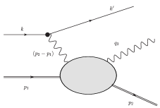
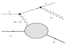
(a) DVCS-Compton	(b) DVCS-BH
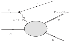
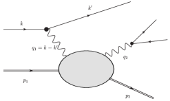
(c) VMP	(d) TCS

Figure 1: (a, b) are diagrams contributing to the deeply virtual Compton scattering process, (c) is the exclusive vector meson production process, and finally (d) is the time-like Compton scattering process.

As a part of all these processes, the photon–hadron 2-body to 2-body scattering amplitude

$${\cal M}(\gamma^{\ast}h\rightarrow\gamma^{(\ast)}h)=(\epsilon_{1}^{\mu})T_{\mu\nu}(\epsilon_{2}^{\nu})^{\ast}.$$ (1)

is involved. This 2-body to 2-body scattering with this exclusive choice of the final states (2) is truly non-perturbative information, and this is the subject of this article. Because the “final state” photon is required to be on-shell $q_{2}^{2}=0$ in DVCS and time-like $q_{2}^{2}<0$ in VMP and TLC, we are interested in developing a theoretical framework to calculate this non-perturbative amplitude in the case $q_{2}^{2}$ is different from space-like $q_{1}^{2}>0$.

Just like in QCD / hadron literature, we used the following notation for Lorentz invariant kinematical variables:

$$p^{\mu} =\frac{1}{2}(p_{1}^{\mu}+p_{2}^{\mu}), q^{\mu} =\frac{1}{2}(q_{1}^{\mu}+q_{2}^{\mu}), \Delta^{\mu} =p_{2}^{\mu}-p_{1}^{\mu}=q_{1}^{\mu}-q_{2}^{\mu},$$ (2)

$$x =\frac{-q^{2}}{2p\cdot q}, \eta =\frac{-\Delta\cdot q}{2p\cdot q}, s =W^{2}=-(p+q)^{2}, t =-\Delta^{2}.$$ (3)

$\eta$ is called skewness; in the scattering process of our interest, $q_{1}^{2}=q^{2}+\Delta^{2}/4+q\cdot\Delta$ and $q_{2}^{2}=q^{2}+\Delta^{2}/4-q\cdot\Delta$ are not the same, and hence the skewness does not vanish. We will focus on high-energy scattering; for typical energy scale of hadron masses / confinement scale $\Lambda$, we assume that

$$\Lambda^{2}\ll q_{1}^{2},\;\;W^{2},\quad{\rm while}\quad|t|\lesssim{\cal O}(\Lambda).$$ (4)

The photon–hadron scattering amplitude (Figure 2) in the real-world QCD (where all charged partons are fermions), the Compton tensor is given by the hadron matrix element with insertion of two QED currents $J^{\mu}$,

$$T^{\mu\nu}=i\int d^{4}xe^{-iqx}\langle{h(p_{2})}|T\{J^{\nu}(x/2)J^{\mu}(-x/2)\}|{h(p_{1})}\rangle.$$ (5)

For simplicity, we assume that the target hadron is a scalar, and further pay attention only to the structure function $V_{1}$ appearing in the gauge-invariant decomposition of the Compton tensor:

$$T^{\mu\nu}= V_{1}P[q_{1}]^{\mu\rho}P[q_{2}]^{\nu}_{\rho}+V_{2}(p\cdot P[q_{1}])^{\mu}(p\cdot P[q_{2}])^{\nu}+V_{3}(q_{2}\cdot P[q_{1}])^{\mu}(q_{1}\cdot P[q_{2}])^{\nu}$$

$$+V_{4}(p\cdot P[q_{1}])^{\mu}(q_{1}\cdot P[q_{2}])^{\nu}+V_{5}(q_{2}\cdot P[q_{1}])^{\mu}(p\cdot P[q_{2}])^{\nu}+A\epsilon^{\mu\nu\rho\sigma}q_{1\rho}q_{2\sigma}.$$ (7)

Those structure functions, $V_{1,2,3,4,5}(x,\eta,t,q^{2})$, should be expressed in terms of the kinematical variables $x,\eta$ and $t$, and our primary purpose of this article is to study how the structure functions depend on the skewness $\eta$.

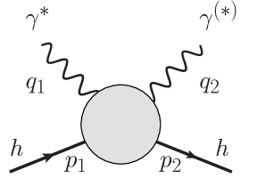
Figure 2: photon–hadron 2-body to 2-body scattering amplitude

Light-cone Operator Product Expansion

The light-cone operator product expansion (OPE) can be applied to the product of currents $T\left\{J^{\nu}J^{\mu}\right\}$, before evaluating it as a hadron matrix element. Let the expansion be

$$i\int d^{4}xe^{-iqx}T\{J^{\nu}(x/2)J^{\mu}(-x/2)\}=\sum_{I}{\cal C}_{I\>\rho_{1}\dots\rho_{j_{I}}}^{\mu\nu}(q){\cal O}_{I}^{\rho_{1}\dots\rho_{j_{I}}}(0;q^{2})$$ (8)

for some basis of local operators ${\cal O}_{I}^{\rho_{1}\cdots\rho_{j_{I}}}$ renormalized at $\mu^{2}=q^{2}$. $C^{\mu\nu}_{I\;\rho_{1}\cdots\rho_{j_{I}}}$ is the corresponding Wilson coefficients renormalized at $\mu^{2}=q^{2}$. If we were to evaluate these local operators on the right-hand side with the same states as bra and ket, $\langle{h(p_{2})}|$ and $|{h(p_{1})}\rangle$ with $p_{2}^{\mu}=p_{1}^{\mu}$, then the Compton tensor and its structure functions do not receive non-zero contributions from local operators that are given by total derivative of some other local operators. In the case of our interest, however, such operators do contribute.

Let us take a series of operators in QCD that are called twist-2 operators in the weak coupling limit. The twist-2 operators in the flavor non-singlet sector are labeled by two integers, $j,l$,

$${\cal O}^{\alpha}_{j,l}:=\left[(-i)^{j+l}\partial^{\mu_{j+1}}\cdots\partial^{\mu_{j+l}}\bar{\Psi}_{a}\gamma^{\mu_{1}}\left(\overleftrightarrow{D}\right)^{\mu_{2}}\cdots\left(\overleftrightarrow{D}\right)^{\mu_{j}}\;\lambda^{\alpha}_{ab}\Psi_{b}\right]_{{\rm t.s.t.l.}}(0;q^{2}),$$ (9)

with a $N_{F}\times N_{F}$ flavor matrix $(\lambda^{\alpha})_{ab}$. Similarly there are two series of twist-2 operators with the label $j,l$, given by quark bilinear and gluon bilinear. Here, these operators are made totally symmetric and traceless (t.s.t.l) in the $j+l$ Lorentz indices in order to make it transform in an irreducible representation of the Lorentz group $\mathop{\rm SO}(3,1)$. $\overleftrightarrow{D}:=\overrightarrow{D}-\overleftarrow{D}$.

Suppose that the hadron matrix element of the operator ${\cal O}^{\alpha}_{j,l}$ is given by

$$\langle{h(p_{2})}|{\cal O}^{\alpha}_{j,l}|{h(p_{1})}\rangle=\sum_{k=0}^{j}\left[\Delta^{\mu_{1}}\cdots\Delta^{\mu_{k+l}}p^{\mu_{k+l+1}}\cdots p^{\mu_{j+l}}\right]_{{\rm t.s.t.l.}}A_{j,k}(t;q^{2})(-2)^{j-k};$$ (10)

the reduced matrix element $A^{\alpha}_{j,k}(t)$ is non-perturbative information and cannot be determined by perturbative QCD. If we pay attention only to Wilson coefficients $C^{\mu\nu}_{j,l,\alpha;\mu_{1}\cdots\mu_{j+l}}$ that are proportional to $\eta^{\mu\nu}$, and denote them by

$$\eta^{\mu\nu}{\cal C}^{\alpha}_{j,l}\frac{q_{\rho_{1}}\cdots q_{\rho_{j+l}}}{(q^{2})^{j+l}},$$ (11)

then the twist-2 flavor non-singlet contribution to the structure function $V_{1}$ becomes

$$V_{1}\simeq\sum_{j,l}{\cal C}^{\alpha}_{j,l}\frac{1}{x^{j+l}}\sum_{k=1}^{j}A^{\alpha}_{j,k}(t;q^{2})\eta^{k+l}=:\sum_{j}{\cal C}^{\alpha}_{j}\left(\frac{\eta}{x}\right)\frac{1}{x^{j}}A^{\alpha}_{j}(\eta,t;q^{2}),$$ (12)

where ${\cal C}^{\alpha}_{j}(\eta/x):=\sum_{l=0}^{\infty}{\cal C}^{\alpha}_{j,l}(\eta/x)^{l}$, and $A^{\alpha}_{j}(\eta,t):=\sum_{k=0}^{j}\eta^{k}A^{\alpha}_{j,k}(t)$. If the structure function $V_{1}$ receives only from even $j\in\mathbb{Z}$, then this $j$-summation is rewritten as

$$V_{1}(x,\eta,t;q^{2})\simeq-\int\frac{dj}{4i}\frac{1+e^{-\pi ij}}{\sin(\pi j)}{\cal C}^{\alpha}_{j}\left(\frac{\eta}{x}\right)\frac{1}{x^{j}}A^{\alpha}_{j}(\eta,t;q^{2})$$ (13)

in the form of inverse Mellin transformation; here, ${\cal C}^{\alpha}_{j}(\eta,x)$ and $A^{\alpha}_{j}(\eta,t;q^{2})$ are now meant to be holomorphic functions on $j$ (possibly with some poles and cuts) that coincide with the original ones at $j\in 2\mathbb{Z}$. Precisely the same story holds also for flavor-singlet sector.

Because the structure function is given by the inverse Mellin transform of a product of the signature factor $[1+e^{-\pi ij}]/\sin(\pi j)$, Wilson coefficients ${\cal C}^{\alpha}_{j}$ and hadron matrix elements $A^{\alpha}_{j}$, it can be regarded as a convolution of inverse Mellin transforms of those three factors. The inverse Mellin transform of the signature factor becomes

$$\int\frac{dj}{2\pi i}\frac{1}{x^{j}}\frac{\pi}{2}\frac{\mp[1\pm e^{-\pi ij}]}{\sin(\pi j)}=\frac{-1}{2}\left[\frac{1}{1-x+i\epsilon}\pm\frac{1}{1+x}\right],$$ (14)

which corresponds to propagation of the parton in perturbative calculation [11], and the inverse Mellin transform of the matrix element is defined as the generalized parton distribution:

$$H^{\alpha}(x,\eta,t;\mu^{2}=q^{2})=\int\frac{dj}{2\pi i}\frac{1}{x^{j}}A_{j}(\eta,t;\mu^{2}=q^{2}).$$ (15)

Generalized parton distribution (GPD) $H^{\alpha}(x,\eta,t;\mu^{2})$ of a hadron $h$ is a non-perturbative information, just like the ordinary PDF, which is obtained by simply setting $\eta=0$ and $t=0$. For phenomenological fit of experimental data of DVCS and VMP, some function form of the GPD needs to be assumed, because of the convolution involved in the scattering amplitude. Setting up a model (and assuming a function form) for the non-perturbative information in terms of $A_{j}(\eta,t;q^{2})$ rather than the GPD itself $H(x,\eta,t;q^{2})$ is called dual parametrization [12], and some phenomenological ansätze have been proposed. In this article, we aim at deriving qualitative form of $A_{j}(\eta,t)$ by using gravitational dual (that is analytic in $j$), instead of assuming the form of $A_{j}(\eta,t)$.

Renormalization and OPE in dilatation eigenbasis

Remembering that the distinction between the $\gamma^{*}+h\rightarrow\gamma+h$ scattering amplitude and GPD originates from the factorization into the Wilson coefficients and local operators (and their matrix elements), one will notice that the GPD defined in this way should depend on the choice of the basis of local operators. Although the choice of operators ${\cal O}^{\alpha}_{j,l}$ with $j\geq 1$ and $l\geq 0$ in (9) appears to be the most natural (and intuitive) one for the twist-2 operators in the flavor non-singlet sector, there is nothing wrong to take a different linear combinations of these operators as a basis, when the corresponding Wilson coefficients also become linear combinations of what they are for ${\cal O}^{\alpha}_{j,l}$. Given the fact that the operators ${\cal O}^{\alpha}_{j,l}$ mix with one another under renormalization, it is not compulsory for us to stick to the basis ${\cal O}^{\alpha}_{j,l}$.

Under the perturbation of QCD, the flavor non-singlet twist-2 operators are renormalized under

$$\mu\frac{\partial}{\partial\mu}\>[{\cal O}_{j-m,m}(0;\mu^{2})]=-[\gamma^{(j)}]_{mm^{\prime}}\>[{\cal O}_{j-m^{\prime},m^{\prime}}(0;\mu^{2})];$$ (16)

because operators can mix only with those with the same number of Lorentz indices, the anomalous dimension matrix is block diagonal in the basis of ${\cal O}^{\alpha}_{j,l}$. The $j\times j$ matrix for the operators ${\cal O}^{\alpha}_{j-m,m}$ ($m=0,\cdots,j-1$) is denoted by $[\gamma^{(j)}]$. This matrix is upper triangular in this basis, and the diagonal entries are given by the anomalous dimensions of the twist-2 spin-$j$ operators without a total derivative:

$$\left[\gamma^{(j)}\right]_{mm}=\gamma(j-m).$$ (17)

Therefore, the eigenvalues of the anomalous dimension matrix is $\left\{\gamma(j-m)\right\}_{m=0,\cdots,j-1}$ in this diagonal block, and the corresponding operator $\overline{{\cal O}}^{\alpha}_{j-m-1,m}$ is a linear combination of operators ${\cal O}_{j-m^{\prime},m^{\prime}}$ with $m^{\prime}=m,\cdots,j-1$ [13]. The corresponding Wilson coefficient $\overline{C}^{\alpha}_{j-m-1,m}$ for such an operator is a linear combination of ${\cal C}^{\alpha}_{j-m^{\prime},m^{\prime}}$ with $m^{\prime}=m,\cdots,0$. In this operator basis, matrix elements and Wilson coefficients renormalize multiplicatively, without mixing.

In this new basis of local operator, the structure function becomes

$$V_{1}\simeq\sum_{n,K}\overline{\cal C}^{\alpha}_{n,K}\frac{1}{x^{n+1+K}}\sum_{k}\overline{A}^{\alpha}_{n+1,k}(t;\mu^{2})\eta^{K+k}=:\sum_{n}\overline{C}^{\alpha}_{n}\left(\frac{\eta}{x}\right)\frac{1}{x^{n+1}}\overline{A}^{\alpha}_{n+1}(\eta,t;\mu^{2}),$$ (18)

where

$$\overline{C}^{\alpha}_{n}=\sum_{K=0}^{\infty}\overline{C}^{\alpha}_{n,K}\left(\frac{\eta}{x}\right)^{K},$$ (19)

and $\overline{A}^{\alpha}_{n+1,k}(t;\mu^{2})$ is the reduced matrix element of the operator $\overline{\cal O}^{\alpha}_{n,0}(0;\mu^{2})$. The structure function is therefore written as yet another inverse Mellin transform

$$V_{1}\simeq-\int\frac{dj}{4i}\frac{1+e^{-\pi i}}{\sin(\pi j)}\overline{C}^{\alpha}_{j-1}(\eta/x)\frac{1}{x^{j}}\overline{A}^{\alpha}_{j}(\eta,t;\mu^{2}).$$ (20)

Yet another GPD can also be defined by using $\overline{A}^{\alpha}$, instead of $A^{\alpha}_{j}(\eta,t;q^{2})$.

$$\overline{H}(x,\eta,t;\mu^{2})=\int\frac{dj}{2\pi i}\frac{1}{x^{j}}\overline{A}^{\alpha}_{j}(\eta,t;\mu^{2}).$$ (21)

When it comes to the description of the $\gamma^{*}+h\rightarrow\gamma+h$ scattering amplitude as a whole, it does not matter which operator basis is used. Although we need GPD rather than the scattering amplitude in order to talk about the distribution of partons in the transverse directions in a hadron, yet we only need GPD at $\eta=0$. Thus, the newly defined GPD $\overline{H}$ does just as good a job as $H$ defined in (15); they are the same at $\eta=0$.

Even within the dual parametrization approach, it has been advantageous to use this operator basis, because it becomes much easier to implement a phenomenological assumption (function form) of $\overline{A}^{\alpha}_{j}(\eta,,t;\mu^{2})$ that is consistent with renormalization group flow [9].

Conformal OPE

Although the hadron matrix element is essentially non-perturbative, and is not calculable within perturbative QCD, more discussion has been made on the Wilson coefficients $\overline{C}^{\alpha}_{n,K}$. They still have to be calculated order by order in perturbation theory, if one is interested strictly in the QCD of the real world. If one is interested in gauge theories that are more or less “similar” to QCD, however, stronger statements can be made for a system with higher symmetry: conformal symmetry. One can think of ${\cal N}=4$ super Yang–Mills theory or ${\cal N}=1$ supersymmetric $\mathop{\rm SU}(N)\times\mathop{\rm SU}(N)$ gauge theory of [15] as an example of theories with exact (super) conformal symmetry. The QED probe in the real world QCD can be replaced by gauging global symmetries (such as (a part of) $\mathop{\rm SU}(4)$ R-symmetry of ${\cal N}=4$ super Yang–Mills theory and $\mathop{\rm SU}(2)\times\mathop{\rm SU}(2)\times\mathop{\rm U}(1)$ symmetry of [15]). By applying the conformal symmetry, one can derive stronger statements on the Wilson coefficients appearing in OPE of primary operators (like conserved currents).

Suppose that we are interested in the OPE of two primary operators, $A$ and $B$, that are both scalar under $\mathop{\rm SO}(3,1)$. If we take the basis of local operators for the expansion to be primary operators $\overline{\cal O}_{n}$ (with $j_{n}$ Lorentz indices and $l_{n}$ scaling dimension) and their descendants $\partial^{K}\overline{\cal O}_{n}$ (with $j_{n}+K$ Lorentz indices),

$$T\left\{A(x)B(0)\right\}=\sum_{n}\left(\frac{1}{x^{2}}\right)^{\frac{1}{2}(l_{A}+l_{B}-l_{n}+j_{n})}\sum_{K=0}^{\infty}c_{n,K}\frac{x^{\rho_{1}}\cdots x^{\rho_{j_{n}+K}}}{(x^{2})^{j_{n}+K}}[\partial^{K}\overline{\cal O}_{n}(0)]_{\rho_{1}\cdots\rho_{j_{n}+K}},$$ (22)

then the conformal symmetry determines all the coefficients of the descendants $c_{n,K}$ ($K\geq 1$) in terms of that of the primary operator, $c_{n,0}=:c_{n}$. Ignoring the mixture of non-traceless contributions, one finds that [16]

$$T\left\{A(x)B(0)\right\}\simeq\sum_{n}\left(\frac{1}{x^{2}}\right)^{\frac{1}{2}(l_{A}+l_{B}-l_{n}+j_{n})}\!\!\!\!\!\!\!\!\!\!\!\!\!\!\!\!\!\!\!\!\!\!\!\!\!\!\!x^{\rho_{1}}\cdots x^{\rho_{j_{n}}}c_{n}{}_{1}F_{1}((l_{A}-l_{B}+l_{n}+j_{n})/2,l_{n}+j_{n};x\cdot\partial)[\overline{\cal O}_{n}(0)]_{\rho_{1}\cdots\rho_{j_{n}}}.$$ (23)

Questions of real interest to us is the OPE conserved currents $J^{\nu}$ and $J^{\mu}$. They are not scalars of $\mathop{\rm SO}(3,1)$, but the same logic as in [16] can be used also to show that, in the terms with Wilson coefficients proportional to $\eta^{\mu\nu}$,

$$T\left\{J^{\nu}(x)J^{\mu}(0)\right\}\simeq\eta^{\mu\nu}\sum_{n}\left(\frac{1}{x^{2}}\right)^{3-\frac{\tau_{n}}{2}}\!\!\!\!\!\!\!\!\!\!\!x^{\rho_{1}}\cdots x^{\rho_{j_{n}}}c_{n}{}_{1}F_{1}((l_{n}+j_{n})/2,l_{n}+j_{n};x\cdot\partial)[\overline{\cal O}_{n}(0)]_{\rho_{1}\cdots\rho_{j_{n}}}+\cdots,$$ (24)

where $\tau_{n}:=l_{n}-j_{n}$ is the twist, mixture of the non-traceless (and hence higher twist) contributions are ignored, and terms with Wilson coefficients without $\eta^{\mu\nu}$ are all omitted here. The scaling dimension of conserved currents $l_{A}=l_{B}=3$ have been used. The momentum space version of the OPE is [17]

$$i\int d^{4}x\;e^{-iq_{2}\cdot x}\;T\left\{J^{\nu}(x)J^{\mu}(0)\right\} \simeq \eta^{\mu\nu}\sum_{n}\frac{(2\pi)^{2}\Gamma\left(\frac{l_{n}+j_{n}-2}{2}\right)}{4^{2-\frac{\tau_{n}}{2}}\Gamma\left(3-\frac{\tau_{n}}{2}\right)}c_{n}\;\frac{(-2i)^{j_{n}}q_{2}^{\rho_{1}}\cdots q_{2}^{\rho_{j_{n}}}}{(q^{2}_{2})^{\frac{\tau_{n}}{2}-1}(q^{2}_{2})^{j_{n}}}$$ (25)

$$\!\!\!\!\!\!\!\!\!\!\!\!\!\!\!\!\!\!\!\!\!\!\!\!\!\!{}_{2}F_{1}\left(\frac{l_{n}+j_{n}}{2},\frac{l_{n}+j_{n}}{2}-1,l_{n}+j_{n};\frac{-2iq_{2}\cdot\partial}{q_{2}^{2}}\right)\overline{\cal O}_{n}(0)+\cdots,$$

or equivalently [19],

$$i\int d^{4}(x-y)e^{-iq\cdot(x-y)}\;T\left\{J^{\nu}(x)J^{\mu}(y)\right\} \simeq \eta^{\mu\nu}\sum_{n}\frac{(2\pi)^{2}\Gamma\left(\frac{l_{n}+j_{n}-2}{2}\right)}{4^{2-\frac{\tau_{n}}{2}}\Gamma\left(3-\frac{\tau_{n}}{2}\right)}c_{n}\;\frac{(-2i)^{j_{n}}q^{\rho_{1}}\cdots q^{\rho_{j_{n}}}}{(q^{2})^{\frac{\tau_{n}}{2}-1}(q^{2})^{j_{n}}}$$ (26)

$$\!\!\!\!\!\!\!\!\!\!\!\!\!\!\!\!\!\!\!\!\!\!\!\!\!\!\!\!\!\!\!\!\!\!\!\!\!\!\!\!\!\!\!\!\!\!\!\!\!\!\!\!\!\!\!\!\!\!\!\!\!\!\!{}_{2}F_{1}\left(\frac{l_{n}+j_{n}-2}{4},\frac{l_{n}+j_{n}}{4},\frac{l_{n}+j_{n}}{2};\left(\frac{iq\cdot\partial}{q^{2}}\right)^{2}\right)\overline{\cal O}_{n}\left(\frac{x+y}{2}\right)+\cdots.$$

Either in the form of (25) or (26), the primary operators $\overline{\cal O}_{n}$ and corresponding coefficients $c_{n}$ are renormalized multiplicatively.

2.2 AdS/CFT Approach

In AdS/CFT correspondence, Type IIB string theory on AdS${}_{5}\times W$ with a 5-dimensional Einstein manifold $W$ would correspond to a gauge theory on $\mathbb{R}^{3,1}$ with an exact conformal symmetry, which is qualitatively different from the QCD in the real world. But the Type IIB string on a geometry that is close to AdS${}_{5}\times W$, but with confining end in the infrared, may be used to extract qualitative lesson on strongly coupled gauge theories with confinement.

In a dual pair of a CFT and a string theory on a background AdS${}_{5}\times W$, primary operators of the CFT are in one to one correspondence with string states on AdS${}_{5}\times W$, and their correlation functions can be calculated by using the wavefunctions of the string states on AdS₅. When the background geometry is changed from AdS${}_{5}\times W$ to some warped geometry that is nearly AdS₅ with an end in the infrared, then the wavefunctions might be used to calculate matrix elements of the corresponding “primary” operators in an almost conformal theory. The correspondence between the operator and string states can be made precise, because they are both classified in terms of representation of the conformal algebra, which is shared by both of the dual theories.

In order to determine GPD $\overline{H}$ in gravitational dual descriptions, it is therefore sufficient to determined wavefunctions of string states corresponding to the “primary” operators of interest. Although there are plenty of literature discussing the correspondence between the (superconformal) primary operators and string states at the supergravity level, it is known that the flavor-singlet twist-2 operators (labeled by the spin $j$) correspond to the stringy excitations with arbitrary high spin $j$ that are in the same trajectory as graviton [20, 3]. Our task is therefore to determine the wavefunctions of such string states. Needless to say, one has to fix all the gauge degrees of freedom associated with string component fields (not just the general coordinate invariance associated with the graviton) before working out the mode decomposition. Furthermore, wavefunctions need to be grouped together properly so that they form an irreducible representation of the conformal group, in order to establish correspondence with a primary operator of the gauge theory side, which also forms an irreducible representation of the conformal group along with its descendants.

It will be clear by the end of this article that all of such technical works is necessary and essential for the purpose of extracting skewness dependence of GPD.

The DVCS $\gamma^{*}+h\rightarrow\gamma^{(*)}+h$ amplitude can be calculated in gravitational dual descriptions in two different ways. One is to use the matrix elements of spin-$j$ primary operators calculated in gravitation dual (as we discussed just above) and combine them with the Wilson coefficients which are governed by the conformal symmetry (see (26)). The other is to calculate disc/sphere amplitude directly, with the vertex operators given (approximately) by using the wavefunctions associated with the target hadron (see sections 3 and 4); in this approach, contributions from operators with higher twists are also included. In this article, we adopt the latter approach. In the resulting expression for the $\gamma^{(*)}+h\rightarrow\gamma+h$ scattering amplitude in gravity dual, however, we can easily identify the structure of conformal OPE (as we will see in [5]), so that we can identify the contributions from the “twist-2” operators.

3 Gravity Dual Settings

A number of warped solutions to the Type IIB string theory has been constructed, and they are believed to be dual to some strongly coupled gauge theories. When the geometry is close to AdS${}_{5}\times W$ with some 5-dimensional Einstein manifold $W$, with weak running of the AdS radius along the holographic radius, the corresponding gauge theory will also have approximate conformal symmetry, and the gauge coupling constant runs slowly. If the “AdS${}_{5}\times W$” geometry has a smooth end at the infra red as in [21], then the dual gauge theory will end up with confinement. Gravitational backgrounds in the Type IIB string theory with the properties we stated above all provide a decent framework of studying qualitative aspects of non-perturbative information associated with gluons/Yang–Mills theory on 3+1 dimensions.

In studying the $h+\gamma^{*}\rightarrow h+\gamma$ scattering process in gravitational dual, we need a global symmetry to be gauged weakly, just like QED for QCD. In Type IIB D-brane constructions of gauge theories that have gravity dual, U(1) subgroups of an R-symmetry or a flavor symmetry on D7-branes can be used as the models of the electromagnetic U(1) symmetry. Therefore, we have in mind gravity dual models on a background that is approximately “AdS${}_{5}\times W$” with a non-trivial isometry group on $W$, or with a D7-brane configuration on it.

Our motivation, however, is not so much in writing down an exact mathematical expression based on a particular gravity dual model that is equivalent to a particular strongly coupled gauge theory, but more in extracting qualitative information of partons in hadrons of confining gauge theories in general. It is therefore more suitable for this purpose to use a simplified set-up that carries common (and essential) features of the Type IIB models that we described above. Throughout this article, we assume pure AdS${}_{5}\times W$ metric background,

$$ds^{2}=G_{MN}dx^{M}dx^{N} =g_{mn}dx^{m}dx^{n}+R^{2}(g_{W})_{ab}d\theta^{a}d\theta^{b},$$ (27)

$$g_{mn}dx^{m}dx^{n} =e^{2A(z)}(\eta_{\mu\nu}dx^{\mu}dx^{\nu}+dz^{2}),\;\;\;e^{2A(z)}=\frac{R^{2}}{z^{2}}.\;\;\;$$ (28)

that is, we ignore the running effect, and we do not specify the 5-dimensional manifold $W$. The dilaton vev is simply assumed to be constant, $e^{\phi}=g_{s}$. Confining effect—the infra-red end of this geometry—can be introduced, for example, by sharply cutting of the AdS₅ space at $z=\Lambda^{-1}$ (hard wall models), or by similar alternatives (soft wall models). We are not committed to a particular implementation of the infra-red cut-off in this article, except in a couple of places where we write down some concrete expressions for illuminating purposes. The energy scale $\Lambda$ associated with (any form of implementation of) the infra-red cut-off corresponds to the confining energy scale in the dual gauge theories. When we consider (simplified version of the) models with D7-branes for flavor, we assume that the D7-brane worldvolume wraps on a 3-cycle on $W$, and extends all the way down to the infra-red end of the holographic radius $z$; i.e., all of $0\leq z\leq\Lambda^{-1}$. This corresponds to assuming massless quarks. In this article, we will not pay attention to physics where spontaneous chiral symmetry breaking is essential.

As we stated earlier, we would like to work out the $h+\gamma^{*}\rightarrow h+\gamma$ scattering amplitude by using the gravity dual models. This is done by summing up sphere / disc amplitudes, along with those with higher genus worldsheets. We will restrict our attention to kinematical regions where saturation is not important (i.e., large $q^{2}$ and/or not too small $x$, and large $N_{c}$). That allows us to focus only on sphere / disc amplitudes, with insertion of four vertex operators corresponding to the incoming and outgoing hadron $h$ and (possibly virtual) photon $\gamma$.

As a string-based model of the target hadron $h$ (that is $\mathop{\rm SO}(3,1)$ scalar), we have in mind either a scalar “glueball” that has non-trivial R-charge, or a scalar meson made of matter fields. The former corresponds to a vertex operator (in the $(-1,-1)$ picture)

$$V(p)=:e^{ip_{\mu}\cdot X^{\hat{\mu}}}\psi^{m}\tilde{\psi}^{n}g_{mn}\Phi(Z;m_{n})Y(\Theta):,$$ (29)

where $Y(\Theta)$ is a “spherical harmonics” on $W$, and the latter to

$$V(p)=:e^{ip_{\mu}\cdot X^{\hat{\mu}}}\psi\Phi(Z;m_{n}):,$$ (30)

where $\psi$ corresponds to the D7-brane fluctuations in the transverse direction. $\Phi(Z)$ is the wavefunction on AdS₅, with the argument promoted to the field on the world sheet. Vertex operators above are approximate expressions in the $(\alpha^{\prime}/R^{2})\sim 1/\sqrt{\lambda}$ expansion in a theory formulated with a non-linear sigma model given by (27). If we are to employ the hard-wall implementation of the infra-red boundary, with the AdS₅ metric without modification, then the wavefunction $\Phi(Z;m_{n})$ is of the form

$$\sqrt{c_{\phi}}\Phi(z;m_{n})=\left(\frac{2\kappa_{5}^{2}}{R^{3}}\right)^{1/2}\sqrt{2}\Lambda z^{2}\frac{J_{\Delta-2}(j_{{\Delta-2},n}\Lambda z)}{J_{\Delta-2}(j_{{\Delta-2},n})}.$$ (31)

The “photon” current in the correlation function/matrix element $T^{\nu\mu}$ in the gauge theory description corresponds to insertion of vertex operators associated with non-renormalizable wavefunctions, rather than to the normalizable wavefunctions (31) for the target hadron state. If we are to employ an R-symmetry current as the string-based model of the QED current, then the corresponding closed string vertex operator is

$$V(q)=:e^{iq_{\mu}\cdot X^{\hat{\mu}}}v_{a}(\Theta)A_{m}(Z;q)(\psi^{a}\tilde{\psi}^{m}+\psi^{m}\tilde{\psi}^{a}):,$$ (32)

with some Killing vector $v_{a}\partial/\partial\theta^{a}$ on $W$. The vertex operator in the case of D7-brane U(1) current is

$$V(q)=:e^{iq_{\mu}\cdot X^{\hat{\mu}}}A_{m}(Z;q)\psi^{m}:.$$ (33)

The wavefunction $A_{m}(Z;q)$ on AdS₅ is of the form

$$A_{\mu}(z;q)= \left[\delta_{\mu}^{\;\hat{\kappa}}-\frac{q_{\mu}q^{\hat{\kappa}}}{q^{2}}\right]\epsilon_{\kappa}(q)(qz)K_{1}(qz)+ q_{\mu}\frac{q^{\hat{\kappa}}\epsilon_{\kappa}(q)}{2q^{2}}(qz)^{2}K_{2}(qz),$$ (34)

$$A_{z}(z;q)= \!\!\!-i\partial_{z}\frac{q^{\hat{\kappa}}\epsilon_{\kappa}(q)}{2q^{2}}(qz)^{2}K_{2}(qz).$$ (35)

Rationale for our choice of the terms proportional to $(q\cdot\epsilon)$ will be explained later on A.4, but those terms should not be relevant in the final result, because of the gauge invariance of $T^{\nu\mu}$. When the infra-red boundary is implemented by the hard wall, $K_{1}(qz)$ should be replaced by $K_{1}(qz)+[K_{0}(q/\Lambda)/I_{0}(q/\Lambda)]I_{1}(qz)$; and $K_{2}(qz)$ by arbitrary linear combination of $K_{2}(qz)$ and $I_{2}(qz)$.

It is not as easy to calculate the sphere/disc amplitudes in practice, however. It has been considered that the parton contributions to $\gamma^{*}+h\rightarrow\gamma^{(*)}+h$ scattering is given by amplitude with states in the leading trajectory with arbitrary high spin being exchanged [3]. Those fields are not scalar on AdS₅ but come with multiple degree of freedom associated with polarizations. As we will see clearly in [5], such polarization of higher spin fields propagating on AdS₅ needs to be treated properly—including such issues as covariant derivatives and kinetic mixing among different polarizations—in gravity dual descriptions, in order to be able to discuss skewness dependence of GPD / DVCS amplitude. Direct impact of the curved background geometry can be implemented through the non-linear sigma model on the world sheet, but one has to define the vertex operators as a composite operator properly in such an interacting theory. Ramond–Ramond background is an essential ingredient in making the warped background metric stable, yet non-zero Ramond–Ramond background cannot be implemented in the NSR formalism.

Instead of world-sheet calculation in the NSR formalism in implementing the effect of curved background (27), we use string field theory action on flat space in this article, and make it covariant. Because the gravity dual set-up of our interest is in the Type IIB string theory, we are thus supposed to use superstring field theory for closed string and open string. In order to avoid technical complications associated with the interacting superstring field theories, however, we employ a sort of toy-model approach by using the cubic string field theory for bosonic string theory.

In our toy-mode approach, we deal with the cubic string field theory on AdS₅ ($\times$ some internal compact manifold), and ignore instability of the background geometry. The probe photon in this toy-model gravity dual set-up will be the massless vector state of the bosonic string theory with the wavefunction (35). The target hadron can be any scalar states, say, the tachyon, with the wavefunction (31). We are to construct a toy-model amplitude of the $h+\gamma^{(*)}\rightarrow h+\gamma^{(*)}$ scattering, by using the 2-to-2 scattering of the massless photon and some scalar in the bosonic string on the AdS₅ background. Clearly one of the cost of this approach (without technical complexity of interacting superstring field theory) is that we have to restrict our attention to the Reggeon exchange (flavor non-singlet) amplitude. The amplitude constructed in this way is certainly not faithful to the equations of the Type IIB string theory, either. Since our motivation is not in constructing yet another exact solution to superstring theory, however, we still expect that this (flavor non-singlet) toy-mode amplitude in bosonic string still maintains some fragrance of hadron scattering amplitude to be calculated in superstring theory.

4 Cubic String Field Theory

Section 4.1 summarizes technical details of cubic string field theory that we need in later sections and in part II [5]. We then move on in section 4.2 to explain an idea of how to reproduce disc amplitude only from string-field-theory $t$-channel amplitude, using photon–tachyon scattering on a flat spacetime background. This idea of constructing amplitude is generalized in part II [5] for scattering on a warped spacetime, and we will see that this construction of the amplitude allows us to cast the amplitude almost immediately into the form of conformal OPE (25, 26).

4.1 Action of the Cubic SFT on a Flat Spacetime

The action of the cubic string field theory (cubic SFT) is given by [22]

$$S = -\frac{1}{2\alpha^{\prime}}\int\left(\Phi*Q_{B}\Phi+\frac{2}{3}g_{o}\Phi*\Phi*\Phi\right),$$ (36)

$$= -\frac{1}{2\alpha^{\prime}}\left(\Phi\cdot Q_{B}\Phi+\frac{2g_{o}}{3}\Phi\cdot\Phi*\Phi\right),$$ (37)

where $g_{o}$ is a coupling constant of mass dimension $(1-D/2)$, where $D=26$ is the spacetime dimensions of the bosonic string theory. The string field $\Phi$ is, as a ket state, expanded in terms of the Fock states as in

$$\Phi=|\Phi\rangle= \phi(x)|\downarrow\rangle+(A_{M}(x)\alpha^{M}_{-1}+C(x)b_{-1}+\bar{C}(x)c_{-1})|\downarrow\rangle$$

$$+\left(f_{MN}(x)\frac{1}{\sqrt{2}}\alpha_{-1}^{M}\alpha_{-1}^{N}+ig_{M}(x)\frac{1}{\sqrt{2}}\alpha_{-2}^{M}+h(x)b_{-1}c_{-1}+\cdots\right)|\downarrow\rangle,$$ (38)

with component fields $\phi,A_{M},C,\bar{C},f_{MN},g_{M},h,\cdots$; we have already chosen the Feynman–Siegel gauge here. We will eventually be interested only in the states with vanishing ghost number, $N_{\text{gh}}=0$, because states with non-zero ghost number does not appear in the $t$-channel / $s$-channel exchange for the disc amplitude.

The Hilbert space of one string state is spanned by the Fock states given (in this gauge) by

$$\prod_{a=1}^{h_{a}}\alpha_{-n_{a}}^{M_{a}}\prod_{b=1}^{h_{b}}b_{-l_{b}}\prod_{c=1}^{h_{c}}c_{-m_{c}}|\downarrow\rangle,$$ (39)

with $1\leq n_{1}\leq n_{2}\leq\dots\leq n_{h_{a}}$, $1\leq l_{1}<l_{2}<\dots<n_{h_{b}}$ and $1\leq m_{1}<m_{2}<\dots<m_{h_{c}}$. Let us use $Y:=\left\{\left\{n_{i}\right\}\mbox{'s},\;\left\{l_{i}\right\}\mbox{'s},\;\left\{m_{i}\right\}^{\prime}s\right\}$ as the label distinguishing different Fock states of string on a flat spacetime. Mass of these Fock states are determined by

$$\alpha^{\prime}k^{2}+(N^{(Y)}-1)=0,\qquad N^{(Y)}=\sum_{a=1}^{h_{a}}n_{a}+\sum_{b=1}^{h_{b}}l_{b}+\sum_{c=1}^{h_{c}}m_{c}.$$ (40)

The corresponding component field of those Fock states may be decomposed into multiple irreducible representation of the Lorentz group, but at least, the rank-$h_{a}$ totally symmetric traceless tensor representation is always contained. Fock states of particular interest to us are the ones in the leading trajectory: $Y=\left\{1^{N},0,0\right\}$, so that $N^{(Y)}=h_{a}$, $h_{b}=h_{c}=0$ and all $n_{a}$’s are $1$. The totally symmetric traceless tensor component field of these states are denoted by $(N!)^{-1/2}A^{(Y)}_{M_{1}\cdots M_{h_{a}}}$.

The kinetic term—the first term of (36, 37)—is written down in terms of the component fields as follows:

$$-\frac{1}{2\alpha^{\prime}}\Phi\cdot Q_{B}\Phi =\frac{1}{2}\int d^{26}x\left[\phi(x)\left(\partial^{2}+\frac{1}{\alpha^{\prime}}\right)\phi(x)+A_{M}(x)\partial^{2}A^{M}(x)+\right.$$

$$\left.f_{MN}(x)\left(\partial^{2}-\frac{1}{\alpha^{\prime}}\right)f^{MN}(x)+g_{M}(x)\left(\partial^{2}-\frac{1}{\alpha^{\prime}}\right)g^{M}(x)-h(x)\left(\partial^{2}-\frac{1}{\alpha^{\prime}}\right)h(x)+\cdots\right].$$ (41)

The totally symmetric tensor component field of the Fock states in the leading trajectory $Y=\left\{1^{N},0,0\right\}$ has a kinetic term

$$\frac{1}{2}\int d^{26}xA^{M_{1}\dots M_{j}}\left(\partial^{2}-\frac{N-1}{\alpha^{\prime}}\right)A_{M_{1}\dots M_{j}}.$$ (42)

The cubic string field theory action in the Feynman–Siegel gauge has two nice properties; first, the kinetic terms of those Fock states do not mix in the flat spacetime background, and second, the second derivative operators are simply given by d’Alembertian, without complicated restrictions or mixing among various polarizations in the component fields.

The second term of the action (36, 37) gives rise to interactions involving three component fields. Interactions involving Fock states with small $N$ are [23]

$$-\frac{1}{2\alpha^{\prime}}\frac{2g_{o}}{3}\Phi\cdot\Phi*\Phi=-\int d^{26}x\frac{g_{o}\lambda}{3\alpha^{\prime}}\hat{E} \left(\mathop{\rm tr}\left[\phi^{3}(x)\right]+\sqrt{\frac{8\alpha^{\prime}}{3}}\mathop{\rm tr}\left[(-iA_{M})\left(\phi\overleftrightarrow{\partial}^{M}\phi\right)\right]\right.$$

$$\quad\left.-\frac{8\alpha^{\prime}}{9\sqrt{2}}\mathop{\rm tr}\left[f_{MN}\left(\phi\overleftrightarrow{\partial}^{M}\overleftrightarrow{\partial}^{N}\phi\right)\right]-\frac{5}{9\sqrt{2}}\mathop{\rm tr}\left[f^{M}_{M}\phi^{2}\right]\right.$$

$$\quad+\left.\frac{2\sqrt{\alpha^{\prime}}}{3}\mathop{\rm tr}\left[(\partial_{M}g^{M})\phi^{2}\right]-\frac{11}{9}\mathop{\rm tr}\left[h\phi^{2}\right]\right)+\cdots,$$ (43)

where $\lambda=3^{9/2}/2^{6}$ [24], $\overleftrightarrow{\partial^{M}}=({\overleftarrow{\partial^{M}}-\overrightarrow{\partial^{M}}})$, and

$$\hat{E}=\exp\left[-2\alpha^{\prime}\ln\left(\frac{2}{3^{3/4}}\right)(\partial_{(1)}^{2}+\partial_{(2)}^{2}+\partial_{(3)}^{2})\right].$$ (44)

The $\partial^{2}_{(1,2,3)}$ means derivatives for the 1st, 2nd, and 3rd field.

Interactions involving totally symmetric leading trajectory states are also of interest to us. The tachyon–tachyon–$Y=\{1^{N},0,0\}$ cubic coupling with $N$-derivatives is given by

$$-\frac{g_{o}\lambda}{\alpha^{\prime}}\int d^{26}x\;\hat{E}\;{\rm Tr}\left[A^{(Y)}_{m_{1}\cdots m_{N}}\left(\phi(-i\overleftrightarrow{\partial}^{m_{1}})\cdots(-i\overleftrightarrow{\partial}^{m_{N}})\phi\right)\right]\left(\frac{8\alpha^{\prime}}{27}\right)^{\frac{N}{2}}\frac{1}{\sqrt{N!}}$$ (45)

in the interaction part of the action. The photon (the level-1 state)–photon–$Y=\{1^{N},0,0\}$ coupling in the cubic string field theory includes

$$-\frac{g_{o}\lambda}{\alpha^{\prime}}\int d^{26}x\;\hat{E}\;{\rm Tr}\left[A^{(N)}_{m_{1}\cdots m_{N}}\left(A_{l}(-i\overleftrightarrow{\partial}^{m_{1}})\cdots(-i\overleftrightarrow{\partial}^{m_{N}})A_{k}\right)\left(\frac{8\alpha^{\prime}}{27}\right)^{\frac{N}{2}}\frac{\eta^{kl}\frac{16}{27}}{\sqrt{N!}}+\cdots\right],$$ (46)

where we kept only the terms that have $N$-derivatives and are proportional to $\eta^{kl}$, as they are necessary in deriving (61).

4.2 Cubic SFT Scattering Amplitude and $t$-Channel Expansion

Before proceeding to study the $h+\gamma^{(*)}\rightarrow h+\gamma$ scattering amplitude by using the cubic string field theory on the warped spacetime background, let us remind ourselves how to obtain $t$-channel operator product expansion from the the amplitude calculation based on string field theory, by using tachyon–photon scattering on the flat spacetime as an example.

Let us consider the disc amplitude of tachyon–photon scattering. The vertex operators labeled by $i=1,2$, $V_{i}=:\epsilon^{i}_{\mu}\partial X^{\mu}e^{ik_{i}\cdot X}:$, are for photon incoming ($i=1$) and outgoing states ($i=2$), which come with Chan–Paton matrices $\lambda^{a_{i}}$. Tachyon incoming $(i=3)$ and outgoing $(i=4)$ states correspond to vertex operators $V_{i}=:e^{ik_{i}\cdot X}:$ with Chan–Paton matrices $\lambda^{a_{i}}$. The photon–tachyon scattering amplitude $A+\phi\rightarrow A+\phi$ in bosonic open string theory (Veneziano amplitude) is given by

$${\cal M}_{\rm Ven}(s,t) = -\left(\frac{g_{o}^{2}}{\alpha^{\prime}}\right)\frac{\Gamma(-\alpha^{\prime}t-1)\Gamma(-\alpha^{\prime}s-1)}{\Gamma(-\alpha^{\prime}(s+t)-1)}\epsilon_{\mu}(k_{2})\epsilon_{\nu}(k_{1})$$

$$\times\left\{\left[\eta^{\mu\nu}-\frac{k_{1}^{\mu}k_{2}^{\nu}}{k_{1}\cdot k_{2}}\right](\alpha^{\prime}s+1)\right.$$

$$\left.\quad+2\alpha^{\prime}\left(\left[p^{\mu}-k_{1}^{\mu}\frac{k_{2}\cdot p}{k_{1}\cdot k_{2}}\right]-\frac{k_{2}^{\mu}}{2}\right)\left(\left[p^{\nu}-k_{2}^{\nu}\frac{k_{1}\cdot p}{k_{2}\cdot k_{1}}\right]-\frac{k_{1}^{\nu}}{2}\right)(\alpha^{\prime}t+1)\right\},$$

which is to be multiplied by the Chan–Paton factor ${\rm Tr}\left[\lambda^{a_{2}}\lambda^{a_{4}}\lambda^{a_{3}}\lambda^{a_{1}}+\lambda^{a_{4}}\lambda^{a_{2}}\lambda^{a_{1}}\lambda^{a_{3}}\right]$. (see Figure 3 (a, b).)

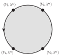
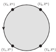
(a) 1342	(b) 1243	(c) 1234	(d) 1432

Figure 3: Disc amplitudes with two photon vertex operators ($V_{1}$ and $V_{2}$) and two tachyon vertex operators ($V_{3}$ and $V_{4}$) inserted. Kinematical amplitudes given by the disc amplitudes above are multiplied by the Chan–Paton factors $\mathop{\rm tr}[\lambda^{a_{1}}\lambda^{a_{3}}\lambda^{a_{4}}\lambda^{a_{2}}]$ in (a), $\mathop{\rm tr}[\lambda^{a_{1}}\lambda^{a_{2}}\lambda^{a_{4}}\lambda^{a_{3}}]$ in (b), $\mathop{\rm tr}[\lambda^{a_{1}}\lambda^{a_{2}}\lambda^{a_{3}}\lambda^{a_{4}}]$ in (c) and $\mathop{\rm tr}[\lambda^{a_{1}}\lambda^{a_{4}}\lambda^{a_{3}}\lambda^{a_{2}}]$ in (d), respectively. The two disc amplitudes (a, b) become ${\cal M}_{\rm Ven}(s,t)$, while (c, d) ${\cal M}_{\rm Ven}(u,t)$.

If the Chan–Paton matrices of a pair of incoming and outgoing vertex operators, $\lambda^{a_{1}}$ and $\lambda^{a_{2}}$, commute with each other, then the Chan–Paton factors from the diagrams Figure 3 (c, d) are the same, and the total kinematical part of the amplitude for this Chan–Paton factor becomes ${\cal M}_{\rm Ven}(s,t)+{\cal M}_{\rm Ven}(u,t)$.

Let us stay focused on ${\cal M}_{\rm Ven}(s,t)$ alone for now. The amplitude proportional to $\eta^{\mu\nu}$ can be expanded, as is well-known, as a sum only of $t$-channel poles:

$$\frac{g_{o}^{2}}{\alpha^{\prime}}\frac{\Gamma(-\alpha^{\prime}t-1)\Gamma(-\alpha^{\prime}s)}{\Gamma(-\alpha^{\prime}(s+t)-1)} = \frac{g_{o}^{2}}{\alpha^{\prime}}\int_{0}^{1}dx\;x^{-\alpha^{\prime}t-2}(1-x)^{-\alpha^{\prime}s-1},$$ (48)

$$= \frac{g_{o}^{2}}{\alpha^{\prime}}\sum_{N=0}^{\infty}\frac{-1}{\alpha^{\prime}t-(N-1)}\frac{(\alpha^{\prime}s+1)\cdots(\alpha^{\prime}s+N)}{N!}.$$ (49)

The Veneziano amplitude (4.2) can also be obtained in cubic string field theory [25]. In the cubic SFT, the scattering amplitude consists of two pieces, a collection of $t$-channel exchange diagrams and that of $s$-channel diagrams (Figure 4).

$${\cal M}_{\text{Ven}}(s,t)=\sum_{Y}{\cal M}^{(t)}_{Y}(s,t)+\sum_{Y}{\cal M}^{(s)}_{y}(s,t).$$ (50)

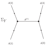
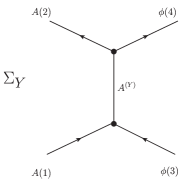
Figure 4: Two types of diagrams contribute to the photon–tachyon scattering amplitude ${\cal M}_{\rm Ven}(s,t)$ in cubic string field theory: $t$-channel exchange of one string states labeled by $Y$ (left), and $s$-channel exchange (right).

Infinitely many one string states (39) with zero ghost number ($h_{b}=h_{c}$)—labeled by $Y$—can be exchanged in the $t$-channel or in the $s$-channel, and the corresponding contributions are in the form of

$${\cal M}^{(t)}_{Y}=\frac{f^{(t)}_{Y}(s,t)}{-\alpha^{\prime}t-1+N^{(Y)}},\quad{\cal M}^{(s)}_{Y}=\frac{f^{(s)}_{Y}(t,s)}{-\alpha^{\prime}s-1+N^{(Y)}},$$ (51)

where $f^{(t)}_{Y}$ and $f^{(s)}_{Y}$ are regular function at finite $s,t$, and $N^{(Y)}$ is the excitation level (40) of a component field $A^{(Y)}$.

Because both the world-sheet calculation (4.2, 49) and the cubic SFT calculation (50, 51) are the same thing, ${\cal M}_{\rm Ven}(s,t)$ in both approaches should be completely the same functions of $(s,t)$. Therefore, for an arbitrary given value of $s$, the residue of all the poles in the complex $t$-plane should be the same. We also know that the Veneziano amplitude can be expanded purely in the infinite sum of $t$-channel poles with $t$-independent residues. This means that the full Veneziano amplitude (4.2) can be reproduced just from the $t$-channel cubic SFT amplitude $\sum_{Y}{\cal M}_{Y}^{(t)}(s,t)$, by the following procedure:

$$\sum_{Y}\frac{f^{(t)}_{Y}(s,t)}{-\alpha^{\prime}t-1+N^{(Y)}}\longrightarrow\sum_{Y}\frac{f^{(t)}_{Y}(s,(N^{(Y)}-1)/\alpha^{\prime})}{-\alpha^{\prime}t-1+N^{(Y)}}={\cal M}_{\rm Ven}(s,t).$$ (52)

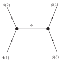
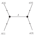
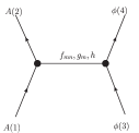
(a)	(b)	(c)

Figure 5: $t$-channel exchange diagrams for $A+\phi\rightarrow A+\phi$ scattering in the cubic string field theory. The tachyon ($N=0$), photon ($N=1$) and level-2 states are exchanged in the diagrams (a), (b) and (c), respectively.

To see that this prescription really works, let us take a look at the amplitudes of $t$-channel exchange of one string states with small excitation level $N^{(Y)}=0,1,2$. Focusing on the amplitude of $A+\phi\rightarrow A+\phi$ proportional to $\eta^{\mu\nu}$, we find that the tachyon exchange in the $t$-channel (Figure 5 (a)) gives rise to the amplitude [26]

$${\cal M}_{\phi}^{(t)}(s,t)=\left(\frac{g_{o}\lambda}{\alpha^{\prime}}\right)^{2}\left(\frac{2}{3^{3/4}}\right)^{-2\alpha^{\prime}t-2\alpha^{\prime}t+4}\frac{-1}{t+1/\alpha^{\prime}}=\frac{g_{o}^{2}}{\alpha^{\prime}}\left(\frac{27}{16}\right)^{\alpha^{\prime}t+1}\frac{-1}{\alpha^{\prime}t+1},$$ (53)

which is obtained simply by using the $\phi$-$\phi$-$\phi$ vertex rule (43) and $A$-$A$-$\phi$ vertex rule (45). The prescription (52) turns this amplitude into

$$\longrightarrow{\cal M}_{\phi}(s,t)=\frac{g_{o}^{2}}{\alpha^{\prime}}\frac{-1}{\alpha^{\prime}t+1},$$ (54)

which reproduces the $N=0$ term of (49).

The $t$-channel exchange of level $N^{(Y)}=1$ excited states can also be calculated in the cubic string field theory (Figure 5 (b)). The amplitude proportional to $\eta^{\mu\nu}$ is

$${\cal M}^{(t)}_{A}(s,t)=\frac{g_{o}^{2}}{\alpha^{\prime}}\left(\frac{27}{16}\right)^{\alpha^{\prime}t}\frac{-1}{\alpha^{\prime}t}\;\left[\frac{\alpha^{\prime}(s-u)}{2}\right],$$ (55)

where $(s-u)=(k_{(1)}-k_{(2)})\cdot(k_{(4)}-k_{(3)})$. Using the relation $\alpha^{\prime}(s+t+u)=-2$ in the tachyon–photon scattering to eliminate $u$ in favor of $s$ and $t$, and following the prescription (52)—which is to exploit $\alpha^{\prime}t=0$ in the numerator, this amplitude is replaced by [26]

$$\longrightarrow{\cal M}_{A}(s,t)=\frac{g_{o}^{2}}{\alpha^{\prime}}\frac{-(\alpha^{\prime}s+1)}{\alpha^{\prime}t}.$$ (56)

Once again, this reproduces the level $N=1$ contribution to the Veneziano amplitude (49).

Similar calculation for level-2 state exchange can be carried out (Figure 5 (c)). Using the vertex rule in (43) for the [level-2]-$\phi$-$\phi$ couplings, and also the interactions among [level-2]-$A$-$A$ coupling in the literature, the cubic SFT $t$-channel amplitude is given by [26]

$${\cal M}_{f}^{(t)}(s,t) = \frac{g_{o}^{2}}{\alpha^{\prime}}\left(\frac{27}{16}\right)^{\alpha^{\prime}t-1}\frac{-1}{\alpha^{\prime}t-1}\;\left[\frac{(\alpha^{\prime}(s-u))^{2}}{8}-\frac{5(\alpha^{\prime}t+2)}{16\cdot 2}+\frac{490}{16^{2}\cdot 2}\right],$$ (57)

$${\cal M}_{g}^{(t)}(s,t) = \frac{g_{o}^{2}}{\alpha^{\prime}}\left(\frac{27}{16}\right)^{\alpha^{\prime}t-1}\frac{-1}{\alpha^{\prime}t-1}\;\left[-\frac{36\;\alpha^{\prime}t}{16^{2}}\right],$$ (58)

$${\cal M}_{h}^{(t)}(s,t) = \frac{g_{o}^{2}}{\alpha^{\prime}}\left(\frac{27}{16}\right)^{\alpha^{\prime}t-1}\frac{-1}{\alpha^{\prime}t-1}\;\left[-\frac{11^{2}}{16^{2}}\right].$$ (59)

After using $\alpha^{\prime}u=-\alpha^{\prime}(s+t)-2$ to eliminate $u$ in favor of $s$ and $t$, and further following the prescription (52) [$\alpha^{\prime}t\rightarrow 1$ in the numerator], one will see that the level $N^{(Y)}=2$ amplitude turns into

$$\longrightarrow\left({\cal M}_{f}+{\cal M}_{g}+{\cal M}_{h}\right)(s,t)=\frac{g_{o}^{2}}{\alpha^{\prime}}\frac{-1}{\alpha^{\prime}t-1}\left[\frac{(\alpha^{\prime}s)^{2}+3(\alpha^{\prime}s)+2}{2}\right].$$ (60)

Once again, this is precisely the same as the $N=2$ contribution to the Veneziano amplitude (49).

Contributions from the $t$-channel exchange of states in the leading trajectory can also be examined systematically. Using the vertex rule (45, 46) involving the states in the leading trajectory ($Y=\left\{1^{N},0,0\right\}$), one finds that the amplitude proportional to $\eta^{\mu\nu}$ is

$${\cal M}_{\left\{1^{N},0,0\right\}}^{(t)}\simeq\frac{g_{o}^{2}}{\alpha^{\prime}}\left(\frac{27}{16}\right)^{\alpha^{\prime}t-(N-1)}\frac{-1}{\alpha^{\prime}t-(N-1)}\frac{\left(\alpha^{\prime}(s-u)/2\right)^{N}}{N!},$$ (61)

where we maintained only the terms with the highest power of either $s$ or $u$. After using the kinematical relation $\alpha^{\prime}(s+t+u)+2=0$ to eliminate $u$ in favor of $s$ and $t$, and following the prescription (52) [$\alpha^{\prime}t\rightarrow(N-1)$ in the numerator], we obtain the large-$\alpha^{\prime}s$ leading power contribution to the $N$-th term of (49) precisely with the correct coefficient.

We have therefore seen that the prescription (52) allows us to use the $t$-channel exchange amplitude in the cubic string field theory to construct the full disc scattering amplitude. In part II [5], this prescription is extended for the disc scattering amplitudes on a spacetime with curved background metric, which is the situation of real interest in the context of hadron scattering.

5 Mode Decomposition on AdS₅

Let us now proceed to work out mode decomposition of the totally symmetric (traceless) component field on the warped spacetime. The correspondence between the primary operators of the conformal field theory on the (UV) boundary and wavefunctions on AdS₅ is made clear. The Pomeron/Reggeon wavefunctions are obtained as a holomorphic function of the spin variable $j$, as we need to do so for the further inverse Mellin transformation. The wavefunction will then be used also to construct the scattering amplitude of $h+\gamma^{(*)}\rightarrow h+\gamma$ in our future publication [5].

Let the bilinear (free) part of the (bulk) action of a rank-$j$ tensor field on $AdS_{5}$ to be

$$S = -\frac{1}{2}\frac{t_{y}}{R^{3}}\int d^{4}x\int dz\sqrt{-g(z)}g^{m_{1}n_{1}}\cdots g^{m_{j}n_{j}}$$ (62)

$$\qquad\qquad\left[g^{m_{0}n_{0}}(\nabla_{m_{0}}A^{(y)}_{m_{1}\cdots m_{j}})(\nabla_{n_{0}}A^{(y)}_{n_{1}\cdots n_{j}})+\left(\frac{c_{y}}{R^{2}}+\frac{N^{(y)}_{\rm eff.}}{\alpha^{\prime}}\right)A^{(y)}_{m_{1}\cdots m_{j}}A^{(y)}_{n_{1}\cdots n_{j}}\right],$$

where we assume that kinetic mixing between different fields is either absent or sufficiently small. Here, the dimensionless parameter $N^{(y)}_{\rm eff.}$ is $N^{(Y)}-1$ for an $N^{(Y)}\in{\bf Z}_{\geq 0}$ for bosonic open string ($j\leq N^{(Y)}$), which would be $4(N^{(Y)}-1)$ for an $N^{(Y)}\in{\bf Z}_{\geq 1}$ for closed string ($j\leq 2N^{(Y)}$). This field is regarded as a reduction of some field with some “spherical harmonics” on the internal manifold, and hence $j\leq h_{a}$ in general. Another dimensionless coefficient $c_{y}$ may contain a contribution from the “mass” associated with the “spherical harmonics” over the internal manifold, and also include ambiguity (which is presumably of order unity) associated with making d’Alembertian of the flat metric background covariant.

The equation of motion (in the bulk part) then becomes

$$g^{m_{1}m_{2}}(\nabla_{m_{1}}\nabla_{m_{2}}A^{(y)}_{n_{1}\cdots n_{j}})-\left(\frac{c_{y}}{R^{2}}+\frac{N^{(y)}_{\rm eff.}}{\alpha^{\prime}}\right)A^{(y)}_{n_{1}\cdots n_{j}}=0.$$ (63)

Solutions to this equation of motion can be obtained from solutions of the following eigenmode equation

$$\nabla^{2}A_{m_{1}\cdots m_{j}}=-\frac{{\cal E}}{R^{2}}A_{m_{1}\cdots m_{j}},$$ (64)

by imposing the on-shell condition

$$\frac{({\cal E}+c_{y})}{\sqrt{\lambda}}+N^{(y)}_{\rm eff.}=0.$$ (65)

We will work out the eigenmode decomposition for rank-$j$ tensor fields in the following, where we only have to work for separate $j$, without referring to the mass parameter.

The eigenmode wavefunctions are used not just for constructing solutions to the equation of motions, but also in constructing the Reggeon exchange contributions to the $h+\gamma^{*}\rightarrow h+\gamma^{(*)}$ scattering amplitude. The propagator is proportional to

$$\frac{-i}{\frac{{\cal E}+c_{y}}{\sqrt{\lambda}}+N^{(y)}_{\rm eff.}-i\epsilon}\frac{\alpha^{\prime}R^{3}}{t_{y}}.$$ (66)

The mode equation for a rank-$j$ tensor field $A_{m_{1}\cdots m_{j}}$ on AdS₅ is further decomposed into those of irreducible representations of $SO(4,1)$. For simplicity of the argument, we only deal with the mode equations for the totally symmetric (and traceless) rank$-j$ tensor fields. Namely,

$$A_{m_{1}\cdots m_{j}}=A_{m_{\sigma(1)}\cdots m_{\sigma(j)}}\qquad\qquad{\rm for~{}}{}^{\forall}\sigma\in\mathfrak{S}_{j}.$$ (67)

We call them spin-$j$ fields.

The eigenmode equation (64) for a totally symmetric spin $j$ field can be decomposed into $j+1$ pieces, labeled by $k=0,\cdots,j$:

$$\left((R^{2}\Delta_{j})-\left[(2k+1)j-2k^{2}+3k\right]\right)A_{z^{k}\mu_{1}\cdots\mu_{j-k}}$$

$$+2zk\partial^{\hat{\rho}}A_{z^{k-1}\rho\mu_{1}\cdots\mu_{j-k}}+k(k-1)A^{\hat{\rho}}_{z^{k-2}\rho\mu_{1}\cdots\mu_{j-k}}$$

$$-2z(D[A_{z^{k+1}\cdots}])_{\mu_{1}\cdots\mu_{j-k}}+(E[A_{z^{k+2}\cdots}])_{\mu_{1}\cdots\mu_{j-k}}=-{\cal E}A_{z^{k}\mu_{1}\cdots\mu_{j-k}}.$$ (68)

Here,

$$A_{z^{k}\mu_{1}\cdots\mu_{j-k}}:=A_{\underbrace{z\cdots z}_{k}\mu_{1}\cdots\mu_{j-k}},$$ (69)

and can be regarded as a rank-$(j-k)$ totally symmetric tensor of $\mathop{\rm SO}(3,1)$ Lorentz group. $D[a]$ and $E[a]$ are operations creating totally symmetric rank-$(r+1)$ and rank-$(r+2)$ tensors of $\mathop{\rm SO}(3,1)$, respectively, from a totally symmetric rank-$r$ tensor of $\mathop{\rm SO}(3,1)$, $a$;

$$\left(D[a]\right)_{\mu_{1}\cdots\mu_{r+1}} := \sum_{i=1}^{r+1}\partial_{\mu_{i}}a_{\mu_{1}\cdots\check{\mu_{i}}\cdots\mu_{r+1}},$$ (70)

$$\left(E[a]\right)_{\mu_{1}\cdots\mu_{r+2}} := 2\sum_{p<q}\eta_{\mu_{p}\mu_{q}}a_{\mu_{1}\cdots\check{\mu_{p}}\cdots\check{\mu_{q}}\cdots\mu_{r+2}}.$$ (71)

The differential operator $\Delta_{j}$ in the first term is defined, as in [3], by

$$R^{2}\Delta_{j} := R^{2}z^{-j}\left[\left(\frac{z}{R}\right)^{5}\partial_{z}\left[\left(\frac{R}{z}\right)^{3}\partial_{z}\right]\right]z^{j}+R^{2}\left(\frac{z}{R}\right)^{2}\partial^{2},$$ (72)

$$= z^{2}\partial_{z}^{2}+(2j-3)z\partial_{z}+j(j-4)+z^{2}\partial^{2}.$$

The eigenmode equation (64, 68) is a generalization of the “Schrödinger equation” of [3] determining the Pomeron wavefunction. As we will see, the single-component Pomeron wavefunction discussed in [3] etc. corresponds to (100)—that of $(n,l,m)=(0,0,0)$ eigenmode in our language, and the Schrödinger equation to (97, 138); there are other eigenmodes, whose wavefunctions are to be determined in the following.

In the following sections 5.1–5.2, we simply state the results of the eigenmode decomposition of (64, 68) for spin-$j$ fields. More detailed account is given in the appendix A.

5.1 Eigenvalues and Eigenmodes for $\Delta^{\mu}=0$

Because of the 3+1-dimensional translational symmetry in $\nabla^{2}$, solutions to the eigenmode equations can be classified by the eigenvalues of the generators of translation, $(-i\partial^{\mu})$. Until the end of section 5.2, we will focus on eigenmodes in the form of

$$A_{m_{1}\cdots m_{j}}(x,z)=e^{i\Delta\cdot x}A_{m_{1}\cdots m_{j}}(z;\Delta),$$ (73)

and study the eigenmode equation (64) separately for different eigenvalues $\Delta^{\mu}$.

The eigenmode equation for $\Delta^{\mu}=0$ and that for $\Delta^{\mu}\neq 0$ are qualitatively different, and need separate study. The eigenmodes for $\Delta^{\mu}\neq 0$ will be presented in Section 5.2 (and appendix A.2); we begin in section 5.1 (and appendix (A.1)) with the eigenmode equations for $\Delta^{\mu}=0$, which is also regarded as an approximation of the eigenmode equation for $\Delta^{\mu}\neq 0$ in the asymptotic UV boundary region (at least $\Delta z\ll 1$, and maybe $z$ is as small as $R$).

For now, we relax the traceless condition on the spin-$j$ field $A_{m_{1}\cdots m_{j}}$ ($m_{i}=0,1,\cdots,3,z$), and we just assume that the rank-$j$ tensor field $A_{m_{1}\cdots m_{j}}$ is totally symmetric. Consider the following decomposition of the space of $z$-dependent field configuration $A_{m_{1}\cdots m_{j}}(z;\Delta=0)$:

$$A_{z^{k}\mu_{1}\cdots\mu_{j-k}}(z;\Delta^{\mu}=0)=\sum_{N=0}^{[(j-k)/2]}\left(E^{N}[a^{(k,N)}]\right)_{\mu_{1}\cdots\mu_{j-k}};$$ (74)

here, $\left(a^{(k,N)}(z;\Delta^{\mu}=0)\right)_{\mu_{1}\cdots\mu_{j-k-2N}}$ is a rank-$(j-k-2N)$ totally symmetric tensor of $\mathop{\rm SO}(3,1)$, and satisfies the 4D-traceless condition,

$$\eta^{\mu_{1}\mu_{2}}a^{(k,N)}_{\mu_{1}\cdots\mu_{j-k-2N}}=0.$$ (75)

Thus, the field configuration can be described by $a^{(k,N)}$’s with $0\leq k\leq j$, $0\leq N\leq[(j-k)/2]$. These components form groups labeled by $n=0,\cdots,j$, where the $n$-th group consists of $a^{(k,N)}$’s with $k+2N=n$; they are all rank-$(j-n)$ totally symmetric tensors of $\mathop{\rm SO}(3,1)$; let us call the subspace spanned by the components in this $n$-th group as the $n$-th subspace. The eigenmode equation for $\Delta^{\mu}=0$ becomes block diagonal under the decomposition into the subspaces labeled by $n=0,\cdots,j$. (See (A.1) in the appendix.) Therefore, the eigenmode equation for $\Delta^{\mu}=0$ can be studied separately for the individual $n$-th diagonal block.

The $n$-th diagonal block contains $[n/2]+1$ components, and hence there are $[n/2]+1$ eigenmodes. Let ${\cal E}_{n,l}$ ($l=0,\cdots,[n/2]$) be the eigenvalues in the $n$-th diagonal block. The corresponding eigenmode wavefunction is of the form

$$\left(a^{(k,N)}(z;\Delta^{\mu}=0)\right)_{\mu_{1}\cdots\mu_{j-n}}=c_{k,l,n}\;\left(\epsilon^{(n,l)}\right)_{\mu_{1}\cdots\mu_{j-n}}\;z^{2-j-i\nu},$$ (76)

where $\epsilon^{(n,l)}$ is a $z$-independent $k$-independent rank-$(j-n)$ tensor of $\mathop{\rm SO}(3,1)$. $c_{k,l,n}\in\mathbb{R}$. In the eigenmode equation for $\Delta^{\mu}=0$, the eigenmode wavefunctions are all in a simple power of $z$, and the power is parametrized by $i\nu$ ($\nu\in\mathbb{R}$). The eigenvalues ${\cal E}_{n,l}$ are functions of $\nu$; once the mass-shell condition (65) is imposed, the eigenmodes turn into solutions of the equation of motion, and $i\nu$ is determined by the mass parameter.

The eigenmodes with smaller $(n,l)$ are as follows:

$${\cal E}_{0,0}=(j+4+\nu^{2}), a^{(0,0)}(z)_{\mu_{1}\cdots\mu_{j}}=\epsilon^{(0,0)}_{\mu_{1}\cdots\mu_{j}}\;z^{2-j-i\nu},$$ (77)

$${\cal E}_{1,0}=(3j+5+\nu^{2}), a^{(1,0)}(z)_{\mu_{1}\cdots\mu_{j-1}}=\epsilon^{(1,0)}_{\mu_{1}\cdots\mu_{j-1}}z^{2-j-i\nu},$$ (78)

$${\cal E}_{2,0}=(5j+4+\nu^{2}), \left(\begin{array}[]{c}a^{(0,1)}(z)_{\mu_{1}\cdots\mu_{j-2}}\\ a^{(2,0)}(z)_{\mu_{1}\cdots\mu_{j-2}}\end{array}\right)=\left(\begin{array}[]{c}1\\ -4j\end{array}\right)\;\epsilon^{(2,0)}_{\mu_{1}\cdots\mu_{j-2}}\;z^{2-j-i\nu},$$ (83)

$${\cal E}_{2,1}=(j+2+\nu^{2}), \left(\begin{array}[]{c}a^{(0,1)}(z)_{\mu_{1}\cdots\mu_{j-2}}\\ a^{(2,0)}(z)_{\mu_{1}\cdots\mu_{j-2}}\end{array}\right)=\left(\begin{array}[]{c}1\\ 2\end{array}\right)\;\epsilon^{(2,1)}_{\mu_{1}\cdots\mu_{j-2}}\;z^{2-j-i\nu}.$$ (88)

Empirically, the $j$-dependence of the eigenvalues in the $n$-th diagonal block appear to be ${\cal E}_{n,l}=((2n+1-4l)j+\nu^{2}+O(1))$ ($l=0,\cdots,[n/2]$), [see (140–155) in the appendix for more samples of the eigenvalues] and we promote this $j$-dependence to a rule of the labeling of the eigenmodes with $l$.

The eigenmode with $l=0$ is found in any one of the $n$-th diagonal block ($n=0,\cdots,j$). Its eigenvalue is

$${\cal E}_{n,0}=(2n+1)j+2n-n^{2}+4+\nu^{2},$$ (89)

and

$$c_{2\bar{k},0,2\bar{n}}=(-)^{\bar{k}}4^{\bar{k}}\frac{\bar{n}!}{(\bar{n}-\bar{k})!}\frac{(j-\bar{n}+1)!}{(j-\bar{n}-\bar{k}+1)!}, (n=2\bar{n},\bar{k}=0,\cdots,\bar{n}),$$ (90)

$$c_{2\bar{k}+1,0,2\bar{n}+1}=(-)^{\bar{k}}4^{\bar{k}}\frac{\bar{n}!}{(\bar{n}-\bar{k})!}\frac{(j-\bar{n})!}{(j-\bar{n}-\bar{k})!}, (n=2\bar{n}+1,\bar{k}=0,\cdots,\bar{n}).$$ (91)

This $(n,l)=(n,0)$ eigenmodes are characterized by the 5D-traceless condition

$$g^{m_{1}m_{2}}A_{m_{1}\cdots m_{j}}=0.$$

Thus, the eigenmodes within the 5D-traceless (and totally symmetric) component—spin-$j$ field—for $\Delta^{\mu}=0$ are labeled simply by $n=0,\cdots,j$.

5.2 Mode Decomposition for non-zero $\Delta_{\mu}$

Diagonal Block Decomposition for the $\Delta^{\mu}\neq 0$ Case

The eigenmode equation (64, 68) is much more complicated in the case of $\Delta^{\mu}\neq 0$, because of the 2nd and 4th terms in (68). The eigenmode equation is still made block diagonal for an appropriate decomposition of the space of field $A_{m_{1}\cdots m_{j}}(z;\Delta^{\mu})$.

Consider a decomposition

$$A_{z^{k}\mu_{1}\cdots\mu_{j-k}}(z;\Delta^{\mu})=\sum_{s=0}^{j-k}\sum_{t=0}^{[s/2]}\left(\tilde{E}^{N}D^{s-2N}[a^{(k,s,N)}]\right)_{\mu_{1}\cdots\mu_{j-k}},$$ (92)

where a new operation $a\mapsto\tilde{E}[a]$ on a symmetric $\mathop{\rm SO}(3,1)$ tensor $a$,

$$\left(\tilde{E}[a]\right)_{\mu_{1}\cdots\mu_{r+2}}:=2\sum_{p<q}\left(\eta_{\mu_{p}\mu_{q}}-\frac{\partial_{\mu_{p}}\partial_{\mu_{q}}}{\partial^{2}}\right)a_{\mu_{1}\cdots\check{\mu_{p}}\cdots\check{\mu_{q}}\cdots\mu_{r+2}},$$ (93)

is used. $a^{(k,s,N)}$ are totally symmetric 4D-traceless (i.e. (75)) rank-$(j-k-s)$ tensor fields of $\mathop{\rm SO}(3,1)$ that satisfies an additional condition, the 4D-transverse condition:

$$\partial^{\hat{\rho}}\left(a^{(k,s,N)}\right)_{\rho\mu_{2}\cdots\mu_{j-k-s}}=i\Delta^{\hat{\rho}}\left(a^{(k,s,N)}\right)_{\rho\mu_{2}\cdots\mu_{j-k-s}}=0.$$ (94)

The space of field configuration $A_{m_{1}\cdots m_{j}}(z;\Delta^{\mu})$ is now decomposed into $a^{(k,s,N)}$’s with $0\leq k\leq j$, $0\leq s\leq j-k$, $0\leq N\leq[s/2]$; these components form groups labeled by $m=0,\cdots,j$, where the $m$-th group consists of $a^{(k,s,N)}$’s with $k+s=m$; they are all rank-$(j-m)$ totally symmetric 4D-traceless and 4D-transverse tensors of $\mathop{\rm SO}(3,1)$; let us call the subspace spanned by the components in this $m$-th group as the $m$-th subspace. The eigenmode equation for $\Delta^{\mu}\neq 0$ becomes block diagonal under the decomposition into the subspaces labeled by $m=0,\cdots,j$. The eigenmode equation for the $m$-th sector is given by (A.2) in the appendix A.2. The $m$-th subspace should have

$$\sum_{s=0}^{m}\left([s/2]+1\right)$$ (95)

eigenmodes.

Eigenvalues ${\cal E}$ are determined in terms of the characteristic exponent in the expansion of the solution in power series of $z$; let the first term in the expansion be $z^{2-j-i\nu}$; the eigenvalues are functions of $\nu$ then. Because the indicial equation at the regular singular point $z\simeq 0$ allows us to determine the eigenvalues in terms of $\nu$, the eigenvalues in the case of $\Delta^{\mu}\neq 0$ cannot be different from the ones we have already known in the $\Delta^{\mu}=0$ case. In the $m$-th diagonal block, the eigenvalues consist of ${\cal E}_{n,l}$ with $0\leq n\leq m$, $0\leq l\leq[n/2]$.

To summarize, the eigenmodes in the totally symmetric rank-$j$ tensor field of $\mathop{\rm SO}(4,1)$ are labeled by $(n,l,m)$ and $\Delta^{\mu}$ and $\nu$. Their eigenvalues ${\cal E}_{n,l}$ depend only on $n$ and $l$ (with $0\leq n\leq j$ and $0\leq l\leq[n/2]$) and $\nu$. Corresponding eigenmodes are denoted by

$$A(x,z)^{n,l,m;\Delta,\nu}_{z^{k}\mu_{1}\cdots\mu_{j-k}} =$$

$$e^{i\Delta\cdot x}A^{n,l,m}_{z^{k}\mu_{1}\cdots\mu_{j-k}}(z;\Delta^{\mu},\nu) = e^{i\Delta\cdot x}\sum_{N=0}^{[s/2]}\tilde{E}^{N}D^{s-2N}[\epsilon^{(n,l,m)}]\frac{b^{(j-m)}_{s,N}}{\Delta^{s-2N}}\Psi^{(j);s,N}_{i\nu;n,l,m}(-\Delta^{2},z).$$ (96)

$\epsilon^{(n,l,m)}$ is a ($z$-independent) totally symmetric 4D-traceless 4D-transverse rank-$(j-m)$ tensor of $\mathop{\rm SO}(3,1)$, and all the $s$’s appearing in the expression above are understood as $s=m-k$. $b^{(r)}_{s,N}$ is a constant whose definition is given in (171) in the appendix.

Single Component Pomeron Wavefunction

The Pomeron wavefunction that has been discussed in the literature (e.g. [3]) does not look as awful as (96). To our knowledge, the Pomeron wavefunction in the literature in the context of hadron high-energy scattering has been a single component one, $\Psi_{i\nu}(t,z)$. How is $A^{n,l,m}_{m_{1}\cdots m_{j}}(z;\Delta^{\mu},\nu)$ related to $\Psi_{i\nu}(-\Delta^{2};z)$?

In the block diagonal decomposition of the eigenmode equation, there is only one subspace where the diagonal block is $1\times 1$. That is the $m=0$ subspace, which consists only of $a^{(0,0,0)}$. The eigenmode equation is

$$\left[\Delta_{j}-\frac{j}{R^{2}}\right]a^{(0,0,0)}(z;\Delta^{\mu})=-\frac{{\cal E}}{R^{2}}a^{(0,0,0)}(z;\Delta^{\mu}).$$ (97)

This equation, as well as (138) in the $\Delta^{\mu}=0$ case, corresponds to the “Schrödinger equation” in [3] determining the Pomeron wavefunction. It should be noted, however, that we consider that $\nabla^{2}$ is the operator relevant to the eigenmode decomposition rather than $\Delta_{j}$; furthermore the operator $\nabla^{2}$ and $\Delta_{j}$ has a simple relation $\nabla^{2}=\Delta_{j}-j/R^{2}$ only on this $m=0$-th subspace of a totally symmetric rank-$j$ tensor field of $\mathop{\rm SO}(4,1)$.

The eigenvalue is

$${\cal E}_{0,0}=(j+4+\nu^{2}),$$ (98)

when we define the first term in the power series expansion of $z$ to be $z^{2-j-i\nu}$. The eigenmode wavefunction is

$$a^{(0,0,0)}(z;\Delta^{\mu})_{\mu_{1}\cdots\mu_{j}} = \epsilon^{(0,0,0)}_{\mu_{1}\cdots\mu_{j}}\;\Psi^{(j)}_{i\nu}(-\Delta^{2},z),$$ (99)

$$\Psi^{(j)}_{i\nu}(-\Delta^{2},z) := \frac{2}{\pi}\sqrt{\frac{\nu\sinh(\pi\nu)}{2R}}\;e^{(j-2)A}K_{i\nu}(\Delta z).$$ (100)

The normalization factor is determined [3] so that it satisfies the normalization condition

$$\int d^{4}x\int dz\sqrt{-g(z)}e^{-2jA}\;[e^{i\Delta\cdot x}\Psi^{(j)}_{i\nu}(-\Delta^{2},z)]\;[\Psi^{(j)}_{i\nu^{\prime}}(-\Delta^{{}^{\prime}2},z)e^{-i\Delta^{\prime}\cdot x}]=(2\pi)^{4}\delta^{4}(\Delta-\Delta^{\prime})\;\delta(\nu-\nu^{\prime}).$$ (101)

The single component Pomeron/Reggeon wavefunction $\Psi^{(j)}_{i\nu}(-\Delta^{2},z)$ is now understood as $\Psi^{(j);0,0}_{i\nu;0,0,0}(-\Delta^{2},z)$.

5D-Traceless 5D-Transverse Modes

The eigenmode equation (64) for a totally symmetric rank-$j$ tensor field of $\mathop{\rm SO}(4,1)$ should be closed within its 5D-traceless component. The subspace of 5D-traceless component is characterized by the 5D-traceless condition

$$g^{m_{1}m_{2}}A_{m_{1}\cdots m_{j}}(z;\Delta^{\mu})=0.$$ (102)

The fact that the Hermitian operator $\nabla^{2}$ maps this subspace to itself implies that the eigenmode equation of $\nabla^{2}$ is block diagonal, when the space of (not-necessarily 5D-traceless) $A_{m_{1}\cdots m_{j}}$ is decomposed into the sum of the 5D-traceless subspace and its orthogonal complement. Collection of the eigenmodes with $l=0$ correspond to the subspace of 5D-traceless field configuration.

Similarly, one can think of a subspace of field configuration satisfying both the 5D-traceless condition (102) and the 5D-transverse condition

$$g^{nm_{1}}\nabla_{n}A_{m_{1}m_{2}\cdots m_{j}}=0.$$ (103)

Obviously this is a subspace of the subspace of 5D-traceless modes we discussed above. Since the Hermitian operator $\nabla^{2}$ on AdS₅ maps this new subspace also to itself, the eigenmode equation of $\nabla^{2}$ should also become block diagonal, when the subspace of 5D-traceless modes is decomposed into this new subspace its orthogonal complement.

As we will see in the appendix A.3, there is only one such mode satisfying this set of conditions (102, 103) in each one of the $m$-th diagonal block. Thus, the combination of the 5D-traceless and 5D-transverse conditions allow us to determine an eigenmode completely. This mode turns out to be $(n,l,m)=(0,0,m)$ (for $0\leq m\leq j$). Put differently, the eigenmodes with the eigenvalue ${\cal E}_{n,l}={\cal E}_{0,0}=(j+4+\nu^{2})$ are charachterized by the traceless and transverse conditions on AdS₅.

The eigenmode wavefunctions of the 5D-traceless transverse modes $(n,l,m)=(0,0,m)$ are (see the appendix A.3)

$$\Psi^{(j);s,N}_{i\nu;0,0,m}(-\Delta^{2},z)=\sum_{a=0}^{N}(-)^{a}{}_{N}C_{a}\left(\frac{z^{3}\partial_{z}z^{-3}}{\Delta}\right)^{s-2a}\left[(z\Delta)^{m}\Psi^{(j);0,0}_{i\nu;0,0,0}(-\Delta^{2},z)\right]\times N_{j,m}.$$ (104)

$N_{j,m}$ is a dimensionless normalization constant. We choose it to be

$$N_{j,m}^{-2}={}_{j}C_{m}\frac{\Gamma(j+1-i\nu)}{\Gamma(j+1-m-i\nu)}\frac{\Gamma(j+1+i\nu)}{\Gamma(j+1-m+i\nu)}\frac{\Gamma(3/2+j-m)}{2^{m}\Gamma(3/2+j)}\frac{\Gamma(2+2j)}{\Gamma(2+2j-m)},$$ (105)

so that the eigenmode wavefunctions are normalized as in

$$\int d^{4}x\int_{0}dz\sqrt{-g(z)}g^{m_{1}n_{1}}\cdots g^{m_{j}n_{j}}\;A^{n,l,m;\Delta,\nu}_{m_{1}\cdots m_{j}}(x,z)\;A^{n^{\prime},l^{\prime},m^{\prime};\Delta^{\prime},\nu^{\prime}}_{n_{1}\cdots n_{j}}(x,z)$$ (106)

$$= (2\pi)^{4}\delta^{4}(\Delta+\Delta^{{}^{\prime}})\;\delta(\nu-\nu^{\prime})\;\delta_{n,n^{\prime}}\delta_{l,l^{\prime}}\delta_{m,m^{\prime}}\;\left[\epsilon^{(n,l,m)}(\Delta)\right]\cdot\left[\epsilon^{(n^{\prime},l^{\prime},m^{\prime})}(\Delta^{\prime})\right].$$

Here, $[\epsilon^{(n,l,m)}]\cdot[\epsilon^{{}^{\prime}(n,l,m)}]:=\epsilon^{(n,l,m)}_{\mu_{1}\cdots\mu_{j-m}}\epsilon^{{}^{\prime}(n,l,m)}_{\nu_{1}\cdots\nu_{j-m}}\eta^{\hat{\mu}_{1}\hat{\nu}_{1}}\cdots\eta^{\hat{\mu}_{j-m}\hat{\nu}_{j-m}}$.

Propagator

The propagator of the totally symmetric rank-$j$ tensor field [resp. spin-$j$ field] on AdS₅ is given by summing up propagators of the $(n,l,m)$ modes [resp. $(n,l,m)$ modes with $l=0$]. In order to write down the propagator of a given $(n,l,m)$ eigenmode, it is convenient to introduce the following notation:

$$A^{n,l,m;\Delta,\nu}_{m_{1}\cdots m_{j}}(x,z)=\left[A^{n,l,m;\Delta,\nu}_{m_{1}\cdots m_{j}}(x,z)\right]^{\hat{\kappa}_{1}\cdots\hat{\kappa}_{j-m}}\epsilon^{(n,l,m)}_{\kappa_{1}\cdots\kappa_{j-m}}=e^{i\Delta\cdot x}\left[A^{n,l,m}_{m_{1}\cdots m_{j}}(z;\Delta^{\mu},\nu)\right]^{\hat{\kappa}_{1}\cdots\hat{\kappa}_{j-m}}\epsilon^{(n,l,m)}_{\kappa_{1}\cdots\kappa_{j-m}}.$$ (107)

With this notation, the propagator of the $(n,l,m)$ mode is given by

$$G(x,z;x^{\prime},z^{\prime})_{m_{1}\cdots m_{j};n_{1}\cdots n_{j}}^{(n,l,m)} = \int\frac{d^{4}\Delta}{(2\pi)^{4}}\int_{0}^{\infty}d\nu\frac{-iP_{\rho_{1}\cdots\rho_{j-m};\;\sigma_{1}\cdots\sigma_{j-m}}}{\frac{{\cal E}_{n,l}+c}{\sqrt{\lambda}}+N_{\rm eff.}-i\epsilon}\frac{\alpha^{\prime}R^{3}}{C}$$ (108)

$$\left[A^{n,l,m;\Delta,\nu}_{m_{1}\cdots m_{j}}(x,z)\right]^{\rho_{1}\cdots\rho_{j-m}}\left[A^{n,l,m;-\Delta,\nu}_{n_{1}\cdots n_{j}}(x^{\prime},z^{\prime})\right]^{\sigma_{1}\cdots\sigma_{j-m}}.$$

Here, $P_{\rho_{1}\cdots\rho_{j-m};\;\sigma_{1}\cdots\sigma_{j-m}}$ is a polarization tensor generalizing $\eta_{\rho\sigma}-\partial_{\rho}\partial_{\sigma}/\partial^{2}$. When an orthogonal basis $\epsilon_{a}(q)\cdot\epsilon_{b}(-q)=\delta_{a,b}D_{a}$ of rank-$r$ 4D-traceless 4D-transverse tensors is given,

$$P_{\mu_{1}\cdots\mu_{r};\;\nu_{1}\cdots\nu_{r}}:=\sum_{a}\frac{1}{D_{a}}\epsilon(q)_{a;\;\mu_{1}\cdots\mu_{r}}\epsilon(-q)_{a;\;\nu_{1}\cdots\nu_{r}}.$$ (109)

An alternative characterization of this $P_{\mu_{1}\cdots\mu_{r};\nu_{1}\cdots\nu_{r}}$ is given by a combination of the two following conditions: one is

$$P_{\mu_{1}\cdots\mu_{r};\;\nu_{1}\cdots\nu_{r}}\epsilon_{a}^{\nu_{1}\cdots\nu_{r}}=\epsilon_{a;\mu_{1}\cdots\mu_{r}},$$ (110)

and the other is that $P_{\mu_{1}\cdots\mu_{r};\;\nu_{1}\cdots\nu_{r}}$ be also a totally symmetric 4D-transverse 4D-traceless tensor with respect to $(\mu_{1}\cdots\mu_{r})$ for any choice of $(\nu_{1}\cdots\nu_{r})$.

5.3 Representation in the Dilatation Eigenbasis

It is an essential process in the application of AdS/CFT correspondence to classify solutions to the equation of motions on the gravity dual background (AdS₅) into irreducible representations of the conformal group $\mathop{\rm SO}(4,2)$ (or possibly its supersymmetric extension). In the CFT description, primary operators are in one to one correspondence with (highest weight) irreducible representations of the conformal group, and it is believed that one can establish an one-to-one correspondce between i) a primary operator in the CFT description and ii) a group of solutions to the equation of motion forming an irreducible representation in the gravity dual description. Once this correspondence is given, then hadron matrix elements of the primary operators in a (nearly conformal) field theory can be calculated by using the corresponding solutions to the equation of motions (wavefunctions) on AdS₅. Note that the hadron matrix elements of primary operators are all that remains unknown in the formulation of conformal operator product expansion (26).

Let $P_{\mu}$, $K_{\mu}$, $L_{\mu\nu}$ and $D$ denote the generators of the unitary operators of the conformal group transformation on the Hilbert space. They satisfy the following commutation relations:

$$[D,P_{\mu}]=iP_{\mu}, [P_{\rho},L_{\mu\nu}]=i(\eta_{\rho\mu}P_{\nu}-\eta_{\rho\nu}P_{\mu}),$$ (111)

$$[D,K_{\mu}]=-iK_{\mu}, [K_{\rho},L_{\mu\nu}]=i(\eta_{\rho\mu}K_{\nu}-\eta_{\rho\nu}K_{\mu}),$$ (112)

$$[P_{\mu},K_{\nu}]=-2i(\eta_{\mu\nu}D+L_{\mu\nu}),$$ (113)

$$[L_{\mu\nu},L_{\rho\sigma}]=i(\eta_{\nu\rho}L_{\mu\sigma}-\eta_{\nu\sigma}L_{\mu\rho}-\eta_{\mu\rho}L_{\nu\sigma}+\eta_{\mu\sigma}L_{\nu\rho}).$$ (114)

When such a conformal symmetry exists in a conformal field thoery on 3+1 dimensions, those generators have a representation as differential operators on fields on $\mathbb{R}^{3,1}$; those differential operators are denoted by ${\cal P}_{\mu}$, ${\cal K}_{\mu}$, ${\cal L}_{\mu\nu}$ and ${\cal D}$. The generators and the differential operators on a CFT are in the following relation:

$$[{\cal O}(x),P_{\mu}]={\cal P}_{\mu}{\cal O}(x),\quad[{\cal O}(x),K_{\mu}]={\cal K}_{\mu}{\cal O}(x),\quad[{\cal O}(x),D]={\cal D}{\cal O}(x),\cdots,$$ (115)

and those differential operators acts on primary operators as follows:

$${\cal D}\overline{\cal O}_{n}(x) = -i(x\cdot\partial+l_{n})\overline{\cal O}_{n}(x),$$ (116)

$${\cal L}_{\mu\nu}\overline{\cal O}_{n}(x) = \left(i(x_{\mu}\partial_{\nu}-x_{\nu}\partial_{\mu})+[S_{\mu\nu}]\right)\overline{\cal O}_{n}(x)$$ (117)

$${\cal P}_{\mu}\overline{\cal O}_{n}(x) = -i\partial_{\mu}\overline{\cal O}_{n}(x),$$ (118)

$${\cal K}_{\mu}\overline{\cal O}_{n}(x) = \left(-i(2x_{\mu}x\cdot\partial-x^{2}\partial_{\mu})-i2l_{n}x_{\mu}-x^{\kappa}[S_{\mu\nu}]\right)\overline{\cal O}_{n}(x),$$ (119)

where $[S_{\mu\nu}]$ is a finite dimensional representation of $\mathop{\rm SO}(3,1)$ generators satisfying the same commutation relation as $L_{\mu\nu}$’s. Thus, for a primary operator $\overline{\cal O}_{n}(x)$, $\overline{\cal O}_{n}(x=0)$ plays the role of the highest weight state

$$[\overline{\cal O}_{n}(0),K_{\mu}]=0,\qquad[\overline{\cal O}_{n}(0),D]=-il_{n}\overline{\cal O}_{n}(0);$$ (120)

all other states in the highest weight state representation—decendants—are generated by applying $[\bullet,P_{\mu}]$ multiple times; the whole representation, therefore, is spanned by a collection of

$$\left\{\overline{\cal O}_{n}(0),\;\partial_{\mu}\overline{\cal O}_{n}(0),\;\partial_{\mu}\partial_{\nu}\overline{\cal O}_{n}(0),\;\cdots\right\};$$ (121)

it is also equivalent to $\overline{\cal O}(x=x_{0})$ with arbitrary $x_{0}\in\mathbb{R}^{3,1}$.

In the preceding sections, we have worked on solutions to the eigenmode equation on AdS₅; once the mass-shell condition (65) is imposed, they become solutions to the equation of motion. They are obtained as an eigenmode of the spacetime translation in 3+1 dimensions, $(-i\partial^{\mu})=\Delta^{\mu}$. Under the conformal group $\mathop{\rm SO}(4,2)$, which contains Lorentz $\mathop{\rm SO}(3,1)$ symmetry, however, an irreducible representation has to include solutions with all kinds of eiganvalues $\Delta^{\mu}$.

In the case of a scalar field on AdS₅, one can think of the following linear combination $G(x,z;x_{0};R_{0})$ (for some $R_{0}\ll\Delta^{-1}$):

$$G(x,z;x_{0})=\frac{i}{\pi^{2}}\frac{\Gamma(l_{n})}{\Gamma(l_{n}-2)}R_{0}^{l_{n}-4}\left(\frac{z}{z^{2}+(x-x_{0})^{2}}\right)^{l_{n}}=\int\frac{d^{4}\Delta}{(2\pi)^{4}}e^{i\Delta\cdot(x-x_{0})}\frac{(\Delta z)^{2}K_{l_{n}-2}(\Delta z)}{(\Delta R_{0})^{2}K_{l_{n}-2}(\Delta R_{0})}.$$ (122)

The factor $[e^{i\Delta\cdot x}(\Delta z)^{2}K_{l_{n}-2}(\Delta z)]$ in the integrand on the right hand side is a solution to the equation of motion of a scalar field on AdS₅ whose mass-square $M^{2}_{\rm eff.}$ is given by $l_{n}-2=i\nu=\sqrt{4+M^{2}_{\rm eff.}R^{2}}$. The coefficient of the linear combination, $e^{-i\Delta\cdot x_{0}}[(\Delta R_{0})^{2}K_{l_{n}-2}(\Delta R_{0})]$, is chosen so that the integrand behaves as

$$e^{i\Delta\cdot(x-x_{0})}\left(\frac{z}{R_{0}}\right)^{4-l_{n}}$$ (123)

at $0\leq z\ll\Delta^{-1}$. The space of solutions to the equation of motion parametrized by $x_{0}\in\mathbb{R}^{3,1}$ is spanned by derivatives of $G(x,z;x_{0})$ with respect to $x^{\mu}_{0}$ at $x^{\mu}_{0}=0$. It is easy to see that this basis

$$\left\{G(x,z;0),\;\partial^{(x_{0})}_{\mu}G(x,z;0),\;\partial^{(x_{0})}_{\mu}\partial^{(x_{0})}_{\nu}G(x,z;0),\;\cdots\right\}$$ (124)

is an eigenbasis under the action of dilatation, ${\cal D}:=i(z\partial_{z}+x\cdot\partial)$, and their weights are $-il_{n}$, $-i(l_{n}+1)$, $-i(l_{n}+2),\cdots$, respectively. Correspondence between scalar field wavefunctions on AdS₅ and scalar primary operators of the dual CFT is established in this way [27].

Let us now generalize the discussion above slightly, to construct an analogue of $G(x,z;x_{0})$ for a spin-$j$ field $A_{m_{1}\cdots m_{j}}$ on AdS₅, from which the dilatation eigenbasis is constructed. To this end, note that all the $(0,0,m)$-modes ($m=0,\cdots,j$) have the leading $z^{2-j-i\nu}$ in the power series expansion only in the $A_{z^{0}\mu_{1}\cdots\mu_{j}}$ component, not in any other $A_{z^{k}\mu_{1}\cdots\mu_{j-k}}$ components with $k>0$. It is possible to choose $\epsilon^{(0,0,m)}(\Delta^{\mu})$ properly so that

$$\sum_{m=0}^{j}\left[A^{0,0,m;\Delta,\nu}_{\mu_{1}\cdots\mu_{j}}(x,z)\right]^{\hat{\kappa}_{1}\cdots\hat{\kappa}_{j-m}}\epsilon^{(0,0,m)}_{\kappa_{1}\cdots\kappa_{j-m}}e^{-i\Delta\cdot x_{0}}\simeq e^{i\Delta\cdot(x-x_{0})}\left(\frac{z}{R_{0}}\right)^{2-j-i\nu}\epsilon_{\mu_{1}\cdots\mu_{j}}$$ (125)

in the region near the UV boundary $z\ll\Delta^{-1}$, where $\epsilon_{\mu_{1}\cdots\mu_{j}}$ is a $\Delta^{\mu}$-independent 4D-traceless totally symmetric rank-$j$ tensor of $\mathop{\rm SO}(3,1)$. The condition is

$$\epsilon_{\mu_{1}\cdots\mu_{j}} = \left(\frac{R_{0}}{R}\right)^{2-j}\!\!\!\!\!K_{i\nu}(\Delta R_{0})\frac{2}{\pi}\sqrt{\frac{\nu\sinh(\pi\nu)}{2R}}$$ (126)

$$\sum_{m=0}^{j}\frac{N_{j,m}\Gamma(m-j-i\nu)}{\Gamma(-j-i\nu)}\sum_{N=0}^{[m/2]}\frac{b^{(j-m)}_{m,N}}{\Delta^{m-2N}}\left(\tilde{E}^{N}D^{m-2N}[\epsilon^{(0,0,m)}]\right)_{\mu_{1}\cdots\mu_{j}}$$

It is possible to invert this relation by using (170) and write down $\epsilon^{(0,0,m)}(\Delta^{\mu})$ in terms of $\epsilon_{\mu_{1}\cdots\mu_{j}}$, though we will not present the result here. What really matters to us is that $\epsilon^{(0,0,m)}(\lambda\Delta)=\epsilon^{(0,0,m)}(\Delta)\lambda^{i\nu}$. With $\epsilon^{(0,0,m)}$’s satisfying the condition above, one can see that the following linear combination of solutions to the equation of motion,

$$G_{m_{1}\cdots m_{j}}(x,z;x_{0}):=\int\frac{d^{4}\Delta}{(2\pi)^{4}}\sum_{m=0}^{j}\left[A^{0,0,m;\Delta,\nu}_{m_{1}\cdots m_{j}}(x,z)\right]^{\hat{\kappa}_{1}\cdots\hat{\kappa}_{j-m}}\epsilon^{(0,0,m)}(\Delta)_{\kappa_{1}\cdots\kappa_{j-m}}e^{-i\Delta\cdot x_{0}},$$ (127)

has a property

$$G_{m_{1}\cdots m_{j}}(\lambda x,\lambda z;\lambda x_{0})=\lambda^{-(2+j+i\nu)}G_{m_{1}\cdots m_{j}}(x,z;x_{0}).$$ (128)

$i\nu$ is determined by the mass parameter on AdS₅, once the mass shell condition (65) is imposed. Therefore, $G_{m_{1}\cdots m_{j}}(x,z;0)$ is an eigenstate of dilatation, and so are the derivatives of $G_{m_{1}\cdots m_{j}}(x,z;x_{0})$ with respect to $x_{0}^{\mu}$ at $x_{0}^{\mu}=0$. All the derivatives combined form a dilatation eigenbasis in the space of solutions to the equation of motion of a spin-$j$ field.

It is now clear that the eigenmodes with $(n,l,m)=(0,0,m)$ ($0\leq m\leq j$) and arbitrary $\Delta^{\mu}$ as a whole—modes that satisfy the 5D-traceless and 5D-transverse conditions (102, 103)—forms an irreducible representation of the conformal group. If one is interested purely in the matrix element of a spin-$j$ primary operator $\overline{\cal O}_{n}(x_{0}=0)$ of an approximately conformal gauge theory, then the matrix element can be calculated by using the wavefunction $G_{m_{1}\cdots m_{j}}(x,z;0)$. Note that the $m=0$ mode alone, where the Pomeron/Reggeon wavefunction has a single component as in [3], cannot reproduce all the matrix element associated with matrix elements of spin-$j$ primary operators.

Appendix A More on the Mode Decomposition on AdS₅

For convenience, let us copy here the eigenmode equation (64) for a totally symmetric rank-$j$ tensor field on AdS₅; the equation consists of the following equations labeled by $k=0,\cdots,j$:

$$\left((R^{2}\Delta_{j})-\left[(2k+1)j-2k^{2}+3k\right]\right)A_{z^{k}\mu_{1}\cdots\mu_{j-k}}$$

$$+2zk\partial^{\hat{\rho}}A_{z^{k-1}\rho\mu_{1}\cdots\mu_{j-k}}+k(k-1)A^{\hat{\rho}}_{z^{k-2}\rho\mu_{1}\cdots\mu_{j-k}}$$

$$-2z(D[A_{z^{k+1}\cdots}])_{\mu_{1}\cdots\mu_{j-k}}+(E[A_{z^{k+2}\cdots}])_{\mu_{1}\cdots\mu_{j-k}}=-{\cal E}A_{z^{k}\mu_{1}\cdots\mu_{j-k}}.$$ (129)

A.1 Eigenvalues and Eigenmodes for $\Delta^{\mu}=0$

block diagonal decomposition

In the main text, we considered a decomposition of the rank-$j$ totally symmetric tensor field with $(-i\Delta_{\mu})=\Delta_{\mu}=0$ in the form of

$$A_{z^{k}\mu_{1}\cdots\mu_{j-k}}(z;\Delta^{\mu}=0)=\sum_{N=0}^{[(j-k)/2]}\left(E^{N}[a^{(k,N)}]\right)_{\mu_{1}\cdots\mu_{j-k}};$$

where $a^{(k,N)}$’s are $z$-dependent rank-$(j-k-2N)$ totally symmetric tensor field of $\mathop{\rm SO}(3,1)$, satisfying the 4D-traceless condition (75). This is indeed a decomposition, in that all the degrees of freedom in $A_{z^{k}\mu_{1}\cdots\mu_{j}-k}(z;\Delta^{\mu}=0)$ are described by $a^{(k,N)}(z)_{\mu_{1}\cdots\mu_{j-k-2N}}$ with $0\leq N\leq[(j-k)/2]$ without redundancy. To see this, one only needs to note that there is a relation that, for a totally symmetric 4D-traceless rank-$r$ $\mathop{\rm SO}(3,1)$-tensor $a$,

$$\eta^{\hat{\rho}\hat{\sigma}}E^{N}[a]_{\rho\sigma\mu_{1}\cdots\mu_{r+2N-2}}=4N(r+N+1)E^{N-1}[a]_{\mu_{1}\cdots\mu_{r+2N-2}}.$$ (130)

Using this relation, $a^{(k,N)}_{\mu_{1}\cdots\mu_{j-k-2N}}$ can be retrieved from $A_{z^{k}\mu_{1}\cdots\mu_{j-k}}$, starting from ones with larger $N$ to ones with smaller $N$.

Let us now see that the eigenmode equation (68=129) can be made block diagonal by using this decomposition. The eigenmode equation (129) with the label $k$ for $\Delta^{\mu}=0$ can be rewritten by using this relation (130) as follows:

$$\sum_{N} \left(R^{2}\Delta_{j}-\left[(2k+1)j-2k^{2}+3k\right]+{\cal E}\right)E^{N}[a^{(k,N)}]$$

$$+ k(k-1)\left[4(N+1)(j-k-N+2)\right]E^{N}[a^{(k-2,N+1)}]+E[E^{N-1}[a^{(k+2,N-1)}]]=0.$$

Although this equation has to hold only after the summation in $N$, it actually has to be satisfied separately for different $N$’s. To see this, let us first multiply $\eta^{\hat{\rho}\hat{\sigma}}$ for $[(j-k)/2]$ times and contract indices just like in (130); we obtain an equation that involves only $a^{k,[(j-k)/2]}$, $a^{(k-2,[(j-k)/2]+1)}$ and $a^{(k+2),[(j-k)/2]-1}$. Next, multiply $\eta^{\hat{\rho}\hat{\sigma}}$ for $[(j-k)/2]-1$ times, to obtain another eqution involving $a^{k,[(j-k)/2]-1}$, $a^{(k-2,[(j-k)/2])}$ and $a^{(k+2),[(j-k)/2]-2}$. In this way, we obtain

$$\left(R^{2}\Delta_{j}-\left[(2k+1)j-2k^{2}+3k\right]+{\cal E}\right)a^{(k,N)}$$

$$+ k(k-1)\left[4(N+1)(j-k-N+2)\right]a^{(k-2,N+1)}+a^{(k+2,N-1)}=0.\qquad\qquad({\rm for~{}}{}^{\forall}k,N)$$

Fields $a^{(k,N)}$’s with the same $k+2N=n$ form a system of coupled equations, but those with different $n=k+2N$ do not mix. Thus, the eigenmode equation for $\Delta^{\mu}=0$ is decomposed into sectors labeled by $n$. The $n$-th sector consists of $z$-dependent fields that are all in the rank-$(j-n)=(j-k-2N)$ totally symmetric tensor of $\mathop{\rm SO}(3,1)$.

classification of eigenmodes for $\Delta^{\mu}=0$

Let us now study the eigenmode equations more in detail for the separate diagonal blocks we have seen. Simultaneous treatmen is possible for all the $n$-th sectors with even $n$, and for all the sectors with odd $n$.

Let us first look at the $n$-th sector of the eigenmode problem for an $n=2\bar{n}\leq j$. In the eigenmode equation of $\Delta^{\mu}=0$, we can assume the same $z$-dependence for all the fields in this diagonal block:

$$a^{(k,N)}(z)_{\mu_{1}\cdots\mu_{j-n}}=\bar{a}^{(k,N)}_{\mu_{1}\cdots\mu_{j-n}}z^{2-j-i\nu},\qquad\qquad k+2N=n$$ (132)

where $\bar{a}^{(k,N)}$’s are $(x,z)$-independent 4D-traceless rank-$(j-n)$ tensor of $\mathop{\rm SO}(3,1)$. The eigenmode equations with the label $(k,N)=(2\bar{k},\bar{n}-\bar{k})$ with $\bar{k}=0,\cdots,\bar{n}$ are relevant to the $n=2\bar{n}$ sector, and are now written in a matrix form:

$$\sum_{\bar{k}^{\prime}=0}^{\bar{n}}{\cal D}_{2\bar{k},2\bar{k}^{\prime}}\;\bar{a}^{(2\bar{k}^{\prime},\bar{n}-\bar{k}^{\prime})}=((4+\nu^{2})-{\cal E})\;\bar{a}^{(2\bar{k},\bar{n}-\bar{k})},$$ (133)

where

• diagonal $(k,k^{\prime})=(2\bar{k},2\bar{k})$ entry: ${\cal D}_{2\bar{k},2\bar{k}}=-[(2k+1)j-2k^{2}+3k]$.

• diagonal⁺; $(k,k^{\prime})=(2\bar{k},2\bar{k}+2)$ entry: ${\cal D}_{2\bar{k},2\bar{k}+2}=1$.

• diagonal^-; $(k,k^{\prime})=(2\bar{k},2\bar{k}-2)$ entry: ${\cal D}_{2\bar{k},2\bar{k}-2}=k(k-1)\times 4(\bar{n}-\bar{k}+1)(j-\bar{n}-\bar{k}+2)$.

There must be $(\bar{n}+1)$ independent eigenmodes in this $(\bar{n}+1)\times(\bar{n}+1)$ matrix equation. Let us denote the collection of eigenvalues in this $n=2\bar{n}$-th diagonal block as ${\cal E}_{n,l}$, and $l=0,\cdots,\bar{n}=n/2$ label distinct eigenmodes. Corresponding eigenmode wavefunction for the $(n=2\bar{n},l)$ mode is given by

$$a^{(k,N)}(z;\Delta^{\mu}=0)=a^{(2\bar{k},\bar{n}-\bar{k})}=c_{2\bar{k},l,n}\epsilon^{(n,l)}z^{2-j-i\nu},$$ (134)

where $\epsilon^{(n,l)}$ is an $(x,z)$-independent 4D-traceless totally symmetric rank-$(j-n)=(j-2\bar{n})$ tensor of $\mathop{\rm SO}(3,1)$, and $c_{2\bar{k},l,n}$ are $(x,z)$-independent constants determined as the eigenvector corresponding to the eigenvalue ${\cal E}_{n,l}$.

Similarly, in the $n=2\bar{n}+1\leq j$-th sector of the eigenmode problem, with an odd $n$, we can assum a simple power law for all the component fields involved in this sector;

$$a^{(k,N)}(z)_{\mu_{1}\cdots\mu_{j-n}}=\bar{a}^{(k,N)}_{\mu_{1}\cdots\mu_{j-n}}z^{2-j-i\nu},\qquad\qquad k+2N=n,$$ (135)

where $\bar{a}^{(k,N)}$ are $(x,z)$-independent 4D-traceless totally symmetric tensor of $\mathop{\rm SO}(3,1)$. The eigenmode equation with the label $(k,N)=(2\bar{k}+1,\bar{n}-\bar{k})$ with $\bar{k}=0,\cdots,\bar{n}$ are relevant to this sector, and in the matrix form, the eigenmode equation now looks

$$\sum_{\bar{k}^{\prime}=0}^{\bar{n}}{\cal D}_{2\bar{k}+1,2\bar{k}^{\prime}+1}\bar{a}^{(2\bar{k}^{\prime}+1,\bar{n}-\bar{k})}=((4+\nu^{2})-{\cal E})\;\bar{a}^{(2\bar{k}+1,\bar{n}-\bar{k})},$$ (136)

where

• diagonal $(k,k^{\prime})=(2\bar{k}+1,2\bar{k}+1)$ entry: ${\cal D}_{2\bar{k}+1,2\bar{k}+1}=-[(2k+1)j+(-2k^{2}+3k)]$.

• diagonal⁺ $(k,k^{\prime})=(2\bar{k}+1,2\bar{k}+3)$ entry: ${\cal D}_{2\bar{k}+1,2\bar{k}+3}=1$.

• diagonal^- $(k,k^{\prime})=(2\bar{k}+1,2\bar{k}-1)$ entry: ${\cal D}_{2\bar{k}+1,2\bar{k}-1}=k(k-1)\times 4(\bar{n}-\bar{k}+1)(j-\bar{n}-\bar{k}+1)$.

From here, $\bar{n}+1$ independent modes arise; their eigenvalues are denoted by ${\cal E}_{n,l}$, and $l=\{0,\cdots,\bar{n}\}$ is the label distinguishing different modes. The eigenmode labeled by $(n=2\bar{n}+1,l)$ has a wavefunction

$$a^{(k,N)}(z;\Delta^{\mu}=0)=a^{(2\bar{k}+1,\bar{n}-\bar{k})}=c_{2\bar{k}+1,l,n}\epsilon^{(n,l)}z^{2-j-i\nu},$$ (137)

where $\epsilon^{(n,l)}$ is an $(x,z)$-independent 4D-traceless rank-$(j-n)$ totally symmetric tensor of $\mathop{\rm SO}(3,1)$, and $c_{2\bar{k}+1,l,n}$ is the eigenvector for the $(n,l)$ eigenmode determined in the matrix equation above.

explicit examples

Let us take a moment to see how the general theory above works out in practice.

The easiest of all is the $n=0$ sector, which contains only one rank-$j$ 4D-traceless field, $a^{(0,0)}$. The eigenmode equation is

$$\left[\Delta_{j}-\frac{\left[(2k+1)j-2k^{2}+3k\right]_{k=0}}{R^{2}}\right]a^{(0,0)}=\left[\Delta_{j}-\frac{j}{R^{2}}\right]a^{(0,0)}=-\frac{{\cal E}_{0,0}}{R^{2}}a^{(0,0)}.$$ (138)

The eigenmode wavefunction is the form of

$$a^{(0,0)}(z)_{\mu_{1}\cdots\mu_{j}}=\epsilon^{(0,0)}_{\mu_{1}\cdots\mu_{j}}\;z^{2-j-i\nu},$$ (139)

and the eigenvalue ${\cal E}_{n,l}$ is

$${\cal E}_{0,0}=(j+4+\nu^{2}).$$ (140)

Also to the $n=1$ sector, there is only one rank-$(j-1)$ 4D-traceless tensor field contributes. That is $a^{(1,0)}$. The eigenmode equation becomes

$$\left[R^{2}\Delta_{j}-[(2k+1)j-2k^{2}+3k]|_{k=1}\right]\;a^{(1,0)}=\left[R^{2}\Delta_{j}-(3j+1)\right]\;a^{(1,0)}=-{\cal E}_{1,0}\;a^{(1,0)}.$$ (141)

The solution is

$$a^{(1,0)}(z)_{\mu_{1}\cdots\mu_{j-1}}=\epsilon^{(1,0)}_{\mu_{1}\cdots\mu_{j-1}}z^{2-j-i\nu},\qquad{\cal E}_{1,0}=(3j+5+\nu^{2}).$$ (142)

In the $n=2$ sector, two rank-$(j-2)$ 4D-traceless fields are involved. That is $a^{(0,1)}$ and $a^{(2,0)}$. After introducing the $z$-dependence $\propto z^{2-j-i\nu}$, the eigenmode equation (133) in the $n=2$ sector becomes

$$\left[\begin{array}[]{cc}-j&1\\ 8j&-(5j-2)\end{array}\right]\left(\begin{array}[]{c}\bar{a}^{(0,1)}\\ \bar{a}^{(2,0)}\end{array}\right)=((4+\nu^{2})-{\cal E})\left(\begin{array}[]{c}\bar{a}^{(0,1)}\\ \bar{a}^{(2,0)}\end{array}\right).$$ (143)

One of the two eigenmode is

$${\cal E}_{2,0}=(4+5j+\nu^{2}),\qquad\left(\begin{array}[]{c}a^{(0,1)}(z)_{\mu_{1}\cdots\mu_{j-2}}\\ a^{(2,0)}(z)_{\mu_{1}\cdots\mu_{j-2}}\end{array}\right)=\left(\begin{array}[]{c}1\\ -4j\end{array}\right)\;\epsilon^{(2,0)}_{\mu_{1}\cdots\mu_{j-2}}\;z^{2-j-i\nu},$$ (144)

and the other

$${\cal E}_{2,1}=(2+j+\nu^{2}),\qquad\left(\begin{array}[]{c}a^{(0,1)}(z)_{\mu_{1}\cdots\mu_{j-2}}\\ a^{(2,0)}(z)_{\mu_{1}\cdots\mu_{j-2}}\end{array}\right)=\left(\begin{array}[]{c}1\\ 2\end{array}\right)\;\epsilon^{(2,1)}_{\mu_{1}\cdots\mu_{j-2}}\;z^{2-j-i\nu}.$$ (145)

In the $n=3$ sector, two rank-$(j-3)$ 4D-traceless tensor fields are involved: $a^{(1,1)}$ and $a^{(3,0)}$. The eigenmode equations (136) become

$$\left[\begin{array}[]{cc}-(3j+1)&1\\ 24(j-1)&-(7j-9)\end{array}\right]\left(\begin{array}[]{c}\bar{a}^{(1,1)}\\ \bar{a}^{(3,0)}\end{array}\right)=((4+\nu^{2})-{\cal E})\left(\begin{array}[]{c}\bar{a}^{(1,1)}\\ \bar{a}^{(3,0)}\end{array}\right).$$ (146)

So, one of the two eigenmodes is

$${\cal E}_{3,0}=(7j+1+\nu^{2}),\qquad\left(\begin{array}[]{c}a^{(1,1)}(z)_{\mu_{1}\cdots\mu_{j-3}}\\ a^{(3,0)}(z)_{\mu_{1}\cdots\mu_{j-3}}\end{array}\right)=\left(\begin{array}[]{c}1\\ -4(j-1)\end{array}\right)\epsilon^{(3,0)}_{\mu_{1}\cdots\mu_{j-3}}\;z^{2-j-i\nu},$$ (147)

and the other one is

$${\cal E}_{3,1}=(3j-1+\nu^{2}),\qquad\left(\begin{array}[]{c}a^{(1,1)}(z)_{\mu_{1}\cdots\mu_{j-3}}\\ a^{(3,0)}(z)_{\mu_{1}\cdots\mu_{j-3}}\end{array}\right)=\left(\begin{array}[]{c}1\\ 6\end{array}\right)\epsilon^{(3,1)}_{\mu_{1}\cdots\mu_{j-3}}\;z^{2-j-i\nu}.$$ (148)

Finally, in the $n=4$ sector, the eigenmode equation (133) is given by

$$\left[\begin{array}[]{ccc}-j&1&0\\ 16(j-1)&-(5j-2)&1\\ 0&48(j-2)&-(9j-20)\end{array}\right]\left(\begin{array}[]{c}\bar{a}^{(0,2)}\\ \bar{a}^{(2,1)}\\ \bar{a}^{(4,0)}\end{array}\right)=((4+\nu^{2})-{\cal E})\left(\begin{array}[]{c}\bar{a}^{(0,2)}\\ \bar{a}^{(2,1)}\\ \bar{a}^{(4,0)}\end{array}\right).$$ (149)

There are three solutions. First,

$${\cal E}_{4,0} = (9j-4+\nu^{2}),$$ (150)

$$(a^{(0,2)},a^{(2,1)},a^{(4,0)}) = (1,-8(j-1),32(j-1)(j-2))\;\epsilon^{(4,0)}\;z^{2-j-i\nu},$$ (151)

second,

$${\cal E}_{4,1} = (5j-6+\nu^{2}),$$ (152)

$$(a^{(0,2)},a^{(2,1)},a^{(4,0)}) = (1,-(4j-10),-48(j-2))\;\epsilon^{(4,1)}\;z^{2-j-i\nu},$$ (153)

and finally,

$${\cal E}_{4,2} = (j+\nu^{2}),$$ (154)

$$(a^{(0,2)},a^{(2,1)},a^{(4,0)}) = (1,4,24)\;\epsilon^{(4,2)}\;z^{2-j-i\nu}.$$ (155)

An empirical relation is observed in the $j$-dependence of the eigenvalues we have worked out so far. The eigenvalues in the $n$-the sector are in the form of ${\cal E}_{n,l}=\nu^{2}+(2n+1-4l)j+{\cal O}(1)$ for $0\leq l\leq[n/2]$.

5D-traceless modes: the $l=0$ modes

Although the precise expressions for the eigenvalues ${\cal E}_{n,l}$ and eigenvectors $c_{k,l,n}$ are not given for all the eigenmodes, there is a class of eigenmodes whose eigenvalues and eigenvectors (wavefunctions) are fully understood.

As we discussed in p. 5.2, it is compatible to require both a field is an eigenmode and satisfies the 5D-traceless condition (102). In the $n=(k+2N)$-th sector, the 5D-traceless condition becomes

$$0 = \left(E^{N}[a^{(k,N)}]\right)^{\hat{\rho}}_{\;\rho\mu_{3}\cdots\mu_{j-n}}+\left(E^{N-1}[a^{(k+2,N-1)}]\right)_{\mu_{3}\cdots\mu_{j-n}},$$ (156)

$$= E^{N-1}\left[4N(j-n+N+1)a^{(k,N)}+a^{(k+2,N-1)}\right]\quad\left\{\begin{array}[]{l}k=0,2,\cdots,2(\bar{n}-1)\quad({\rm even~{}}n),\\ k=1,3,\cdots,2\bar{n}-1\quad({\rm odd~{}}n).\end{array}\right.$$ (159)

Thus, the 5D-traceless condition uniquely determines one eigenmode in each one of the $n$-th sector.

$${\cal E}_{n,0}=(2n+1)j+2n-n^{2}+4+\nu^{2},$$ (160)

and

$$c_{2\bar{k},0,2\bar{n}}=(-)^{\bar{k}}4^{\bar{k}}\frac{\bar{n}!}{(\bar{n}-\bar{k})!}\frac{(j-\bar{n}+1)!}{(j-\bar{n}-\bar{k}+1)!},\quad c_{2\bar{k}+1,0,2\bar{n}+1}=(-)^{\bar{k}}4^{\bar{k}}\frac{\bar{n}!}{(\bar{n}-\bar{k})!}\frac{(j-\bar{n})!}{(j-\bar{n}-\bar{k})!}.$$ (161)

A.2 Mode Decomposition for non-zero $\Delta_{\mu}$

Diagonal Block Decomposition for the $\Delta^{\mu}\neq 0$ Case

Let us now turn our attention to the eigenmode equation (64, 68) with $\Delta^{\mu}\neq 0$. Because of the 2nd and 4th terms in (68), the eigenmode problem becomes much more complicated. We begin by finding diagonal block decomposition suitable for the case with $\Delta^{\mu}\neq 0$.

In the main text, we introduced a decomposition of a totally symmetric rank-$j$ tensor field $A_{m_{1}\cdots m_{j}}$ of $\mathop{\rm SO}(4,1)$ into a collection of totally symmetric 4D-traceless 4D-transverse tensor fields of $\mathop{\rm SO}(3,1)$. Instead of (74), a new decomposition is given by (92=162):

$$A_{z^{k}\mu_{1}\cdots\mu_{j-k}}(z;\Delta^{\mu})=\sum_{s=0}^{j-k}\sum_{t=0}^{[s/2]}\left(\tilde{E}^{N}D^{s-2N}[a^{(k,s,N)}]\right)_{\mu_{1}\cdots\mu_{j-k}},$$ (162)

where $a^{(k,s,N)}$ are totally symmetric 4D-traceless 4D-transverse rank-$(j-k-s)$ tensor fields of $\mathop{\rm SO}(3,1)$. An operation $a\mapsto\tilde{E}[a]$ on a symmetric $\mathop{\rm SO}(3,1)$ tensor $a$ is given by (93).

In order to see that the parametrization of $A_{z^{k}\mu_{1}\cdots\mu_{j-k}}$ by $(a^{(k,s,N)})_{\mu_{1}\cdots\mu_{j-k-s}}$’s above is indeed a decomposition, one needs to see that $a^{(k,s,N)}$’s can be retrieved from $A_{z^{k}\mu_{1}\cdots\mu_{j-k}}$, so that the degrees of freedom $a^{(k,s,N)}$ are independent. For this purpose, it is convenient to derive some relations analogous to (130). First of all, note that $E[D[a]]=D[E[a]]$ and $\tilde{E}[D[a]]=D[\tilde{E}[a]]$ for a totally symmetric $\mathop{\rm SO}(3,1)$ tensor $a$. If the rank-$r$ tensor $a$ is also 4D-transverse and 4D-traceless, then one can derive the following relations:

$$\partial^{\hat{\rho}}\left(E^{t}D^{s-2t}\left[a\right]\right)_{\rho\mu_{2}\cdots\mu_{r+s}} = -\Delta^{2}(s-2t)E^{t}D^{s-2t-1}\left[a\right]+(2t)E^{t-1}D^{s-2t+1}\left[a\right],$$ (164)

$$\eta^{\hat{\rho}\hat{\sigma}}\left(E^{t}D^{s-2t}\left[a\right]\right)_{\rho\sigma\mu_{3}\cdots\mu_{r+s}} = -\Delta^{2}(s-2t)(s-2t-1)E^{t}D^{s-2t-2}\left[a\right]$$ (165)

$$+4t(r+s-t+1)E^{t-1}D^{s-2t}\left[a\right].$$

$$\partial^{\hat{\rho}}\left(\tilde{E}^{N}D^{s-2N}[a]\right)_{\rho\mu_{2}\cdots\mu_{r+s}} = -(s-2N)\Delta^{2}\tilde{E}^{N}D^{s-2N-1}[a],$$ (166)

$$\left(\eta^{\hat{\rho}\hat{\sigma}}-\frac{\partial^{\hat{\rho}}\partial^{\hat{\sigma}}}{\partial^{2}}\right)\left(\tilde{E}^{N}D^{s-2N}[a]\right)_{\rho\sigma\mu_{3}\cdots\mu_{r+s}} = 4N(r+N+1/2)\tilde{E}^{N-1}D^{s-2N}[a].$$ (167)

With the relations above, it is now possible to compute

$$\left(\eta^{\hat{\mu}_{1}\hat{\mu}_{2}}-\frac{\partial^{\hat{\mu}_{1}}\partial^{\hat{\mu}_{2}}}{\partial^{2}}\right)\cdots\left(\eta^{\hat{\mu}_{2p-1}\hat{\mu}_{2p}}-\frac{\partial^{\hat{\mu}_{2p-1}}\partial^{\hat{\mu}_{2p}}}{\partial^{2}}\right)\;\frac{\partial^{\hat{\mu}_{2p+1}}}{\partial^{2}}\cdots\frac{\partial^{\hat{\mu}_{2p+q}}}{\partial^{2}}\;\left(\tilde{E}^{N}D^{s-2N}[a]\right)_{\mu_{1}\cdots\mu_{r+s}}$$ (170)

$$= \left\{\begin{array}[]{ll}\frac{b^{(r)}_{s-2p-q,N-p}}{b^{(r)}_{s,N}}\left(\tilde{E}^{N-p}D^{s-2N-q}[a]\right)_{\mu_{2p+q+1}\cdots\mu_{r+s}}&{\rm if~{}}p\leq N{\rm~{}and~{}}q\leq s-2N,\\ 0&{\rm otherwise}\end{array}\right.$$

where we assume that $a$ is a totally symmetric 4D-traceless 4D-transverse rank-$r$ tensor of $\mathop{\rm SO}(3,1)$. In the last line,

$$b^{(r)}_{s,N}:=\frac{1}{4^{N}N!(s-2N)!}\frac{\Gamma\left(r+3/2\right)}{\Gamma\left(r+N+3/2\right)}.$$ (171)

It is now clear how to retrieve $a^{(k,s,N)}$ from $A_{z^{k}\mu_{1}\cdots\mu_{j-k}}$ given by (92=162). First, one has to multiply $\eta^{\hat{\rho}\hat{\sigma}}-\partial^{\hat{\rho}}\partial^{\hat{\sigma}}/\partial^{2}$ and $\partial^{\hat{\sigma}}/\partial^{2}$ to $A_{z^{k}\mu_{1}\cdots\mu_{j-k}}$ as many times as possible in order to obtain $a^{(k,s,N)}$ with larger $N$ and $(s-2N)$. Then $a^{(k,s,N)}$’s with smaller $N$ or $(s-2N)$ can be determined by multiplying $\eta^{\hat{\rho}\hat{\sigma}}-\partial^{\hat{\rho}}\partial^{\hat{\sigma}}/\partial^{2}$ and $\partial^{\hat{\sigma}}/\partial^{2}$ fewer times.

Let us now return to the eigenmode equation for the cases with $\Delta^{\mu}\neq 0$. Following precisely the same argument as in section A.1, one can see that the eigenmode equation can be separated into the following independent equations labeled by $k,s$ and $N$:

$$\left[R^{2}\Delta_{j}-\left[(2k+1)j-2k^{2}+3k\right]+{\cal E}\right]\;a^{(k,s,N)}$$

$$+ 2zk(s+1-2N)(\partial^{2})\;a^{(k-1,s+1,N)}$$

$$+ k(k-1)(s+2-2N)(s+1-2N)(\partial^{2})\;a^{(k-2,s+2,N)}$$

$$+4k(k-1)(N+1)(j-m+N+3/2)\;a^{(k-2,s+2,N+1)}$$

$$- 2z\;a^{(k+1,s-1,N)}+a^{(k+2,s-2,N-1)}+(\partial^{2})^{-1}\;a^{(k+2,s-2,N)}=0\qquad{\rm for~{}}{}^{\forall}k,s,N.$$

The relations (164, 165) was used to evaluate the 2nd–4th terms of (129). Onc can see that $a^{(k,s,N)}$’s with a common value of $m:=k+s$ form a coupled eigenmode equations, but those with different $m$’s do not. Thus, $a^{(k,s,N)}(z;\Delta^{\mu})$’s with $k+s=m$ form the $m$-th subspace of $A_{m_{1}\cdots m_{j}}(z;\Delta^{\mu})$, and the eigenmode equation becomes block diagonal in the decomposition into the subspaces labeled by $m=0,\cdots,j$.

The eigenmode equation on the $m$-th subspace is given by the equation above with $0\leq k=(m-s)\leq m$, and $0\leq N\leq[s/2]$. Thus, the total number of equations is

$$\sum_{s=0}^{m}\left([s/2]+1\right),$$ (173)

and the same number of eigenvalues should be obtained from the $m$-th sector.

Examples

The sector $m=0$: There is only one field $a^{(0,0,0)}$ in this sector, and the eigenmode equation is

$$\left[\Delta_{j}-\frac{j}{R^{2}}\right]a^{(0,0,0)}(z;\Delta^{\mu})=-\frac{{\cal E}}{R^{2}}a^{(0,0,0)}(z;\Delta^{\mu}).$$ (174)

Assuming a power series expansion for the solution to this equation, beginning with some power $z^{2-j-i\nu}$, the eigenvalue is determined as a function of $(i\nu)$:

$${\cal E}_{0,0}=(j+4+\nu^{2}),$$

and the wavefunction can be chosen as

$$a^{(0,0,0)}(z;\Delta^{\mu})_{\mu_{1}\cdots\mu_{j}} = \epsilon^{(0,0,0)}_{\mu_{1}\cdots\mu_{j}}\;\Psi^{(j)}_{i\nu}(-\Delta^{2},z),$$ (175)

$$\Psi^{(j)}_{i\nu}(\Delta^{2},z) := \frac{2}{\pi}\sqrt{\frac{\nu\sinh(\pi\nu)}{2R}}\;e^{(j-2)A}K_{i\nu}(\Delta z).$$ (176)

The sector $m=1$: The eigenmode equation in this sector becomes

$$\left[\begin{array}[]{cc}R^{2}\Delta_{j}-j&-2z\\ -2z\Delta^{2}&R^{2}\Delta_{j}-(3j+1)\end{array}\right]\left(\begin{array}[]{c}a^{(0,1,0)}\\ a^{(1,0,0)}\end{array}\right)=-{\cal E}\left(\begin{array}[]{c}a^{(0,1,0)}\\ a^{(1,0,0)}\end{array}\right).$$ (177)

Assuming the power series expansion in $z$, beginning with $z^{2-j-i\nu}$ terms, we obtain two eigenvalues depending on $i\nu$. They are given by evaluating $R^{2}\Delta_{j}-j$ and $R^{2}\Delta_{j}-(3j+1)$ on $z^{2-j-i\nu}$:

$${\cal E}_{0,0}=(j+4+\nu^{2}),\quad{\rm and}\quad{\cal E}_{1,0}=(3j+5+\nu^{2}).$$ (178)

The sector $m=2$: The eigenmode equation becomes

$$\left((R^{2}\Delta_{j}+{\cal E}){\bf 1}_{4\times 4}+\left[\begin{array}[]{cccc}-j&&-2z&1/\partial^{2}\\ &-j&&1\\ 4z\partial^{2}&&-(3j+1)&-2z\\ 4\partial^{2}&8j-4&4z\partial^{2}&-(5j-2)\end{array}\right]\right)\left(\begin{array}[]{c}a^{(0,2,0)}\\ a^{(0,2,1)}\\ a^{(1,1,0)}\\ a^{(2,0,0)}\end{array}\right)=0.$$ (179)

The indicial equation relating the exponent $(2-j-i\nu)$ at $z=0$ and the eigenvalues split into two parts; three eigenvalues of this matrix

$$\left(\begin{array}[]{ccc}-j&&1\\ &-j&1\\ 4&(8j-4)&-(5j-2)\end{array}\right),$$ (180)

determine $-{\cal E}-(4+\nu^{2})$ for the three eigenmodes, and $-({\cal E}-(4+\nu^{2}))=-(3j+1)$ for the last eigenmode. Therefore, the four eigenvalues in the $m=2$ sector are

$${\cal E}_{0,0}=(j+4+\nu^{2}),\quad{\cal E}_{1,0}=(3j+5+\nu^{2}),\quad{\cal E}_{2,0}=(5j+4+\nu^{2}),\quad{\cal E}_{2,1}=(j+2+\nu^{2}).$$ (181)

In all the examples above, the $m$-th sector consists of eigenmodes with eigenvalues ${\cal E}_{n,l}$ for $0\leq n\leq m$, $0\leq l\leq[n/2]$. The number of eigenmodes is, of course, the same as (173).

A.3 Wavefunctions of 5D-Traceless 5D-Transverse Modes

As we discussed toward the end of section 5.2, it is possible to require for a rank-$j$ totally symmetric tensor field configuration $A_{m_{1}\cdots m_{j}}(z;\Delta^{\mu})$ to be an eigenmode and to be 5D-traceless 5D transverse (102, 103) at the same time. We will see in the following that the these two extra conditions (102, 103) leave precisely one eigenmode in each one of the block-diagonal sector labeled by $m=0,\cdots,j$. We will further determined the wavefunction profile of such eigenmodes.

Let us first rewrite the 5D-traceless condition (102) in a more convinient form.

$$\eta^{\hat{\rho}\hat{\sigma}}A_{z^{k-2}\rho\sigma\mu_{1}\cdots\mu_{j-k}}+A_{z^{k}\mu_{1}\cdots\mu_{j-k}}=0,$$ (182)

which, in the $m$-th sector, means

$$a^{(k,s,N)}=(s+2-2N)(s+1-2N)\Delta^{2}a^{(k-2,s+2,N)}+4(N+1)(j-m+N+3/2)a^{(k-2,s+2,N+1)}$$ (183)

for $N=0,\cdots,[s/2]$; $k+s=m$ is understood. Under the 5D-traceless condition, the 5D-transverse condition

$$(k-1)\eta^{\hat{\rho}\hat{\sigma}}A_{z^{k-2}\rho\sigma\mu_{1}\cdots\mu_{j-k}}+z\partial^{\hat{\rho}}A_{z^{k-1}\rho\mu_{1}\cdots\mu_{j-k}}+\left(z\partial_{z}+(k-4)\right)A_{z^{k}\mu_{1}\cdots\mu_{j-k}}=0,$$ (184)

becomes

$$z\partial^{\hat{\rho}}A_{z^{k-1}\rho\mu_{1}\cdots\mu_{j-k}}+\left(z\partial_{z}-3\right)A_{z^{k}\mu_{1}\cdots\mu_{j-k}}=0.$$ (185)

In the $m$-th sector ($k+s=m$), therefore,

$$(s+1-2N)\Delta^{2}a^{(k-1,s+1,N)}=z^{3}\partial_{z}z^{-3}a^{(k,s,N)}$$ (186)

for $N=0,\cdots,[s/2]$. Hereafter, we use a simplified notation ${\cal D}:=z^{3}\partial_{z}z^{-3}$. One can see that all of $a^{(k,s,N)}$’s with $k+s=m$ and $N\leq[s/2]$ can be determined from $a^{(m,0,0)}$ by using the relations (183, 186). This observation already implies that there can be at most one eigemode in a given $m$-th sector that satisfies both the 5D-traceless and 5D-transverse conditions.

For now, let us assume that there is one, and proceed to determine the wavefunction. The wavefunction—$z$-dependence—of $a^{(m.0.0)}(z;\Delta^{\mu})$ can be determined from the eigenmode equation (A.2) with $k=m$, $s=N=0$. Using (182) and (185), we can rewrite the equation as

$$\left[R^{2}\Delta_{j}-\{(2m+1)j-m^{2}+2m\}-2m\left(z\partial_{z}-3\right)+{\cal E}\right]a^{(m,0,0)}(z;\Delta)=0.$$ (187)

For this equation,

$$\left(a^{(m,0,0)}(z;\Delta)\right)_{\mu_{1}\cdots\mu_{j-m}}=\epsilon_{\mu_{1}\cdots\mu_{j-m}}\left(\frac{z}{R}\right)^{2-j}(\Delta z)^{m}K_{i\nu}(\Delta z),\qquad{\cal E}=(j+4+\nu^{2}),$$ (188)

is a solution, where $\epsilon_{\mu_{1}\cdots\mu_{j-m}}$ is a $z$-independent 4D-traceless 4D-transverse totally symmetric rank-$(j-m)$ tensor of $\mathop{\rm SO}(3,1)$. From the value of the eigenvalue, it turns out that the 5D-traceless 5D-transverse mode in the $m$-th sector corresponds to the $(n,l,m)=(0,0,m)$ node. The $z$-dependence we determined above implies that

$$\Psi^{(j);0,0}_{i\nu;0,0,m}(-\Delta^{2},z)\propto(\Delta z)^{m}\Psi^{(j);0,0}_{i\nu;0,0,0}(-\Delta^{2},z).$$ (189)

This result corresponds to the $(s,N)=(0,0)$ case of (104). The normalization constant $N_{j,m}$ is determined later in this section.

Let us now proceed to determine other $\Psi^{(j);s,N}_{i\nu;0,0,m}$, not just for $(s,N)=(0,0)$. Using the 5D-transverse condition, (186), $a^{(m-1,1,0)}(z;\Delta)$ can be determined from $a^{(m,0,0)}(z;\Delta)$.

$$a^{(m-1,1,0)}=\frac{{\cal D}}{\Delta^{2}}a^{(m,0,0)},\qquad\Psi^{(j);1,0}_{i\nu;0,0,m}=\frac{{\cal D}}{\Delta}\Psi^{(j);0,0}_{i\nu;0,0,m}.$$ (190)

In order to determine the $s=2$ components $a^{(m-2,2,N)}$ ($N=0,1$) of the $(n,l)=(0,0)$ mode in the $m$-th sector, one has to use both the 5D-transverse condition and 5D-traceless condition:

$$2\Delta^{2}a^{(m-2,2,0)} = {\cal D}\;a^{(m-1,1,0)},$$ (191)

$$2\Delta^{2}a^{(m-2,2,0)}-4(j-m+3/2)a^{(m-2,2,1)} = a^{(m,0,0)}.$$ (192)

Therefore,

$$a^{(m-2,2,0)}=\frac{1}{2\Delta^{2}}\left(\frac{{\cal D}}{\Delta}\right)^{2}a^{(m,0,0)},\qquad a^{(m-2,2,1)}=\frac{1}{4(j-m+3/2)}\left\{\left(\frac{{\cal D}}{\Delta}\right)^{2}-1\right\}a^{(m,0,0)},$$ (193)

After factoring out a normalization factor $b^{(j-m)}_{s,N}/\Delta^{s-2N}$ and the common 4D-tensor $\epsilon^{(0,0,m)}$, we obtain

$$\Psi^{(j);2,0}_{i\nu;0,0,m}=\left(\frac{{\cal D}}{\Delta}\right)^{2}\Psi^{(j);0,0}_{i\nu;0,0,m},\qquad\Psi^{(j);2,1}_{i\nu;0,0,m}=\left\{\left(\frac{{\cal D}}{\Delta}\right)^{2}-1\right\}\Psi^{(j);0,0}_{i\nu;0,0,m}.$$ (194)

The 5D-transverse conditions (186) determine the $s=3$ components $a^{(m-3,3,N)}(z;\Delta)$ ($N=0,1$) from the $s=2$ components.

$$a^{(m-3,3,0)}=\frac{1}{6\Delta^{3}}\left(\frac{{\cal D}}{\Delta}\right)^{3}a^{(m,0,0)},\quad a^{(m-3,3,1)}=\frac{1}{4(j-m+3/2)\Delta}\left\{\left(\frac{{\cal D}}{\Delta}\right)^{3}-\left(\frac{{\cal D}}{\Delta}\right)\right\}a^{(m,0,0)},$$ (195)

and after factoring out the normalization factor $b^{(j-m)}_{s,N}/\Delta^{s-2N}$ and $\epsilon^{(0,0,m)}$ as before, we obtain

$$\Psi^{(j);3,0}_{i\nu;0,0,m}=\left(\frac{{\cal D}}{\Delta}\right)^{3}\Psi^{(j);0,0}_{i\nu;0,0,m},\qquad\Psi^{(j);3,1}_{i\nu;0,0,m}=\left\{\left(\frac{{\cal D}}{\Delta}\right)^{3}-\left(\frac{{\cal D}}{\Delta}\right)\right\}\Psi^{(j);0,0}_{i\nu;0,0,m}.$$ (196)

The $s=3$ components determined purely by the conditions (186) satisfy the 5D-traceless condition (183) with the $s=1$ component:

$$6\Delta^{2}a^{(m-3,3,0)}-4(j-m+3/2)a^{(m-3,3,1)}=\frac{{\cal D}}{\Delta^{2}}a^{(m,0,0)}=a^{(m-1,1,0)}.$$ (197)

In this way, the wavefunctions all the $\Psi^{(j);s,N}_{i\nu;0,0,m}(-\Delta^{2},z)$ are determined, and the result is

$$\Psi^{(j);s,N}_{i\nu;0,0,m}(-\Delta^{2},z)=\sum_{a=0}^{N}(-)^{a}{}_{N}C_{a}\left(\frac{{\cal D}}{\Delta}\right)^{s-2a}\left[(z\Delta)^{m}\Psi^{(j);0,0}_{i\nu;0,0,0}(-\Delta^{2},z)\right]\times N_{j,m}.$$ (198)

(104). The only remaining concern was that the there are more conditions from (183, 186) than the number of components $a^{(k,s,N)}$ in the $m$-th sector; there can be at most one eigenmodes satisfying these 5D-traceless 5D-transverse conditions, as we stated earlier, but there may be no eigenomde left, if the conditions are overdetermining. We have confirmed, however, that the wavefunctions (104) satisfy all of the relations given by (183, 186).

Normalization

We have yet to determine the normalization factor $N_{j,m}$; as in the main text, we choose (106) to be the normalization condition. Orthogonal nature among the eigenmodes is guaranteed because of the Hermitian nature of the operator $\alpha^{\prime}\left(\nabla^{2}-M^{2}\right)$. It is thus sufficient to focus only on the divergent part of the integral in the normalization condition in order to determine $N_{j,m}$.

The divergent part of the integral in (106) comes only from terms with $s=m$, $k=0$, $(0\leq N\leq[m/2])$ and $a=0$. For a given $m$,

$$[\epsilon\cdot\epsilon^{\prime}]\;\delta(\nu-\nu^{\prime})$$

$$\sim N_{j,m}^{2}\int_{0}dz\sqrt{-g(z)}e^{-2jA}$$

$$\quad\left(\sum_{N=0}^{[m/2]}\tilde{E}^{N}D^{m-2N}[\epsilon^{(0,0,m)}]\frac{b^{(j-m)}_{m,N}}{\Delta^{m-2N}}\frac{z^{3}\partial_{z}^{m}z^{-3}}{\Delta^{m}}(z\Delta)^{m}\Psi^{(j);0,0}_{i\nu;0,0,m}(-\Delta^{2},z)\right)_{\mu_{1}\cdots\mu_{j}}$$

$$\quad\left(\sum_{M=0}^{[m/2]}\tilde{E}^{M}D^{m-2M}[\epsilon^{(0,0,m)}]\frac{b^{(j-m)}_{m,M}}{\Delta^{m-2M}}\frac{z^{3}\partial_{z}^{m}z^{-3}}{\Delta^{m}}(z\Delta)^{m}\Psi^{(j);0,0}_{i\nu;0,0,m}(-\Delta^{2},z)\right)^{\hat{\mu}_{1}\cdots\hat{\mu}_{j}}.$$

Divegent part of the integral in this expression comes from

$$\left(\frac{2}{\pi}\right)^{2}\frac{\nu\sinh(\pi\nu)}{2}\int dxx^{2j-5}\left[x^{3}\partial_{x}^{m}x^{-1-j+m}K_{i\nu}(x)\right]\left[x^{3}\partial_{x}^{m}x^{-1-j+m}K_{i\nu^{\prime}}(x)\right]$$

$$\simeq \prod_{p=1}^{m}\left[(j-p+1)^{2}+\nu^{2}\right]\delta(\nu-\nu^{\prime})=\frac{\Gamma(j+1-i\nu)\Gamma(j+1+i\nu)}{\Gamma(j+1-m-i\nu)\Gamma(j+1-m+i\nu)}\delta(\nu-\nu^{\prime}).$$

Noting that

$$\left(\sum_{N=0}^{[m/2]}\tilde{E}^{N}D^{m-2N}[\epsilon^{(0,0,m)}]\frac{b^{(j-m)}_{m,N}}{\Delta^{m-2N}}\right)\left(\sum_{M=0}^{[m/2]}\tilde{E}^{M}D^{m-2M}[\epsilon^{{}^{\prime}(0,0,m)}]\frac{b^{(j-m)}_{m,M}}{\Delta^{m-2M}}\right),$$

$$= \frac{j!}{(j-m)!}\left(\sum_{N=0}^{[m/2]}b^{(j-m)}_{m,N}\right)\;\epsilon^{(0,0,m)}_{\mu_{1}\cdots\mu_{j-m}}\cdot\epsilon^{{}^{\prime}(0,0,m)\;\hat{\mu}_{1}\cdots\hat{\mu}_{j-m}},$$

we find that (A.3) implies

$$N_{j,m}^{-2} = \frac{\Gamma(j+1-i\nu)\Gamma(j+1+i\nu)}{\Gamma(j+1-m-i\nu)\Gamma(j+1-m+i\nu)}\frac{j!}{(j-m)!}\left(\sum_{N=0}^{[m/2]}b^{(j-m)}_{m,N}\right),$$

$$= \frac{\Gamma(j+1-i\nu)}{\Gamma(j+1-m-i\nu)}\frac{\Gamma(j+1+i\nu)}{\Gamma(j+1-m+i\nu)}\;{}_{j}C_{m}\frac{\Gamma(3/2+j-m)}{2^{m}\Gamma(3/2+j)}\frac{\Gamma(2+2j)}{\Gamma(2+2j-m)}.$$

A.4 A Note on Wavefunction of Massless Vector Field

For a rank-1 tensor (vector) field on AdS₅, we can determine the wavefunction of the $(n,l,m)=(1,0,1)$ eigenmode, not just for the $(n,l,m)=(0,0,m)$ modes with $m=0,1$. With the eigenvalue ${\cal E}_{1,0}=(3j+5+\nu^{2})|_{j=1}$,

$$a^{(0,1,0)}=\epsilon^{(1,0,0)}z^{2}K_{i\nu}(\Delta z),\qquad a^{(1,0,0)}=\epsilon^{(1,0,0)}\partial_{z}\left(z^{2}K_{i\nu}(\Delta z)\right).$$ (200)

is the eigenvector solution to (177).

The $(n,l,m)=(0,0,1)$ mode and $(n,l,m)=(1,0,1)$ mode are independent, even after the mass-shell condition (65) for generic vector fields in the bosonic string theory. However, for the massless vector field $A_{m}$ obtained by simple dimensional reduction of the massless vector field $A^{(Y)}_{M}$ with $Y=\left\{1,0,0\right\}$, those two modes become degenerate. To see this, note that $c_{y}=-4$ for this mode, so that the mass-shell condition (65) implies,

$$(j+4+\nu^{2}+c_{y})|_{j=1}=0\quad(0,0,1){\rm~{}mode},\qquad(3j+5+\nu^{2}+c_{y})|_{j=1}=0\quad(1,0,1){~{}\rm mode},$$ (201)

or equivalently, $i\nu=1$ and $i\nu=2$, respectively, for these two modes. It is now obvious that the terms proprotional to $(\epsilon\cdot\epsilon)$ in (35) are in the form of this $(n,l,m)=(1,0,1)$ mode. With the relations $x^{3}\partial_{x}\left[x^{-3+2}K_{1}(x)\right]=-x^{3}\left[x^{-1}K_{2}(x)\right]$ and $\partial_{x}\left[x^{2}K_{2}(x)\right]=-x^{2}K_{1}(x)$, one can also see that the wavefunction for the $(n,l,m)=(0,0,1)$ mode is also proportional to the form given in (35).

References

- [1] J. Polchinski and M. J. Strassler, “Hard scattering and gauge / string duality,” Phys. Rev. Lett. 88, 031601 (2002) [hep-th/0109174].
- [2] J. Polchinski and M. J. Strassler, “Deep inelastic scattering and gauge / string duality,” JHEP 0305, 012 (2003) [hep-th/0209211].
- [3] R. C. Brower, J. Polchinski, M. J. Strassler and C. -ITan, “The Pomeron and gauge/string duality,” JHEP 0712, 005 (2007) [hep-th/0603115].
-
[4]
R. Nishio and T. Watari,
“Investigating Generalized Parton Distribution in Gravity Dual,”
Phys. Lett. B 707, 362 (2012) [arXiv:1105.2907
[hep-ph]];
R. Nishio and T. Watari, “High–Energy Photon–Hadron Scattering in Holographic QCD,” Phys. Rev. D 84, 075025 (2011) [arXiv:1105.2999 [hep-ph]]. - [5] R. Nishio and T. Watari, work in progress.
- [6] Y. Hatta, E. Iancu and A. H. Mueller, “Deep inelastic scattering at strong coupling from gauge/string duality: The Saturation line,” JHEP 0801, 026 (2008) [arXiv:0710.2148 [hep-th]].
- [7] L. Cornalba, M. S. Costa and J. Penedones, “Deep Inelastic Scattering in Conformal QCD,” JHEP 1003, 133 (2010) [arXiv:0911.0043 [hep-th]].
- [8] R. C. Brower, M. Djuric, I. Sarcevic and C. -ITan, “String-Gauge Dual Description of Deep Inelastic Scattering at Small-,” JHEP 1011, 051 (2010) [arXiv:1007.2259 [hep-ph]].
-
[9]
M. Diehl,