Tidal stretching of gravitons into classical strings: application to jet quenching with AdS/CFT
Abstract
Previous work has shown that the standard supergravity approximation can break down when using AdS/CFT duality to study certain top-down formulations of the jet stopping problem in strongly-coupled super-Yang-Mills (SYM) plasmas, depending on the virtuality of the source of the “jet.” In this paper, we identify the nature of this breakdown: High-momentum gravitons in the gravitational dual get stretched into relatively large classical string loops by tidal forces associated with the black brane. These stringy excitations of the graviton are not contained in the supergravity approximation, but we show that the jet stopping problem can nonetheless still be solved by drawing on various string-theory methods (the eikonal approximation, the Penrose limit, string quantization in pp-wave backgrounds) to obtain a probability distribution for the late-time classical string loops. In extreme cases, we find that the gravitons are stretched into very long folded strings which are qualitatively similar to the folded classical strings originally used by Gubser, Gulotta, Pufu and Rocha to model the jet stopping problem. This makes a connection in certain cases between the different methods that have been used to study jet stopping with AdS/CFT and gives a specific example of a precise SYM problem that generates such strings in the gravity description.
I Introduction
I.1 Background
Inspired by the observation of (and rapidly growing body of experimental information on) jet quenching in relativistic heavy ion collisions, there has for many years been an interest in the theory of jet quenching and what can be learned about that theory by studying interesting limiting cases. One of the simplest-to-pose thought experiments is this: How far does a very-high momentum excitation (the potential precursor of a would-be jet) travel in a thermal QCD medium before it loses energy, stops, and thermalizes in the medium? And how does the answer to that question depend on the effective strength of the strong coupling?
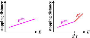
This question can be addressed from first principles in various theoretical limits. One such limit is that of weak coupling, which in principle applies to asymptotically large temperatures and jet energies , for which the relevant running values of are small. In that limit, the stopping distance for a high-energy parton () scales with energy as , up to logarithms.111 A specific weak-coupling calculation of the stopping distance for QCD in the high-energy limit may be found in ref. stop . However, the scaling of this result was implicit in the early pioneering work of refs. BDMPS ; Zakharov on bremsstrahlung and energy loss rates in QCD plasmas. Introducing supersymmetry will not change the conclusion that the stopping distance scales as (up to logarithms) at weak coupling. A contrasting limit of interest occurs when the running values of relevant to jet stopping are all large.222 In a weak-coupling analysis, the two running couplings relevant to jet stopping are, roughly, and , where grows slowly with energy and is the scale of the typical relative momentum between two daughter partons when a high energy parton splits through hard bremsstrahlung or pair production. ( is a scale characteristic of the plasma that parametrizes transverse momentum diffusion of high-energy partons.) A third limiting case of interest, not addressed in this paper, is where is large but is small. See, for example, Liu, Rajagopal, and Wiedemann LRW . This problem is not very tractable from first principles in QCD itself, but, through gauge-gravity duality, progress can be made for QCD-like plasmas with gravity duals, such as super Yang Mills (SYM) theory. For some years, people have considered various ways to study analogs of jet stopping in such plasmas, namely the stopping distance for various types of localized, high-momentum excitations. The exact stopping distance depends on details of exactly how the “jet” is prepared, but universally these studies have found that the maximum possible stopping distance scales with energy as GubserGluon ; HIM ; CheslerQuark ; adsjet ; adsjet2 ; CHR , in contrast to the weak-coupling scaling of . This is an interesting theoretical result because it teaches us that the scaling of jet stopping with energy depends on the strength of the coupling. It remains an open question (which we will not answer here) how starts to move toward as one lowers the coupling, and vice versa.333 See the conclusion of ref. R4 for further discussion of this point.
The stopping distance of high-momentum, localized excitations traveling through the plasma depends on more than just the energy of the excitation. Depending on exactly how one creates the excitation (the “jet”), one may get stopping distances significantly smaller than the maximum . As an example from weak coupling, imagine that we spread out the total energy and momentum of the jet among 10 partons, each having energy , rather than putting it all into a single parton of energy . Each of the 10 partons has lower energy than the single one and so will stop sooner; so the stopping distance for the high-momentum excitation depends on how many high-energy partons we use in the initial state. In the weak-coupling case, the maximum stopping distance corresponds to the particular initial state where all the energy is concentrated into a single initial parton.
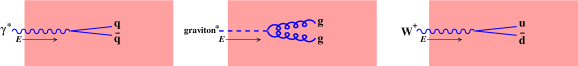
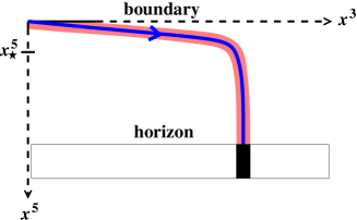
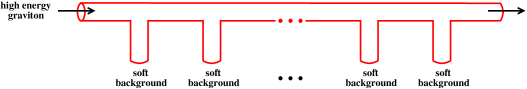
In the strong-coupling case, we cannot speak of individual partons, but the stopping distance again depends on how we prepare the initial high-momentum excitation. In our work adsjet ; adsjet2 ; R4 , we create the initial excitation in a way that is analogous to what you would get if a high-momentum, slightly virtual photon (or graviton or other massless particle) decayed hadronically in the quark-gluon plasma, as depicted in fig. 1. Alternatively, one could consider the decay of a high-momentum on-shell W boson (also depicted). For these methods of creating “jets,” one finds that the maximum possible stopping distance scales as
| (1) |
As we will review later, it turns out that the stopping distance may be made smaller than (1) by varying the virtuality of the virtual photon (or equivalently the mass-squared of the on-shell W boson) HIM ; adsjet2 . The important point is that there is a range of stopping distances for our “jets,” depending on the details of how those excitations are created.
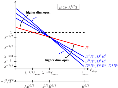
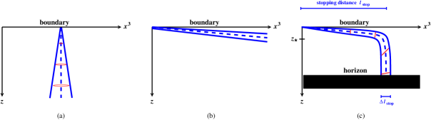
Most top-down studies of jet stopping using gauge-gravity duality have studied the infinite color and infinite coupling limit, and , where is the ’t Hooft coupling. To understand the true high-energy behavior, however, it is important to study the corrections to these limits. As an example, fig. 2 shows two different scenarios one might imagine for the maximum stopping distance for strongly-coupled SYM. One is that grows like at high energy, up to arbitrarily high energies. The other is that it starts growing like at high energy , but then crosses over to some different power-law behavior once exceeds some positive power of times (e.g. in the figure). In the latter case, would not be the true behavior for arbitrarily large and large but finite . But there is no way to tell the difference between these two scenarios if one only has calculations! For this reason, three of us analyzed the parametric size of finite- corrections to jet stopping distances in ref. R4 . We found that the formal expansion in (which corresponds to an expansion in the string parameter on the gravity side) breaks down for some jets and is safe for others, depending on the stopping distance of the jet (and therefore on the virtuality ), as depicted in fig. 3. The stopping distance and virtuality parametrize the horizontal axis in this figure. The vertical axis is a relative measure of the importance of a given correction compared to the result (see ref. R4 for details). The curves are labeled by the sequence of higher-curvature terms in the gravitational dual theory action that correspond, via the AdS/CFT correspondence, to a sequence of corrections in powers of in the 3+1 dimensional SYM theory. Throughout, is taken to be infinite. The result of this study was that, for , corrections to the result are parametrically small for . In particular, corrections to the maximum stopping distance are small. But the interesting case is when jets are created in such a way that
| (2a) | |||
| which is | |||
| (2b) | |||
In this case, the fate of results for the stopping distance was unclear. For , all the corrections are the same size, and so the formal expansion in powers of has broken down. Yet the individual corrections are all small (of relative importance ) for that . From fig. 3, we cannot tell whether the sum of the corrections to will remain small for or whether, instead, the calculation becomes useless there.
The purpose of the present paper is to understand the physics (on the gravity side) of what is going on in the region (2) where the naive expansion in powers of (powers of ) breaks down, and to figure out how to account for the effect of this physics on the jet stopping distance. Note that the interesting window (2a) of stopping distances exists only if the energy is large enough that . By (1), this requires , which we will assume throughout the rest of this paper.
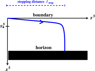
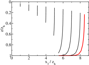
Before outlining what we have done, it will be useful to first explain one other qualitative feature of the calculation. Excitations created in the field theory correspond to excitations created on the boundary of AdS5-Schwarzschild, which then fall towards the black brane over time, such as depicted in fig. 4. The 3-space distance that this excitation travels before falling into the horizon matches the stopping distance of the corresponding excitation in SYM.444 See ref. adsjet2 for a discussion in the context of the present paper, but this correspondence is implicit in the earlier work of refs. GubserGluon ; HIM ; CheslerQuark . For , which includes the region (2) of interest, there is a nice simplification. On the gravity side, the excitation falling in fig. 4 turns out to be a spatially small wavepacket which can be treated in the geometric optics approximation. The wavepacket’s motion is the same (up to parametrically small corrections) as that of a 5-dimensional “particle” traveling in the AdS5-Schwarzschild geometry, and so it follows a geodesic whose trajectory is easily calculated in terms of the 4-momentum of the excitation. (See section III.2 for more detail.)
It will be important for what follows to remember that the AdS/CFT correspondence is really a correspondence between field theory and 10-dimensional string theory. In the strong-coupling limit of the field theory, the general correspondence reduces to one between the field theory and the infrared limit of the string theory, which is a supergravity theory. The quanta of the supergravity fields correspond to string states that are massless in flat 10-dimensional spacetime, such as the graviton. For , the well-known gravitational dual of finite-temperature SYM is Type IIB supergravity in an (AdS5-Schwarzschild) background.
I.2 What we find
The classical wave packet falling in fig. 4 is a localized, classical excitation of the supergravity fields. For the sake of specificity, consider the case where it is an excitation of the background gravitational field. In general, a classical wave is a coherent superposition of the corresponding quanta, and so our high-frequency classical wavepacket is a coherent superposition of high-frequency gravitons. Since our wavepacket behaves like a particle (in the geometric optics approximation appropriate for ), let’s follow just one of these gravitons. So think of the trajectory in fig. 4 as that of a single high-momentum graviton with a localized wave function. As we will discuss later, interactions between the gravitons that make up the wavepacket are very small, and so it is adequate to think about the evolution of individual high-momentum gravitons.
A graviton is really a tiny loop of string whose internal degrees of freedom are in their ground state. Because of the gravitational field from the black brane, this closed string will feel tidal forces as it falls, which will try to stretch the string in some directions and squeeze it in others. As the graviton gets further from the boundary (and so closer to the black brane), the tidal forces will increase, and eventually they will become large enough to excite the internal string degrees of freedom of the graviton. We will argue that it is the excitation of these string degrees of freedom that is responsible for the breakdown of the expansion in fig. 3 in the problem region (2).
We will find that, in the problematic case (2) where , the tidal forces are strong enough to stretch that loop of string to become classically large before the stopping distance is reached. This is why stringy corrections cannot be ignored in that case, explaining the breakdown of the expansion in fig. 3. (In contrast, the tidal forces are not strong enough to excite the graviton’s internal degrees of freedom soon enough when .) Though the resulting classical string loop will be large compared to the size of a graviton, we should ask how its size compares to the stopping distance . We will find that the ratio of (i) the stretched, classical string’s size in the direction of motion to (ii) the stopping distance is parametrically of order
| (3) |
Because of the , this ratio is typically parametrically small for large but finite , and we will argue that the stretching of the graviton into a string (and the accompanying breakdown of the formal expansion in in fig. 3) then has sub-leading impact on results for the stopping distance. But (3) also includes cases where the stretching of the string may play an important role: If one considers a situation where the argument of the logarithm in (3) is exponentially large, then the logarithm can be large enough to compensate for the factor of . We discuss this situation further in our conclusions, where we make contact with folded classical string configurations that were originally used by Gubser et al. GubserGluon to model jet stopping.
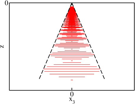
Since the tidal forces stretch a quantum string (the graviton) into a larger classical string, one may wonder whether or not it is possible to do a real, detailed calculation of the transition between the two. Having restricted attention to a single graviton, our problem reduces to following the evolution of a single closed string in the AdS5-Schwarzschild background. In general, it is not known (for all practical purposes) how to quantize a string in an AdS5-Schwarzschild background. But remember that our graviton is localized and so only probes a region of space-time near the geodesic depicted in fig. 4. It is enough to consider only a narrow region of the space-time that lies near a null geodesic, as depicted in fig. 5, and so we may treat the full background metric in an approximation (known as a Penrose limit) that treats displacements from the null geodesic as small. The resulting approximation to the background metric is an example of what is known as a pp-wave background, and it is known how to quantize a string in a pp-wave background. In particular, it will be possible to calculate the probability distribution of the shape of the classical string loop. The methods we use are similar to previous works by other authors on the excitation of string modes in scattering processes and/or in pp-wave backgrounds Veneziano ; PRT ; HS ; GPZS ; dVS .
In the next section, we give a simple, back-of-the-envelope argument that yields the result but is not precise enough to explain the logarithmic factor in (3). Back-of-the-envelope estimates are sometimes enlightening and sometimes frustratingly unconvincing, and the rest of the paper is devoted to a more formal calculation along the lines just described. We set up our notational conventions and review calculations in section III. Next we review in section IV the source of the breakdown of the expansion for , depicted in fig. 3, and use it to motivate why these problems should be overcome by following the quantum evolution of single closed strings in the AdS5-Schwarzschild background. In section V, we take the relevant Penrose limit of the AdS5-Schwarzschild metric, crudely depicted in fig. 5. We are then ready to quantize the string in section VI and solve for the evolution of the graviton into a classical loop of string. We then compute the average size of the resulting classical loops of string, which parametrically gives (3), including the logarithmic factor, for the interesting case . Some readers may wonder how a quantum treatment of the stretching of gravitons can underlie the analysis, given that the gravitational/string dual theory is supposed to be classical in the limit taken in this paper. We discuss this in section VII, where we also give a more detailed justification for treating the gravitons in the wavepacket as independent. In section VIII (supplemented by Appendix B), we then revisit the Penrose limit used in our analysis and verify that it is justified, provided that (3) is small. Finally, we offer our conclusions in section IX.
II A back-of-the-envelope estimate
In this section, we will make a parametric estimate of the amount of tidal stretching of the string compared to the size of the stopping distance . In a later section, we will review the results for how the stopping distance depends on the energy and 4-virtuality of our jet source, but here the only thing we will need to know is that the stopping distance given by following a null geodesic as in fig. 4 is proportional to a power of the slope of that geodesic where it starts, at the boundary. The more downward-directed one starts the trajectory in fig. 4, the less distance it will travel in before reaching the horizon.
Now interpret the trajectory of fig. 4 as a trajectory for the center of mass of a tiny, falling loop of string. Once the string gets far enough from the boundary that the tidal forces dominate over the string tension, then the string tension becomes ignorable, and different pieces of the string will fall independently along their own geodesics, the string stretching accordingly. Imagine plotting two such geodesics, for the two bits of the string loop that are most separated. The separation of those geodesics is a measure of the extent of the tidally-stretched loop of string as it falls towards the horizon. The proper size of the string should start out of order the quantum mechanical size of the graviton, which is roughly set by dimensional analysis in terms of the string tension as
| (4) |
where is the string slope parameter.
Very close to the boundary, the tidal forces due to the black hole are negligible, and the closed loop of string is in its ground state. We can set up our two geodesics above so that, correspondingly, they maintain constant proper separation near the boundary, where the AdS5-Schwarzschild metric approaches a purely AdS5 metric. To see how this works, imagine making a 4-dimensional boost from (i) the plasma rest frame, in which we create an excitation with large 4-momentum and relatively small 4-virtuality , to (ii) the excitation’s initial rest frame, where the 4-momentum is instead . The Lorentz boost factor for this transformation is
| (5) |
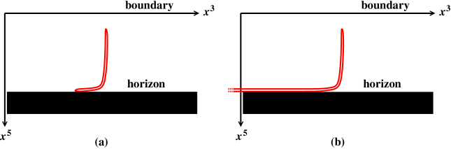
In AdS5, the trajectory in the new frame will drop straight down away from the boundary, as depicted by the dashed line in fig. 6a.
Now consider the graviton as an extended object with proper size . The two straight solid null lines in fig. 6a depict the extent of the graviton in AdS5 in the excitation’s rest frame at early times. In Poincare coordinates for pure AdS5,
| (6) |
null geodesics are straight lines. Here is the radius of the 5-sphere . We parametrize the two solid lines of fig. 6a as
| (7) |
with and . Because of the warp factor in the metric, these two lines are parallel and maintain constant proper separation
| (8) |
as a function of the rest-frame time. Setting this proper separation to be of order the graviton size given by (4) then gives
| (9) |
The AdS/CFT dictionary relates in the string theory with the ’t Hooft coupling of SYM by MAGOO
| (10) |
So
| (11) |
and (7) gives
| (12) |
Now boost back to the original plasma frame using (5) to get the early-time trajectories depicted by solid lines in fig. 6b:
| (13) |
where we have used (5). Then
| (14) |
which represents a small relative variation
| (15) |
in the initial slope of the trajectory. As discussed before, the stopping distance (which requires a calculation in the full AdS5-Schwarzschild metric) covered by a null geodesic is power-law related to this initial slope, and so the difference in how far the two bits of string travel also has the same small size (15) relative to :
| (16) |
This is just our parametric result (3) quoted in the introduction but without the logarithmic factor. The logarithmic factor requires a more detailed analysis.
III Setup
III.1 Notation
In this paper, we will use Greek letters for 4-dimensional space-time indices () and upper-case roman letters for indices that run over all 5 dimensions of AdS5-Schwarzschild (). One form of the metric we use for AdS5-Schwarzschild is
| (17) |
where is the coordinate of the fifth dimension, is the radius of the 5-sphere (which will drop out of final results), and
| (18) |
The boundary is at , and the horizon is at
| (19) |
We will not need to worry about the details of regularizing the location of the boundary in this work.
III.2 Review of calculation
Fig. 1 gave a cartoon picture of how we create our “jets” in the plasma. Readers may find a precise description of the field theory problem in any of the previous papers adsjet ; adsjet2 ; jj ; R4 utilizing this method, but we will not need those details here. Suffice it to say that, in the gravity description, the boundary is perturbed in a localized region of space-time in such a way as to create an excitation with large 4-momentum and a relatively small amount of time-like 4-virtuality . The response of the system is then tracked at late times to see where the excitation comes to a stop.
The supergravity field that is excited depends on the nature of the source for the jet and is the supergravity field dual to the vertex operator in fig. 1. For example, if we study the decay of a slightly off-shell graviton in the 4-dimensional quantum field theory, then the relevant supergravity excitation is in the 5-dimensional gravitational field; if we were to study the decay of a gauge boson weakly coupled to R charge in the 4-dimensional quantum field theory, then the supergravity excitation would be in a corresponding 5-dimensional gauge field; and so forth.
As mentioned in the introduction, there is a nice simplification to the analysis of this problem adsjet2 when . On the gravity side, the wavepacket’s motion is then the same (up to parametrically small corrections) as that of a 5-dimensional “particle” traveling in the AdS5-Schwarzschild geometry, and so it follows a geodesic whose trajectory is easily calculated in terms of the 4-momentum of the excitation. The exact geodesic depends on the mass of the 5-dimensional “particle” and so on the mass of the 5-dimensional supergravity field that we have excited, but this mass (if any) may be ignored in the high energy limit.555 The relevant 5-dimensional supergravity field is the one dual to the operator used to create the “jet” excitation in SYM. The mass of the supergravity field is determined by the conformal dimension of that operator, e.g. for scalar operators Witten , where . We emphasize that is a mass in the 5-dimensional supergravity theory and has nothing to do with “mass” of a jet from the point of view of the 3+1 dimensional SYM quantum field theory.
As a result, attention may be restricted to null geodesics, which are given by
| (20) |
Using the metric (17), the stopping distance is then found to be adsjet2
| (21) |
An important feature of the integral in (21) is that it is dominated by small values of , of order
| (22) |
corresponds to the parametric scale in fig. 4, where the trajectory turns over and beyond which 3-space motion rapidly slows to a stop. The stopping distance is determined by the behavior of the trajectory at .
IV Discussion of expansion
We now want to consider corrections to the results for the stopping distance in the case . First, we take a moment to review the generic story of corrections in the AdS/CFT correspondence, which relates MAGOO
| (23) |
| (24) |
where is the string loop expansion parameter. The string tension sets the mass scale for massive string excitations, and so corresponds to taking the scale for massive string excitations to infinity. For , the strongly-coupled 4-dimensional quantum field theory is therefore dual to the infrared limit of the 10-dimensional string theory, namely supergravity, in the appropriate background. For large but finite , massive string modes are not completely ignorable, and the effective supergravity theory of the massless modes gets corrections, in the form of higher-dimensional terms in its action, from integrating out the effects of the massive modes. Schematically, the effective supergravity Lagrangian becomes666 The precise details of which terms appear independently in (25) and which do not will not matter to our discussion, but Table I of ref. Stieberger gives a nice summary of what’s currently known at tree level (i.e. corresponding to ).
| (25) |
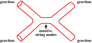
where we have focused just on the gravitational fields for simplicity. represents factors of the Riemann tensor, and we have not shown numerical coefficients or how the indices contract. For , there are no loop effects (), and accounting for the massive string modes in the effective theory is analogous to replacing the effects of the W boson by the Fermi 4-point interaction in electroweak theory. So, for example, the terms in (25) are calculated from string amplitudes for graviton scattering and, crudely speaking, they correspond to processes which involve intermediate massive string states, as depicted schematically in fig. 7. (A more accurate statement would be that they correspond to the full string amplitude for graviton-graviton scattering minus the sum of the , , and -channel graviton exchange diagrams that one would calculate in the supergravity theory.) The terms similarly account for corrections to the 5-point graviton interaction, and so forth.
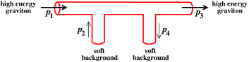
In our application, we are interested in the evolution of a high-energy excitation propagating through the soft AdS5-Schwarzschild background. For simplicity of presentation, we will focus on the case where the excitation is in the 5-dimensional gravitational fields, though our conclusions will not be sensitive to this assumption. A classical gravitational excitation can also be thought of as a coherent configuration of gravitons, and the relevant string scattering amplitudes are those where two of the external lines are the incoming and outgoing high-energy gravitons and the others are the soft background field. So, for a 4-point scattering amplitude such as fig. 7, the relevant kinematic limit is that depicted in fig. 8. With the notation used in that figure, the high-energy limit corresponds to potentially large but small . [Here and throughout we may think of the ’s as 5-dimensional momenta in AdS5-Schwarzschild rather than 10-dimensional momenta in (AdS5-Schwarzschild) because in our problem there is no interesting dynamics associated with the 5-sphere .] As discussed in ref. R4 , the terms in (25) all become equally important in the jet stopping problem when this 5-dimensional becomes large enough at to excite massive string modes in fig. 8. The string mass scale is of order , and this condition
| (26) |
is shown in ref. R4 to be the same, in the context of the jet stopping problem, as the condition
| (27) |
which is the problematic case (2) highlighted in our introduction. In this region, massive string states in the intermediate state in fig. 8 are kinematically accessible and cannot be ignored.
As the high-energy excitation falls from the boundary to the horizon, as in fig. 4, it does not just interact with the background field once or twice but does so over and over again, as depicted in fig. 9. If the massive string states are kinematically accessible as in (26), then they cannot be neglected in any of the internal lines, which means in the effective theory language of (25) that all terms will also become important. This is just what happens at the point in fig. 3, where all the corrections become the same size, corresponding to the threshold . Also, note that if massive string modes are kinematically accessible for intermediate states, then they are also accessible as final states. (In our problem, however, there is never really an ultimate “final” asymptotic state of the excited graviton because the excited graviton falls into the black brane.)
Interaction with a pure AdS5 background does not produce these massive string mode excitations. On a technical level, the interactions really involve the Weyl tensor (the traceless part of the Riemann tensor), which vanishes for AdS5 but not for AdS5-Schwarzschild. So it is only the gravitational effect due to the presence of the black brane that contributes to massive string mode excitation. As a result, the effects of excited string modes are negligible at the boundary and become stronger as one moves away from it (and so closer to the black brane). At some distance from the boundary which we will review later, the gravitational effects of the black brane become strong enough that (26) is satisfied, which is when string modes may first be excited.
From the point of view of an effective theory (25) of gravitons, having all the correction terms become the same size (or worse), seems like an hopeless disaster for the purpose of computations. However, the picture of fig. 9 suggests a different tack. What is happening is that the 10-dimensional gravitons which make up the classical excitation are really tiny (quantum) loops of string which are getting their internal string degrees of freedom excited as they fall in the background gravitational field. Specifically, internal degrees of freedom of a small object are affected by gravitational tidal forces, which try to compress the object in some directions and stretch it in others. In any case, consider the fate of a single graviton as depicted by fig. 9: a high-momentum object moves through a soft background field. Various authors have previously studied applications of the eikonal approximation to string scattering eikonal ; Veneziano . The upshot, as reviewed below, is that fig. 9 may be replaced by the evolution of a single string quantized in the classical background field.
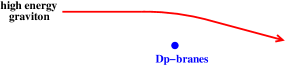
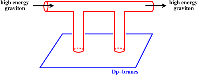
One might simply assert that the right thing to do in the eikonal limit is to quantize a single string in the classical background field, but there is a very nice paper by D’Appollonio, Di Vecchia, Russo, and Veneziano Veneziano that explicitly checks this in a closely related context. As the source of their gravitational field, they take a stack of coincident Dp-branes in otherwise-flat 10-dimensional space-time. They then probe this gravitational field by scattering a high momentum, massless closed string (such as a graviton) from it. The geometry of the situation is depicted in fig. 10, which shows the probe particle moving in two of the asymptotically-flat spatial directions perpendicular to the Dp-branes. The particle is deflected by the gravitational field of the Dp-branes. (If these were D0-branes in 4-dimensional space-time, this could be a picture of a particle deflected by the gravitational field of the Sun.) Their problem is slightly different from our problem in that their particle eventually escapes back to infinity, given the geometry of their setup, but never mind that. They further assume that the impact parameter in fig. 10 is large enough that . This is the assumption that the background field experienced by the particle is soft, its momentum components small compared to the particle’s energy. After discussing the eikonal approximation more generally, they then make the following check. Consider the elastic amplitude for the string loop to interact exactly twice with the Dp-branes as it flies by and to emerge in the same massless state at the end. They perform this calculation in two different ways. One way is to do the full string calculation in the presence of the D-branes, as depicted in fig. 11. The other way is to simply quantize a single string loop in the classical gravitational background caused by the D-branes by taking the Penrose limit of the metric near the string trajectory and quantizing the string in the resulting pp-wave background. Then they calculate to second order in that background. In the eikonal limit, they verify that they get exactly the same result with either method. The calculated probability for the string to remain in its massless state drops rapidly below 1 once the kinematic threshold for exciting internal string modes is exceeded.
With this reassurance, we now turn to taking the Penrose limit and quantizing the string in our own problem.
V The Penrose Limit
We begin by taking the Penrose limit to describe a narrow region around the null geodesic (20), depicted earlier in fig. 5.777 Penrose limits have previously been studied in AdS5-Schwarzschild by Pando Zayas and Sonnenschein LeoPenrose , but the null geodesic studied was different. Their geodesic fell straight toward the horizon in AdS5-Schwarzschild, corresponding to in our problem rather than . Their geodesics also have non-trivial motion on the 5-sphere . In our application, no dynamical evolution of the degrees of freedom takes place: the internal modes of the string stay in their ground state, and the zero modes of the string simply remain in a quantum state given by the harmonic of the supergravity field of interest. Equivalently, our worldsheet vacuum has conserved charges that are equal to those of the harmonic of the supergravity field of interest. For an overview of taking Penrose limits, see Refs. Blau ; BlauLecture ; BlauFermi .
The null geodesic (20) can be written as
| (28a) | |||
| where is an affine parameter for the geodesic determined by888 This should not be confused with the coordinate used in earlier work by some of the authors adsjet ; adsjet2 . | |||
| (28b) | |||
which can be integrated to give as a function of . The normalization of is just convention, and the canceling factors of in (28) have just been chosen to give dimensions of length. In the metric (17), is given by
| (29) |
which is linearly divergent as . Our convention will be to define as running from at the boundary to at the black brane singularity, and so
| (30) |
The important thing to remember in what follows is that late times correspond to small negative values of (which we will later also call ). Also, though it will be convenient to have defined to be at the singularity , all of the physics we discuss will only depend on what happens outside of the horizon, .
We’ll refer to our reference geodesic as , which we choose to start at the origin on the boundary. Now measure 4-positions in AdS5-Schwarzschild relative to this geodesic by defining
| (31) |
Take to be in the direction. Changing coordinates from and to and
| (32) |
puts the AdS5-Schwarzschild metric (17) into the form
| (33) |
where is now implicitly a function of . The Penrose limit consists of keeping only the terms in the metric that would dominate after a scaling of coordinates
| (34) |
for very large . This is analogous to making what would be a very large boost (, ) in flat space, and so looking at physics close to the light cone, followed by rescaling all coordinates by a factor of . For (33), the resulting limit is
| (35) |
which is a particular example of a pp-wave metric. When we are done with our analysis, we will go back and check that this approximation is justified. The coordinates used in (35) are known as Rosen coordinates.
The metric (35) has the schematic form
| (36) |
It is useful to normalize the last term by switching to Brinkmann coordinates
| (37) |
and
| (38) |
to give
| (39) |
In our case, using (29) to rewrite
| (40) |
the metric in Brinkmann coordinates is
| (41) |
with
| (42a) | |||
| (42b) | |||
| (42c) |
Here, primes denote derivatives with respect to , and is implicitly a function of , determined by inverting (30). The metric (41) would be flat if not for the , which arise from tidal forces. Note that these tidal terms vanish for null geodesics in pure AdS (, or equivalently ), in agreement with general arguments that the Penrose limit of AdS is flat Minkowski space Blau . They also vanish in AdS5-Schwarzschild if (i.e. if the excitation fell straight down in the direction as a function of time ).
VI Quantizing our falling string loop
VI.1 Overview
We may now follow other authors to quantize a string in a pp-wave background Veneziano ; PRT ; HS ; GPZS ; dVS . The bosonic sector is described by a -model in the pp-wave background metric:
| (43) |
where is the world-sheet metric and are the world-sheet fields corresponding to the coordinates. For the pp-wave space-time metric (41), this takes the form
| (44) |
where is the Minkowski string action. Identifying world-sheet time with the affine parameter for the pp-wave space-time metric (41) then gives a constraint equation for and gives the light-cone gauge Lagrangian
| (45) |
for the , where and and
| (46) |
(We have suppressed the fields corresponding to coordinates because they will play no role in our discussion.) Note that we have chosen a convention where has units of time and is dimensionless.999 A more conventional normalization might be to define a dimensionless as instead of our . One may convert to this convention by everywhere replacing our by . In our convention, the world-sheet metric is
Each mode of the string is a time-dependent harmonic oscillator problem with classical frequency . The and modes are tidally compressed as the string moves away from the boundary since is negative in (42b), so that the curvature of the harmonic oscillator potential increases with time . In contrast, the oscillators are tidally stretched, since is positive in (42c). We will focus on these degrees of freedom and so will focus on
| (47) |
When the string gets far enough from the boundary (i.e. at late enough times ), the term in (47) becomes dominant and oscillators become unstable. Physically, this is when tidal forces come to dominate over string tension. Using (42c), this instability occurs when , where
| (48) |
The instability for the center-of-mass mode is not particularly interesting: it has nothing to do with exciting internal degrees of freedom of the string and just reflects the slight spread of the falling wavepacket in fig. 4 due to curvature effects. That is, it reflects physics already incorporated in earlier work adsjet2 on our jet stopping problem and has nothing to do with gravitons being tidally stretched into classical strings. So, in what follows, we will focus on the modes, and the first tidal instability kicks in at .
Recall that , defined in (22), characterizes the scale where the motion of the bulk excitation in fig. 4 is coming to a stop (no significant motion for ). How does the instability scale above compare to ? Using (21) and (1), the ratio is
| (49) |
So the tidal instability kicks in before the stopping distance is reached () precisely when we are in the interesting regime (2) identified in earlier work as the case where stringy corrections become important. This is the case we focus on. Correspondingly, the modes which become tidally unstable for are with
| (50) |
Although the instability develops at , we will see later that the modes do not have time to stretch significantly until . This fact is suggested by the geodesic picture in fig. 6: For , the impact of the black hole on the evolution in fig. 6c is negligible, and so the evolution at those times is well approximated by the pure AdS case of figs. 6a and b, for which the proper size of the string remains constant.
Once a given mode becomes unstable, the quantum mechanics of that mode will be somewhat analogous to a standard quantum mechanics thought experiment: What is the longest time that an idealized pencil can be balanced on its tip before it falls? Because of the uncertainty principle, the pencil cannot be started simultaneously at rest and perfectly vertical, and so it must fall. The pencil might be started in a Gaussian wavepacket chosen to maximize the average fall time. But it is clear that, once the top of the pencil has fallen a macroscopic distance, classical mechanics will suffice to describe its subsequent motion: at that time, its position and momentum may, to excellent approximation, be considered as simultaneously well defined. For late enough times , the pencil’s motion for is approximately classical, with the only effect of its initial wave packet at being to determine a classical probability distribution for the pencil end’s position at . The corresponding momentum at is given (to excellent approximation) by the momentum the pencil would have picked up falling classically to that position from vertical.
In our problem, we will see that, for the string modes of interest, the analogous transformation from a quantum description to a probability distribution for classical configurations occurs when .
VI.2 Solution of the time-dependent harmonic oscillators
VI.2.1 Basics
The distinction between (the difference between and the reference geodesic) and does not affect the modes that are our focus. Similarly for the normalized coordinates . So we will make our notation a little less cumbersome and henceforth write as simply (for ).
Each of the real degrees of freedom and in (45) have a harmonic oscillator Lagrangian of the form
| (51) |
with the translation and . The squared frequency starts at a non-zero value and then changes with time . The quantum mechanical solution to such time-dependent harmonic oscillator problems has a long history. Useful explicit formulas for wave functions may be found in ref. KimLee , with applications to strings in pp-wave backgrounds in refs. PRT ; GPZS .101010 The case (53) of interest to us corresponds to the ground state cases ( or ) of refs. PRT ; GPZS ; KimLee , and our here corresponds to their , , or respectively. However, there are various normalization issues in the formulas in all of these references, which all differ from us and from each other by overall powers of our in their expressions for the final wave function, though most differences are probably typographic errors. is just a time-dependent but -independent complex phase, and so such differences will not matter for the evaluation of an expectation value in one of these states. But, if one wants explicit solutions to the time-dependent Schrödinger equation, then the phase needs to be correct. A simple test of any such result is to consider the case where is constant and verify that reproduces the correct time dependence . Accordingly, the in (5.37) of ref. PRT should be , the in (2.16) [(2.15) in the preprint] of ref. GPZS should be , and the in (3.9) of ref. KimLee should be if one wants to keep track of the overall time-dependent phases and have results that solve the Schrödinger equation. Note added: Formulas with the correct phase may be found in ref. KimPage . In our case, the harmonic oscillators all start in their ground state (the string state describing a graviton) at early times () and so start with Gaussian wave functions. For a time-dependent harmonic oscillator that starts as a Gaussian at some time , one may check that the Schrödinger equation
| (52) |
is solved by
| (53) |
where the complex-valued function satisfies the classical equation of motion
| (54) |
with initial conditions
| (55) |
In our case, where we start in the early-time ground state, that’s
| (56) |
with .
It will be useful to have an expression for the corresponding probability distribution for . From (53), this is just a Gaussian distribution
| (57) |
with width
| (58) |
But is a Wronskian of the two solutions and of (54) and so is time-independent and may be evaluated at using (56), giving
| (59) |
Using (47), corresponds to in our application.
Our remaining task is to solve the classical equation of motion (54) for . For the case of interest , using (22), (40), (42c), (47), and , the equation may be put into the form
| (60a) | ||||
| (60b) | ||||
where
| (61) | ||||
| (62) | ||||
| (63) |
In these variables, the initial conditions (56) on are
| (64) |
Note from (1) and (21) that, parametrically,
| (65) |
and so the smallness of is a specific measure of how far we are into the interesting regime (2) of . The modes of interest to us correspond to .
Using the above equations, one may now check our earlier claim that the string does not stretch significantly in proper size at early times ().111111 The argument is a distraction and so relegated to this footnote. For (), one may ignore the term in (60a) and treat as small. In this case the two independent solutions are approximately and , with . (See Appendix B.2 for a more general discussion of solutions, for which the ones here are the small limit.) To match to the oscillating solution for for determined by (64), the superposition of and for must be , where denotes coefficients with magnitude of order 1. We then see that is approximately constant over the time period . But we are more interested in what the string does at late times, on which we now focus.
VI.2.2 Late-time behavior
For (which is ), the equation (60b) gives
| (66) |
remembering that our convention is that is negative and that . Note from (66) that is very small at the horizon , where . Throughout this paper we assume that and so .
Plugging (66) into the equation (60a) yields late-time () solutions and . The dominant solution will be
| (67) |
Though is a complex-valued function whose purpose is to track the evolution of the wavepacket, exactly the same arguments as above give that a classical trajectory would have late-time behavior . That means that , and so and both become large at late times, justifying a classical description at late times.121212 For example, at late times the exponential in the wavepacket (53) becomes , where . The WKB condition is satisfied as for . We will see shortly that the proportionality constant in (67) is of order 1 for the modes of interest. If one keeps track parametrically of all the proportionality constants in the exponential , one finds more specifically that the WKB condition is satisfied when (i.e. ). The classical relation between the two is determined by to be
| (68) |
We may extract the proportionality constant in the late-time behavior (67) by solving (60) numerically with initial conditions (64) for , matching the late time behavior of the numerical solution to (67), and repeating the calculation for earlier and earlier values of in order to take the limit. Our result is that the late-time behavior is
| (69) |
with given by fig. 12.131313 For numerical work, it is mildly convenient to eliminate and express all of the relevant equations solely in terms of , giving and (with ) and (as ). We show in Appendix A that the limiting behavior for large is
| (70a) | |||
| shown as a dashed curve in the figure. In the opposite limit of , our numerical results approach a constant | |||
| (70b) | |||
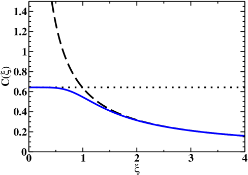
From (47), (59) and (69), and remembering that the analogs of are and , the late time probability distribution of mode amplitudes is given by a Gaussian with width
| (71) |
Using (66), that may be rewritten as
| (72) |
As in (68), the corresponding momenta in this classical regime are related to the mode amplitudes by
| (73) |
Using (35) and (37), the conversion between the normalized coordinate and the displacement from the reference geodesic in Poincare coordinates is
| (74) |
which is
| (75) |
So, from (72), the amplitudes of the stretched modes in the Poincare coordinate system are
| (76) |
for fixed (and so fixed ) in the classical regime. Using (21) and (22), this may be written as
| (77) |
for .
Note that fixed- (i.e. fixed-) slices of the string worldsheet look different than fixed- slices of the string worldsheet, which is why our depiction of the string at various times in fig. 6c were not horizontal.
VI.3 The size of the string at late times
Parametrically, the average size (77) of each stretched mode in Poincare coordinates is just the that we found in our back-of-the-envelope argument in section II. But we should now look at what happens if we sum up all the modes to get the total average size of the string. A convenient measure of the size scale of the string is the average rms deviation from the center of the string,
| (78) |
where overlines indicate averaging over the string worldsheet position and the angle brackets indicate averaging over the late-time classical probability distribution for each mode amplitude. This is given by
| (79) |
is just the square of what we called in (77). Combining the limiting forms (70) with (77), and recalling from (63) that ,
| (80) |
where is given by (70b). The sum in (79) is therefore convergent at large (more on that in a moment) and is dominated by a logarithm coming from up to . At leading order in inverse powers of that logarithm,
| (81) |
Using (50), this may be rewritten as141414 A comment on randomness: , determined by (80), is the width of a Gaussian distribution for that is centered on . In contrast, at leading log order, the -averaged extent of the late-time string is always given by the of (82). That’s because, when the logarithm is large, the calculation of the logarithm in (82) involves a sum over a large number of modes, all contributing to the coefficient of the leading log, and so the probability distribution of is narrowly peaked about its probabilistic average by the central limit theorem. The mode by itself is a substantial piece of the first correction beyond leading-log order, and so randomness will enter if one moves beyond a leading-log analysis of .
| (82) |
where a parametric expression for the argument of the logarithm is adequate if we are only keeping track of the logarithmic term.
Ignoring the numerical constant in front, (82) is the parametric result (3) that we presented in the introduction. One could go on to evaluate the non-logarithmic corrections to (82), but (82) is good enough for our present purposes. We are mostly interested in the parametric size of the answer, so that we can determine whether the extent of the string in remains small compared to the stopping distance in the case of large but finite .
Qualitatively, what is the origin of the logarithmic factor in (81) and (82)? Imagine doing the same calculation of for the graviton instead of for the stretched, classical string. In the ground state, all the modes have an rms size proportional to and so the sum is log divergent in the ultraviolet. This does not mean, however, that the energy or momentum carried by the graviton is smeared over infinite spatial distances:151515 For some discussion of the unobservability of the UV log divergence and and how the “size” of a low-mass string excitation should be interpreted, see refs. size . in the string’s ground state, the bosonic mode contributions to energy and momentum are canceled by the fermionic mode contributions, which we have ignored in our analysis. Only the bosonic mode amplitudes, however, can become “big” due to tidal stretching, and it is the modes whose amplitudes have grown big that we consider when we make the classical approximation at late times. Our expression (80) is only valid until gets so large that the bosonic mode has not been significantly excited (, and so when ). For yet larger the modes will be in their ground state and the canceling contribution of fermionic modes to physical quantities of interest will come into play. The contribution of such high modes is sub-leading and is simply discarded when we approximate the string as a classical string at late times. In the resulting treatment of the classical string, there is no ambiguity in what the size of the string means, as highlighted by the convergence of the sum of (80).161616 We point out in passing that this is not an obscure issue specific to relativistic strings. If one quantizes small transverse vibrations of an idealized violin string , the same divergence arises in the calculation of the mean-square displacement of the string. But, if you took a snapshot in time of an actual vibrating violin string (with classically large amplitude), you would not have any real-world confusion about what the mean-square displacement of that string meant. You would only get confused if you perversely chose to resolve the (idealized) violin string on such small distance scales that you could see the quantum uncertainty of very high modes that had not been excited, and for such measurements the classical description of the violin string would be inadequate. If you’re not interested in such high resolution, then the classical result for the average displacement is an excellent approximation and is physically meaningful information.
The upshot is that the logarithm in (81) arises because of (i) the logarithmic UV divergence associated with the bosonic modes in the ground state, combined with (ii) the fact that the bosonic mode amplitudes with all grow by an equal large factor from tidal stretching (and no longer cancel against fermionic modes in their physical consequences), while those with do not grow significantly in comparison.
VII Discussion of the single graviton approximation
We have followed the evolution of a single graviton as it is stretched into a classical string loop. We will now take a moment to discuss in more detail the premise that we may follow a single graviton.
First, a single high-momentum string loop might split into two, but such splitting is suppressed and so may be ignored in the limit that we take in this paper.
The same argument might be given against the possibility of two gravitons merging if not for the fact that the localized gravitational wavepacket describing our excitation in the bulk is classical, which means it contains a correspondingly large number of gravitons. We need a different argument for why interactions between the gravitons that make up the classical wavepacket may be ignored. For this, we need to review in slightly more detail the formalism of refs. adsjet ; adsjet2 for creating the excitation in the first place. In that formalism, the initial photon or W boson or whatever of fig. 1 is replaced by a localized, external classical field. Specifically, we add a source term to the Lagrangian,
| (83) |
where is an arbitrarily small source amplitude, is a source operator (corresponding to the vertex in fig. 1),
| (84) |
is the large 4-momentum of the desired excitation, and is a slowly varying envelope function that localizes the source near the origin in both and time. The amplitude is chosen to be small so that we can treat the external source as a small perturbation to the strongly-interacting gauge theory, so that the source will never create more than one jet with energy at a time. On an event-by-event basis, the source will usually do nothing at all, but on rare occasions (), it will create an excitation with energy . For small enough , it will essentially never create excitations with energies , , etc. adsjet2 . But taking small also means that the bulk excitation created by the source on the boundary can be treated in linear response: the self-interactions of the bulk excitation with itself are ignorable. For this reason, we may ignore interactions between the gravitons (or other type of particles) that make up the bulk excitation.
Some readers may wonder how we can focus on gravitons, which are quantum mechanical objects, when the dual theory for is supposed to be a classical theory. As an analogy, consider a classical electromagnetic wave with polarization . If we choose to, we may think of this classical wave as a coherent superposition of photons which are in the quantum state , where and are states corresponding to polarization in the and directions. Now measure the polarization by putting the wave through a linear polarizer oriented in the direction. As we all know, we may view this classically as picking out the component of the wave, or alternatively we may view it in terms of photons as saying that each photon has probability of being -polarized. A discussion of classical physics in one description is equivalent to a quantum-mechanical discussion of probabilities for the behavior of individual quanta in the other description.
The same reasoning applies to our description of the classical bulk wavepacket in terms of individual gravitons. An important conceptual lesson from this is that our wavepacket is not a single graviton that evolves into a single classical string loop with probability distribution given by a Gaussian with size (82) for each mode . Instead, the wavepacket is a large number of gravitons that independently evolve into a large number of classical string loops that independently have that probability distribution. Following the analogy with photon polarizations further, one could presumably replace the quantum description involving probability amplitudes for the degrees of freedom of individual string loops by a classical description in terms of a classical string field theory, promoting the Schrödinger wave functional for a single string to a classical wave functional that could be used to describe all the physics discussed in this paper. We have not pursued this latter approach because we thought that the description in terms of gravitons was simpler, more intuitive, and more directly related to the previous literature on tidal excitation.
VIII Checking the Penrose limit
Now that we have our final answer (82) for the size of the classical string that is produced by stretching, we should go back and verify that the string is not so big, or so far away from the reference geodesic, that the Penrose limit taken in section V breaks down. We need to check that the and terms in the AdS5-Schwarzschild metric (33), which were dropped in the Penrose limit, are parametrically small compared to the term,
| (85) |
for the string motions that we have found. Dividing both sides by and using , we may rewrite these conditions as
| (86) |
We check these conditions on the string motion in appendix B, where we find that the condition on is the strongest and requires
| (87) |
in order for our earlier analysis to be valid. Using our result (81), this condition may be written as
| (88) |
That is, the Penrose limit only breaks down if one considers the extreme case (to be discussed in a moment) where the string becomes as large as the stopping distance itself.
IX Conclusion
In our scheme for creating “jets,” we have seen different behaviors in the dual theory depending on the virtuality (and so the stopping distance) of the jet. For , the gravitons (or other massless string modes) composing the excitation in the gravity description remain gravitons until after the excitation has stopped moving in the direction, and there is no difficulty in using the supergravity approximation for the calculation. For , each graviton is instead stretched into a classical string loop. However, provided that
| (89) |
the size of that string remains small compared to the stopping distance . The string remains close to its reference geodesic, and so corrections to the description of the jet stopping are parametrically small (if one only attempts to resolve details on size scales large compared to the size of the string). However, if instead
| (90) |
then the string loop will stretch out to be parametrically as large as the stopping distance itself. Our quantum analysis of the string breaks down in this case (because of the failure of the Penrose limit), but we can see what happens qualitatively by tracking what happens to the results as we increase the logarithm towards .
In particular, a nice way to visualize what happens is to follow the classical evolution of a closed string that initially starts with a proper size of order , which is roughly the initial rms size from the modes which become classically excited. Increasing the logarithm towards is equivalent to increasing towards . Fig. 13 compares examples of such evolution for the cases (a) and (b) . (More details of exactly how we initialized our classical string may be found in appendix C.) The interesting feature of fig. 13b is that, at late times, the string looks like the original picture advocated by Gubser et al. GubserGluon of gluon jets as dual to the evolution of a trailing, folded classical string falling in AdS5-Schwarzschild. Our string is a folded closed string, as depicted in the cartoon of fig. 14a, whereas the one studied by Gubser et al. was a folded infinite open string, as depicted by fig. 14b.171717 More precisely, Gubser et al. first considered a folded open string that stretched out from beyond the horizon, as in fig. 1 of ref. GubserGluon . But in actual calculations, they focused on the trailing infinite folded string, as in fig. 2 of that reference. However, the left end of the string in these figures, which is very close to the horizon, does not play a significant role in the effect on the boundary theory, and so the physics of these two situations is approximately the same.

Historically, the original motivation of our own method for posing “jet” stopping problems adsjet , outlined in the introduction to this paper and motivated by fig. 1, was to give a precise field theory problem in SYM that could be solved, beginning to end, using gauge-gravity duality. It has not previously been know how to precisely set up a problem in SYM that corresponds to earlier studies of jets GubserGluon ; HIM ; CheslerQuark that made use of classical strings in the gravity description. It is interesting to now make contact between our approach and Gubser et al.’s classical string approach, in the particular limit (90), which can be roughly rewritten as
| (91) |
where the is thrown in to emphasize that we’ve always been assuming and so throughout, and where means “of order.” Alternatively, in terms of the virtuality of the source of our “jet,” (91) is
| (92) |
This window of stopping lengths only appears once the jet energy is large enough that
| (93) |
Even though there is a region of overlap (91) of our results with strings that look similar to those of Gubser et al., there are still important differences once we get out of this range. Gubser et al. found a maximum stopping distance of order , as do other methods that also model excitations with semi-infinite classical strings in the gravity dual CheslerQuark . In contrast, the types of excitations that we create, through processes like fig. 1, have a parametrically larger maximum stopping distance of order .
In this paper, we have studied the case of large but finite , but we have kept . It is important to mention, following Gubser et al. GubserGluon , that the case of finite may be qualitatively different. For finite , the folded classical string may break, creating many string loops. It would be interesting to understand whether or not such breaking would impact the description of jet stopping in SYM.
Our basic argument in this paper has been that the breakdown of the expansion seen in the earlier supergravity calculation of ref. R4 is explained by the tidal stretching of gravitons into classical string loops. Logically, however, to show that tidal stretching was the only source of difficulty, we should now do a systematic analysis of sub-leading corrections to the string evolution that we have presented here and show that those corrections are indeed parametrically small. We expect that they will be, but we leave that for someone to study another day.
Finally, we mention that an alternative to our method for creating “jets” is to produce gluon jets as synchrotron radiation from heavy quarks that are forced into circular motion. The corresponding jet stopping problem has been investigated for strongly-coupled SYM by Chesler, Ho, and Rajagopal CHR . We suspect that problems similar to those treated here could be set up in that context as well, with appropriate choices of the heavy quark velocity and synchrotron radius for a given temperature . It would be interesting to investigate.
Acknowledgements.
This work was supported, in part, by the U.S. Department of Energy under Grant No. DE-SC0007984.Appendix A Large behavior of
Appendix B Checking the Penrose limit: details
In this appendix, we will check whether the evolution of our strings satisfy the conditions (86) required for taking the Penrose limit. It is illuminating to do this in two different ways. First, we will make a rough argument based on following divergent geodesics, similar to the style of argument that we used in section II. Then we will give alternative (but physically equivalent) arguments based on string-based results and formulas.
B.1 Tracking diverging geodesics
As in section (II), let us characterize the string by following null geodesics that roughly trace different bits of string and which deviate slightly from our reference geodesic. As we’ll discuss again later, this approximation amounts to ignoring the tension in the string. From the null geodesic formula (20) and the metric (17), the coordinate for such geodesics is given by
| (97) |
where
| (98) |
Remembering that is the deviation relative to the reference geodesic, we have
| (99) |
Expand to first order in :
| (100) |
Then using (40) (and defining with respect to the reference geodesic ),
| (101) |
Since , the combination (101) is largest for , and the condition in (86) requires
| (102) |
for the Penrose limit. Use (21) to relate this to the stopping distance:
| (103) |
so that
| (104) |
Combining (102) and (104) gives the condition
| (105) |
quoted in (88).
Now turn to the condition on in (86). The definition (32) of gives
| (106) |
and so we need a formula for . The analog of (97) is
| (107) |
with expansion
| (108) |
Combining (100), (106), and (108), gives . We therefore have to go back and make our expansions to second-order in . The result is
| (109) |
and so
| (110) |
The corresponding condition on in (86) is then
| (111) |
The first condition is strongest for and the second for , giving
| (112) |
Using (104), the condition involving becomes
| (113) |
Since , this is weaker than the previous condition (105).
Now turn to the other condition, in (112). To estimate , return to the arguments of section II, but now, in the rest frame, include an initial proper displacement of the two geodesics in of the same parametric size as the initial proper displacement in . Following through the argument, one finds
| (114) |
with . Then
| (115) |
and
| (116) |
so that
| (117) |
So, using (104),
| (118) |
The condition is therefore the same as the previous condition (113) and so is also weaker than (105).
B.2 String-based formulas
Another way to get to the same result is to start from formulas based on our string analysis in section VI. We will also need the constraint equation for generated by (44) in gauge, which is
| (119) |
Using the definition of (38) of , the corresponding constraint for is
| (120) |
where is the notation introduced in eq. (36) with
| (121) |
The relationship (37) between and is
| (122) |
Alternatively, (120) is just the constraint equation that one would derive in Rosen coordinates (35).
Here and throughout, we will take results derived in the Penrose limit but then use them to check, after the fact, whether the Penrose limit was valid. We will focus on the evolution of the string modes after they become unstable (). The string equation of motion from the Lagrangian (45) is
| (123) |
where . At late times , the tidal terms dominate over the string tension terms , and the equation of motion becomes
| (124) |
which it is convenient to rewrite as
| (125) |
Two independent solutions for in the tensionless approximation (125) are
| (126) |
We will take and to be normalized to be at . The late-time ( string solutions will then be given by some probabilistic superposition
| (127) |
where and are of order the size scale of the proper size of the ground state of the -th mode, which characterizes the string for .
From (40) or (60b), the relationship between and is
| (128) |
Given the expressions (121) for , the resulting behavior of the solution (126) is then
| (129) | ||||
| (130) | ||||
| (131) | ||||
| (132) |
Note that dominates over for . For , we have , and this behavior corresponds to the dominant late-time behavior discussed in section VI.2.2. At late times, differs from a multiple of by corrections of absolute size of order , which is the sub-leading late-time solution discussed in the main text just before (67). A simple way to see this is to rewrite the definition of in (126) as
| (133) |
where the first term is proportional to and the second is (at late times) the sub-leading solution. Similarly, at late times (), differs from a multiple of by sub-leading corrections of order .
B.2.1 Condition on
Now let us investigate the Penrose limit condition (86) on , which can be rewritten as
| (134) |
The solutions do not give any contribution to the derivative above, and so
| (135) |
The condition (134) has to be satisfied for every point on the string. But we can get a sufficient parametric condition by taking the rms average over the modes which are excited:
| (136) |
which then gives
| (137) |
This condition is strongest for and then gives the condition (87) quoted in the main text.
B.2.2 Condition on
Now turn to the condition on . The first term in the constraint formula (120), which is what remains if one ignores the tension terms in that equation, simply reproduce the conditions (111) found in the earlier analysis based on diverging geodesics. To see this, consider the contribution of the first term in (120) to the constraint in (86):
| (140) |
Using (121) and (135), the contribution from mode to the left-hand side of (140) is of order
| (141) |
Summing over the excited modes gives
| (142) |
This is the same as the second condition in (111), with the identification (139) noted before. Similarly, using (121) and (126),
| (143) |
generates
| (144) |
which is the same as the first condition in (111), using the identifications of (118) and (139).
Appendix C Simulation details for fig. 13
Before we explain the initial conditions used to simulate the string evolution in fig. 13, we will take a short detour and explain how to generate a string evolution as depicted in fig. 6a.
First, let us notice that near the boundary, the metric is approximately AdS. So the string evolves at very early times in a geometry which is AdS. Moreover, in the rest frame of the string considered in fig. 6a, if the string has a sufficiently large energy, the string excitations probe a geometry which is the Penrose limit of an in-falling massless excitation in AdS. In other words, these excitations probe flat space. To show this explicitly, we start by expanding around the null geodesic . Defining, as in equations (30–32), , yields
| (145) |
Taking the Penrose limit by scaling the coordinates as in (34) brings the metric into the Rosen form
| (146) |
which is just (35) with (i.e. ). While this is not immediately recognizable as a flat space metric, a change of coordinates to bring the metric into Brinkmann form, , yields
| (147) |
which is the limit of (41). In this geometry we consider the evolution of an initial string configuration with the string shrunk to a point and with , , , where we have defined and by and . The other string coordinates remain zero throughout this section. Since the string is point-like at the initial time, the stress-tensor constraint is trivially satisfied, and the second stress tensor constraint was used to solve for the initial condition on . If we choose and such that , the string has an approximate analytic solution of the form , , , or, in the Brinkmann coordinates, , , .
Next we switch to Rosen coordinates, and we require that the string is again point-like at the initial time : , and , where we introduced a boundary regulator . In order to satisfy this set of initial conditions we only have to perform a shift in in the previous Brinkmann solution, and use the mapping from Brinkmann to Rosen coordinates: , , . This is a solution which oscillates, as depicted in fig. 15 for small . The envelope of these oscillations grows linearly with and roughly corresponds to fig. 6a.
The next step is to perform a very large boost along starting from the rest frame we have been discussing so far. This will give us the appropriate initial conditions used to generate fig. 13a. Again, the string starts as a point-like object very close to the boundary: , , . We take . The initial (worldsheet) time derivatives have the following expressions: , , , where . Here is the energy of the boosted string and is the momentum along the direction in the appropriate units.
Earlier in this appendix, we discussed Penrose limits of AdS in order to motivate our choice of initial conditions. However, we now simulate the evolution of our classical string from these initial conditions in the full AdS5-Schwarzschild geometry, with no such approximation, to obtain fig. 13a. In order to generate a string evolution to sufficiently late times, we followed CheslerQuark ; Herzog and introduced an appropriate stretching function ,
| (148) |
with , , . Then redefine the worldsheet time so that the worldsheet metric is
| (149) |
The numerical evolution of the classical string was carried out using Mathematica.
Lastly, to generate fig. 13b, the initial conditions were modified as follows. The string begins its evolution once more as a point-like object close to the boundary , . But the initial time derivatives are now , and, as before, the remaining derivative is obtained from the constraint .
The main difference between the two initial conditions is that we have increased the small parameter, which is a placeholder for from 0.02 in the previous numerical simulation to 0.6 here. [As a side comment, this parameter cannot be increased to arbitrarily large values or else the argument of the square root in becomes negative.] The stretching function used here is of the same form as in (148), but with different exponents . This string quickly stretches in . Once one of the folding points reaches the horizon, it remains frozen at that particular value of . The net result is that we have now generated a string which is folded back, with one folding point at the horizon and trailing behind the rest of the string, while the other folding point is still close to the boundary. This string is moving with some momentum in the direction.
References
- (1) P. B. Arnold, S. Cantrell and W. Xiao, “Stopping distance for high energy jets in weakly-coupled quark-gluon plasmas,” Phys. Rev. D 81, 045017 (2010) [arXiv:0912.3862 [hep-ph]].
- (2) R. Baier, Y. L. Dokshitzer, A. H. Mueller, S. Peigné and D. Schiff, “The Landau-Pomeranchuk-Migdal effect in QED,” Nucl. Phys. B 478, 577 (1996) [arXiv:hep-ph/9604327]; “Radiative energy loss of high energy quarks and gluons in a finite-volume quark-gluon plasma,” Nucl. Phys. B 483, 291 (1997) [arXiv:hep-ph/9607355]; “Radiative energy loss and -broadening of high energy partons in nuclei,” Nucl. Phys. B 484, 265 (1997) [arXiv:hep-ph/9608322].
- (3) B. G. Zakharov, “Fully quantum treatment of the Landau-Pomeranchuk-Migdal effect in QED and QCD,” JETP Lett. 63, 952 (1996) [arXiv:hep-ph/9607440]; “Radiative energy loss of high energy quarks in finite-size nuclear matter and quark-gluon plasma,” JETP Lett. 65, 615 (1997) [arXiv:hep-ph/9704255].
- (4) H. Liu, K. Rajagopal, U. A. Wiedemann, “Calculating the jet quenching parameter from AdS/CFT,” Phys. Rev. Lett. 97, 182301 (2006) [hep-ph/0605178].
- (5) S. S. Gubser, D. R. Gulotta, S. S. Pufu and F. D. Rocha, “Gluon energy loss in the gauge-string duality,” JHEP 0810, 052 (2008) [arXiv:0803.1470 [hep-th]].
- (6) Y. Hatta, E. Iancu and A. H. Mueller, “Jet evolution in the SYM plasma at strong coupling,” JHEP 0805, 037 (2008) [arXiv:0803.2481 [hep-th]].
- (7) P. M. Chesler, K. Jensen, A. Karch and L. G. Yaffe, “Light quark energy loss in strongly-coupled supersymmetric Yang-Mills plasma,” Phys. Rev. D 79, 125015 (2009) [arXiv:0810.1985 [hep-th]].
- (8) P. Arnold, D. Vaman, “Jet quenching in hot strongly coupled gauge theories revisited: 3-point correlators with gauge-gravity duality,” JHEP 1010, 099 (2010) [arXiv:1008.4023 [hep-th]].
- (9) P. Arnold and D. Vaman, “Jet quenching in hot strongly coupled gauge theories simplified,” JHEP 1104, 027 (2011) [arXiv:1101.2689 [hep-th]].
- (10) P. M. Chesler, Y. -Y. Ho and K. Rajagopal, “Shining a Gluon Beam Through Quark-Gluon Plasma,” arXiv:1111.1691 [hep-th].
- (11) P. Arnold, P. Szepietowski and D. Vaman, “Coupling dependence of jet quenching in hot strongly-coupled gauge theories,” JHEP 1207, 024 (2012) [arXiv:1203.6658 [hep-th]].
- (12) G. D’Appollonio, P. Di Vecchia, R. Russo and G. Veneziano, “High-energy string-brane scattering: Leading eikonal and beyond,” JHEP 1011, 100 (2010) [arXiv:1008.4773 [hep-th]].
- (13) G. Papadopoulos, J. G. Russo and A. A. Tseytlin, “Solvable model of strings in a time dependent plane wave background,” Class. Quant. Grav. 20, 969 (2003) [hep-th/0211289].
- (14) G. T. Horowitz and A. R. Steif, “Space-Time Singularities in String Theory,” Phys. Rev. Lett. 64, 260 (1990); “Strings In Strong Gravitational Fields,” Phys. Rev. D 42, 1950 (1990).
- (15) E. G. Gimon, L. A. Pando Zayas and J. Sonnenschein, “Penrose limits and RG flows,” JHEP 0209, 044 (2002) [hep-th/0206033].
- (16) H. J. de Vega and N. G. Sanchez, “Strings falling into space-time singularities,” Phys. Rev. D 45, 2783 (1992); H. J. de Vega, M. Ramon Medrano and N. G. Sanchez, “Classical and quantum strings near space-time singularities: Gravitational plane waves with arbitrary polarization,” Class. Quant. Grav. 10, 2007 (1993).
- (17) P. Arnold and D. Vaman, “4-point correlators in finite-temperature AdS/CFT: Jet quenching correlations,” JHEP 1111, 033 (2011) [arXiv:1109.0040 [hep-th]].
- (18) E. Witten, “Anti-de Sitter space and holography,” Adv. Theor. Math. Phys. 2, 253 (1998) [arXiv:hep-th/9802150].
- (19) O. Aharony, S. S. Gubser, J. M. Maldacena, H. Ooguri and Y. Oz, “Large N field theories, string theory and gravity,” Phys. Rept. 323, 183 (2000) [hep-th/9905111].
- (20) S. Stieberger, “Constraints on Tree-Level Higher Order Gravitational Couplings in Superstring Theory,” Phys. Rev. Lett. 106, 111601 (2011) [arXiv:0910.0180 [hep-th]].
- (21) D. Amati, M. Ciafaloni and G. Veneziano, “Superstring Collisions at Planckian Energies,” Phys. Lett. B 197, 81 (1987); “Higher Order Gravitational Deflection And Soft Bremsstrahlung In Planckian Energy Superstring Collisions,” Nucl. Phys. B 347, 550 (1990). “Effective action and all order gravitational eikonal at Planckian energies,” Nucl. Phys. B 403, 707 (1993); D. N. Kabat and M. Ortiz, “Eikonal quantum gravity and Planckian scattering,” Nucl. Phys. B 388, 570 (1992) [hep-th/9203082]; L. Cornalba, M. S. Costa, J. Penedones and R. Schiappa, “Eikonal Approximation in AdS/CFT: From Shock Waves to Four-Point Functions,” JHEP 0708, 019 (2007) [hep-th/0611122]; L. Cornalba, M. S. Costa and J. Penedones, “Eikonal approximation in AdS/CFT: Resumming the gravitational loop expansion,” JHEP 0709, 037 (2007) [arXiv:0707.0120 [hep-th]]; S. B. Giddings and R. A. Porto, “The Gravitational S-matrix,” Phys. Rev. D 81, 025002 (2010) [arXiv:0908.0004 [hep-th]].
- (22) L. A. Pando Zayas and J. Sonnenschein, “On Penrose limits and gauge theories,” JHEP 0205, 010 (2002) [hep-th/0202186].
- (23) M. Blau, J. M. Figueroa-O’Farrill and G. Papadopoulos, “Penrose limits, supergravity and brane dynamics,” Class. Quant. Grav. 19, 4753 (2002) [hep-th/0202111].
- (24) M. Blau, “Penrose Waves and Penrose Limits,” lecture given at 2004 Saalburg/Wolfesdorf Summer School, http://www.blau.itp.unibe.ch/Lecturenotes.html
- (25) M. Blau, D. Frank and S. Weiss, “Fermi coordinates and Penrose limits,” Class. Quant. Grav. 23, 3993 (2006) [hep-th/0603109].
- (26) S. P. Kim and C. H. Lee, “Nonequilibrium quantum dynamics of second order phase transitions,” Phys. Rev. D 62, 125020 (2000) [hep-ph/0005224].
- (27) S. P. Kim and D. N. Page, “Classical and quantum action phase variables for time dependent oscillators,” Phys. Rev. A 64, 012104 (2001) [quant-ph/0101076].
- (28) M. Karliner, I. R. Klebanov and L. Susskind, “Size And Shape Of Strings,” Int. J. Mod. Phys. A 3, 1981 (1988); D. Mitchell and B. Sundborg, “Measuring the size and shape of strings,” Nucl. Phys. B 349, 159 (1991); S. Jain, “Absence of initial singularities in superstring cosmology,” gr-qc/9708018.
- (29) C. P. Herzog, A. Karch, P. Kovtun, C. Kozcaz and L. G. Yaffe, “Energy loss of a heavy quark moving through N=4 supersymmetric Yang-Mills plasma,” JHEP 0607, 013 (2006) [hep-th/0605158].