Quasi-periodical features in the distribution
of Luminous Red Galaxies

Abstract

A statistical analysis of radial distributions of Luminous Red Galaxies (LRGs) from the Sloan Digital Sky Survey (SDSS DR7) catalogue within an interval $0.16\leq z\leq 0.47$ is carried out. We found that the radial distribution of $\sim$ 106,000 LRGs incorporates a few quasi-periodical components relatively to a variable $\eta$, dimensionless line-of-sight comoving distance calculated for the $\Lambda$CDM cosmological model. The most significant peaks of the power spectra are obtained for two close periodicities corresponding to the spatial comoving scales $(135\pm 12)\leavevmode\nobreak\ h^{-1}$ Mpc and $(101\pm 6)\leavevmode\nobreak\ h^{-1}$ Mpc. The latter one is dominant and consistent with the characteristic scale of the baryon acoustic oscillations. We analyse also the radial distributions of two other selected LRG samples: $\sim 33,400$ bright LRGs ($-23.2<M\leq-21.8$) and $\sim 60,300$ all LRGs within a rectangle region on the sky, and show differences of the quasi-periodical features characteristic for different samples. Being confirmed the results would allow to give preference of the spatial against temporal models which could explain the quasi-periodicities discussed here. As a caveat we show that estimations of the significance levels of the peaks strongly depend on a smoothed radial function (trend) as well as characteristics of random fluctuations.

Keywords cosmology: observations – distance scale – large-scale structure of Universe; galaxies: distances and redshifts

1 Introduction

It is widely accepted that Luminous Red Galaxies (LRGs) are good tracers of the intermediate- and large-scale structures of matter in the Universe. The procedure of spectroscopic identification of LRGs from the data of the Sloan Digital Sky Survey (SDSS; e.g. York et al. 2000; Abazajian et al. 2009) and advantages of its employing for statistical investigations were described, e.g. by Eisenstein et al. (2001). High intrinsic luminosity of the LRGs and uniformity of their spectral energy distribution allows to identify them at higher redshifts than the main galaxy sample (MGS) and so to trace a larger volume of the Universe.

Properties of a spatial large-scale distribution of the LRGs were intensively investigated over last years (e.g. Eisenstein et al. 2005; Hütsi 2006; Percival et al. 2007a, b; Cabré & Gaztañaga 2009; Gaztañaga, Cabré & Hui 2009; Martínez et al. 2009; Sánchez et al. 2009; Kazin et al. 2010a, b; Sylos Labini 2010; Percival et al. 2010; Blake et al. 2011) with a special interest to a large-scale feature in their two-point correlation function and to associated series of features in the spherically-averaged power spectrum P$(k)$ ($h^{-3}$ Mpc³). These features are known to interpret as a display of the baryon acoustic oscillation (BAO). The majority of the cited papers confirm the existence of a significant feature in the distribution of matter, although Sylos Labini et al. (2009a) came to an opposite conclusion from the analysis of the SDSS Main Galaxy Sample (MGS) – data release 7 (DR7;  see also Sylos Labini, Vasilyev & Baryshev 2009b).

Kazin et al. (2010a) calculated the two-point correlation function using a sample of LRGs from the SDSS DR7. In the framework of the $\Lambda$CDM cosmological model the authors have obtained the baryon acoustic peak at (1–2)$\sigma$ significance level and determined the peak position as $(101.7\pm 3.0)\leavevmode\nobreak\ h^{-1}$ Mpc within the cosmological redshift interval $z=0.16-0.36$. They used the mock galaxy catalogues produced by the Large Suite of Dark Matter Simulations (LasDamas) to estimate a sample variance and systematic errors of the calculations and thus to make their results more reliable. This result has been confirmed recently by Blake et al. (2011) for an extended redshift range $z=0.16-0.44$ with a greater significance (3.4 $\sigma$) and a slightly specified position, $(102.2\pm 2.8)\leavevmode\nobreak\ h^{-1}$ Mpc, of the baryon acoustic peak.

On the other hand, Ryabinkov & Kaminker (2011) have shown that the radial (line-of-sight) comoving distribution of absorption-line systems (ALSs) registered in quasar (QSO) spectra within the interval $z=0.0-4.3$ reveals a period of $(108\pm 6)\leavevmode\nobreak\ h^{-1}$ Mpc or (alternatively) a temporal interval $(350\pm 20)\leavevmode\nobreak\ h^{-1}$ Myr for the standard cosmological model. The proximity of the scales obtained for the spatial LRG distribution, e.g. by Kazin et al. (2010a), and the distribution of ALSs by Ryabinkov & Kaminker (2011) suggests to analyse the radial distribution of the same LRG sample employing the technics used by the latter authors.

In this paper we deal with the SDSS DR7 LRG sample by Kazin et al. (2010a) presented on the World Wide Web. The interval of cosmological redshifts considered here, $z=0.16$ – 0.47, corresponds to the DR7-Full sample characterized in their Table 1. The SDSS LRG regions on the sky are shown in Fig. 1.

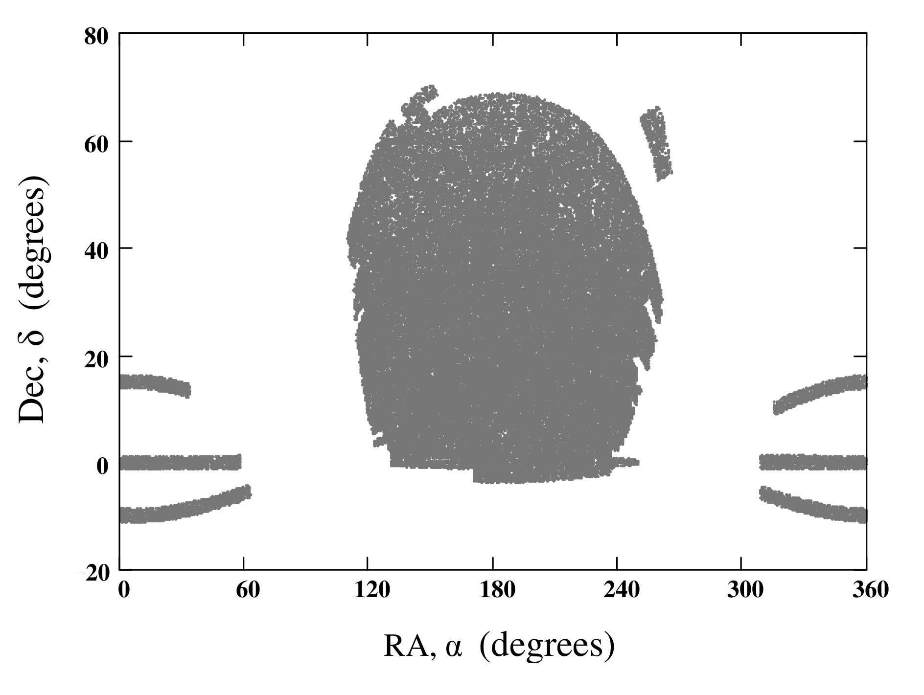
Fig. 1 : Angular distribution of LRGs from SDSS DR7 over the sky in the Equatorial coordinates; all grey coloured regions comprise DR7-Full sample of data (105 831 LRGs) represented in Table 1 by Kazin et al. (2010a); the data are available on the World Wide Web (see text).

The basic quantity of the present study is a radial distribution function N$({\eta})$ integrated over angles $\alpha$ (right ascension) and $\delta$ (declination), which is an analogue of the comoving number density $n(z)$ in the redshift space (e.g. Zehavi et al. 2005); $\eta(z)$ is a dimensionless line-of-site (radial) comoving distance between the observer and galaxies under study, N$(\eta)$d$\eta$ is a number of LRGs inside an interval d$\eta$.

The dimensionless radial comoving distances are calculated according to the equation (e.g. Harrison 1993, Kayser, Helbig & Schramm 1997, Hogg 1999):

$$\eta_{i}=\eta(z_{i})=\int_{0}^{z_{i}}{1\over\sqrt{\Omega_{\rm m}(1+z)^{3}+\Omega_{\rm\Lambda}}}\,\,{\rm d}z,$$ (1)

where $i$ is a numeration of all LRGs, $i=1,2,...,{\rm N}_{\rm tot}$, e.g., N${}_{\rm tot}=105831$ for the DR7-Full sample by Kazin et al. (2010a). Following Kazin et al. (2010a) we use the dimensionless density parameters $\Omega_{\rm m}=0.25$ and $\Omega_{\rm\Lambda}=1-\Omega_{\rm m}=0.75$. The corresponding line-of-sight comoving distances are  D${}_{{\rm c},i}=c\cdot\eta_{i}/H_{0}=2998\cdot\eta_{i}\cdot h^{-1}$ Mpc, where $H_{0}=100\leavevmode\nobreak\ h$ km s^-1 Mpc^-1 is the present Hubble constant, $c$ is the speed of light.

We focus our attention on the search of periodicities incorporated in the radial LRGs distribution in relation to the $\eta$-variable. We shall treat them as quasi-periodicities meaning limited intervals of line-of-sight distances under consideration, as well as variations of a peak positions and amplitudes for different samples of LRGs. In Section 2 we examine power spectra calculated for two samples of LRGs employing a point-like statistical approach: the full sample DR7-Full and a sample from the rectangle region described below. The point-like approach is usually used in order to avoid sensitivity of results to the procedure of a smoothed distribution function (trend) subtraction and to the related choice of an averaging bin. For comparison in Section 3 we discuss power spectra calculated in a binning approach for the DR7-Bright sample which is also represented in Table 1 by Kazin et al. (2010a). In Section 4 we use two mock galaxy LasDamas catalogues for more conservative estimations of significance levels of the power spectra, and outline shortly another (widely discussed) way to estimate the significance of the maximal peaks in the power spectra. Conclusions and discussions of the results are given in Section 5. Ambiguity effects of a trend elimination procedure on results of Fourier spectra analysis is shortly outlined in Appendix.

2 Quasi-periodicity of the $\eta$-distribution:
point-like approach

Fig. 2 demonstrates the radial distribution function N$(\eta)$ calculated for independent bins with a narrow width $\delta_{\eta}$ = 0.00033 or  $c\cdot\delta_{\eta}/H_{0}=1\leavevmode\nobreak\ h^{-1}$ Mpc at the scale of comoving distances. Narrow spike-like variations of N$(\eta)$ are noticeable on the background of the trend N${}_{\rm tr}(\eta)$ drawn by a thick solid line. The function N${}_{\rm tr}(\eta)$ can be treated as a smoothed function filtering out the largest scales (e.g. Zehavi et al. 2005, Kazin et al. 2010a). We assume that the trend can be determined by selection effects and/or large-scale fluctuations in the distribution of galaxies (e.g. Sylos Labini 2010). In Fig. 2 the function N${}_{\rm tr}(\eta)$ is calculated by the least-squares method using a set of parabolas as a regression function for N$(\eta)$.

Fig. 2 : Radial distribution function N$(\eta)$ of 105 831 LRGs belonging to the grey regions in Fig. 1 and a redshift interval $0.16\leq z\leq 0.47$ or dimensionless radial distances $0.16\leq\eta\leq 0.43$; N$(\eta)$ is calculated with using independent bins $\delta_{\eta}$ = 0.00033 or $c\cdot\delta_{\eta}/H_{0}=1\leavevmode\nobreak\ h^{-1}$ Mpc; thick solid line displays a trend N${}_{\rm tr}(\eta)$ determined as a set of parabolas (see text).

Our aim is to reveal weak but quite significant quasi-periodical components and separate them from the rest determinate part of the radial distribution (trend), as well as fluctuations. However, in the case of such a complex trend as displayed in Fig. 2 the procedure of the trend subtraction is ambiguous in principle and may bring to wide variations of peak positions and amplitudes in power spectra, as demonstrated in Appendix. So it is more safely in that case to employ an out-of-bin (point-like) statistical technique, which is not sensitive to the procedure of trend determination.

To verify the periodicity of the $\eta$-distribution we calculate a power spectrum for the sequence of LRG points $\eta_{i}\equiv\eta(z_{i})$ using the Rayleigh power: (e.g. Brazier 1994):

$${\rm P}({\rm m}) = {1\over{\rm N}_{\rm tot}}\left\{\left[\sum_{i=1}^{{\rm N}_{\rm tot}}\cos\left({2\pi{\rm m}\eta_{i}\over L_{\eta}}\right)\right]^{2}\right.$$ (2)

$$+ \left.\left[\sum_{i=1}^{{\rm N}_{\rm tot}}\sin\left({2\pi{\rm m}\eta_{i}\over L_{\eta}}\right)\right]^{2}\right\},$$

m is an integer harmonic number, L_η = $\eta_{max}-\eta_{min}$ is an interval under consideration. A periodicity yields a peak in the power spectrum ${\cal P}$=P(m), with the confidence probability or cumulative distribution function (e.g. Scargle 1982)

$$\beta=[1-\exp(-{\cal P})],$$ (3)

where $\beta$ is defined relative to the hypothesis of the Poisson distribution of $\eta_{i}$. This estimation is valid for a single independent peak at arbitrary m and yields the probability of pure noise generating a power P(m) less than given level ${\cal P}$.

Fig. 3 represents power-spectra P($k$) calculated with the use of Eq. (2) at $1\leq{\rm m}\leq 40$, where the wave number $k$ ($h$ Mpc^-1) substitutes for m according to an expression $k=2\pi{\rm m}/{\rm D}_{\rm c}^{\rm L}$, where ${\rm D}_{\rm c}^{\rm L}=c\cdot{\rm L}_{\eta}/H_{0}$ is the whole comoving interval. The upper and lower panels correspond to two overlapping samples of LRGs, both of them belong to the same interval $0.16\leq\eta\leq 0.43$ (L${}_{\eta}=0.27$,  D${}_{\rm c}^{\rm L}=809.4\leavevmode\nobreak\ h^{-1}$ Mpc). The upper panel is calculated for the whole region marked in Fig. 1 comprising the main sample of 105,831 LRGs, the lower one – for a rectangle region within the central oval-like domain restricted by the intervals of right ascension $140^{\circ}\leq\alpha\leq 230^{\circ}$ and declination $0\leq\delta\leq 60^{\circ}$. The region is chosen by analogy with Sylos Labini (2010) to minimize possible effects of the irregular edges of the central domain in Fig. 1. The latter sample contains 60,308 LRGs.

Fig. 3 : Power spectra P($k$) calculated in the point-like approach according to Eq. (2) for the redshift interval $0.16\leq z\leq 0.47$ ($0.16\leq\eta\leq 0.43$), $k$ is a wave number; the horizontal dash lines specify the significance levels 3$\sigma$, 4$\sigma$, and 5$\sigma$ estimated with the use of Eq. (3) at fixed levels of the confidence probability $\beta=0.998,\ 0.99994,\ 0.9999994$, respectively. Upper panel: P($k$) calculated for all LRGs from the grey regions in Fig. 1. Lower panel: P($k$) calculated for LRGs from a rectangle region inside the central oval-like domain in Fig. 1 restricted by intervals of right ascension, $140^{\circ}\leq\alpha\leq 230^{\circ}$, and declination, $0\leq\delta\leq 60^{\circ}$.

The most significant peaks of the spectra P($k$) are noticeable for two close periodicities at $k=0.047$ and $0.062\leavevmode\nobreak\ h$ Mpc^-1 or harmonic numbers m=6 and m=8. These values $k$ correspond to dimensionless radial comoving scales of $\eta$  $\Delta_{\eta}=0.045\pm 0.004$ and $0.034\pm 0.002$, or the comoving spatial scales $\Delta{\rm D}_{\rm c}=(135\pm 12)$ and $(101\pm 6)\leavevmode\nobreak\ h^{-1}$ Mpc, respectively. The latter peak (m=8) is dominant for both samples with amplitudes well exceeding the level 5$\sigma$ estimated with Eq. (3). While the first one (m=6) is somewhat less significant being lower than the level 5$\sigma$ for the rectangle region.

Fig. 4 demonstrates a reciprocal Fourier transform reconstructed for 5 harmonics from m=5 till m=9 and shown as a function of the comoving radial distance D_c. The appropriate direct Fourier transform including amplitudes and phases of harmonics is calculated for the sample of all LRGs from the grey regions in Fig. 1. One can see that the pair of close periodical components m=6 and m=8 yields a resultant quasi-periodical fluctuations of the radial distribution of LRGs. An averaged scale of the quasi-periodical fluctuations turns out to be $(100\pm 8)\leavevmode\nobreak\ h^{-1}$ Mpc, i.e. it is rather close to the main tone m=8.

Fig. 4 : Reciprocal Fourier transformation for five harmonic numbers $m$ (see Eq. (2)) from the interval $5\leq m\leq 9$ as a function of the comoving line-of-sight distance D_c. Vertical dash lines indicate positions of maxima of the reconstructed distribution. An averaged scale between neighbour dash lines is $(100\pm 8)\leavevmode\nobreak\ h^{-1}$ Mpc.

Less significant peaks are also visible in Fig. 3. A wide peak (significance 4$\sigma$) at $k=0.217\leavevmode\nobreak\ h$ Mpc^-1 (m=28), which is present in the both spectra, and a narrow peak at $k=0.124\leavevmode\nobreak\ h$ Mpc^-1 (m=16) appearing only in the lower panel. The first period corresponds to the spatial scale $\Delta{\rm D}_{\rm c}=$ $(29\,\,_{-2}^{+4})\leavevmode\nobreak\ h^{-1}$ Mpc. The second one, $(51\pm 2)\leavevmode\nobreak\ h^{-1}$ Mpc, turns out to be very close to the second harmonic of the main peak (m=8). Note a difference of the whole sets of spectral features for both samples under discussion.

Although the point-like approach avoids the procedure of a trend determination a steep rise of both the curves P($k$) at the lowest $k\;\raise 1.29167pt\hbox{$<$\kern-7.5pt\raise-4.73611pt\hbox{$\sim$}}\;0.05\leavevmode\nobreak\ h$ Mpc^-1 may be attributed to the effects of large-scale fluctuations incorporated in the smoothed $\eta$-dependence (see Fig. 2). On the other hand, the long-wave parts of the spectra are different for the two samples considered in Fig. 3. Such a difference appears, in particular, in relative decrease of the peak at $k=0.047\leavevmode\nobreak\ h$ Mpc^-1 and cancellation of spectral components within an interval of $0.03\;\raise 1.29167pt\hbox{$<$\kern-7.5pt\raise-4.73611pt\hbox{$\sim$}}\;k\;\raise 1.29167pt\hbox{$<$\kern-7.5pt\raise-4.73611pt\hbox{$\sim$}}\;0.04\leavevmode\nobreak\ h$ Mpc^-1 in the lower panel. The difference could be associated with effects of irregular edges of the oval-like region and a set of strips in Fig. 1 excluded in the rectangle region.

Our special simulations show that the point-like (out-of-bin) approach is more sensitive to the presence of periodicities in a distribution of points than the binning approach with relatively wide bins. The latter one needs an appropriate procedure of a trend subtraction. In the case of simple trends, e.g. close to linear or parabolic dependencies, amplitudes and positions of peaks in the power spectra calculated in the binning mode converge to the values found in the point-like approach at successive reducing of a bin width. This convergence can be demonstrated, e.g. for the narrow independent bins $\delta_{\eta}=0.00033$ used in Fig. 2. However, we found that in many cases both the convergent procedures yield overestimated significance of peaks in the power spectra. It suggests to re-estimate the significance levels of the spectral peaks in Fig. 3 in a more robust way than it can be produced with using Eq. (3). We realize this suggestion in Section 4.

3 Bright LRGs: binning approach

In the cases of quite simple trends (linear or parabolic functions) it is more relevant to use the binning approach and a proper procedure of a trend, N${}_{\rm tr}(\eta)$, subtraction. For instance, one can calculate so-called normalized radial distribution function:

$${\rm NN}(\eta)={{\rm N}(\eta)-{\rm N}_{\rm tr}(\eta)\over\sqrt{{\rm N}_{\rm tr}(\eta)}}.$$ (4)

Note that instead of the radial distribution function N$(\eta)$ one can use a comoving number density $n(\eta)={\rm N}(\eta)/({\rm d}{\rm V}/{\rm d}\eta)$, where ${\rm d}{\rm V}/{\rm d}\eta$ is a comoving differential volume, which is a simple variation of the more conventional value $n(z)$ (e.g., Zehavi et al. 2005, Kazin et al. 2010a). This replacement does not change Eq. (4) and results of following calculations because in that case one should divide into the comoving volume both numerator and denominator (remind that $\sigma(n)=\sigma(N)/{\rm V}$, where $\sigma$ is the mean squared deviation).

An example of quite simple trend is demonstrated in the upper panel of Fig. 5. We explore the DR7-Bright sample indicated in Table 1 by Kazin et al. (2010a), which contains 33,356 SDSS “Bright” LRGs ($-23.2<M\leq-21.8$,  $M$ is the absolute magnitude) within a redshift interval $0.16\leq z\leq 0.44$ ($0.155\leq\eta\leq 0.40$). The upper panel in Fig. 5 displays the function N$(\eta)$ calculated for the same independent bins ($\delta_{\eta}=0.00033$) as in Fig. 2. The trend N${}_{\rm tr}(\eta)$ is calculated as a parabolic function by the least-squares method and drawn by a thick solid line.

The middle panel in Fig. 5 represents the power spectrum obtained for NN$(\eta)$ according to the equation:

$${\rm P}_{\rm b}(k) = {1\over{\cal N}_{\rm b}}\left\{\left[\sum_{j=1}^{{\cal N}_{\rm b}}{\rm NN}_{j}\cos\left({2\pi{\rm m}\eta_{j}\over L_{\eta}}\right)\right]^{2}\right.$$ (5)

$$+ \left.\left[\sum_{j=1}^{{\cal N}_{\rm b}}{\rm NN}_{j}\sin\left({2\pi{\rm m}\eta_{j}\over L_{\eta}}\right)\right]^{2}\right\},$$

where ${\cal N}_{\rm b}$ is a number of bins along $\eta$-axis, $\eta_{j}$ is a location of bin centers, $\eta_{j}\pm\delta_{\eta}/2$;   $j=1,2,...,{\cal N}_{\rm b}$ numerates bins, in the case of the middle panel ${\cal N}_{\rm b}=736$,  L_η = $\eta_{max}-\eta_{min}=0.245$ (or ${\rm D}_{\rm c}^{\rm L}=735\leavevmode\nobreak\ h^{-1}$ Mpc) is the whole interval.

Fig. 5 : Upper panel: Radial distribution function N$(\eta)$ calculated for a sample of SDSS “Bright” LRGs ($-23.2<M\leq-21.8$) within a redshift interval $0.16\leq z\leq 0.44$ ($0.155\leq\eta\leq 0.4$) indicated as DR7-Bright in Table 1 by Kazin et al. (2010a). N$(\eta)$ is calculated with using the same independent bins ($\delta_{\eta}$ = 0.00033) as in Fig. 2; solid thick line displays a smoothed function (trend) N${}_{\rm tr}(\eta)$ drawn as 2^d-degree polynomial. The whole sample contains 33,356 LRGs. The vertical dash line shows a shifted low boundary $\eta$ for a reduced sample of the “Bright” LRGs. Middle panel: Power spectrum P${}_{\rm b}(k)$ of the function NN$(\eta)$ calculated according to Eq. (5) for the whole sample. Lower panel: Similar power spectrum P${}_{\rm b}(k)$ but calculated for the reduced sample of 32,395 LRGs with shifted low boundary: $0.172\leq\eta\leq 0.4$. The horizontal dash lines indicate the same significance levels as in Fig. (3)

The power spectrum contains two significant peaks exceeding the level $3\sigma$ at $k=$ 0.017 and 0.120 $h$ Mpc^-1. The first peak (m=2) corresponds to a half of the whole interval and may be interpreted as a residual large-scale fluctuation which could be incorporated into the trend N${}_{\rm tr}(\eta)$ but it is missed out by the parabolic approximation. The second peak corresponds to a period of $\Delta{\rm D}_{\rm c}=(52.5\pm 2)\leavevmode\nobreak\ h^{-1}$ Mpc, and may be compared with the peak $k=0.124\leavevmode\nobreak\ h$ Mpc^-1 in the lower panel of Fig. 3.

The lower panel in Fig. 5 shows a complementary power spectrum calculated in the same way but for a somewhat diminished sample of 32,395 “Bright” LRGs within a reduced redshift interval $0.18\leq z\leq 0.44$ ($0.172\leq\eta\leq 0.40$), i.e. lower edge is shifted. Thus in calculations with Eq. (5) we use the values ${\cal N}_{\rm b}=685$,  L_η = $\eta_{max}-\eta_{min}=0.228$. Similar to the middle panel the power spectrum contains two significant peaks at $k=$ 0.018 and 0.120 $h$ Mpc^-1. The first peak, slightly shifted in respect of the peak in the middle panel, implies the same interpretation. The second one displays the same period as the full sample of “Bright” LRGs but with higher amplitude ($\;\raise 1.29167pt\hbox{$>$\kern-7.5pt\raise-4.73611pt\hbox{$\sim$}}\;4\sigma$). The difference between two spectra may be treated as an edge effect which provides better tuning of the Fourier component at $k=0.12\leavevmode\nobreak\ h$ Mpc^-1 in the case of reduced sample.

Comparing Figs. 5 and  3 one can notice that the power spectra are strongly dependent on a sample of objects under investigation. In particular, the radial distribution of the bright LRGs displays the peak structure of the power spectrum which differs from that obtained for the whole sample.

4 Significance estimations: LasDamas catalogues

In this Section we employ two mock galaxy LasDamas (LD) catalogs “lrgFull-real” and “lrg21p8-real” (the latter simulates SDSS sample of bright LRGs with $M\leq-21.8$) for complementary estimations of the significance of spectral peaks appearing in Figs. 3 and 5. In both cases we use the data of 80 “ns” (North-South) realizations. Our aim is to take into account possible clustering of the galaxy distribution incorporated in the mock LD catalogs (e.g. Berlind & Weinberg 2002, see also Manera et al. 2012) in contrast to the hypothesis of Gaussian fluctuations used in Sections 2 and 3. We calculate power spectra for all realizations of both LD catalogs and approximate the whole array of spectra by the unified $\chi^{2}$-distribution applied to spectral amplitudes at each harmonic number m (wave number $k$) under investigation. Quality of the a approximation for each m or $k$ is controlled by the Kolmogorov criteria with a tabulated value $\lambda_{1-p}$ at fixed significance level $p=0.2$ ($\lambda_{0.8}=1.07$).

Fig. 6 : Power spectra for two samples of LRGs discussed in Sections 2 and 3 in comparison with appropriate significance levels (dash lines) and mean power spectra (thin solid lines) calculated on the basis of LasDamas mock catalogs (see text for details). Upper panel: same power spectrum P$(k)$ as in the upper panel of Fig. 3; significance levels of $2\sigma$, $3\sigma$ and $4\sigma$, as well as the mean spectral line, are calculated with the use of 80 realizations of LasDamas “lrgFull-real” catalog. Lower panel: same power spectrum P${}_{\rm b}(k)$ as in the middle panel of Fig. 5; significance levels of $2\sigma$ and $3\sigma$, as well as the mean spectral line, are calculated with the use of 80 realizations of LasDamas “lrg21p8-real” catalog.

To obtain two sets of the power spectra we perform calculations of the radial distributions of the LD galaxies with using of the binning approach. We employ the same bin $\delta_{\eta}$ = 0.00033 as in Section 3. As it was discussed in Section 2 the power spectra calculated with such a small bin in the case of a simple trend display insignificant difference with the power spectra obtained in the point-like approach. This allows one to apply significance levels estimated on the base of LD data to the point-like statistics used in Section 2.

To make statistical properties of the mock samples of the “lrgFull-real” catalog more comparable with the main sample of LRGs used in Section 2 we implement a reduction of the data, which reconciles simple radial selection functions (trends) N${}_{\rm tr}^{\rm LD}(\eta)$ of the LD data with the complex trend of the LRG sample. The procedure of the reduction is performed for all realizations of the LD catalog within the interval $0.16\leq\eta\leq 0.40$ according to the formula:

$$N_{fin}(\eta_{j})=N_{in}(\eta_{j})\times{\rm N}_{\rm tr}^{\rm SDSS}(\eta_{j})/{\rm N}_{\rm tr}^{\rm LD}(\eta_{j});$$ (6)

where $\eta_{j}$ is a centre of j-th independent bin, N${}_{in}(\eta_{j})$ and N${}_{fin}(\eta_{j})$ are initial and final radial distributions of mock galaxies over all independent bins, N${}_{\rm tr}^{\rm SDSS}(\eta_{j})$ is a trend of the radial distribution calculated for the main SDSS sample, N${}_{\rm tr}^{\rm LD}(\eta_{j})$ is a linear trend calculated for each mock realization. For the whole sample of 105,831 LRGs we calculate a trend N${}_{\rm tr}^{\rm SDSS}(\eta_{j})$ as a reciprocal Fourier transformation of the first five harmonics (m=1, …, 5) with their amplitudes and phases obtained in the direct Fourier transform. This trend is shown in Fig. 8 of Appendix.

Then the normalized radial distributions NN_j can be determined by Eq. (4), where N${}_{fin}(\eta_{j})$ and a mean value $\overline{\rm N}_{fin}$ stand for N$(\eta)$ and N${}_{\rm tr}(\eta)$, respectively. The mean $\overline{\rm N}_{fin}$ over the interval $0.16\leq\eta\leq 0.40$ is used as the simplest trend to bring the binning approach of Eq. (5 ) closer to the point-like approach of Eq. (2). It allows us to compare statistically a resultant sample of the mock power spectra obtained for all realizations of the “lrgFull-real” catalog with the spectrum in the upper panel of Fig. 3.

For the samples of the “lrg21p8-real” mock catalog we also employ the procedure described in Section 3 with the use of N${}_{in}(\eta_{j})$ and the parabolic trend N${}_{\rm tr}(\eta_{j})$ for calculations of the values NN_j. Following Eq. (5) we obtain a set of power spectra and compare the distributions of their amplitudes with the power spectrum in the middle panel of Fig. 5.

It was found with the use of the Kolmogorov criterion that the $\chi^{2}$-distribution of peak amplitudes P($k$) is valid for a majority (but not all) of $k$ in the power spectra obtained for “lrgFull-real” and “lrg21p8-real” realizations. Specifying the confidence probability $\beta$ we calculate the significance levels of P($k$) at each $k=2\pi m/{\rm D}_{\rm c}^{\rm L}$, determined by all integer ${\rm m}_{min}\leq{\rm m}\leq 40$; it is performed within the interval $0.04\leq k\leq 0.25\leavevmode\nobreak\ h$ Mpc^-1 (m${}_{min}=5$) for the whole SDSS LRG sample and at $0.017\leq k\leq 0.25\leavevmode\nobreak\ h$ Mpc^-1 (m${}_{min}=2$) for the “Bright” LRGs.

Results of the statistical estimations of the peaks significance for both SDSS LRG samples are represented in Fig. 6. The upper panel displays the same power spectrum as in the upper panel of Fig. 3 and the lower panel corresponds to the middle panel of Fig. 5. Thin solid lines in both panels are drawn through arithmetical means of peak amplitudes calculated for each m (${\rm m}_{min}\leq{\rm m}\leq 40$) or respective $k$ for the appropriate sets of power spectra. Dashed lines in both panels are drawn through significance levels $2\sigma$, $3\sigma$, and $4\sigma$ (upper panel) calculated as the amplitudes P$(k)$ at all respective $k$ matching with the confidence probabilities of the $\chi^{2}$-distributions: $\beta=0.95$, $\beta=0.998$, and $\beta=0.99994$, respectively. Let us note that our model estimations are quite approximate due to lack of statistics of the mock catalogs and may underestimate real significance of the peaks.

In the upper panel of Fig. 6 one can see only two peaks $k=0.047$ and 0.062 $h$ Mpc^-1 exceeding the significance level $3\sigma$, the latter one is higher than $4\sigma$. The significance of the third peak $k=0.217\leavevmode\nobreak\ h$ Mpc^-1 hardly approaches to the level $3\sigma$ in contrast with its level ($4\sigma$) in Fig. 3. Three noticeable peaks in the lower panel of Fig. 6 turn out to be less significant ($\;\raise 1.29167pt\hbox{$>$\kern-7.5pt\raise-4.73611pt\hbox{$\sim$}}\;2\sigma$). However, the growth of the peak at $k=0.12\leavevmode\nobreak\ h$ Mpc^-1 in the lower panel of Fig. 5 as well as an appearance of the peak at $k\approx 0.12\leavevmode\nobreak\ h$ Mpc^-1 in the lower panel of Fig. 3 give an evidence in favour of possible presence of the additional comoving scale $\Delta{\rm D}_{\rm c}=(52.5\pm 4)\leavevmode\nobreak\ h^{-1}$ Mpc in the radial distribution of LRGs. This peak should be confirmed or rejected by further investigations with extended statistics.

It was marked in Section 2 that the estimations of the confidence probability according to Eq. (3) imply appearance of a single peak at some wave number $k$ in a power spectrum with an amplitude ${\cal P}$. Following Scargle (1982) (see also Frescura, Engelbrecht, Frank 2008 and references therein) one can consider a set of many independent wave numbers $k_{m}$; m$=1,...,N_{k}$, where $N_{k}$ may be $\gg 40$ used in Fig. 3, and treat any of power peaks P(m) as a result of Gaussian noise. Then one can estimate so called false alarm probability, $F={\rm Pr}({\rm P}_{max}\geq{\cal P})=1-\beta^{N_{k}}$, where $\beta$ is defined in Eq. (3), i.e. probability of at least one of peaks P_max being equal to (or above) a maximal level ${\cal P}$.

Considering a set of natural wave numbers $k\propto$m for the whole sample of LRGs in Figs. 3 and 6 we regard that $N_{k}$ is close to the theoretical value ${\cal N}_{\rm b}/2$ (Frescura, Engelbrecht, Frank 2008) and exploit also the proximity of the point-like and binning approaches at the same $\delta_{\eta}$ = 0.00033. One can deal with the normalized power amplitude P${}_{max}={\cal P}=26.4$ at k$=0.062$ and use the formula ${\cal P}_{0}=-ln[1-(1-p_{0})^{1/N_{k}}]$ (Scargle 1982, Frescura, Engelbrecht, Frank 2008) ) to match a given level of the false alarm probability $p_{0}$ with an amplitude ${\cal P}_{0}$. In our case ${\cal N}_{\rm b}=818$, $N_{k}=409$  and we obtain that the confidence level $(1-p_{0})=0.9999994$ (significance $5\sigma$) corresponds to ${\cal P}_{0}=20.3$. Thus the obtained value lies between the $5\sigma$-level in Fig. 3 ($\;\raise 1.29167pt\hbox{$<$\kern-7.5pt\raise-4.73611pt\hbox{$\sim$}}\;15$) and the amplitude 26.4 mentioned above. The estimation makes the significance of the main peak lower but not so much lower as the $4\sigma$-level in Fig. 6.

Analogous estimations can be carried out with the power peak at $k=0.12$ in the middle panel of Fig. 5. The confidence probability of the peak $1-p_{0}=0.986$ also becomes lower (significance $<3\sigma$). In general, the estimations employing the false alarm probability yield systematically lower confidence levels of the maximal power peaks, but these levels are higher than the estimations on the base of LD mock catalogs discussed above. Therefore we treat the single-peak estimations with using Eq. (3) and the LD-estimations as maximal and minimal boundaries of possible confidence levels.

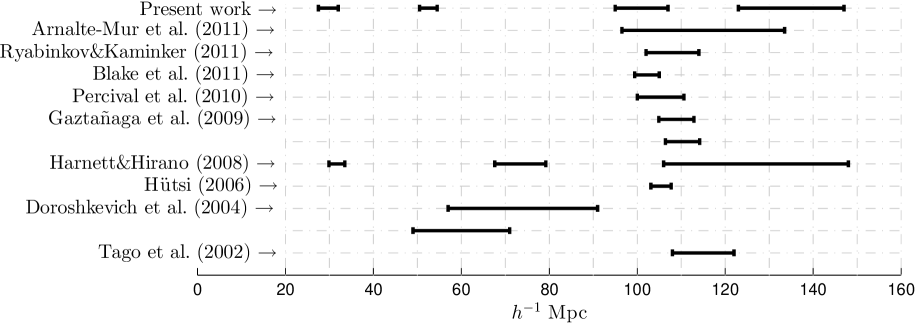
Fig. 7 : Cosmological characteristic scales obtained in the last decade by a few groups of authors, the references are indicated in the left column. Horizontal segments depict uncertainties indicated by the authors except the error bar attributed to the results of Percival et al. (2010) (at $\Omega_{\rm m}=0.28$,  $z=0.2$), which we estimated on the basis of data given in the cited paper. The error bar related to the results of Arnalte-Mur et al. (2011) is also introduced rather arbitrary on basis of their Figure 2.

5 Conclusions and discussion

The main conclusions of the statistical analysis of radial (line-of-sight) distributions of the LRGs within the redshift interval $0.16\leq z\leq 0.47$ or the interval of dimensionless line-of-sight comoving distance $0.16\leq\eta\leq 0.43$ can be summarized as follows:

(1) The radial distribution of $\sim$ 106,000 LRGs incorporates a few ($\leq 4$) significant quasi-periodical components in relation to the smoothed function (trend). The most significant peaks of the power spectra are displayed for two close periodicities corresponding to the spatial characteristic scales $(135\pm 12)$ and $(101\pm 6)\leavevmode\nobreak\ h^{-1}$ Mpc. The latter scale is a dominant with significance $\;\raise 1.29167pt\hbox{$>$\kern-7.5pt\raise-4.73611pt\hbox{$\sim$}}\;4\sigma$. This pair of close periodical components may be treated as an integrated quasi-periodical scale ($100\pm 8)\leavevmode\nobreak\ h^{-1}$ Mpc.

(2) Once more appreciable quasi-periodical scale, $(29\,\,_{-2}^{+4})\leavevmode\nobreak\ h^{-1}$ Mpc, arises in the power spectra as a wide peak at a level $\;\raise 1.29167pt\hbox{$>$\kern-7.5pt\raise-4.73611pt\hbox{$\sim$}}\;3\sigma$. The peak displays similar amplitudes for two overlapping samples: the main sample of 105,831 LRGs and a sample of 60,308 LRGs from the rectangle region (see Sect. 2). Still less reliable scale $(52.5\pm 4.0)\leavevmode\nobreak\ h^{-1}$ Mpc appears for the sample of LRGs from the rectangle-region and for the sample of “Bright” LRGs. These periodicities must be verified by further examinations.

(3) The main quasi-periodical scale found in this work ($(101\pm 6)\leavevmode\nobreak\ h^{-1}$ Mpc) is consistent with the scale $(102.2\pm 2.8)\leavevmode\nobreak\ h^{-1}$ Mpc of the baryon acoustic peak in the two-point (monopole) correlation function of the LRG distribution (Blake et al. 2011). These scales are in agreement also with a period of $(108\pm 6)\leavevmode\nobreak\ h^{-1}$ Mpc revealed by Ryabinkov & Kaminker (2011) in the radial distribution of QSO ALSs for a wider redshift interval $0.0\leq z\leq 4.3$. Note that the nearness of the periods $\sim 100h^{-1}$ Mpc revealed at redshifts $z\;\raise 1.29167pt\hbox{$<$\kern-7.5pt\raise-4.73611pt\hbox{$\sim$}}\;0.5$ for LRGs and at $z\leq 4.3$ for QSO ALSs argues for spreading of the same large-scale periodicity over long interval of the cosmological evolution (see also Demiański et al. 2011).

(4) A set of peaks in the power spectra of Figs. 3, 5 and their variations from sample to sample probably evidence in favour of rather spatial than temporal nature of the quasi-periodicities discussed here. Our model simulations performed for partly ordered structures of points (e.g., Ryabinkov & Kaminker 2011) show that it is possible to get a point-like power spectra similar to those represented in Figs. 3 and 5 performing simulations of a cloud-like 3D-distribution of points around vertices, e.g. of a face-centered cubic.

(5) On the other hand, we can not eliminate also an alternative interpretation which may be conventionally denominated as the temporal one, i.e. generation of some temporal wave processes in the course of the cosmological evolution (e.g. Morikawa 1991; Aref’eva & Koshelev 2008; Hirano & Komiya 2010). Although, it seems to be more difficult to explain a temporal structure formed by more-than-one periodical processes. Note, however, that one temporal interval $\Delta{\rm T}_{\rm c}=\Delta{\rm D}_{c}/c=$ $(330\pm 30)\leavevmode\nobreak\ h^{-1}$ Myr corresponding to the main quasi-periodicity indicated above could be consistent with the results of Aref’eva & Koshelev (2008).

Let us note that results of our analysis could be quite sensitive to possible radial incompleteness of the DR7-Full sample. It is likely that some fainter LRGs at larger redshifts were missed by the survey. To minimize such a selection Kazin et al. (2010a) restricted their analysis by redshifts $z\sim 0.36$ corresponding to the quasi-volume-limited sample. They performed additionally some angular and radial weighting procedures and showed that their results did not variate essentially. Using the same catalog Blake et al. (2011) extended similar analysis to higher redshifts $z=0.44$ and obtained the close peak position in the correlation function. Here we analyse the whole DR7-Full sample of LRGs up to $z_{max}=0.47$. However, as it seen in Fig. 2 the distribution function N$(\eta)$ is still quite representative at the edge of highest $\eta$. All that may evidence in favour of an assumption that at least the scales $\sim 100\leavevmode\nobreak\ h^{-1}$ Mpc are not distorted strongly by the radial-selection effects.

Fig. 7 gives examples of characteristic scales which have been obtained in the last decade by a few groups of authors as a result of analysis of large-scale distributions of galaxies and galaxy clusters. A part of data displayed in Fig. 7 is taken from Table 1 of Ryabinkov & Kaminker (2011). Additional segments of scales are introduced with using results of Hütsi (2006) on the BAO incorporated in the power spectrum of the SDSS DR4 LRG sample, and Percival et al. (2010) on the disclosure of the BAO in the power spectra of both SDSS DR7 samples: LRGs and MGS, with inclusion of 2dF Galaxy Redshift Survey data. We add also the recent results by Arnalte-Mur et al. (2011) on the wavelet analysis of acoustic wave features in the spatial galaxy distribution.

Fig. 7 should be considered only as an illustration and it includes rather nonuniform results. For instance, Tago et al. (2002) yielded a characteristic period, $(115\pm 7)\leavevmode\nobreak\ h^{-1}$ Mpc, of regular spatial oscillations of the two-point correlation function calculated for galaxy superclusters (see also Einasto et al. 1997a, b). Two scale intervals chosen from Table 1 of Doroshkevich et al. (2004) correspond to the mean separations between walls – the largest elements of the Large Scale Structure (LSS) in the galaxy distribution. The scale $(74\pm 17)\leavevmode\nobreak\ h^{-1}$ Mpc was obtained on the basis of radial (line-of-sight) measurements with using data of SDSS DR1 catalog (at $z\leq 0.14$), while the scale $(60\pm 10)\leavevmode\nobreak\ h^{-1}$ Mpc corresponds to the Las Campanas Redshift Survey data (at $z\leq 0.11$). Three significant periods, $(127\pm 21)\leavevmode\nobreak\ h^{-1}$ Mpc, $(73.4\pm 5.8)\leavevmode\nobreak\ h^{-1}$ Mpc, and $(31.7\pm 1.8)\leavevmode\nobreak\ h^{-1}$ Mpc, were revealed by Hartnett & Hirano (2008) in their Fourier analysis of radial galaxy distribution on the basis of SDSS DR5 and 2dF GRS data. The periodicity found by Ryabinkov & Kaminker (2011) in the radial distribution of QSO ALSs is also included.

In spite of heterogeneity of the results, the scales in Fig. 7 may be formally subdivided into three groups: two scales belong to the interval $(30\pm 3)\leavevmode\nobreak\ h^{-1}$ Mpc, four scales belong to the wider interval $(70\pm 21)\leavevmode\nobreak\ h^{-1}$ Mpc, and the most representative interval is $(121\pm 26)\leavevmode\nobreak\ h^{-1}$ Mpc. Four periodical components discussed in the present paper get into these intervals; two most significant periods of our analysis belong to the third group. Especially good agreement of the main scale , $(101\pm 6)\leavevmode\nobreak\ h^{-1}$ Mpc, occurs with results obtained by Blake et al. (2011), Kazin et al. (2010a), Percival et al. (2010), and Hütsi (2006) for the BAO scale.

Actually, BAOs are discussed in literature as a scale of the sound horizon at the recombination epoch (e.g. Blake & Glazebrook 2003; Percival et al. 2007b) displaying itself as a single feature in the spatial correlation function (e.g. Eisenstein et al. 2005; Kazin et al. 2010a; Blake et al. 2011). This feature appears also as a series of regular variations (oscillations) imprinted in the power spectrum calculated for the spatial 3D-distribution of galaxies (e.g. Eisenstein & Hu 1998; Eisenstein, Hu & Tegmark 1998; Hütsi 2006; Percival et al. 2010; Ross et al. 2012). They principally differ from the quasi-regular variations of the radial (1D) distributions in real space discussed by Ryabinkov & Kaminker (2011) and the present paper. However, it is not unlikely that both types of variations could be reconciled.

The radial distribution variations probably bring out some spatial partly-ordered structure of matter in the early Universe (e.g. Einasto et al. 1997b; Einasto et al. 2011) characterized by a long-range (or intermediate-range) order. In particular, one can admit the possibility that primordial acoustic perturbations, responsible for the BAO, could carry traces of a partly ordering formed at some early epochs (e.g. radiation-matter equipartition or recombination). In that case the radial (1D) distributions, as well as the two-point 3D-space correlation function, would display a set of quasi-periodic features, which might reveal itself into a complex set of features (e.g. peaks) in appropriate power spectra. Note that possible presence of the second feature in the two-point correlation function at a scale approximately double to the BAO scale $\sim 200\leavevmode\nobreak\ h^{-1}$ Mpc has been revealed recently by Ross et al. (2012); see also Martínez et al. (2009).

In any case, the existence of the large-scale periodicities, as well as the space-ordering hypothesis, needs further verifications based on statistical properties of different cosmological objects over wider redshift regions.

Acknowledgments The work has been supported partly by the RFBR (grant No.  11-02-01018-a), by the State Program “Leading Scientific Schools of Russian Federation” (grant NSh 4035.2012.2), as well as by Ministry of Education and Science of Russian Federation (contract No. 11.G34.31.0001 and agreement No. 8409).

Appendix A Effects of trend uncertainties

Fig. 8 demonstrates variations of the power spectra obtained with using different procedures of the radial smoothed function (trend) subtraction (see Sect. 3). We examine 105 831 LRGs from DR7-Full sample represented in Table 1 by Kazin et al. (2010a). The upper panel in Fig. 8 is designed similar to Fig. 2 but with using three different ways of the trend determination. In all cases the radial (line-of-sight) distribution function N$(\eta)$ is calculated for independent bins $\delta_{\eta}$ = 0.00033 or  $c\cdot\delta_{\eta}/H_{0}=1\leavevmode\nobreak\ h^{-1}$ Mpc providing narrow spike-like variations of N$(\eta)$. The first trend function N${}_{\rm tr}(\eta)$ is calculated by the least-squares method with using a set of parabolas (thick solid line) as a regression function for N$(\eta)$. The second one is calculated as a sum of the first five reciprocal Fourier harmonics, m=1, …, 5 (thick dashed line), with full filtration of all the rest harmonics $6\leq{\rm m}\leq 40$. The third trend is calculated with using the radial selection function $n(z)$ by Kazin et al. (2010a) presented on the World Wide Web (see Sect. 1). We rescale $n(z)$ into N${}_{\rm tr}(\eta)$ and applicate a spline interpolation for additional smoothing of the trend function (dotted line). Let us emphasize that $\chi^{2}$-criterion does not admit to prefer one of three trends although the results of power spectrum calculations for each of them are qualitatively different.

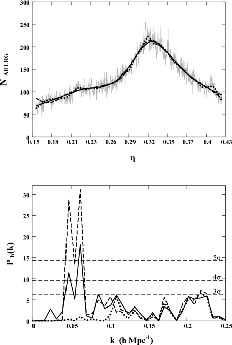
Fig. 8 : Effects of a procedure of smoothed function (trend) determination on appropriate power spectra calculated in the binning approach. Upper panel: same radial distribution function N$(\eta)$ as in Fig. 2 but with three different trends: solid line – set of parabolas (same as N${}_{\rm tr}(\eta)$ in Fig. 2), dashes – reciprocal Fourier transform employing first five harmonics, dots – radial selection function obtained from a comoving number density $n(z)$ of Kazin et al. (2010a) with carrying out a spline interpolation. Lower panel: three power spectra calculated with using Eqs. 4,  5 and the trends displayed in the upper panel by the respective type of lines.

The lower panel displays the respective power spectra calculated with Eqs. (4) and (5) and depicted by the same type of lines. One can see how the two most significant peaks at $k=0.062\leavevmode\nobreak\ h$ Mpc^-1 (m=8) and $k=0.047\leavevmode\nobreak\ h$ Mpc^-1 (m=6) strongly depend on a trend obtained in one of the ways indicated above: the features may variate from strong double peak (dashed line) up to its cancellation (dotted line). Whereas for $k\;\raise 1.29167pt\hbox{$>$\kern-7.5pt\raise-4.73611pt\hbox{$\sim$}}\;0.1$, i.e. for shorter waves, the effects of different trends are less essential. One can notice that in the upper panel the spline interpolation of the trend (dots) displays long-wave oscillations and thus compensates the corresponding Fourier harmonics. To some degree such a compensation may occur for different trends subject to their sufficient complexity. The oscillations inherent in trends can have also as physical as nonphysical origin and in their turn need special statistical considerations.

The indicated uncertainties make the binning approach, including a procedure of the trend subtraction, quite ambiguous at least in the cases of complex trends. Therefore, one needs a verification by a few statistical tests additional to the binning approach discussed in Sect. 3, including the point-like treatment, to make more robust conclusions concerning reality of quasi-periodicities in the distribution of matter.

References

- Abazajian et al. (2009) Abazajian K. N. et al., 2009, Astrophys. J. Suppl. Ser., 182, 543
- Aref’eva & Koshelev (2008) Aref’eva I. Ya., Koshelev A. S., 2008, JHEP, 9, 68 (arXiv:0804.3570)
- Arnalte-Mur et al. (2011) Arnalte-Mur P., Labatie A., Clerc N., Martínez V. J., Starck J-L., Lachièze-Rey M., Saar E., Paredes S. 2011, preprint (arXiv:1101.1911)
- Berlind & Weinberg (2002) Berlind A. A., Weinberg D. H., 2002, Astrophys. J., 575, 587
- Blake & Glazebrook (2003) Blake C., Glazebrook K., 2003, Astrophys. J., 594, 665
- Blake et al. (2011) Blake C. et al., 2011, Mon. Not. R. Astron. Soc., 418, 1707
- Brazier (1994) Brazier K. T. S., 1994, Mon. Not. R. Astron. Soc., 268, 709
- Cabré & Gaztañaga (2009) Cabré A., Gaztañaga E., 2009, Mon. Not. R. Astron. Soc., 393, 1183
- Demiański et al. (2011) Demiański M., Doroshkevich A., Pilipenko S., Gottlöber S., 2011, Mon. Not. R. Astron. Soc., 414, 1813
- Doroshkevich et al. (2004) Doroshkevich A. G., Tucker D. L., Allam S., Way M. J., 2004, Astron. Astrophys., 418, 7
- Einasto et al. (1997a) Einasto J. et al., 1997a, Mon. Not. R. Astron. Soc., 289, 801
- Einasto et al. (1997b) Einasto J., Einasto M., Frisch P., Gottlöber S., Müller V., Saar V., Starobinsky A. A., Tucker D., 1997b, Mon. Not. R. Astron. Soc., 289, 813
- Einasto et al. (2011) Einasto J. et al., 2011, Astron. Astrophys., 531, 75, preprint (arXiv:1012.3550)
- Eisenstein & Hu (1998) Eisenstein D. J., Hu W., 1998, Astrophys. J., 496, 605
- Eisenstein, Hu & Tegmark (1998) Eisenstein D. J., Hu W., Tegmark M., 1998, Astrophys. J. Lett., 504, L57
- Eisenstein et al. (2001) Eisenstein D. J. et al., 2001, Astron. J., 122, 2267
- Eisenstein et al. (2005) Eisenstein D. J. et al., 2005, Astrophys. J., 633, 560
- Frescura, Engelbrecht, Frank (2008) Frescura F. A. M., Engelbrecht C. A., Frank B. S., 2008, Mon. Not. R. Astron. Soc., 388, 1693
- Gaztañaga, Cabré & Hui (2009) Gaztañaga E., Cabré A., Hui L., 2009, Mon. Not. R. Astron. Soc., 399, 1663
- Harrison (1993) Harrison E., 1993, Astrophys. J., 403, 28
- Hartnett & Hirano (2008) Hartnett J. G., Hirano K., 2008, Astrophys. Space Sci., 318, 13
- Hirano & Komiya (2010) Hirano K., Komiya Z., 2010, Phys. Rev. D, 82, 103513
- Hogg (1999) Hogg D.W., 1999, preprint (astro-ph/9905116)
- Hütsi (2006) Hütsi G., 2006, Astron. Astrophys., 449, 891
- Kazin et al. (2010a) Kazin E. A. et al., 2010a, Astrophys. J., 710, 1444, preprint (arXiv:0908.2598)
- Kazin et al. (2010b) Kazin E. A., Blanton M. R., Scoccimarro R., McBride C. K., Berlind A. A., 2010b, Astrophys. J., 719, 1032, preprint (arXiv:1004.2244)
- Kayser, Helbig & Schramm (1997) Kayser R., Helbig P., Schramm T., 1997, Astron. Astrophys., 318, 680
- Manera et al. (2012) Manera M. et al., 2012, preprint (arXiv:1203.6609)
- Martínez et al. (2009) Martínez V. J., Arnalte-Mur P., Saar E., De la Cruz P., Pons-Bordería M. J., Paredes S., Fernández-Soto A., Tempel E., 2009, Astrophys. J. Lett., 696, L93
- Morikawa (1991) Morikawa M., 1991, Astrophys. J., 369, 20
- Percival et al. (2007a) Percival W. J., Cole S., Eisenstein D. J., Nichol R. C., Peacock J. A., Pope A.C., Szalay A. S., 2007a, Mon. Not. R. Astron. Soc., 381, 1053
- Percival et al. (2007b) Percival W. J. et al., 2007b, Astrophys. J., 657, 51
- Percival et al. (2010) Percival W. J. et al., 2010, Mon. Not. R. Astron. Soc., 401, 2148
- Ross et al. (2012) Ross A. J. et al., 2012, Mon. Not. R. Astron. Soc., 424, 564
- Ryabinkov & Kaminker (2011) Ryabinkov A. I., Kaminker A. D., 2011, Astrophys. Space Sci., 331, 79
- Sánchez et al. (2009) Sánchez A.G. Crocce M., Cabré A., Baugh C.M., Gaztañaga E., 2009, Mon. Not. R. Astron. Soc., 400, 1643
- Scargle (1982) Scargle J. D., 1982, Astrophys. J., 263, 835
- Sylos Labini et al. (2009a) Sylos Labini F., Vasilyev N.L., Baryshev Y.V., López-Corredoira M., 2009a, Astron. Astrophys., 505, 981
- Sylos Labini, Vasilyev & Baryshev (2009b) Sylos Labini F., Vasilyev N.L., Baryshev Y.V., 2009b, Astron. Astrophys., 496, 7
- Sylos Labini (2010) Sylos Labini F., 2010, preprint (arXiv:1011.4855)
- Tago et al. (2002) Tago E., Saar E., Einasto J., Einasto M., Müller V., Andernach H., 2002, Astron. J., 123, 37
- York et al. (2000) York D. G. et al., 2000, Astron. J., 120, 1579
- Zehavi et al. (2005) Zehavi I. et al., 2005, Astrophys. J., 621, 22