Effects of community structure on epidemic spread in an adaptive network

Abstract

When an epidemic spreads in a population, individuals may adaptively change the structure of their social contact network to reduce risk of infection. Here we study the spread of an epidemic on an adaptive network with community structure. We model the effect of two communities with different average degrees. The disease model is susceptible-infected-susceptible (SIS), and adaptation is rewiring of links between susceptibles and infectives. The bifurcation structure is obtained, and a mean field model is developed that accurately predicts the steady state behavior of the system. We show that an epidemic can alter the community structure.

I Introduction

In recent years, networks have been widely used in modeling a variety of social, technological, and biological systems Albert and Barabási (2002); Dorogovtsev and Mendes (2002); Newman (2003). One major application is modeling the spread of an epidemic on a social network (e.g., Pastor-Satorras and Vespignani (2001a); Kuperman and Abramson (2001); May (2001); Pastor-Satorras and Vespignani (2001b); Newman (2002)). In these models, typically the network structure is assumed static, while the infection status of the nodes changes dynamically.

During an epidemic, people may tend to avoid social connections with infected individuals Gross et al. (2006); Schwartz and Shaw (2010). This system can be considered an adaptive network, where the node dynamics affects the network topology, which then affects future changes in node status Gross and Blasius (2008). Epidemic spreading in adaptive network models with avoidance behavior has been studied previously Gross et al. (2006); Zanette and Risau-Gusmán (2008); Gross and Blasius (2008); Shaw and Schwartz (2008); Van Segbroeck et al. (2010); Marceau et al. (2010), with avoidance frequently implemented via susceptible nodes rewiring their links away from infected neighbors and towards other non-infected nodes. Changes in bifurcation structure have been observed, including the existence of bistable regimes with endemic and disease free states both stable.

One of the most important features of a social network is community structure Newman and Girvan (2004). The strength of the community structure can be quantified by using a modularity measure Newman and Girvan (2004), which for a random network will be close to zero, and will be close to one for a strong community structure.

Studies of epidemics with community structure have focused mainly on static network geometries, including scale-free Yan et al. (2007); Huang and Li (2007); Chu et al. (2009), small-world Zhao and Gao (2007) and random networks Liu (2005). It has been found that community structure can either decrease Huang and Li (2007) or increase Liu (2005) infection prevalence, depending on details of the model. Further, epidemics can synchronize across communities if there are sufficient connections between communities Yan et al. (2007); Zhao and Gao (2007). In a dynamic but not adaptive example, communities of mobile agents were studied Zhou and Liu (2009); Xia et al. (2009), and dynamic hopping of agents between communities was able to produce sustained infection in communities that were below the epidemic threshold if other communities were above threshold.

Adaptive networks with community structure have been studied only rarely. In Sun and Gao (2007), the authors considered an adaptive scale-free network with community structure in which neighbors of an infected node can move to other communities with a certain probability. Infection levels were reduced compared to the case without adaptation, but the adaptation mechanism did not preserve the community structure as measured by modularity. In Wang et al. (2011), the authors introduced a model very similar in structure to the one we will consider here. However, their focus was to study an adaptive epidemic system with two types of agents. They varied the within-type and cross-type link rewiring rates and infection rates and determined their effects on the size of the bistability region. For certain parameter choices the endemic steady state would have a community structure, but the resulting structure was not characterized in this study.

In this paper, we extend the adaptive susceptible-infected-susceptible (SIS) model of Gross et al. (2006) to a network with two communities. In contrast to previous studies Sun and Gao (2007); Wang et al. (2011), we allow the communities to have different average degree. We define rewiring rules such that the community structure is preserved if links between susceptibles and infectives are uniformly distributed. We directly simulate the stochastic network system and derive a lower dimensional mean field, based on a moment closure approximation, that accurately predicts the bifurcation structure of the full system. In Section II, we define the model and introduce the mean field equations. Results in the absence of adaptation are presented in Subsection III.1. In Subsection III.2, we show the effects of adaptation on the bifurcation structure and on the network geometry. Section IV concludes.

II Model

We study a susceptible-infective-susceptible (SIS) model on an adaptive network having two communities. The communities are labeled A and B and consist of $N_{a}$ and $N_{b}$ nodes, respectively. Here $N_{a}=N_{b}=5000$. We use two probability parameters to generate an initial network with two communities by creating links. Parameter $d\in[0,1]$ determines the asymmetry in average degree of the communities, and $f\in[0,1]$ determines the number of links between communities. Links are created as follows. With probability $d$ we choose a node among the $N_{a}$ nodes in community A (otherwise choosing a node in community B), and with probability $f$ its neighbor is chosen at random from the opposite community as the first node (otherwise choosing from the same community). This process is repeated until a total of $K$ links are created. Self links and multiple links are disallowed. Then a fraction $(1-f)d$ of the links are AA, $(1-f)(1-d)$ are BB, and $f$ are AB. The average degrees in communities A and B are $\langle k_{a}\rangle=\left[2(1-f)d+f\right]K/N_{a}$ and $\langle k_{b}\rangle=\left[2(1-f)(1-d)+f\right]K/N_{b}$, respectively. Thus the communities are symmetric when $d=0.5$. We will focus here on the case $d>0.5$, so community A will have higher connectivity than B. The total number of cross links between communities is $fK$.

We define node dynamics as in Gross et al. (2006). A susceptible (S) node becomes infected with rate $pN_{inf}$, where $N_{inf}$ is the number of infected neighbors the node has and $p$ is the infection rate. An infected (I) node recovers with recovery rate $r$. One of these rates can be eliminated by rescaling time, so it is sufficient to treat $r$ as fixed. We fix $r=0.002$ throughout the paper as in previous studies Gross et al. (2006); Shaw and Schwartz (2008) .

Network adaptation in the form of avoidance behavior is introduced by allowing susceptible-infected links to rewire with rate $w$ to susceptible-susceptible links, as in Gross et al. (2006). However, the rewiring must be adjusted to retain the desired community structure. This is done by choosing the susceptible node’s new neighbor from one or the other community with appropriate probabilities. An S node having an infected neighbor rewires to an S node in the same community as itself with probability $\alpha$ if the S node is in community A and with probability $\beta$ if the S node is in community B. Otherwise a neighbor in the other community is selected. In order to retain the community structure, we set $\alpha=\frac{2(1-f)d}{2(1-f)d+f}$ and $\beta=\frac{2(1-f)(1-d)}{2(1-f)(1-d)+f}$. This choice is made so that if randomly selected links rewire, then the flux from AA links to AB links, $(1-f)d(1-\alpha)$, equals the flux from AB links to AA links, $\frac{f}{2}\alpha$, and likewise for balance of fluxes between BB and AB links. Therefore, if SI links occur at random anywhere in the network, this rewiring strategy will on average keep the community structure specified above by $d$ and $f$.

We simulate our model using Gillespie’s method T and Gillespie (1976) for $N=10^{4}$ nodes and $K=10^{5}$ links Shaw and Schwartz (2008). The initial condition is either the final state of a previous run or a random two-community network constructed as described above in which a fraction of the nodes have been randomly infected.

As in Gross et al. (2006); Shaw and Schwartz (2008), we derive mean field equations for the evolution of the nodes and links. $P_{X}$ denotes the probability of nodes to be in state $X$, where $X$ is susceptible in community A or B ($S_{a}$ or $S_{b}$) or infected in A or B ($I_{a}$ or $I_{b}$). $P_{XY}$ denotes the probability that a randomly selected link connects a node in state $X$ to a node in state $Y$. We obtain the following equations for the node dynamics:

$$\dot{P}_{Ia} = -rP_{Ia}+\frac{pK}{N_{a}}(P_{SaIa}+P_{SaIb})$$ (1)

$$\dot{P}_{Ib} = -rP_{Ib}+\frac{pK}{N_{b}}(P_{SbIa}+P_{SbIb})$$ (2)

Because nodes are neither created nor destroyed and do not change their community assignment, the equations for susceptibles in community A and B can be found from node conservation.

The evolution of the links depends on three point terms. As in Gross et al. (2006); Zanette and Risau-Gusmán (2008); Shaw and Schwartz (2008) we use a moment closure assumption to close the system, assuming $P_{XYZ}\approx\frac{P_{XY}P_{YZ}}{P_{Y}}$, where $P_{XYZ}$ is the fraction of three point terms. After applying the moment closure, the link equations are

$$\dot{P}_{SaSa} = rP_{SaIa}+w\alpha(P_{SaIa}+P_{SaIb})$$ (3)

$$-\frac{2pK}{N_{a}}(\frac{P_{SaSa}P_{SaIa}}{P_{Sa}}+\frac{P_{SaSa}P_{SaIb}}{P_{Sa}})$$

$$\dot{P}_{SbSb} = rP_{SbIb}+w\beta(P_{SbIa}+P_{SbIb})$$ (4)

$$-\frac{2pK}{N_{b}}(\frac{P_{SbSb}P_{SbIa}}{P_{Sb}}+\frac{P_{SaSb}P_{SbIb}}{P_{Sb}})$$

$$\dot{P}_{SaSb} = rP_{SbIa}+rP_{SaIb}+w(1-\alpha)(P_{SaIa}+P_{SaIb})$$ (5)

$$+w(1-\beta)(P_{SbIa}+P_{SbIb})$$

$$-\frac{pK}{N_{a}}(\frac{P_{SbSa}P_{SaIa}}{P_{Sa}}+\frac{P_{SbSa}P_{SaIb}}{P_{Sa}})$$

$$-\frac{pK}{N_{b}}(\frac{P_{SaSb}P_{SbIa}}{P_{Sb}}+\frac{P_{SaSb}P_{SbIb}}{P_{Sb}})$$

$$\dot{P}_{SaIa} = 2rP_{IaIa}-(r+p+w)P_{SaIa}$$ (6)

$$+\frac{2pK}{N_{a}}(\frac{P_{SaSa}P_{SaIa}}{P_{Sa}}+\frac{P_{SaSa}P_{SaIb}}{P_{Sa}})$$

$$-\frac{pK}{N_{a}}(\frac{P_{SaIa}^{2}}{P_{Sa}}+\frac{P_{SaIa}P_{SaIb}}{P_{Sa}})$$

$$\dot{P}_{SbIb} = 2rP_{IbIb}-(r+p+w)P_{SbIb}$$ (7)

$$+\frac{2pK}{N_{b}}(\frac{P_{SbSb}P_{SbIa}}{P_{Sb}}+\frac{P_{SbSb}P_{SbIb}}{P_{Sb}})$$

$$-\frac{pK}{N_{b}}(\frac{P_{SbIb}P_{SbIa}}{P_{Sb}}+\frac{P_{SbIb}^{2}}{P_{Sb}})$$

$$\dot{P}_{SaIb} = rP_{IaIb}-(r+p+w)P_{SaIb}$$ (8)

$$+\frac{pK}{N_{b}}(\frac{P_{SbSb}P_{SbIa}}{P_{Sb}}+\frac{P_{SbSb}P_{SbIb}}{P_{Sb}})$$

$$-\frac{pK}{N_{a}}(\frac{P_{SaIb}P_{SaIa}}{P_{Sa}}+\frac{P_{SaIb}^{2}}{P_{Sa}})$$

$$\dot{P}_{SbIa} = rP_{IaIb}-(r+p+w)P_{SbIa}$$ (9)

$$+\frac{pK}{N_{a}}(\frac{P_{SaSb}P_{SaIa}}{P_{Sa}}+\frac{P_{SaSb}P_{SaIb}}{P_{Sa}})$$

$$-\frac{pK}{N_{b}}(\frac{P_{SbIa}^{2}}{P_{Sb}}+\frac{P_{SbIa}P_{SbIb}}{P_{Sb}})$$

$$\dot{P}_{IaIa} = -2rP_{IaIa}+pP_{SaIa}$$ (10)

$$+\frac{pK}{N_{a}}(\frac{P_{SaIa}^{2}}{P_{Sa}}+\frac{P_{SaIa}P_{SaIb}}{P_{Sa}})$$

$$\dot{P}_{IbIb} = -2rP_{IbIb}+pP_{SbIb}$$ (11)

$$+\frac{pK}{N_{b}}(\frac{P_{SbIb}P_{SbIa}}{P_{Sb}}+\frac{P_{SbIb}^{2}}{P_{Sb}})$$

$$\dot{P}_{IaIb} = -2rP_{IaIb}+pP_{SbIa}+pP_{SaIb}$$ (12)

$$+\frac{pK}{N_{a}}(\frac{P_{SaIb}P_{SaIa}}{P_{Sa}}+\frac{P_{SaIb}^{2}}{P_{Sa}})$$

$$+\frac{pK}{N_{b}}(\frac{P_{SbIa}^{2}}{P_{Sb}}+\frac{P_{SbIa}P_{SbIb}}{P_{Sb}})$$

These mean field equations are a special case of the general mean field in Wang et al. (2011) for appropriate choices of their rewiring and infection parameters.

Since the total number of links is fixed, we have an 11 dimensional system in the adaptive network case by eliminating one of the link equations. On the other hand, we have a 9 dimensional system in the static network case because the numbers of AA, AB, and BB links are each fixed. These equations can be integrated with standard numerical integration methods. Also, we tracked their steady states using a continuation package Ermentrout (2002).

III Results

III.1 Static network

We first consider the effect of having two communities with different average connectivities in a static network ($w=0$). We obtained the bifurcation structure (Figure 1) as follows. We used the XPPAUT free software package Ermentrout (2002) to locate the stable and unstable equilibrium solutions of mean field equations. To obtain the steady states of the full system, we generated an initial random network with community structure in which $50\%$ of the nodes were infected. To locate the upper branch (endemic state), the system was run to steady state for a high infection rate $p$, and $p$ was decreased gradually using the final state of each run as an initial state for the next run. For each $p$, we run the system up to $5\times 10^{4}$ time units and then averaged the steady state over $500$ samples where there are $10^{3}$ events between each sample. To locate the lower branch (disease-free state), we generated a random network with community structure in which $2.5\%$ of the nodes were infected. The system was simulated for $5\times 10^{4}$ time units, and five runs were done for each $p$ value. If the infected fraction went to zero in any of the five runs, the disease-free state was considered stable. As shown in Figure 1, the mean field equations and the full system are in good agreement.

In a static network without community structure, the disease free state (DFS) loses stability at a critical infection rate $p^{*}$ where the system undergoes a transcritical bifurcation. This threshold infection rate depends on the average degree of the network Gross et al. (2006). Figure 1a superimposes the bifurcation diagrams of two single-community networks with different average degrees. The epidemic threshold for community A ($p_{a}^{*}$) and community B ($p_{b}^{*}$) are significantly different. When the two networks are loosely connected ($f=10^{-4}$, Figure 1b and blowup in Figure 1d), the combined system has a single threshold infection rate, which is approximately $p_{a}^{*}$ and much lower than $p_{b}^{*}$ in the disconnected case. When the infection rate is between $p_{a}^{*}$ and $p_{b}^{*}$, the fraction of infecteds in B is close to zero (Figure 1d) and stochastic reintroduction of infection from A to B is observed. However, when the two communities are strongly connected ($f=10^{-1}$, Figure 1c), they behave similarly in that both communities have significant infection levels for the same parameter values.

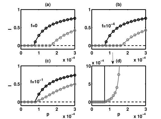
Figure 1: Bifurcation diagram for infected fraction in a static network ($w=0$) as a function of infection rate $p$ for different fractions of cross links $f$. Black: community A; gray: community B. Solid curves: mean field solutions (stable branches); dashed curves: mean field solutions (unstable branches); circles: Monte Carlo simulations. Average degrees $\left<k_{a}\right>\approx 28$ and $\left<k_{b}\right>\approx 12$. The plots correspond to $N_{a}=5\times 10^{3}$, $N_{b}=5\times 10^{3}$, $K=10^{6}$, $d=0.7$ and $r=0.002$. In (d), in order to obtain better statistics, we averaged over 100 network realizations, each of which is similar to (b).

Although a system of two connected communities has an infection threshold at a single bifurcation point, we wish to distinguish between the cases in Figure 1b,c, where significant infection spread occurs in the low degree community (B) if it has sufficient links to the high degree community (A), while the infection in community B is very small if the number of cross links is low. To quantify this, we define effective threshold infection rates $p^{e}_{a}$, $p^{e}_{b}$ for each community as follows. While sweeping the infection rate $p$ from higher to lower values, the first $p$ value at which the fraction of infecteds at the steady state is lower than $\epsilon=10^{-3}$ is considered as the effective threshold infection rate for that community. Figure 2 shows the effective threshold infection rates versus cross link fraction $f$. When $f<10^{-2}$, the effective thresholds in the two communities become noticeably different.

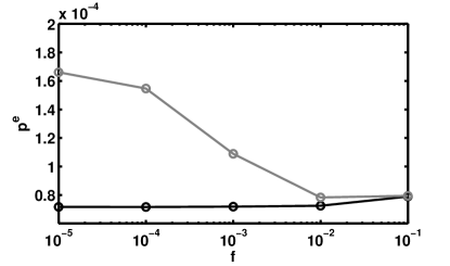
Figure 2: Effective threshold infection rate from mean field vs fraction of cross links $f$. Black curve: community A; gray curve: community B. The infection rate $p$ at which the fraction of infecteds is less than $10^{-3}$ is considered as the effective threshold rate. $N_{a}=5\times 10^{3}$, $N_{b}=5\times 10^{3}$, $K=10^{6}$, $d=0.7$ and $r=0.002$.

III.2 Adaptive network

We now move to systems with nonzero rewiring rates. The bifurcation structure for the adaptive network case was determined as for static networks except for the following modification. In our model, network adaptation does not occur in the absence of infection. This means that the DFS of Equations (1-12) is not isolated, because any disease free combination of AA, AB, and BB links is a steady state. Because of the non-isolated fixed points, the stability of the disease free branch could not be determined using continuation packages. Instead, we calculated numerically the eigenvalues of the Jacobian evaluated at the DFS for the initial network geometry which is described by $f$ and $d$.

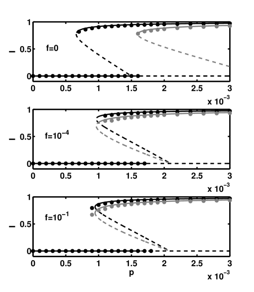
Figure 3: Bifurcation diagram for infected fraction in an adaptive network as a function of infection rate $p$ for different fractions of cross links $f$. Black: community A; gray: community B. Solid curves: mean field solutions (stable branches); dashed curves: mean field solutions (unstable branches); circles: Monte Carlo simulations. Average degrees $\langle k_{a}\rangle\approx 28$ and $\langle k_{b}\rangle\approx 12$. The plots correspond to $N_{a}=5\times 10^{3}$, $N_{b}=5\times 10^{3}$, $K=10^{6}$, $d=0.7$, $w=0.04$ and $r=0.002$. The simulations are done similarly as in Figure 1, but here we run the system for $5\times 10^{6}$ time units in order to approach the endemic branch.

In the absence of community structure ($f=0$), the DFS loses stability at a critical infection rate $p^{*}$, where the unstable endemic branch and the stable disease free branch intersect at a transcritical bifurcation (Figure 3a). The epidemic threshold $p^{*}$ is inversely proportional to the average degree of the network and can be found analytically from the Jacobian of the mean-field equations for a single network (see Appendix).

For a network having two loosely connected heterogenous communities ($f=10^{-4},d=0.7$), $p^{*}$ is very close to that of a single network having the same average degree as community A (Figure 3a,b). This is expected because when the infection in community A starts to spread, a small value of $f$ will not be enough to stop infection spreading in community A. In contrast, for $f=10^{-1}$, $p^{*}$ is larger than that of a single network having the same average degree as community A. In this case, the connection is stronger and the infection starting to spread in community A can be suppressed by the connection to a community where no infection is observed. As we increase $f$, the critical value of $p$ approaches that of a single network with average degree $\langle k\rangle=20$, which is the average degree in the entire system.

In an adaptive network without community structure, bistability can occur for a range of rewiring rates Gross et al. (2006). We focus on the rewiring rate $w=0.04$, for which the endemic branch loses stability at a critical infection rate where the system undergoes a saddle-node (SN) bifurcation. The location of this SN bifurcation depends on the average degree of the network. Figure 3a superimposes the bifurcation diagrams of two single-community networks with different average degrees.

In our model, for a network having two strongly connected communities ($f=10^{-1}$), the endemic state loses stability at a SN bifurcation point. However, for the loosely connected case ($f=10^{-4}$), the endemic branch loses stability at a Hopf bifurcation (HB) point. As with the epidemic threshold (transcritical bifurcation) in static networks, the location of the SN bifurcation and the HB in the adaptive network is governed primarily by the high degree community. However, in contrast with the static case, small cross link fraction $f$ is not associated with low steady state infection levels in the low degree community. As will be seen later in this section, the state with high infection in one community and low in the other community is not a steady state due to the network adaptation. Instead, infection levels are similar in both communities even if weakly connected. Both communities continue to exhibit high infection levels as the number of cross links is further increased (Figure 3c).

By looking at the time series of the mean field equations, we observed a stable periodic solution for a very small range of $p$ values near the HB point. However, we do not see any periodic behavior in the full system due to the narrow range of $p$ values.

As the heterogeneity in the network increases by increasing $d$, the Hopf bifurcation point also increases. Furthermore, the epidemic threshold decreases because of a much higher average degree in community A. This narrows the region where both disease free and endemic branches are stable. In particular, for $d=0.9$, there is no $p$ value where both the endemic steady state and DFS are stable. For $d=0.9$ We observed periodic solutions with a very long period for $p$ values smaller than the HB point in both mean field and the full system.

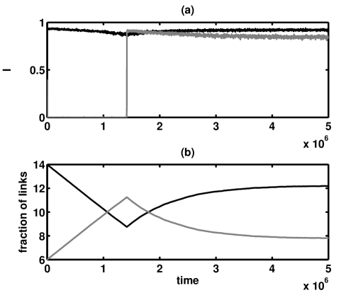
Figure 4: Time series from Monte Carlo simulation of full system. (a) Infected node fractions. Black curve: fraction of infecteds in community A; gray curve: fraction of infecteds in community B. (b) Fraction of links. Black curve: fraction of AA type links; gray curve: fraction of BB type links. Initial condition is as described in the text. $N_{a}=5\times 10^{3}$, $N_{b}=5\times 10^{3}$, $K=10^{6}$, $f=10^{-4}$, $d=0.7$, $w=0.04$, $r=0.002$ and $p=0.0014$.

To motivate the absence of the state seen in static networks with high infection in one community and low infection in the other, we consider a long time series starting initially with a network where $f=10^{-4}$ and $d=0.7$ generated as described above. As seen in Figure 4, the fraction of AA and BB type links change with time. The adaptation rules have been chosen so that if SI links are distributed uniformly throughout the network, the community structure will be preserved. However, with high initial infection levels in A and low in B, there are more SI links among the AA and AB links and fewer among the BB links. This leads to a net flux of link types from AA to AB to BB. (The fraction of AB links (not shown) remains relatively constant at low levels throughout.) Eventually the average degree in the B community exceeds that in the A community and there is an incursion of infection from A to B. The flux of link types is then reversed, and the steady state network structure is similar (but not identical) to that expected from the community structure parameters $d,f$. The infection persists at high levels in both communities at steady state.

We can estimate the time until infection incursion in the B community as follows. From Equations (3,6,10), the fraction of AA links $P_{aa}=P_{SaSa}+P_{SaIa}+P_{IaIa}$ evolves according to

$$\dot{P}_{aa}=w\left[\alpha P_{SaIb}-(1-\alpha)P_{SaIa}\right].$$ (13)

Since we are interested in the critical time when infection starts to spread in community B, we can assume $P_{Ib}\approx 0$ and hence $P_{SaIb}\approx 0$. Thus

$$\dot{P}_{aa} \approx -w(1-\alpha)P_{SaIa}$$ (14)

$$\approx -w(1-\alpha)\gamma P_{aa}$$

where $\gamma=P_{SaIa}/P_{aa}$. Since $f$ is close to zero, we can use the single mean field equations to approximate $\gamma$, the fraction of SI links in community A (see Appendix A). We can then solve Equation (14) for the critical time $t_{c}$ for infection incursion if we know $P_{aa}$ at that time. Since we can predict the critical average degree for community B in order for the disease to spread, we can also find $P_{aa}$ at that point. However, for the full system, the infection in community B starts to spread much earlier than the time found by using mean field equations because of the stochastic nature of our model. Even so, we can solve the equation for $t$ as follows:

$$t = \ln\left[\frac{P_{aa}(0)}{P_{aa}(t)}\right]\left[w(1-\alpha)\gamma\right]^{-1}$$ (15)

from which it can be shown that the critical time $t_{c}$ is proportional to $\frac{1}{f}$. In Figure 5, we can see that the relationship $t_{c}\propto\frac{1}{f}$ holds for the full system.

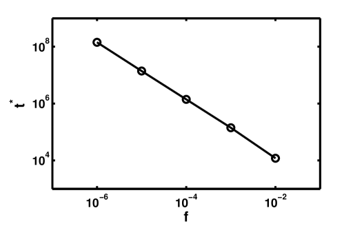
Figure 5: The critical time for infection incursion in community B vs fraction of cross links $f$. The critical time values are averaged over 5 runs except for $f=10^{-6}$. In each run, the time when the fraction of infecteds in community B exceeded $0.1\%$ is considered the critical time.

When the system reaches steady state (late time in Figure 4), the network geometry does not return exactly to that expected from the community structure parameters $f,d$ because the SI links are not uniformly distributed. This effect is most pronounced when the infection rate is below the critical infection rate for the low connectivity network, because then the SI link distribution is the most nonuniform. Figure 6 shows the steady state community structure versus the infection rate. Deviations from the community structure specified by $f,d$ increase as the infection rate approaches the Hopf bifurcation point at $p\approx 0.0019$. Thus the steady state average degree observed in the two communities in the presence of an epidemic can be different than that expected in the absence of an epidemic. The adaptation has a homogenizing effect, bringing the degrees in the communities closer to each other.

For $d=0.9$, the behavior of the system is very interesting. In Fig. 7, we started with similar initial conditions as for $d=0.7$ in Fig. 4. The system behaved similarly for a long time, but once the infection level reached a high value in community B, it could not stay in that state, because a higher $d$ means a higher out flux rate from BB type links. The average degree in B started to decrease, causing infection to die out again in B. A periodic solution with a long period is observed for a range of $p$ values.

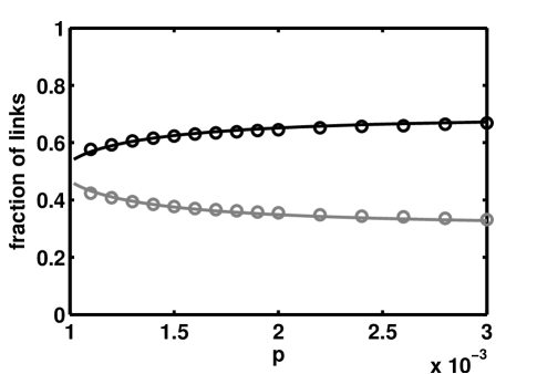
Figure 6: Fraction of links vs infection rate $p$. Curves: mean field steady states; points: Monte Carlo steady state averages. Black: fraction of AA type links; gray: fraction of BB type links. (The fraction of AB links is less than $1\%$.) $N_{a}=5\times 10^{3}$, $N_{b}=5\times 10^{3}$, $K=10^{6}$, $f=10^{-4}$, $d=0.7$, $w=0.04$, $r=0.002$. The data is from the simulations done in Figure 3.

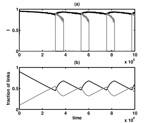
Figure 7: Time series from Monte Carlo simulation of full system. (a) Infected node fractions. Black curve: fraction of infecteds in community A; gray curve: fraction of infecteds in community B. (b) Fraction of links. Black curve: fraction of AA type links; gray curve: fraction of BB type links. Initial condition is as described in the text. $N_{a}=5\times 10^{3}$, $N_{b}=5\times 10^{3}$, $K=10^{6}$, $f=10^{-4}$, $d=0.9$, $w=0.04$, $r=0.002$ and $p=0.0014$.

IV Conclusions

We have studied epidemic spread in a network of two communities with different average degrees. Cases with and without disease avoidance rewiring were considered. Rewiring rules were chosen so that the community structure would be preserved if links between susceptibles and infectives occurred uniformly throughout the network. The steady state bifurcation structure was obtained for static and adaptive cases. A mean field theory based on a moment closure approximation accurately predicted the steady state infection levels and network structure observed in stochastic simulations of the full model.

In the static network case, weakly connected communities displayed significantly different infection levels. Low infection levels could persist in a subthreshold community weakly connected to a high degree, high infection community. Increasing the number of connections between communities led to more similar behavior of the two communities. In contrast, communities in adaptive networks displayed similar infection levels even if weakly connected. Steady states with high infection in one community and low in the other did not exist for the adaptive network case.

The absence of steady states with significantly different infection levels was explained by considering network adaptation in the presence of nonuniformly distributed SI links. If one community has few infectives, there is a net flux of links into that community until its degree is high enough to support the infection. We estimated the time until this infection incursion based on mean field arguments and found that the time increases as the number of cross links between communities decreases.

We also observed changes in the steady state network geometry due to adaptation in the presence of infection. These changes were most significant near bifurcation points. The adaptation tended to bring the average degrees of the communities closer to each other. Thus the adaptation promotes greater similarity between communities in both network structure and infection levels.

The model presented in this paper is the first to include community structure in epidemic spread on an adaptive network. Future work is needed to extend the model to more realistic scenarios. For example, the number of communities could be increased beyond two. We have observed that the convergence time to steady state can be very long for weakly coupled communities, so it is possible that an epidemic would not reach steady state during physically realistic time scales. Thus the transient behavior should also be studied in more detail. Identifying when communities become at risk for incursion of infection could be valuable in knowing when epidemic control measures are needed. Another area for future extension is to change the rules for adaptation, such as cutting or temporarily deactivating links rather than rewiring them.

This work was supported by the Army Research Office, Air Force Office of Scientific Research, and by Award Number R01GM090204 from the National Institute Of General Medical Sciences. The content is solely the responsibility of the authors and does not necessarily represent the official views of the National Institute of General Medical Sciences or the National Institutes of Health.

Appendix A Analytical solution for a single community

For a single community ($f=0$), the mean field equations are:

$$\dot{P}_{I} = -rP_{I}+\frac{pK}{N}P_{SI}$$

$$\dot{P}_{SI} = 2r(1-P_{SI}-P_{SS})-(r+p+w)P_{SI}$$

$$+\frac{2pK}{N}\frac{P_{SS}P_{SI}}{P_{S}}-\frac{pK}{N}\frac{P_{SI}^{2}}{P_{S}}$$

$$\dot{P}_{SS} = rP_{SI}+wP_{SI}$$

$$-\frac{2pK}{N}\frac{P_{SS}P_{SI}}{P_{S}}$$

At steady state, we obtain

$$-rP_{I}+\frac{pK}{N}P_{SI}=0$$ (17)

$$2r(1-P_{SI}-P_{SS})-(r+p+w)P_{SI}$$

$$+\frac{2pK}{N}\frac{P_{SS}P_{SI}}{P_{S}}-\frac{pK}{N}\frac{P_{SI}^{2}}{P_{S}}=0$$ (18)

$$rP_{SI}+wP_{SI}-\frac{2pK}{N}\frac{P_{SS}P_{SI}}{P_{S}}=0$$ (19)

To find the endemic steady state, we first solve [17] for $P_{SI}$, and substitute into [18]. Then we solve [18] for $P_{SS}$ in terms of $P_{I}$. After substituting that into [19], we obtain a quadratic equation in $P_{I}$, $AP_{I}^{2}+BP_{I}+C=0$, where

$$A = p-w$$

$$B = 2w-p-2p\frac{K}{N}$$

$$C = 2p\frac{K}{N}-w-r$$

The quadratic can be solved analytically for $P_{I}$, and then $P_{SI}$ and the other link variables can be computed.

References

- Albert and Barabási (2002) R. Albert and A.-l. Barabási, Reviews of Modern Physics 74 (2002).
- Dorogovtsev and Mendes (2002) S. N. Dorogovtsev and J. Mendes, Advances in Physics 51, 1079 (2002).
- Newman (2003) M. Newman, SIAM review 45, 167 (2003).
- Pastor-Satorras and Vespignani (2001a) R. Pastor-Satorras and A. Vespignani, Physical Review E 63, 066117 (2001a).
- Kuperman and Abramson (2001) M. Kuperman and G. Abramson, Physical Review Letters 86, 2909 (2001).
- May (2001) R. May, Physical Review E 64, 066112 (2001).
- Pastor-Satorras and Vespignani (2001b) R. Pastor-Satorras and A. Vespignani, Physical review letters 86, 3200 (2001b).
- Newman (2002) M. Newman, Physical Review E 66, 016128 (2002).
- Gross et al. (2006) T. Gross, C. D’Lima, and B. Blasius, Physical review letters 96, 208701 (2006).
- Schwartz and Shaw (2010) I. Schwartz and L. Shaw, Physics 3, 17 (2010).
- Gross and Blasius (2008) T. Gross and B. Blasius, Journal of the Royal Society Interface 5, 259 (2008).
- Zanette and Risau-Gusmán (2008) D. Zanette and S. Risau-Gusmán, Journal of biological physics 34, 135 (2008).
- Shaw and Schwartz (2008) L. Shaw and I. Schwartz, Physical Review E 77, 066101 (2008).
- Van Segbroeck et al. (2010) S. Van Segbroeck, F. C. Santos, and J. M. Pacheco, PLoS Computational Biology 6, e1000895 (2010).
- Marceau et al. (2010) V. Marceau, P. Noël, L. Hébert-Dufresne, A. Allard, and L. Dubé, Physical Review E 82, 036116 (2010).
- Newman and Girvan (2004) M. E. J. Newman and M. Girvan, Physical review E 69, 026113 (2004).
- Yan et al. (2007) G. Yan, Z.-Q. Fu, J. Ren, and W.-X. Wang, Physical Review E 75, 1 (2007).
- Huang and Li (2007) W. Huang and C. Li, J.Stat.Mechanics pp. 1–13 (2007).
- Chu et al. (2009) X. Chu, J. Guan, Z. Zhang, and S. Zhou, Journal of Statistical Mechanics: Theory and Experiment 2009, P07043 (2009).
- Zhao and Gao (2007) H. Zhao and Z. Y. Gao, Europhysics Letters (EPL) 79, 38002 (2007).
- Liu (2005) Z. Liu, EPL (Europhysics Letters) 72, 315 (2005).
- Zhou and Liu (2009) J. Zhou and Z. Liu, Physica A: Statistical Mechanics and its Applications 388, 1228 (2009).
- Xia et al. (2009) C. Xia, S. Sun, F. Rao, J. Sun, J. Wang, and Z. Chen, Frontiers of Computer Science in China 3, 361 (2009).
- Sun and Gao (2007) H. Sun and Z. Gao, Physica A: Statistical Mechanics and its Applications 381, 491 (2007).
- Wang et al. (2011) B. Wang, L. Cao, H. Suzuki, and K. Aihara, Journal of Physics A: Mathematical and Theoretical 44, 035101 (2011).
- T and Gillespie (1976) D. T and Gillespie, Journal of Computational Physics 22, 403 (1976).
- Ermentrout (2002) B. Ermentrout, Simulating, Analyzing, and Animating Dynamical Systems A Guide to XPPAUT for Researchers and Students 1st ed. Philadelphia, PA: Soc. Industrial Appl. Math. (2002).