Sparsely Sampling the Sky: A Bayesian Experimental Design Approach

Abstract

The next generation of galaxy surveys will observe millions of galaxies over large volumes of the universe. These surveys are expensive both in time and cost, raising questions regarding the optimal investment of this time and money. In this work we investigate criteria for selecting amongst observing strategies for constraining the galaxy power spectrum and a set of cosmological parameters. Depending on the parameters of interest, it may be more efficient to observe a larger, but sparsely sampled, area of sky instead of a smaller contiguous area. In this work, by making use of the principles of Bayesian Experimental Design, we will investigate the advantages and disadvantages of the sparse sampling of the sky and discuss the circumstances in which a sparse survey is indeed the most efficient strategy. For the Dark Energy Survey (DES), we find that by sparsely observing the same area in a smaller amount of time, we only increase the errors on the parameters by a maximum of 0.45%. Conversely, investing the same amount of time as the original DES to observe a sparser but larger area of sky we can in fact constrain the parameters with errors reduced by 28%.

1 Introduction

The measurements of the cosmological parameters heavily rely on accurate measurements of power spectra. Power spectra describe the spatial distribution of an isotropic random field, defined as the Fourier transform of the spatial correlation function. The perturbations in the universe can be described statistically using the correlation function $\xi(r)$ between two points, which depends only on their separation $r$ (when isotropy is assumed);

$$\xi(r)\equiv\left\langle\delta(\underline{x})\delta(\underline{x}+\underline{r})\right\rangle\;,$$ (1)

where $\delta(\underline{x})=\left(\rho(\underline{x})-\bar{\rho}\right)/\bar{\rho}$ measures the continuous over-density, where $\rho(\underline{x})$ is the density at position $\underline{x}$ and $\bar{\rho}$ is the average density. The power spectrum $P(k)$, which is the Fourier transform of the correlation function, is enough to define the perturbations completely when the perturbations are assumed uncorrelated Gaussian random fields in the Fourier space. Power spectra (or correlation functions) are what the surveys actually measure, from which cosmological parameters are inferred. These spectra are normally a convolution of the primordial power spectrum (which measures the statistical distribution of perturbations in the early universe) and a transfer function which depends on the cosmological parameters. Hence accurate measurements of the power spectra from surveys are very important for accurate measurements of the cosmological parameters.

The most important observed spatial power spectrum for cosmology is the galaxy power spectrum; the Fourier transform of the galaxy correlation function, which was first formulated by Peebles (1973). A galaxy survey lists the measured positions of the observed galaxies. As proposed by Peebles, these positions are modelled as a random Poissonian point source, where the galaxy density is modulated by the fluctuations in the underlying matter distribution and the selection effects. The selection function of the survey is described by $\bar{n}(\underline{x})$, which is the expected galaxy density at position $\underline{x}$ in the absence of clustering. The fluctuations in the underlying matter density are given by $\delta(\underline{x})$, as described previously. The the galaxy number over-density $n(\underline{x})$, which is the observed quantity, is related to the matter over-density via the bias $b$ (Kaiser, 1984) — galaxies trace dark matter up to this $b$ factor. We define the galaxy power spectrum $P_{g}(k)$ as

$$P_{g}(k)=2\pi^{2}\cdot b^{2}(k)\cdot k\cdot T^{2}(k)\cdot P_{p}(k)\;,$$ (2)

where $P_{p}(k)$ is the primordial power spectrum $P_{p}(k)=A_{s}k^{n_{s}-1}$. The transfer function $T(k)$ further depends upon the cosmological parameters (e.g., the matter density $\Omega_{m}$, the scalar spectral index, $n_{s}$, etc.) responsible for the evolution of the universe. The bias $b$ relates the galaxy power spectrum to the matter power spectrum, as explained above.

This power spectrum is very rich in terms of constraining a large range of cosmological parameters. On large scales this spectrum probes structure which is less affected by clustering and evolution. Hence these scales are still in the linear regime and have a “memory” of the initial state. The information from these regimes are, therefore, the cleanest since the Big Bang and any knowledge on these large scales would shed light on the physics of early universe and hence the primordial power spectrum. On intermediate scales the spectrum provides us with information about the evolution of the universe since the Big Bang; for example the matter-radiation equality which is responsible for the peak of the galaxy spectrum. The matter-radiation equality is a unique point in the history of the evolution, giving information about the amount of matter and radiation in the universe. On relatively small scales there is a great deal of information about galaxy clustering via the Baryonic Acoustic Oscillations (BAO) which encode a characteristic scale; the sound horizon at the time of recombination. Therefore, measuring the galaxy power spectrum on a large range of scales can help us constrain the cosmological parameters responsible for the evolution of the universe as well as the ones of its initial state.

Accurate measurements of the galaxy power spectrum depend on two main factors; the Poisson noise and the cosmic variance. To overcome the Poisson noise, surveys aim to maximise the number of galaxies observed. The impressive constraints on cosmological parameters from previous and current surveys, such as the 2dF (Croom et al., 2004) and SDSS (Adelman-McCarthy et al., 2008), has motivated even more ambitious future surveys such as DES (The Dark Energy Survey Collaboration, 2005) and Euclid (Laureijs, 2009), aiming to observe millions of galaxies over large volumes of the universe. Considering the large investments in time and money for these surveys, one wants to ask what is really the optimal survey strategy! In this work we want to investigate this exact questions and find the optimal strategy for galaxy surveys such as DES and Euclid.

In this era of cosmology where the statistical errors have reduced greatly and are now comparable with systematics, observing, for example, a greater number of galaxies may not necessarily improve our results. We need to devise more strategic ways to make our observations and take control of our systematics. For example, to investigate larger scales, it may be more efficient to observe a larger, but sparsely sampled, area of sky instead of a smaller contiguous area. In this case we would gather a larger density of states in Fourier space, but at the expense of an increased correlation between different scales — aliasing. This would smooth out features on these scales and decrease its significance if any observed. Here, by making use of Bayesian Experimental Design we will investigate the advantages and disadvantages of the sparse sampling and verify if a complete contiguous survey is indeed the most efficient way of observing the sky for our purposes. The parameter of interest here is the galaxy power spectrum itself and a set of cosmological parameters that depend on this spectrum.

Some previous work on sparse sampling includes Kaiser (1986) and Blake et al. (2006); Kaiser (1986) shows that measuring the large scale correlation function from a complete magnitude-limited redshift survey is actually not the most efficient approach. Instead, sampling a fraction of galaxies randomly, but to a fainter magnitude limit, will improve the constraints of the correlation function measurements significantly, for the same amount of observing time. Blake et al. (2006) have shown that a sparse-sampling (achieved by a non-contiguous telescope pointings or, for a wide-field multi-object spectrograph, by having the fibres distributed randomly across the field-of-view) is preferred when the angular size of the sparse observed patches is much smaller than angular scale of the features in the power spectrum (the acoustic features).

2 Bayesian Experimental Design and Figure-of-Merit

Bayesian methods have recently been used in cosmology for model comparison and for deriving posterior probability distributions for parameters of different models. However, Bayesian statistics can do even more by handling questions about the performance of future experiments, based on our current knowledge (Liddle et al., 2006; Trotta, 2007a, b). For example, Parkinson et al. (2007) use a Bayesian approach to constrain the dark energy parameters by optimising the Baryon Acoustic Oscillations (BAO) surveys. By searching through a survey parameter space (which includes parameters such as redshift range, number of redshift bins, survey area, observing time, etc.) they find the optimal survey with respect to the dark energy equation-of-state parameters. Here we will use this strength of Bayesian statistics for optimising the strategy to observe the sky for galaxy surveys. There are three requirements for such an optimisation; 1. specify the parameters that define the experiment which need to be optimised for an optimal survey; 2. specify the parameters to constrain, with respect to which the survey is optimised; 3. specify a quantity of interest, generally called the figure of merit (FoM), associated with the proposed experiment. The choice of the FoM depends on the questions being asked, as will be explained later in the text. We then want to extrimise the FoM subject to constraints imposed by the experiment or by our knowledge about the nature of the universe. Below, we will explain the procedure.

Assume $e$ denotes the different experimental designs that we can implement and $M^{i}$ are the different models under consideration with their parameters $\theta^{i}$. Assume that experiment $o$ has been performed, so that this experiment’s posterior $P(\theta|o)$ forms our prior probability function for the new experiment. The FoM will depend on the set of parameters under investigation, the performed experiment (data) and the characteristics of the future experiment; $U(\theta,e,o)$. From the utility we can build the expected utility $E\left[U\right]$ as

$$E[U|e,o]=\sum_{i}P(M^{i}|o)\int d\hat{\theta}^{i}\;U(\hat{\theta}^{i},e,o)P(\hat{\theta}^{i}|o,M^{i})\>,$$ (3)

where $\hat{\theta}^{i}$ represent the fiducial parameters for model $M^{i}$. This says: If a set of fiducial parameters, $\hat{\theta}$, correctly describe the universe and we perform an experiment $e$, then we can compute the utility function for that experiment, $U(\hat{\theta},e,o)$. However, our knowledge of the universe is described by the current posterior distribution $P(\hat{\theta}|o)$. Averaging the utility over the posterior accounts for the present uncertainty in the parameters and summing over all the available models would account for the uncertainty in the underlying true model. The aim is to select an experiment that extremises the utility function (or its expectation). The utility function takes into account the current models and the uncertainties in their parameters and, therefore, extremising it takes into account the lack of knowledge of the true model of the universe.

One of the common choices for the FoM is some form of function of the Fisher matrix, which is the expectation of the inverse covariance of the parameters in the Gaussian limits (We will explain in the next section how a Fisher matrix is obtained in more detail.). One can refer to the Dark Energy Task Force (DETF) FoM, that use Fisher-matrix techniques to investigate how well each model experiment would be able to restrict the dark energy parameters $w_{0}$, $w_{a}$, $\Omega_{DE}$ for their purposes. Three common FoMs, which we will be using as well, are

• A-optimality $=\log(\textrm{trace}(\mathbf{F}))$
  trace of the Fisher matrix (or its $\log$) and is proportional to sum of the variances. This prefers a spherical error region, but may not necessarily select the smallest volume.

• D-optimality $=\log\left(\left|\mathbf{F}\right|\right)$
  determinant of the Fisher matrix (or its $\log$), which measures the inverse of the square of the parameter volume enclosed by the posterior. This is a good indicator of the overall size of the error over all parameter space, but is not sensitive to any degeneracies amongst the parameters.

• Entropy (also called the Kullback-Leibler divergence)

  $$E = \int d\theta\;P(\theta|\hat{\theta},e,o)\log\frac{P(\theta|\hat{\theta},e,o)}{P(\theta|o)}$$ (4)

  $$= \frac{1}{2}\left[\log\left|\mathbf{F}\right|-\log|\mathbf{\Pi}|-\textrm{trace}(\mathbb{I}-\mathbf{\Pi}\mathbf{F}^{-1})\right]\,,$$

  where $P(\theta|\hat{\theta},e,o)$ is the posterior distribution with Fisher matrix $\mathbf{F}$ and $P(\theta|o)$ is the prior distribution with Fisher matrix $\mathbf{\Pi}$. The entropy forms a nice compromise between the A-optimality and D-optimality. Note that these are the utility functions, not the ‘expected’ utility functions. In our current models of the universe, we do not expect a significant difference between the parameters of the same model. However, this will be investigated in a future work, where we will explicitly use expected utility functions. In the next section we will explain how a Fisher matrix is formulated.

3 Fisher Matrix Analysis

The Fisher matrix is generally used to determine the sensitivity of a particular survey to a set of parameters and has been largely used for optimisation (and forecasting). Consider the likelihood function for a future experiment with experimental parameters $e$, $\mathcal{L}(\theta|e)\equiv P(D_{\hat{\theta}}|\theta,e)$, where $D_{\hat{\theta}}$ are simulated data from the future experiment assuming that $\hat{\theta}$ are the true parameters in the given model. We Taylor expand the log-likelihood around its maximum value:

$$\ln\mathcal{L}(\theta|e)=\ln\mathcal{L}(\theta^{ML})+\frac{1}{2}\sum_{ij}(\theta_{i}-\theta_{i}^{ML})\frac{\partial^{2}\ln\mathcal{L}}{\partial\theta_{i}\partial\theta_{j}}(\theta_{j}-\theta_{j}^{ML})\>,$$ (5)

where the first term is a constant and only affects the height of the function, the second term describes how fast the likelihood function falls around the maximum. The Fisher matrix is defined as the ensemble average of the curvature of the likelihood function $\mathcal{L}$ (i.e., it is the average of the curvature over many realisations of signal and noise);

$$F_{ij} = \left\langle\mathcal{F}\right\rangle=\left\langle-\frac{\partial^{2}\ln\mathcal{L}}{\partial\theta_{i}\partial\theta_{j}}\right\rangle$$ (6)

$$= \frac{1}{2}\textrm{trace}[C_{,i}C^{-1}C_{,j}C^{-1}]\>,$$ (7)

where the second line is appropriate for a Gaussian distribution with correlation matrix $C$ determined by the parameters $\theta_{i}$, and $\mathcal{L}$ is the likelihood function. The inverse of the Fisher matrix is an approximation of the covariance matrix of the parameters, by analogy with a Gaussian distribution in the $\theta_{i}$, for which this would be exact. The Cramer-Rao inequality states that the smallest frequentist error measured, for $\theta_{i}$, by any unbiased estimator (such as the maximum likelihood) is $1/\sqrt{F_{ii}}$ and $\sqrt{(F^{-1})_{ii}}$, for non-marginalised and marginalised one-sigma errors respectively. The derivatives in Equation 6 generally depend on where in the parameter space they are calculated and hence it is clear that the Fisher matrix is function of the fiducial parameters.

The Fisher matrix allows us to estimate the errors on parameters without having to cover the whole parameter space (but of course will only be appropriate so long as the derivatives are roughly constant throughout the space). So, a Fisher matrix analysis is equivalent to the assumption of a Gaussian distribution about the peak of the likelihood (e.g. Bond et al., 1998). It also makes the calculations easier. For example, if we are only interested in a subset of parameters, then marginalising over unwanted parameters is just the same as inverting the Fisher matrix, taking only the rows and columns of the wanted parameters and inverting the smaller matrix back. It is also very straightforward to combine constraints from different independent parameters: we just sum over the Fisher matrices of the experiments (remember Fisher matrix is the $\log$ of the likelihood function).

We further note, as in all uses of the Fisher matrix, that any results thus obtained must be taken with the caveat that these relations only map onto realistic error bars in the case of a Gaussian distribution, usually most appropriate in the limit of high signal-to-noise ratio and/or relatively small scales, so that the conditions of the central limit theorem obtain. As long as we do not find extremely degenerate parameter directions, we expect that our results will certainly be indicative of a full analysis, using simulations and techniques such as Bayesian Experimental Design (Trotta, 2007c).

3.1 Fisher Matrix for Galaxy Surveys

We follow the approach of Tegmark (1997) to define the pixelisation for galaxy surveys. First we define the data in pixel $i$ as

$$\Delta_{i}\equiv\int d^{3}x\psi_{i}\left(\underline{x}\right)\left[\frac{n\left(\underline{x}\right)-\bar{n}}{\bar{n}}\right]\,,$$ (8)

where $n(\underline{x})$ is the galaxy density at position $\underline{x}$ and $\bar{n}$ is the expected number of galaxies at that position. The weighting function, $\psi_{i}(\underline{x})$, which determines the pixelisation (and is sensitive to the shape of the survey as you will see later), is defined as a set of Fourier pixels

$$\psi_{i}(\underline{x})=\frac{e^{\iota\underline{k}_{i}.\underline{x}}}{V}\times\begin{cases}1&\,\vec{x}\,\,\textnormal{ inside\,\,\ survey\,\,\ volume}\\ 0&\,\textnormal{otherwise}\end{cases}\,,$$ (9)

where $V$ is the volume of the survey. Here we have divided the volume into sub-volumes, each being much smaller than the total volume of the survey, but being large enough to contain many galaxies. This means $\Delta_{i}$ is the fractional over-density in pixel $i$. Using this pixelisation we can define a covariance matrix as

$$\left\langle\Delta_{i}\Delta_{j}^{*}\right\rangle=C=(C_{S})_{ij}+(C_{N})_{ij}\,,$$ (10)

where $C_{S}$ and $C_{N}$ are the signal and noise covariance matrices respectively and are assumed independent of each other. The signal covariance matrix can be defined as

$$(C_{S})_{ij} = \left\langle\Delta_{i}\Delta_{j}^{*}\right\rangle$$ (11)

$$= \int d^{3}xd^{3}x^{\prime}\;\psi_{i}(\underline{x})\psi_{j}^{*}(\underline{x}^{\prime})$$

$$\left\langle\frac{n(\underline{x})-\bar{n}}{\bar{n}}\cdot\frac{n(\underline{x}^{\prime})-\bar{n}}{\bar{n}}\right\rangle\,.$$

By equating the number over-density $\left(n(\underline{x})-\bar{n}\right)/\bar{n}$ to the continuous over-density $\delta(\underline{x})=\left(\rho(\underline{x})-\bar{\rho}\right)/\bar{\rho}$ we obtain

$$(C_{S})_{ij} = \int\frac{d^{3}k}{(2\pi)^{3}}P(k)\tilde{\psi}_{i}(\underline{k})\tilde{\psi}_{j}^{*}(\underline{k})$$ (12)

$$= \int\frac{dk}{(2\pi)^{3}}k^{2}P(k)\int d\Omega_{k}\;\tilde{\psi}_{i}(\underline{k})\tilde{\psi}_{j}^{*}(\underline{k})$$

$$= \int\frac{dk}{(2\pi)^{3}}k^{2}P(k)W_{ij}(k)\,,$$

where $\tilde{\psi}_{i}(\underline{k})$ is the Fourier transform of $\psi_{i}(\underline{x})$ and the window function $W_{ij}(k)$ is defined as the angular average of the square of the Fourier transform of the weighting function. With the same approach, the noise covariance matrix — which is due to Poisson shot noise — is given by

$$(C_{N})_{ij} = \left\langle N_{i}N_{j}^{*}\right\rangle_{\textnormal{Noise}}$$ (13)

$$= \int d^{3}xd^{3}x^{\prime}\psi_{i}\left(\underline{x}\right)\psi_{j}^{*}\left(\underline{x}^{\prime}\right)\frac{1}{\overline{n}}\delta_{D}\left(\underline{x}-\underline{x}^{\prime}\right)$$

$$= \int\frac{d^{3}k}{(2\pi)^{3}}\frac{1}{\overline{n}}\tilde{\psi}_{i}(\underline{k})\tilde{\psi}_{j}^{*}(\underline{k})$$

$$= \int\frac{dk}{(2\pi)^{3}}k^{2}\frac{1}{\overline{n}}\int d\Omega_{k}\tilde{\psi}_{i}(\underline{k})\tilde{\psi}_{j}^{*}(\underline{k})$$

$$= \frac{1}{\overline{n}}\int\frac{dk}{(2\pi)^{3}}k^{2}W_{ij}(k)\ .$$

The design of the survey will shape the form of the weighting function in Equation 9, which will be discussed in the next section.

This prescription gives us a data covariance matrix for a galaxy survey. What we actually need is a Fisher matrix for the parameters we are interested in. For this we will use Equation 6 above, which defines the Fisher matrix of parameters in terms of the inverse of the data covariance matrix and its differentiation with respect to the parameters of interest. We are interested in the galaxy power spectrum and hence the differentiation of the covariance matrix in Equation 6 is taken with respect to the bins of this power spectrum. As the noise covariance matrix does not depend on the power spectrum, we only need to differentiate the signal covariance matrix in Equation 12. Taking the galaxy power spectrum as a series of top-hat bins

$$P(k)=\sum_{B}w_{B}(k)P_{B}\quad\begin{cases}w_{B}=1&\,\,k\in B\\ 0&\,\textnormal{otherwise}\end{cases}\,,$$ (14)

where $P_{B}$ is the power in each bin, the differentiation takes the form

$$\frac{\partial(C_{S})_{ij}}{\partial P(k)}=\int_{k_{B}^{min}}^{k_{B}^{max}}\frac{dk}{(2\pi)^{3}}k^{2}W_{ij}(k)\,.$$ (15)

We insert this and the inverse of the data covariance matrix into Equation 6 to get a Fisher matrix for the galaxy power spectrum bins. To get a Fisher matrix for the cosmological parameters one can use the parameters Jacobian

$$F_{\alpha\beta}=\sum_{ab}F_{ab}\frac{\partial P_{a}}{\partial\lambda_{\alpha}}\frac{\partial P_{b}}{\partial\lambda_{\beta}}\;.$$ (16)

where $F_{ab}$ is the galaxy spectrum Fisher matrix and $F_{\alpha\beta}$ is the Fisher matrix for the cosmological parameters $\lambda_{\alpha}$ and $\lambda_{\beta}$.

4 Survey Design

We will investigate the FoM of a sparse design to that of a contiguous survey, which we have chosen to be similar to that of the Dark Energy Survey (DES).

4.1 Dark Energy Survey (DES)

The Dark Energy Survey (DES) (The Dark Energy Survey Collaboration, 2005) is designed to probe the origin of the accelerating universe and help uncover the nature of dark energy. Its digital camera, DECam, is mounted on the Blanco 4-meter telescope at Cerro Tololo Inter-American Observatory in the Chilean Andes. Starting in December 2012 and continuing for five years, DES will catalogue 300 million galaxies in the southern sky over an area of 5000 square degrees and a redshift range of $0.2<z<1.3$. In the next section we will explain how we ‘sparsify’ the DES survey for our purposes.

Here, we use a flat-sky approximation. Euclid, with a survey area of $20,000$ square degrees should be treated on the full sky and is not investigated here. Nonetheless we expect qualitatively similar results to DES.

4.2 Sparse Design

Figure 1: Design of the mask on the sky to sparsely sample the sky. A regular grid with $n$ patches of size $M$ (note that we are observing through these patches — white squares in the Figure), placed at constant distances from one another at $x_{i}$ and $y_{j}$. The total observed area is the sum of the areas of all the patches, $n\times M^{2}$, and total sampled area is the total area which bounds both the masked and the unmasked areas, $V$. Hence the fraction of sky observed is $f=(n\times M^{2})/A_{\textrm{tot}}$. Also, note that we are assuming a flat-sky approximation.

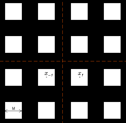
For simplicity, we will design the sparsely sampled area of the sky as a regular grid of $n_{p}\times n_{p}$ square patches of size $M\times M$ — Figure 1. We therefore define the structure on the sky as a top-hat in both $x$ and $y$ directions

$$\sum_{n}\Pi(x-x_{n}) = \begin{cases}1&\,0<|x-x_{n}|<M/2\\ 0&\,\textnormal{otherwise}\end{cases}\,,$$ (17)

$$\sum_{m}\Pi(y-y_{m}) = \begin{cases}1&\,0<|y-y_{m}|<M/2\\ 0&\,\textnormal{otherwise}\end{cases}\,,$$ (18)

where $x_{i}$ and $y_{j}$ mark the centres of the patches in our coordinate system. In the $z$ direction we use the step function, which is defined as:

$$\Theta(z) = \begin{cases}1&z>0\\ 0&\,\textnormal{otherwise}\end{cases}\,.$$ (19)

With this design the weight function in equation 9 takes the form:

$$\tilde{\psi}_{i}(\underline{k}) = \int d^{3}x\;e^{\imath(\underline{k}_{i}-\underline{k}).\underline{x}}\;\;\;\times\;$$ (20)

$$\;\;\;\;\sum_{n}\Pi(x-x_{n})\sum_{m}\Pi(y-y_{m})\;\;\;\times\;$$

$$\;\;\;\;\Theta\left(z+\frac{L}{2}\right)\Theta\left(\frac{L}{2}-z\right)\;\times\frac{1}{V}$$

$$= \int dxe^{\imath q_{x}x}\sum_{n}\Pi(x-x_{n})\;\;\;\times\;$$

$$\int dye^{\imath q_{y}y}\sum_{m}\Pi(y-y_{m})\;\;\;\times\;$$

$$\int dze^{\imath q_{z}z}\Theta\left(z+\frac{L}{2}\right)\Theta\left(\frac{L}{2}-z\right)\;\times\frac{1}{V}$$

$$= \text{sinc}\left(q_{x}\frac{M}{2}\right)\sum_{n}2\cos\left(q_{x}x_{n}\right)\;\;\;\times\;$$

$$\text{sinc}\left(q_{y}\frac{M}{2}\right)\sum_{m}2\cos\left(q_{y}y_{m}\right)\;\;\;\times\;$$

$$\text{sinc}\left(q_{z}\frac{L}{2}\right)\;\times\frac{M^{2}L}{V}\ ,$$

where $\underline{q}=\underline{k}_{i}-\underline{k}$, $q_{x}=q\sin\theta\cos\phi$, $q_{y}=q\sin\theta\sin\phi$, $q_{z}=q\cos\phi$ and $d\mu=d\cos\theta$. The volume $V$ is the total sparsely sampled volume, $M$ is the size of the observed patch on the surface of the sky and $L$ is the observed depth. The last equality in the above equation uses the Dirichlet Kernel

$$D_{n}(x)=\sum_{k=-n}^{n}e^{ikx}=1+2\sum_{k=1}^{n}\cos(kx)\,,$$ (21)

which can be used due to the symmetry of the design. The window function, defined in Equation 12, now takes the form

$$W_{ij}(k) = \int_{-1}^{1}\frac{d\mu}{2}\int_{0}^{2\pi}\frac{d\phi}{2\pi}\tilde{\psi}(\underline{k}_{i}-\underline{k})\tilde{\psi^{*}}(\underline{k}_{j}-\underline{k})$$ (22)

$$= \int_{-1}^{1}\frac{d\mu}{2}\int_{0}^{2\pi}\frac{d\phi}{2\pi}\times\left(\frac{M^{2}L}{V}\right)^{2}\times$$

$$\;\;\;\;\;\;\;\text{sinc}\left(q_{x}\frac{M}{2}\right)\sum_{n}2\cos(q_{x}x_{n})\times$$

$$\;\;\;\;\;\;\;\text{sinc}\left(q_{x}^{\prime}\frac{M}{2}\right)\sum_{n^{\prime}}2\cos(q_{x}^{\prime}x_{n^{\prime}})\times$$

$$\;\;\;\;\;\;\;\text{sinc}\left(q_{y}\frac{M}{2}\right)\sum_{m}2\cos(qy_{m})\times$$

$$\;\;\;\;\;\;\;\text{sinc}\left(q_{y}^{\prime}\frac{M}{2}\right)\sum_{m^{\prime}}2\cos(q_{y}^{\prime}y_{m^{\prime}})\times$$

$$\;\;\;\;\;\;\;\text{sinc}\left(q_{z}\frac{L}{2}\right)\text{sinc}\left(q_{z}^{\prime}\frac{L}{2}\right)\;.$$

Note that there are two scales that control the behaviour of the window function; one is the size of the patches, $M$, and the other is their distance from one another, $x_{i}$. We will investigate the influence of both of these scales on the FoM by trying two different configurations, discussed in the next section. In case of the contiguous sampling of the sky where we are observing through a contiguous square, the window function takes the form of one single big patch, as shown below

$$W_{ij}(k) = \int_{-1}^{1}\frac{d\mu}{2}\int_{0}^{2\pi}\frac{d\phi}{2\pi}\times$$ (23)

$$\;\;\;\;\;\;\;\text{sinc}\left(q_{x}\frac{M}{2}\right)\text{sinc}\left(q_{x}^{\prime}\frac{M}{2}\right)\times$$

$$\;\;\;\;\;\;\;\text{sinc}\left(q_{y}\frac{M}{2}\right)\text{sinc}\left(q_{y}^{\prime}\frac{M}{2}\right)\times$$

$$\;\;\;\;\;\;\;\text{sinc}\left(q_{z}\frac{L}{2}\right)\text{sinc}\left(q_{z}^{\prime}\frac{L}{2}\right)\;.$$

which is a square cylinder.

4.3 Sparsifying DES

We divide the total area of DES into small square patches, as explained in the design of the mask previously. There are two ways to sparsify this area;

• Constant Total Area (full sampled area stays constant)
  In this setting we keep the patches at a constant position and gradually decrease their size. Therefore, the total sampled area is kept constant, while the total observed area decreases as the patch sizes decrease. The patches are placed at $60\textnormal{Mpc}$ from one another; this scale is about half of the scale of the BAO Scales, which is $\sim 120\textnormal{Mpc}$. The patches are placed at half this scale to capture the BAO features at best. This restricts the maximum size of the patches to be $60\textnormal{Mpc}$ for $f=1$. We then shrink them from $60\textnormal{Mpc}$ to $10\textnormal{Mpc}$. The minimum size of $10\textnormal{Mpc}$ was chosen to avoid entering the non-linear physics at $<10\textnormal{Mpc}$. This configuration is shown in Figure 2. In this case, as we make our observations more sparse, the total observing time decreases as well; we could instead choose to observe more deeply in the same amount of time and gain volume in the redshift direction.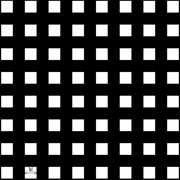

  

  

  

  

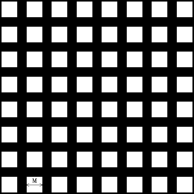
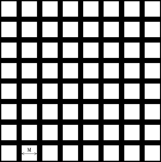
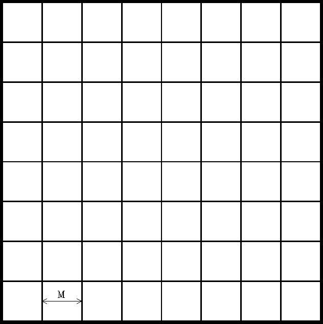
  Figure 2: Survey geometry for the ‘constant total area’ scenario — section 5.1. In this setting we keep the patches at a constant position and gradually decrease their size. Therefore, the total sampled area (i.e., the total extent of the survey) is kept constant, while the total observed area (and hence the survey observing time) decreases as the patch sizes decrease.

• Constant Observed Area (footprint of the survey stays constant)
  In this setting the size of the patches are kept fixed at $60\textnormal{Mpc}$, and the area is sparsified by placing the patches further and further from one another. Here the total observed area is constant, while the total sampled area increases as the patches are put further and further. This configuration is shown in Figure 3. Now, the length of time for the survey remains the same, but is spread out over a larger area of sky.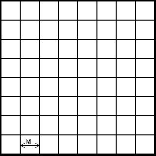
  

  

  

  

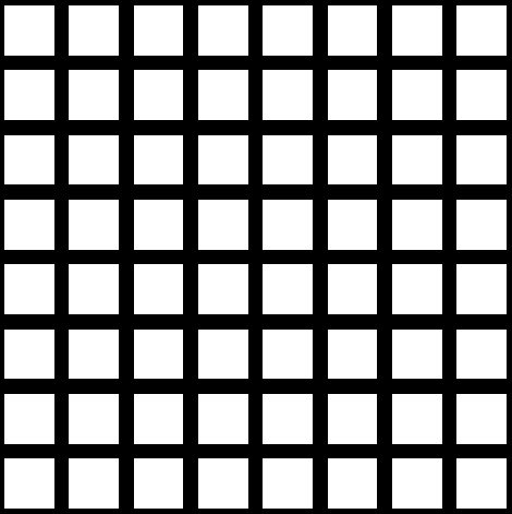
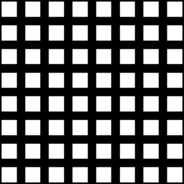
  Figure 3: Survey geometry for the ‘constant observed area’ scenario — section 5.2. In this setting the size of the patches are kept fixed at $60\textnormal{Mpc}$, and the area is sparsified by placing the patches further and further from one another. Here the total observed area (and hence the survey observing time) is constant, while the total sampled area (i.e., the total extent of the survey) increases as the patches are put further and further.

Note that the areas we consider here are small enough that the flat sky approximation is valid. Also note that in all the above setting we keep the number of bins of the galaxy power spectrum constant at $n_{\textrm{bin}}=60$. In reality we should let the total volume of the survey choose the binning of the power spectrum via $k_{min}=(2\pi/V)^{1/3}=dk$, and hence the number of the bins $n_{\textrm{bin}}$. However, if $n_{bin}$ changes from case to case it will be unfair to compare D-optimality and Entropy as they will have different units as $n_{bin}$ changes. To have a fair comparison between the cases we keep $n_{\textrm{bin}}$ constant.

5 Results

We have chosen a geometrically flat $\Lambda$CDM model with adiabatic perturbations. We have a five-parameter model with the following values for the parameters: $\Omega_{m}=0.214$, $\Omega_{b}=0.044$, $\Omega_{\Lambda}=0.742$, $\tau=0.087$ and $h=0.719$, where $H_{0}=100h\textnormal{k}\textnormal{m}^{-1}\textnormal{Mp}\textnormal{c}^{-1}$. The FoM used are

Entropy $$= \left[\ln\left|\mathbf{F}\right|-\ln|\mathbf{\Pi}|-\textrm{trace}(\mathbb{I}-\mathbf{\Pi}\mathbf{F}^{-1})\right]$$ (24)

$$\;\times\;0.5\,,$$

A-optimality $$= \ln(\textrm{trace}(\mathbf{F}))\,,$$ (25)

D-optimality $$= \ln(\left|\mathbf{F}\right|)\,,$$ (26)

where $\mathbf{\Pi}$ is the prior Fisher matrix, which we have chosen to be that for a SDSS-LRG-like survey. The posterior Fisher matrix is $\mathbf{F}=\mathbf{L}+\mathbf{\Pi}$, where $\mathbf{L}$ is the likelihood Fisher matrix, which is the current sparse survey we have designed. The utility functions above are defined so that they need to be maximised for an optimal design.

5.1 Constant Total Area

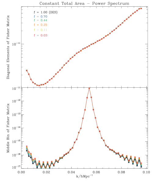
Figures 4 shows the FoM for both the galaxy power spectrum bins on the left and the cosmological parameters on the right. In both cases, the Entropy, A-optimality and D-optimality all increase with $f$. This is as expected as a contiguous sampling of the sky captures all the information and should be the best to constrain cosmology. The top panels in the Figure show A-optimality for the bins on the left and the cosmological parameters on the right. In both cases, $A$ increases with $f$ and reaches its maximum at $f=1$ for DES. Note that A-optimality is a measure of the errors of the parameters only — it is a measure of the trace of the Fisher matrix. Therefore, it is does not account for the correlations between parameters. Although $A$ increases with $f$ for both the bins and the parameters, note that this increase is very small. To see the amount of change in each of the elements of the power spectrum Fisher matrix as $f$ increases, look at the top panel of Figure 5. This shows the diagonal elements of the Fisher matrix $\mathbf{F}$ for galaxy power spectrum bins for the different $f$. The elements are all on top of each other and indeed the gain obtained by increasing $f$ is very small.

The middle panels of Figure 4 show D-optimality, which again increases with $f$ for both the bins and the parameters. Note that, D-optimality is a measure of the determinant of the Fisher matrix and therefore takes the correlation between the parameters into account. The correlation between the parameters is indeed very important; one disadvantage of the sparse sampling is the correlation it induces between the parameters due to aliasing. To see this effect, look at the bottom panel of Figure 5, where the row of the Fisher matrix that corresponds to the middle bin of the power spectrum is shown. Going away from the peak in both direction, the elements show the correlation between the different bins and the middle one. As $f$ decreases and we get more and more sparse, the power in the off-diagonal elements of the Fisher matrix increases, meaning there is more aliasing. The DES survey, as a full contiguous survey, has the least aliasing, while the sparsest survey has the most. The rise towards the small $k$ (large scales) is due to sample variance.

Looking at the correlations and the errors in the Fisher matrix of the spectrum one notes that the decrease in D-optimality for sparser surveys is mostly due to the increased correlation between the bins rather than the the increased errors; as we saw in the top panel of this Figure the decrease in the errors are negligible. In general we conclude that total aliasing induced by sparsity is small and the loss in the constraining power of the survey due to this aliasing is negligible. Hence, overall, little is gained by observing the sky more contiguously.

The bottom panels in Figure 4 show the Entropy for the bins and the parameters. Again, $E$ increases with $f$ and reaches its maximum for DES. The Entropy measures the total size of the errors of the parameters in the Fisher matrix as well as their correlation. Hence it is a good compromise of A- and D-optimality. It measures the total information gain of the survey relative to a prior survey. Having an SDSS-like-survey as our prior, and taking into account both the errors and the correlation between the parameters, the contiguous DES survey has the largest gain compared to the sparse surveys. However, note that this gain is again very small.

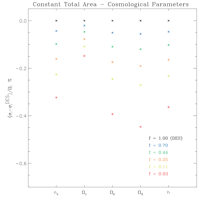
Figure 6 shows the relative loss in the marginalised errors of each of the cosmological parameters with respect to DES. The largest loss for a sparse observation of the sky is on the spectral index with $\delta\Omega_{\Lambda}/\Omega_{\Lambda}\sim 0.45\%$ and the smallest is for $\Omega_{c}$ with a loss of $\delta\Omega_{c}/\Omega_{c}\sim 0.15\%$. The non-marginalised errors show a qualitatively different behaviour, where $n_{s}$ has the largest and $\Omega_{\Lambda}$ has the smallest loss.

Figure 4: ‘Constant total area’ — Figure of Merit for galaxy power spectrum bins on the left and cosmological parameters on the right. In both cases, the Entropy, A-optimality and D-optimality all increase with $f$. This is as expected as a contiguous sampling of the sky captures all the information and should be the best to constrain cosmology. However, note that the increase is indeed very small. In general we conclude that the loss in the constraining power of the survey due to sparsity is negligible and, overall, little is gained by observing the sky more contiguously. Therefore, the sparse surveys seem like a good substitute for the contiguous surveys, with less observing time and less cost.

Figure 5: ‘Constant total area’ — Top panel shows the diagonal elements of the Fisher matrix for different $f$ for the power spectrum bins. The increase in these elements (which translates into a decrease in the variance) is indeed very negligible as sparsity increases. Bottom panel shows the row of the Fisher matrix that corresponds to the middle bin of the power spectrum. Going away from the peak in both direction, these elements show the correlation between the different bins and the middle one. As $f$ decreases and we get more and more sparse, the power in the off-diagonal elements of the Fisher matrix increases, meaning there is more aliasing between the bins. The DES survey, as a full contiguous survey, has the least aliasing, while the sparsest survey has the most aliasing. The uniform increase at low $k$, large scales, is due to sample variance.

Figure 6: ‘Constant total area’ — Relative change in the errors of the cosmological parameters. The largest loss is about $4.5\%$ due to sparsifying the survey.

5.2 Constant Observed Area

Figure 7 shows the FoM for the power spectrum bins and the cosmological parameters. In this case the Entropy, A-optimality and D-optimality all decrease with $f$. And the overall changes in all the FoM are much larger than the ones seen in the previous scenario for both the bins and the parameters.

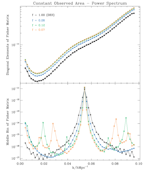
The top panel of Figure 8 shows the diagonal elements of the Fisher matrix of the bins. As we sparsify the survey these elements increase, and hence better constrain the spectrum. The bottom panel in the Figure shows the row of the Fisher matrix that corresponds to the middle bin of the spectrum. Going away from the peak, the elements show the correlation between the different bins and the middle one. For DES the middle bin has a correlation with the close neighbouring bins. However, the correlation decreases as we go away from the peak. Towards small $k$ (large scales) it starts to increase again due to sample variance. As $f$ decreases and we get more and more sparse, the middle bin has a sharper drop (due to the larger total size of the survey) i.e., less correlation with neighbouring bins. However, there is more aliasing between distant bins. Also, there are peaks (i.e., larger correlations) at certain scales which are related to the distances between the patches, which changes case by case. The DES survey, as a full contiguous survey, has indeed the least aliasing, while the sparsest survey has the most.

Note that in this case the sparsity is obtained by placing the observed patches further and further away from each other. As the sparsity increases as the patches are placed further, the total size of the survey is greatly increased, which seems to make up for the aliasing that the sparse design has induced. Overall we gain a great deal by spending the same amount of time on larger but sparsely sampled area.

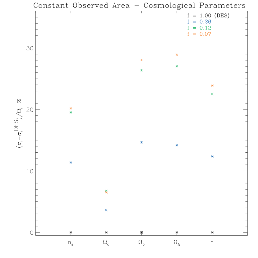
Figure 9 shows the relative gain in the marginalised errors of each of the cosmological parameters with respect to DES. The largest gain for a sparse observation of the sky is on $\Omega_{\Lambda}$ with $\delta\Omega_{\Lambda}/\Omega_{\Lambda}\sim 27\%$ and the smallest is for $\Omega_{c}$ with a gain of $\delta\Omega_{c}/\Omega_{c}\sim 7\%$. Again, a qualitatively different scenario is seen for the non-marginalised errors; $\Omega_{b}$ has the largest gain due to sparsity, and $h$ has the smallest.

Figure 7: ‘Constant observed area’ — Figure of Merit for galaxy power spectrum bins on the left and cosmological parameters on the right. In this case the Entropy, A-optimality and D-optimality all decrease with $f$. And the overall changes in all the FoM are much larger than the ones seen in the previous scenario. It seems that the increase in the total size of the survey due to sparsity can make up for the aliasing that the sparse design induces. Overall we gain a great deal by spending the same amount of time on larger but sparsely sampled area. Note that the $f=0.07$ case is only for illustration purposes as it covers an area larger than the area of the sky.

Figure 8: ‘Constant observed area’ — Top panel shows the diagonal elements of the Fisher matrix for different $f$ for the power spectrum bins. As we sparsify the survey these elements increase, hence better constrain the spectrum. The bottom panel shows the row of the Fisher matrix that corresponds to the middle bin of the spectrum. Going away from the peak, the elements show the correlation between the different bins and the middle one. For DES the middle bins has a correlation with the close neighbouring bins. But the correlation decreases as we go away from the peak. Towards small $k$, large scales, it starts to increase again due to the sample variance. As $f$ decreases and we get more and more sparse, the middle bin has a sharper drop (due to the larger total size of the survey) i.e., less correlation with neighbouring bins. However, there is more aliasing between distant bins. Also, there are peaks (i.e., larger correlations) at certain scales which are related to the distances between the patches, which changes case by case. The DES survey, as a full contiguous survey, has indeed the least aliasing, while the sparsest survey has the most aliasing. Note that the $f=0.07$ case is only for illustration purposes as it covers an area larger than the area of the sky.

Figure 9: ‘Constant observed area’ — Relative change in the errors of the cosmological parameters. The largest gain is about $27\%$ by sparsifying the survey. Note that the $f=0.07$ case is only for illustration purposes as it covers an area larger than the area of the sky.

6 Conclusion

In this work we have investigated the advantages and disadvantages of sparsely sampling the sky as opposed to a contiguous observation. By making use of Bayesian Experimental Design, we have defined our Figure of Merit as different functions of the Fisher matrix. These FoM capture different aspects of the parameters of interest such as their overall variance, the correlation between them or a measure of both as in Entropy. By optimising these functions we investigate an optimal survey design for estimating the galaxy power spectrum and a set of cosmological parameters. We have compared a series of sparse designs to a contiguous design of DES. We split the area of the DES survey into small square patches and sparsify the survey in two ways:

1. by shrinking the size of the patches while they are kept at a constant position. In this case the total sampled area of the survey is constant while the observed area (and the survey observing time) shrinks. This means the total information gained from the survey reduces in each case. In this scenario all the three FoM (A-optimality, D-optimality and Entropy) increase with $f$, both for the power spectrum bins and the cosmological parameters. This is expected as a contiguous sampling should capture all the information and constrain cosmology the best. However, we note that this increase with decreasing sparsity is very small for both the bins and the cosmological parameters. Looking at the variance and the covariance of the parameters, we note that the slight degrading of the surveys due to sparsity is mostly because of the increased correlation between the bins — aliasing — rather than the the increased errors. In general we conclude that total aliasing induced by sparsity is small and the loss in the constraining power of the survey because of it is negligible. Hence, overall, little is gained by observing the sky more contiguously. Indeed the largest loss in terms of the errors of the cosmological parameters is of the order of $\sim 4.5\%$ in the sparsest case.

2. by keeping the size of the patches constant, but placing them further and further from one another. In this scenario the observed area (and observing time) is kept constant, while sparsifying means larger and larger total sampled area. This means the total information gained from the survey in each case is the same. Therefore, there are the two competing factors; one is the increase in the total sampled area as the survey is sparsified and the other is aliasing induced due to the larger and larger sparse mask on the sky.

   In this case all FoM decrease with $f$, and the change in the FoM is much larger than the ones seen in the previous scenario. As we sparsify the survey the decrease in errors makes up for the increased aliasing induced and hence cause a general improvement in constraining power of the survey. Overall we gain a great deal by spending the same amount of time on larger but sparsely sampled area. Indeed we gain as much as $\sim 27\%$ on the sparsest survey, which is a significant improvement.

We conclude that sparse sampling could be a good substitute for the contiguous observations and indeed the way forward for future surveys. At least for small areas of the sky, such as that of DES, sparse sampling of the sky can have less cost and less observing time, while obtaining the same amount of constraints on the cosmological parameters. On the other hand we can spend the same amount of time but sparsely observe a larger area of the sky. This greatly improves the constraining power of the survey.

In this work we have chosen square observation patches, which may be the worst shape in terms of the correlation they induce. Yet another constraint in this design is the fixed and determined positions of the patches which cause a loss of information at certain scales. The advantage of this approach has been its analytical formalism, which has made it possible to understand the important factors in the sparse sampling. For future work we will investigate an optimal shape foe the patches and have a numerical approach where these patches are randomly distributed on the sky. This causes an even loss of information on all scales and is expected to improve results greatly.

References

- Adelman-McCarthy et al. (2008) Adelman-McCarthy J. K., et al., 2008, Astrophys. J. Suppl., 175, 297
- Blake et al. (2006) Blake C., Parkinson D., Bassett B., Glazebrook K., Kunz M., Nichol R. C., 2006, MNRAS, 365, 255
- Bond et al. (1998) Bond J. R., Jaffe A. H., Knox L., 1998, PRD, 57, 2117
- Croom et al. (2004) Croom S. M., et al., 2004, Mon. Not. Roy. Astron. Soc., 349, 1397
- Kaiser (1984) Kaiser N., 1984, APJL, 284, L9
- Kaiser (1986) Kaiser N., 1986, MNRAS, 219, 785
- Laureijs (2009) Laureijs R., 2009, ArXiv e-prints
- Liddle et al. (2006) Liddle A., Mukherjee P., Parkinson D., 2006, Astronomy and Geophysics, 47, 040000
- Parkinson et al. (2007) Parkinson D., Blake C., Kunz M., Bassett B. A., Nichol R. C., Glazebrook K., 2007, MNRAS, 377, 185
- Peebles (1973) Peebles P., 1973, APJ, 185, 413
- Tegmark (1997) Tegmark M., 1997, Physical Review Letters, 79, 3806
- The Dark Energy Survey Collaboration (2005) The Dark Energy Survey Collaboration 2005, ArXiv Astrophysics e-prints
- Trotta (2007a) Trotta R., 2007a, MNRAS, 378, 72
- Trotta (2007b) Trotta R., 2007b, MNRAS, 378, 819
- Trotta (2007c) Trotta R., 2007c, MNRAS, 378, 819