The Baade-Becker-Wesselink technique and the fundamental astrophysical parameters of Cepheids

Abstract

The BBW method remains one of most demanded tool to derive full set of Cepheid astrophysical parameters. Surface brightness version of the BBW technique was preferentially used during last decades to calculate Cepheid radii and to improve PLC relations. Its implementation requires a priory knowledge of Cepheid reddening value. We propose a new version of the Baade–Becker–Wesselink technique, which allows one to independently determine the colour excess and the intrinsic colour of a radially pulsating star, in addition to its radius, luminosity, and distance. It is considered to be a generalization of the Balona light curve modelling approach. The method also allows calibration of the function $F(CI_{0})=BC(CI_{0})+10\times log(T_{eff}(CI_{0}))$ for the class of pulsating stars considered. We apply this technique to a number of classical Cepheids with very accurate light and radial-velocity curves. The new technique can also be applied to other pulsating variables, e.g. RR Lyraes. We also discuss the possible dependence of the projection factor on the pulsation phase.

1 Introduction

Classical Cepheids are the key standard candles. They are used to set the zero point of the extragalactic distance scale [Freedman et al. (2001), (Freedman et al 2001)] and also serve as important tracers of young populations [Binney and Merrifield (1998), (Binney and Merrifield 1998)]. They owe their popularity to their high luminosities and photometric variability (which make them easy to identify and observe even at large distances) and the fact that the luminosities, intrinsic colours, and ages of these stars are closely related to such an easy-to-determine quantity as the period of variability.

It would be best to calibrate the Cepheid period-luminosity (PL), period-colour (PC), and period-luminosity-colour relations using distances based on trigonometric parallaxes. However, the most precisely measured parallaxes of even the nearest Cepeheids remain insufficiently accurate and, more importantly, they may be fraught with so far uncovered systematic errors. Here the Baade–Becker–Wesselink method [Baade (1926, Becker (1940), Wesselink (1946), (BBW; Baade 1926, Becker 1940, Wesselink 1946)] comes in handy, because it allows the Cepheid distances (along with the physical parameters of these stars) to be inferred, thereby providing an independent check of results based on geometric methods (e.g., trigonometric and statistical parallaxes). The surface brightness technique was used most frequently and effectively during the past few decades. It is based on the relation between so-called limb-darkened surface brightness parameter and the normal colours of Cepheids [Barnes and Evans (1976), (Barnes and Evans 1976)]. Moreover, it critically depends on the adopted reddening value.

Cepheid reddening values can be estimated from medium- and broad-band photometric observations (including multicolour PL relations) and from spectroscopic data [Dean, Warren and Cousins (1978), Fernie (1987), Fernie (1994), Fer94, Fernie et al. (1995), Berdnikov et al. (1996), Berdnikov et al. (2000), Andrievsky et al. (2002, Andrievsky et al. (2002, Kovtyukh et al. 2008, Kim et al. (2011), (Dean, Warren and Cousins 1978, Fernie 1987, Fernie 1990, 1994, Fernie et al. 1995, Berdnikov, Vozyakova and Dambis 1996, Berdnikov, Dambis and Vozyakova 2000, Andrievsky et al. 2002a, b, Kovtyukh et al. 2008, Kim, Moon and Yushchenko 2011)]. All these methods use proper calibrations and relationships between key stellar parameters. However, there exist large (up to $0.2mag$) scatter in the estimates of the colour excess for individual Cepheids, and the structure of the Cepheid instability strip is still vague. In the review on the Hubble constant and the Cepheid distance scale [Madore and Freedman (1991), Madore and Freedman (1991)] noted that “…any attempt to disentangle the effects of differential reddening and true color deviations within the instability strip must rely first on a precise and thoroughly independent determination of the intrinsic structure of the period-luminosity-color relation.” And next: “…independent reddenings and distances to individual calibrator Cepheids must be available.”

It should also be noted that reliable values of the colour excess and of the total-to-selective extinction ratio, say, $A_{V}/E(V-I)$, are extremely important when we use Wesenheit function to derive Cepheid luminosities from precise trigonometric parallaxes [Groenewegen an Oudmaijer (2000), Sandage et al.(2006), van Leewen 2007, (Groenewegen and Oudmaijer 2000, Sandage et al. 2006, van Leewen et al. 2007)]. To convert Wesenheit index $W_{VI}$ to the absolute magnitude, $M_{V}$, the intrinsic colour of the Cepheid, $(V-I)_{0}$, and the proper value of $A_{V}/E(V-I)$ are needed. We suppose that self-consistent and independent reddening estimates for individual Cepheids can reduce underestimated systematical errors induced by large variations of the absorption law [Fitzpatrick and Massa (2007), (Fitzpatrick and Massa 2007)] and can even result in $A_{\lambda}$ law in optics and NIR. Therefore, the search for independent estimates of Cepheid reddening values is still actual, and this is our primary aim.

Both BBW techniques – surface brightness (radius-variation modelling) and maximum likelihood (light-curve modelling) – are based on the same astrophysical background but make use somewhat different calibrations (limb-darkened surface brightness parameter, bolometric correction – effective temperature pair) on the normal colours. Here we propose a generalization of the [Balona (1977), Balona (1977)] light-curve modelling technique, which allows one to independently determine not only the star’s distance and physical parameters, but also the amount of interstellar reddening, and even calibrate the dependence of a linear combination of the bolometric correction and effective temperature on intrinsic colour [Rastorguev and Dambis (2011), (Rastorguev and Dambis 2011)].

2 Theoretical background

We now briefly outline the method. First, the bolometric luminosity of a star at any time instant is given by the following relation, which immediately follows from the Stefan–Boltzmann law:

$$L/L_{\odot}=(R/R_{\odot})^{2}\times(T/T_{\odot})^{4}.$$ (1)

Here $L$, $R$, and $T$ are the star’s current bolometric luminosity, radius, and effective temperature, respectively, and the $\odot$ subscript denotes the corresponding solar values. Given that the bolometric absolute magnitude, $M_{bol}$, is related to bolometric luminosity as

$$M_{bol}=M_{{bol}\odot}-2.5\times log(L/L_{\odot}),$$

we can simply derive from Eq. (2.1):

$$M_{bol}-M_{{bol}\odot}=-5\times log(R/R_{\odot})-10\times log(T/T_{\odot})$$ (2)

Now, $M_{bol}$ can be written in terms of the absolute magnitude $M$ in some photometric band and the corresponding bolometric correction, $BC$, i.e.

$$M_{bol}=M+BC,$$

and the absolute magnitude $M$ can be written as:

$$M=m-A-5\times log(d/10~{}pc).$$

Here $m$, $A$, and $d$ are the star’s apparent magnitude and interstellar extinction in the corresponding photometric band, respectively, and $d$ is the heliocentric distance of the star in pc. We can therefore rewrite Eq. (2.2) as follows:

$$m=A+5\times log(d/10~{}pc)+M_{{bol}\odot}+10\times log(T_{\odot})$$

$$-5\times log(R/R_{\odot})-BC-10\times log(T).$$ (3)

Let us introduce the function $F(CI_{0})=BC+10\times\log(T)$, the apparent distance modulus $(m-M)_{app}=A+5\times log(d/10~{}pc)$, and rewrite Eq. (2.3) as the light curve model:

$$m=Y-5\times log(R/R_{\odot})-F.$$ (4)

where constant

$$Y=(m-M)_{app}+M_{{bol}\odot}+10\times log(T_{\odot}).$$

We now recall that interstellar extinction, $A$, can be determined from the colour excess $CE$ as $A=R_{\lambda}\times CE$, where $R_{\lambda}$ is the total-to-selective extinction ratio for the passband-colour pair considered, whereas $M_{{bol}\odot}$, $R_{\odot}$, and $T_{\odot}$ are rather precisely known quantities. The quantity $F(CI_{0})=BC+10\times log(T)$ is a function of intrinsic colour index $CI_{0}=CI-CE$. [Balona (1977), Balona (1977)] used a very crude approximation for the effective temperature and bolometric correction, reducing the right-hand of the light curve model (2.4) to the linear function of the observed colour, with the coefficients containing the colour excess in a latent form.

The key point of our approach is that the values of function $F$ are computed from the already available calibrations of the bolometric correction $BC(CI_{0})$ and the effective temperature $logT(CI_{0})$  [Flower (1996), Bessell, Castelli and Plez (1998), Alonso et al. (1999), Sekiguchi and Fukugita (2000), Ramirez and Melendez (2005), Biazzo et al. (2007), Gonzalez Hernandez and Bonifacio (2009), (Flower 1996, Bessel, Castelli and Plez 1998, Alonso, Arribas and Martinez-Roger 1999, Sekiguchi and Fukugita 2000, Ramirez and Melendez 2005, Biazzo et al. 2007, Gonzalez Hernandez and Bonifacio 2009)]. These calibrations are expressed as high-order power series in the intrinsic colour:

$$F(CI_{0})=a_{0}+\sum^{N}_{k=1}a_{k}\cdot CI_{0}^{k},$$ (5)

with known $\{a_{k}\}$ and $N\leq 7$; in some cases the decomposition also includes the metallicity, $[Fe/H]$, and/or gravity ($log~{}g$) terms.

As for the stellar radius, $R$, its current value can be determined by integrating the star’s radial-velocity curve over time, using $dt=(P/2\pi)\cdot d\varphi$:

$$R(t)-R_{0}=-PF\cdot\int^{\varphi}_{\varphi_{0}}{(V_{r}(t)-V_{\gamma})\cdot(P/2\pi)\cdot d\varphi},$$

where $R_{0}$ is the radius value at the phase $\varphi_{0}$ [we use mean radius, $<R>=(R_{min}+R_{max})/2$ ]; $V_{\gamma}$ the systemic radial velocity; $\varphi$ the current phase of the radial velocity curve, $P$ the star’s pulsation period, and $PF$ the projection factor that accounts for the difference between the pulsation and radial velocities. Given the observables (light curve and apparent magnitudes, $m$, colour curve and apparent colour indices, $CI$, and radial velocity curve and $V_{r}$) and known quantities for the Sun, we end up with the following unknowns: distance, $d$, mean radius, $<R>$, and colour excess, $CE$, which can be found simply using a maximum-likelihood technique (nonlinear optimization).

For Cepheids with large amplitudes of light and colour curves ($\Delta CI\geq 0.4mag$), it is also possible to apply a more general technique by setting the expansion coefficients $\{a_{k}\}$ in Eq. (2.5) free and treating them as unknowns. We expanded the function $F=BC+10\times log(T)$ in Eq. (2.4) into a power series of the intrinsic colour index $CI_{0}^{st}$ of a well-studied “standard” star (e.g., $\alpha$ Per or some other bright star) with accurately known $T^{st}$:

$$F=BC^{st}+10\times log(T^{st})+\sum^{N}_{k=1}a_{k}\cdot(CI-CE-CI_{0}^{st})^{k}$$ (6)

The best fit to the light curve is provided with the optimal expansion order $N\simeq 5-9$. We use this modification to calculate the physical parameters and reddening $CE$ of the Cepheids, as well as the calibration $F(CI_{0})=BC(CI_{0})+10\times log(T_{eff}(CI_{0}))$ for a star of given metallicity $[Fe/H]$ and $log~{}g$ cite[(Rastorguev and Dambis 2011)]RD11.

3 Observational data, constants, and best calibrations

Cepheid photometric data were obtained by L. Berdnikov; his extensive multicolor photoelectric and CCD photometry of classical Cepheids is described in [Berdnikov (1995), Berdnikov (1995)]. Very accurate radial-velocity measurements of 165 northern Cepheids were measured with Moscow CORAVEL spectrometer [Tokovinin (1987), (Tokovinin 1987)] during the period 1987-2011 [Gorynya et al. (1992), Gorynya et al. (1996), Gorynya et al. (1998), (Gorynya et al. 1992, 1996, 1998)]. The total number of individual measurements is about 11,000 (the latest data are currently being prepared for publication). The photometric and spectral data sets are nearly synchronous, to prevent any systematic errors in the computed radii (up to 30$\%$) and other parameters owing to evolutionary period changes resulting in phase shifts between light, colour and radial velocity variations. We adopt $T_{\odot}$ = 5777 K, $M_{bol\odot}=+4.76^{m}$ [Gray (2005), (Gray 2005)]. We proceeded from $(V,B-V)$ data and found as the best solutions for the $V$-band light curve and $(B-V)$ color curve those computed using the $F[(B-V)_{0}]$ function based on two calibrations [Flower (1996), Bessell, Castelli and Plez (1998), (Flower 1996, Bessel, Castelli and Plez 1998)] of similar slope; the poorer results obtained using the other cited calibrations can be explained by the fact that the latter involved an insufficient number of supergiant stars.

4 The projection factor

There is yet no consensus as to which projection factor (PF) should be used for Cepheid variables  [Nardetto et al. (2004), Groenewegen (2007), Nardetto et al. (2007), Nardetto et al. (2009), (Nardetto et al. 2004, Groenewegen 2007, Nardetto et al. 2007, Nardetto et al. 2009)]. Different approaches (constant or period-dependent $PF$ values) lead to systematic differences in the inferred Cepheid parameters, first and foremost in the radii.

Bearing in mind the specific features of CORAVEL measurements,  [Rastorguev (2010), Rastorguev (2010)] introduced phase-dependent $PF$. Its value is calculated from flux integration across the stellar limb and depends on limb darkening coefficient, $\epsilon$ (linear darkening law $D(\varphi)=1-\epsilon+\epsilon\;cos\varphi,\;\varphi$ is the angle between line-of-sight direction and the surface element normal vector), and the photospheric velocity, $dr/dt$. The true line profile will be broadened by any spectral instrument, and usually we approximate it by Gaussian curve to measure the radial velocity as the coordinate of the maximum (see Fig. 1). In this case, the measured radial velocity will additionally depend on the instrument’s spectral linewidth, $S_{0}$ (so $PF$ value should be ”adjusted” to the spectrograph used for radial-velocity measurements), and on the photospheric velocity, $|dr/dt|$.

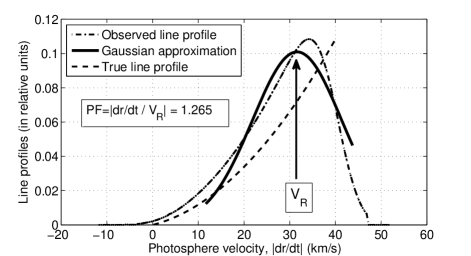
Figure 1: Example: true line profile ($\epsilon=0.75,dr/dt=40\;km/s$), observed line profile and its Gaussian approximation (with a spectrograph instrumental line width of $S_{0}=4\;km/s$). The measured $V_{R}$ value is indicated by the arrow; the $PF$ value is shown.

Figure 2: Projection factor, $PF$, as a function of $|dr/dt|$ for an instrumental width of $S_{0}=6\;km/s$ and for different values of limb-darkening coefficient $0.5<\epsilon<1$.

$PF$ values were estimated for $2.5<|dr/dt|<60\;km/s;\;0<\epsilon<1;\;4<S_{0}<8\;km/s$. We see, that the maximum of the normal approximation is shifted relative to the tip of the line profile. This shift depends on $|dr/dt|$ and $S_{0}$. Fig. 2 shows that the calculated $PF$ values may differ considerably from the “standard” and widely used value $PF=1.31$. Variations of $PF$ have also been reported by, e.g. Nardetto et al. (2004). We provide useful analytic approximation for the projection factor, $PF$, as a three-parameter exponential expression, based on 10,000 numerical experiments  [Rastorguev (2010), (Rastorguev 2010)]:

$PF\approx a_{1}\cdot exp[-(dr/dt)^{2}/(2\cdot a_{2}^{2})]+a_{3}$, where $a_{1},a_{2},a_{3}$ are functions of $\epsilon$ and $S_{0}$:

$a_{1}\approx-0.068\cdot\epsilon-0.0078\cdot S_{0}+0.217$

$a_{2}\approx+1.69\cdot\epsilon+2.477\cdot S_{0}+9.833$

$a_{3}\approx-0.121\cdot\epsilon+0.009\cdot S_{0}+1.297$

Overall, the $rms$ residual for this analytical expression is approximately 0.003. In practice, the $PF$ value for measured a given radial velocity should be determined by iteration for known values of $S_{0}$. To compare our results on Cepheids with other calculations, we finally adopted a moderate dependence of $PF$ on the period advocated by  [Nardetto et al. (2007), Nardetto et al. (2007)], although we repeated all calculations with other variants of $PF$ dependence on the period and pulsation phase to assure the stability of the calculated colour excess.

5 Results and discussion

To test the new method, we used the maximum-likelihood technique to solve Eq. (2.3) for the $V$-band light curve and $B-V$ colour curve for several classical Cepheids residing in young open clusters: SZ Tau, CF Cas, U Sgr, DL Cas, and GY Sge, and found good agreement for the calculated reddening values with those determined for the host clusters [Rastorguev and Dambis (2011), (Rastorguev and Dambis 2011)]. A weak sensitivity of calculated reddening, $E_{B-V}$, on the adopted $PF$ value (constant or period/phase-dependent) is explained by the very strong dependence of the light curve’s amplitude on effective temperature, $\sim 10\times log(T)$, and – as a consequence – on the dereddened colour. Although the internal errors of the reddening $E_{B-V}$ seem to be very small, the values determined using the two best calibrations  [Flower (1996), Bessell, Castelli and Plez (1998), (Flower 1996, Bessel, Castelli and Plez 1998)], may differ by as much as $0.03-0.05^{m}$, due to the systematic shift between these two calibrations. Fig. 3 shows the final fit to the $V$-band light curves for some Cepheids of our sample.

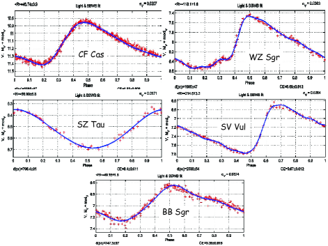
Figure 3: Examples of the light-curve modelling. Crosses: observations; solid line: model. Fit quality: $rms\sim 0.02-0.04mag$.

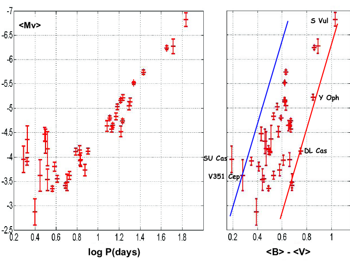
Figure 4: PL relation (left) and the instability strip (right) for approximately 40 Milky Way Cepheids. Intensity mean absolute magnitudes and colours are shown. Most of short-period Cepheids seem to be overtone pulsators. Cepheids residing near the edges of the instability strip and labeled by their names all have very small amplitudes of the light and colour curves.

PL relation and the instability strip for our Cepheid sample are shown on Fig. 4. Note that the inferred radii and luminosities of large fraction of the Cepheids with $P<4^{d}$ are too large for fundamental tone pulsations; in most cases this may be indirectly evidenced by their low colour amplitudes.

To refine the calibration $F(CI_{0})$ (2.6), we tried to use $\alpha$ Per as the “standard” star, with $T^{st}\approx(6240\pm 20)~{}K$, $[Fe/H]\approx-0.28\pm 0.06$ [Lee et al. (2006), (Lee et al. 2006)], $(B-V)^{st}\approx 0.48^{m}$ and $E_{B-V}\approx 0.09^{m}$ (WEBDA, for $\alpha$ Per cluster). To take into account the effect of metallicity on the zero-point $F(CI_{0})^{st}$, we estimated the gradient $dF(CI_{0})^{st}/d[Fe/H]\approx+0.24$ from the calibrations by [Alonso et al. (1999), Sekiguchi and Fukugita (2000), Gonzalez Hernandez and Bonifacio (2009), Alonso et al. 1999, Sekiguchi & Fukugita 2000, Gonzalez Hernandez & Bonifacio 2009]. In some cases (particularly for large-amplitude color variations) the “free” calibration, i.e. Eq. (2.6), can markedly improve the model fit to the observed light curve of the Cepheid variable. Fig. 5 shows the example of calibrations of the $F$ functions derived from nine Cepheids with different $[Fe/H]$ and $log~{}g$ values. The temperature scatter at $T_{eff}\sim 6600-5100~{}K$ amounts to $3-5\%$.

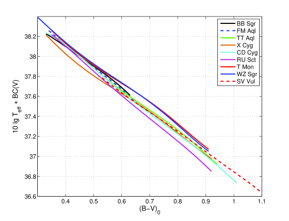
Figure 5: Inferred calibrations of the $F((B-V)_{0})$ function, Eq. (2.6), for nine Cepheids with large amplitudes of their colour variation.

When applied to an extensive sample of Cepheid variables with homogeneous photometric data and detailed radial-velocity curves, the new method is expected to lead to a completely independent scale of Cepheid reddening values and to refine the PL relation.

References

- [Alonso et al. (1999)] Alonso, A., Arribas, S., Martinez-Roger, C. 1999, AsApSuppl, 140, 261
- [Andrievsky et al. (2002] Andrievsky, S. M., Kovtyukh, V. V., Luck, R. E., et al. 2002 A&A, 381, 32
- [Andrievsky et al. (2002] Andrievsky, S. M., Kovtyukh, V. V., Luck, R. E., et al. 2002 A&A, 392, 491
- [Baade (1926] Baade, W. 1926, AN, 228, 359
- [Balona (1977)] Balona, L. A. 1976, MNRAS, 178, 231
- [Barnes and Evans (1976)] Barnes, T. G., Evans, D. S. 1976, MNRAS, 174, 489
- [Becker (1940)] Becker, W. 1940, ZA, 19, 289
- [Berdnikov (1995)] Berdnikov, L. N. 1995, In: Astrophysical applications of stellar pulsation. Proc. of IAU Colloq. No.155 held in Cape Town, South Africa, 6-10 February 1995; eds. Stobie, R. S. and Whitelock, P.A., Astronomical Society of the Pacific Conference Series, 83, 349.
- [Berdnikov et al. (1996)] Berdnikov, L. N., Vozyakova, O. V., Dambis, A. K. 1996, AstL, 22, 839
- [Berdnikov et al. (2000)] Berdnikov, L. N., Dambis, A. K., Vozyakova, O. V. 2000, A&AS, 143, 211
- [Bessell, Castelli and Plez (1998)] Bessell, M. S., Castelli, F., Plez, B. 1998, A&A, 333, 231
- [Biazzo et al. (2007)] Biazzo, K., Frasca, A., Catalano, S., et al. 2007, AN, 328, 938
- [Binney and Merrifield (1998)] Binney, J. and Merrifield, M. 1998, Galactic astronomy, Princeton, NJ : Princeton University Press
- [Dean, Warren and Cousins (1978)] Dean, J. F., Warren, P. R., Cousins, A. W. 1978, MNRAS, 183, 569
- [Fernie (1987)] Fernie, J. D. 1987, AJ, 94, 1003
- [Fernie (1990)] Fernie, J. D. 1990, ApJ, 354, 295
- [Fernie (1994)] Fernie, J. D. 1994, ApJ, 429, 844
- [Fernie et al. (1995)] Fernie, J. D., Evans, N. R., Beattie, B., Seager, S. 1995, IBVS, 4148, 1
- [Fitzpatrick and Massa (2007)] Fitzpatrick, E. L., Massa, D. 2007, ApJ, 663, 320
- [Flower (1996)] Flower, Ph. J. 1996, ApJ, 469, 355
- [Freedman et al. (2001)] Freedman, W. L., Madore, B. F., Gibson, B. K., et al. 2001, ApJ, 553, 47
- [Gonzalez Hernandez and Bonifacio (2009)] Gonzalez Hernandez, J. I., Bonifacio, P. 2009, A&A, 497, 497
- [Gorynya et al. (1992)] Gorynya, N. A., Irsmambetova, T. R., Rastorguev, A. S., Samus’, N. N. 1992, SvAtL, 18, 316
- [Gorynya et al. (1996)] Gorynya, N. A., Samus’, N. N., Rastorguev, A. S., Sachkov, M. E. 1996, AstL, 22, 175
- [Gorynya et al. (1998)] Gorynya, N. A., Samus’, N. N., Sachkov, M. E., Rastorguev, A. S., Glushkova, E. V., Antipin, S. 1998, AstL, 24, 815
- [Gray (2005)] Gray, C. D. F. 2005, The Observation and Analysis of Stellar Photospheres, Cambridge: Cambridge University Press
- [Groenewegen an Oudmaijer (2000)] Groenewegen, M., Oudmaijer, R. 2000, A&A 356, 849
- [Groenewegen (2007)] Groenewegen, M. A. T. 2007, A&A, 474, 975
- [Kim et al. (2011)] Kim, Chulee, Moon, B.-K., Yushchenko, A. V. 2011, JKAS, 43, 153
- [Kovtyukh et al. 2008] Kovtyukh, V. V., Soubiran, C., Luck, R. E., et al. 2008, MNRAS, 389, 1336
- [Lee et al. (2006)] Lee, B.-C., Galazutdinov, G. A., Han, I., et al. 2006, PASP, 118, 636
- [Madore and Freedman (1991)] Madore, B. F., Freedman, W. L. 1991, PASP, 103, 933
- [Nardetto et al. (2004)] Nardetto, N., Fokin, A., Mourard, D., et al. 2004, A&A, 428, 131
- [Nardetto et al. (2007)] Nardetto, N., Mourard, D., Mathias, Ph., et al. 2007, A&A, 471, 661
- [Nardetto et al. (2009)] Nardetto, N., Gieren, W., Kervella, P., et al. 2009, A&A, 502,951
- [Ramirez and Melendez (2005)] Ramirez, I., Melendez, J. 2005, ApJ, 626, 465
- [Rastorguev (2010)] Rastorguev, A. S. 2010, In: Variable Stars, the Galactic halo and Galaxy Formation, Proc. of an international conference held in Zvenigorod, Russia, 12-16 October 2009; eds. Sterken, Chr., Samus, N., Szabados, L., 225 (see also Rastorguev, A. S. “Variable stars, distance scale, globular clusters” arXiv:1001.1648v2)
- [Rastorguev and Dambis (2011)] Rastorguev, A. S., Dambis, A. K. 2011, AstrBull, 66, 47
- [Sandage et al.(2006)] Sandage, A., Tammann, G. A., Saha, A., et al. 2006, ApJ, 653, 843
- [Sekiguchi and Fukugita (2000)] Sekiguchi, M., Fukugita, M. 2000, AJ, 120, 1072
- [Tokovinin (1987)] Tokovinin, A. A. 1987, SvA, 31, 98
- [van Leewen 2007] van Leeuwen, F., Feast, M. W., Whitelock, P. A., et al. 2007, MNRAS, 379, 723
- [Wesselink (1946)] Wesselink, A.J. 1946, BAN, 10, 91