TUM-HEP-870/12
TTK-12-49
December 12, 2012

On “dynamical mass” generation in Euclidean de Sitter space

M. Beneke^a,b and P. Moch^a,b
aPhysik Department T31,
Technische Universität München,
James-Franck-Straße 1, D - 85748 Garching, Germany
^b Institut für Theoretische Teilchenphysik und Kosmologie,
RWTH Aachen University,
D–52056 Aachen, Germany

Abstract
We consider the perturbative treatment of the minimally coupled, massless, self-interacting scalar field in Euclidean de Sitter space. Generalizing work of Rajaraman, we obtain the dynamical mass $m^{2}\propto\sqrt{\lambda}H^{2}$ of the scalar for non-vanishing Lagrangian masses and the first perturbative quantum correction in the massless case. We develop the rules of a systematic perturbative expansion, which treats the zero-mode non-perturbatively, and goes in powers of $\sqrt{\lambda}$. The infrared divergences are self-regulated by the zero-mode dynamics. Thus, in Euclidean de Sitter space the interacting, massless scalar field is just as well-defined as the massive field. We then show that the dynamical mass can be recovered from the diagrammatic expansion of the self-energy and a consistent solution of the Schwinger-Dyson equation, but requires the summation of a divergent series of loop diagrams of arbitrarily high order. Finally, we note that the value of the long-wavelength mode two-point function in Euclidean de Sitter space agrees at leading order with the stochastic treatment in Lorentzian de Sitter space, in any number of dimensions.

1 Introduction

It is well-known that the free, massless, minimally coupled scalar field in the de Sitter background space-time cannot be defined in a de Sitter invariant way due to infrared (IR) divergences [1]. This occurs in any number of dimensions $d$, since the mode integral $\int d^{d-1}\vec{k}\,|\phi_{k}|^{2}$ that defines the Wightman two-point function always diverges logarithmically for $|\vec{k}\,|\to 0$. In the expanding cosmological coordinate frame the divergence arises from the red-shifting of modes, which leads to a pile-up of long-distance modes at late times. But non-interacting fields are not very interesting. The question arises whether upon turning on an interaction of the scalar quantum field, no matter how small, the IR problem could somehow cure itself. For this to happen, the interaction must effectively become non-perturbatively strong among the long-distance modes. If so, the non-perturbative dynamics may be too complicated to be solved with analytic methods. However, it may also be that after a suitable resummation or reorganization of the expansion in the interaction strength, the interacting, massless, minimally coupled scalar field lends itself to a well-defined, systematic treatment.

Various previous results suggest that in scalar field theory with a quartic self-interaction $-\lambda\phi^{4}/4!$ the originally massless field acquires a dynamical mass $m^{2}_{\rm dyn}\propto\sqrt{\lambda}H^{2}$, where $H$ is the Hubble constant of de Sitter space-time, which indeed regularizes the IR divergence. Starobinsky and Yokoyama [2] treat the long-distance fluctuations of the field as a classical random field that satisfies a Langevin equation. The associated Fokker-Planck equation is solved for large times by a probability distribution that results in finite correlation functions. Another approach uses the Schwinger-Dyson equations and obtains the dynamical mass from a self-consistent solution. In the mean-field or the large-$N$ limit [3, 4] the self-energy can be restricted to the one-loop, tadpole diagram. Garbrecht and Rigopoulos [5] analyzed the various in-in propagators in the CTP formalism and found that the large-$N$ result is modified by the two-loop self-energy, but remarkably, no further contribution arises beyond two loops due to systematic cancellations in the CTP index sums. However, while both formalisms agree on the parametric size $\sqrt{\lambda}H^{2}$ of the dynamical mass squared, the two exact results from [2, 5] disagree on the numerical prefactor. Neither of the formalisms so far explains how to compute sub-leading terms systematically.

The present work is motivated by the attempt to resolve the difference between the classical stochastic and diagrammatic/Schwinger-Dyson approach. For reasons that will become evident it is much simpler but still instructive to investigate the issue in Euclidean de Sitter space, which is simply the sphere $S^{d}$. In an elegant paper Rajaraman [6] considered the functional integral on the sphere and identified the zero-mode integral as the origin of non-perturbative dynamics. He computed the two-point function of the zero mode, which can be related to the dynamical mass. In this paper we extend the functional-integral approach and use 2PI methods to compute the exact self-energy, which is the central quantity in the diagrammatic approach. Our main results are as follows:

• We formulate the rules for a well-defined perturbation expansion of correlation functions of the massless, minimally coupled scalar field in Euclidean de Sitter space. The expansion parameter turns out to be $\sqrt{\lambda}$ instead of the coupling $\lambda$ of the standard perturbation expansion.

• For the massive scalar field we obtain the dependence of the dynamical mass on the Lagrangian mass $m$; for the massless field the leading ${\cal O}(\sqrt{\lambda})$ correction.

• We show that the dynamical mass can be obtained from the loop expansion of the self-energy after summing a divergent series to all orders in the loop expansion.

• It seems to have gone unnoticed that the Euclidean dynamical mass [6] agrees with the result from the stochastic approach. We show that this is true in an arbitrary number of space-time dimensions despite the fact that the relevant dimension-dependent quantities are apparently unrelated.

The interacting, massless, minimally coupled scalar field is therefore perfectly well-defined on the de Sitter background. For $\lambda\ll 1$ there is a systematic weak-coupling expansion. The reason why this is possible despite the fact that the zero mode is truly strongly coupled is that the infrared theory consists of a single degree of freedom (the zero mode), whose dynamics can be solved exactly. What all this implies for Lorentzian de Sitter space is less clear. We must leave this important point to further investigation.

2 Scalar field in Euclidean de Sitter space

Euclidean de Sitter space is obtained from $d$-dimensional de Sitter space in global coordinates with line element

$$ds^{2}=dt^{2}-\frac{1}{H^{2}}\,\cosh^{2}(Ht)\,d\Omega_{d-1}$$ (1)

by defining $t=-\frac{i}{H}\left(\theta-\frac{\pi}{2}\right)$ and assuming $2\pi i/H$ periodicity in $t$, which turns $ds^{2}$ into

$$ds^{2}=-g_{\mu\nu}dx^{\mu}dx^{\nu}=-\frac{1}{H^{2}}\left(d\theta^{2}+\sin^{2}\theta\,d\Omega_{d-1}\right).$$ (2)

Thus, Euclidean de Sitter space is equivalent to the $d$-dimensional sphere with radius $1/H$. Because the sphere is compact, functions admit a discrete mode expansion in spherical harmonics. In $d$ dimensions the spherical harmonics $Y_{\vec{L}\,}(x)$ are labelled by the integer index vector $\vec{L}=(L,L_{d-1},\ldots,L_{1})$ with $L\geq L_{d-1}\geq\ldots\geq L_{2}\geq|L_{1}|$ and satisfy (see, e.g., [7])

$$\Box\,Y_{\vec{L}}=\frac{1}{\sqrt{g}}\,\partial_{\nu}(\sqrt{g}g^{\nu\mu}\partial_{\mu}\,Y_{\vec{L}})=-H^{2}L(L+d-1)Y_{\vec{L}}$$ (3)

as well as the orthogonality relation

$$\int d^{d}x\sqrt{g(x)}\,Y^{*}_{\vec{L}}(x)Y_{{\vec{L}}^{\prime}}(x)=\frac{1}{H^{d}}\,\delta_{{\vec{L}}{\vec{L}}^{\prime}}.$$ (4)

The volume of Euclidean de Sitter space is

$$V_{d}=\int d^{d}x\sqrt{g(x)}=\frac{2\pi^{\frac{d+1}{2}}}{\Gamma(\frac{d+1}{2})H^{d}}=\frac{1}{Y_{0}^{2}H^{d}}.$$ (5)

Here $Y_{0}$ denotes the lowest harmonic, which is constant.

We consider the minimally coupled, real scalar field with Euclidean action

$$S = \int d^{d}x\sqrt{g}\left\{\frac{1}{2}\,g^{\mu\nu}\partial_{\mu}\phi\partial_{\nu}\phi+\frac{1}{2}m^{2}\phi^{2}+\frac{\lambda}{4!}\,\phi^{4}\right\}$$ (6)

$$= \frac{1}{2}\sum_{\vec{L}}\frac{1}{H^{d}}\,(H^{2}L(L+d-1)+m^{2})|\tilde{\phi}_{\vec{L}}|^{2}+S_{\rm int},$$

where the second line follows from the mode expansion

$$\phi(x)=\sum_{\vec{L}}\tilde{\phi}_{\vec{L}}\,Y_{\vec{L}}(x)$$ (7)

and the orthogonality relation (4). From the quadratic terms of (6) we deduce the free propagator

$$G_{\rm free}(x,x^{\prime}) = \sum_{\vec{L},\vec{L}^{\prime}}Y_{\vec{L}}(x)\,G_{\vec{L}\vec{L}^{\prime}}Y^{*}_{\vec{L}^{\prime}}(x^{\prime})=\sum_{\vec{L}}H^{d}\,\frac{Y_{\vec{L}}(x)Y^{*}_{\vec{L}}(x^{\prime})}{H^{2}L(L+d-1)+m^{2}}$$ (8)

$$= \frac{H^{d-2}}{(4\pi)^{d/2}}\,\frac{\Gamma(\frac{d-1}{2}+\nu)\Gamma(\frac{d-1}{2}-\nu)}{\Gamma(\frac{d}{2})}\,{}_{2}F_{1}\left(\frac{d-1}{2}+\nu,\frac{d-1}{2}-\nu;\frac{d}{2};1-\frac{y}{4}\right)\qquad$$

with

$$y=2\left(1-\cos\theta\cos\theta^{\prime}-\sin\theta\sin\theta^{\prime}\,\vec{w}\cdot\vec{w}^{\prime}\,\right)\quad\mbox{and}\quad\nu=\sqrt{\left(\frac{d-1}{2}\right)^{2}-\frac{m^{2}}{H^{2}}}\,.$$ (9)

Here $y$ is the invariant distance on the $d$-sphere $S^{d}$, and $\vec{w}$, $\vec{w}^{\prime}$ are two unit vectors on the sub-sphere $S^{d-1}$ with solid angle element $d\Omega_{d-1}$ in (2). The second line of (8) is indeed the de Sitter propagator in the Bunch-Davies vacuum [8, 9] in imaginary time.

The free propagator is ill-defined for $m=0$. The leading term for small $m$ is

$$G_{\rm free}(x,x^{\prime})\stackrel{{\scriptstyle m\to 0}}{{\rightarrow}}\frac{H^{d}}{(4\pi)^{d/2}}\,\frac{\Gamma(d)}{\Gamma(\frac{d}{2})}\times\frac{1}{m^{2}},$$ (10)

which, as can be seen from the first line of (8), originates only from the zero mode. Let us separate the constant zero mode from the field by defining

$$\phi(x)=\phi_{0}+\hat{\phi}(x).$$ (11)

The free propagator is the sum of the zero mode and non-zero mode propagator, since cross terms vanish by angular momentum conservation. The free zero-mode propagator equals the right-hand side of (10) for any $m=0$ /    , while the non-zero-mode propagator has a well-defined massless limit. In $d=4$,

$$\hat{G}_{\rm free}(x,x^{\prime})=\frac{H^{2}}{4\pi^{2}}\left(\frac{1}{y}-\frac{1}{2}\ln\frac{y}{4}-1\right)\qquad(m=0).$$ (12)

From now on we consider the massless, scalar field, $m=0$, unless mentioned otherwise, and assume $\lambda\ll 1$. The free zero-mode propagator is not defined, which is not surprising, since the zero mode has no quadratic term in the action (6). The zero-mode must be treated non-perturbatively. Let

$$G(x,x^{\prime})=G_{0}+\hat{G}(x,x^{\prime})=\langle\phi_{0}\phi_{0}\rangle+\langle\hat{\phi}(x)\hat{\phi}(x^{\prime})\rangle$$ (13)

be the exact two-point function of the interacting theory. Since $G_{0}$ is constant, we may write

$$G_{0}\equiv\frac{H^{d}Y_{0}^{2}}{m_{\rm dyn}^{2}}=\frac{\Gamma(\frac{d+1}{2})H^{d}}{2\pi^{\frac{d+1}{2}}m_{\rm dyn}^{2}}=\frac{1}{V_{d}m_{\rm dyn}^{2}}.$$ (14)

Comparison with the $L=0$ term in the first line of (8) suggests that we identify $m_{\rm dyn}^{2}$ with the dynamical mass of the originally massless scalar field, generated by the self-interaction. Note that this interpretation should be regarded with some caution, since the value of $m_{\rm dyn}^{2}$ is not related to the decrease of correlation functions at large separation $1/m_{\rm dyn}$. In fact, $1/m_{\rm dyn}$ corresponds to distances parametrically larger than the radius of the sphere, which carry no meaning. Similarly, in Lorentzian de Sitter space a dynamical mass of order $\lambda^{1/4}H\ll H$ is related to super-horizon correlations. Nevertheless, as will be seen below, a finite value of $G_{0}$ regularizes the IR divergence of the massless field and allows us to define a well-behaved perturbation expansion.

3 Perturbation expansion on the sphere

In [6] the zero-mode two-point function $\langle\phi_{0}\phi_{0}\rangle$ was computed by evaluating the dominant contribution to its functional-integral representation, which gives

$$m_{\rm dyn}^{2}=\frac{\Gamma(\frac{1}{4})}{\sqrt{4!}\,\Gamma(\frac{3}{4})}\,\sqrt{\frac{1}{H^{d}V_{d}}}\,\sqrt{\lambda}H^{d/2}.$$ (15)

In the following we generalize this approach. We show that both, $\langle\phi_{0}\phi_{0}\rangle$ and $\langle\hat{\phi}(x)\hat{\phi}(x^{\prime})\rangle$ have well-defined perturbation expansions in $\sqrt{\lambda}$, and provide a set of Feynman rules for this expansion.

The generating functional is conveniently written in terms of two separate sources $J_{0}$, $\hat{J}(x)$, for the zero- and non-zero-mode field, respectively:

$$Z[J_{0},\hat{J}] = N\int{\cal D}[\phi_{0}]{\cal D}[\hat{\phi}]\,\exp\left(-S-\int d^{d}x\sqrt{g}\,(J_{0}\phi_{0}+\hat{J}\hat{\phi})\right)$$ (16)

$$= \exp\left(-S_{\rm int}\!\left[\frac{\delta}{\delta J_{0}},\frac{\delta}{\delta\hat{J}}\right]\right)\,Z_{0}[J_{0}]\,\hat{Z}_{\rm free}[\hat{J}],$$

where $N$ is defined such that $Z[0,0]=1$. Here

$$S_{\rm int}[\phi_{0},\hat{\phi}]=\frac{\lambda}{4!}\int d^{d}x\sqrt{g}\left(\hat{\phi}^{4}+4\phi_{0}\hat{\phi}^{3}+6\phi_{0}^{2}\,\hat{\phi}^{2}\right),$$ (17)

and the term proportional to $\phi_{0}^{3}\hat{\phi}$ vanishes since $\int d^{d}x\sqrt{g}\,Y_{\vec{L}}(x)=0$ for $L>0$. The key point is that the term $\frac{\lambda}{4!}\,\phi_{0}^{4}$ is not included in $S_{\rm int}$, but must be part of $Z_{0}[J_{0}]$, since in the absence of a mass term for the scalar field the quadratic term in the zero-mode action vanishes, and the integral over $\phi_{0}$ in $Z_{0}[J_{0}]$ does not converge for large field values [6]. Hence,

$$Z_{0}[J_{0}]=N_{0}\int{\cal D}[\phi_{0}]\,\exp\left(-\int d^{d}x\sqrt{g}\left(\frac{\lambda}{4!}\,\phi_{0}^{4}+J_{0}\phi_{0}\right)\right),$$ (18)

while the generating functional for the free non-zero-mode field,

$$\hat{Z}_{\rm free}[\hat{J}] = \hat{N}\int{\cal D}[\hat{\phi}]\,\exp\left(-\int d^{d}x\sqrt{g}\,\left(\frac{1}{2}\,g^{\mu\nu}\partial_{\mu}\hat{\phi}\partial_{\nu}\hat{\phi}+\hat{J}\hat{\phi}\right)\right)$$ (19)

$$= \exp\left(\frac{1}{2}\int d^{d}x\sqrt{g}\int d^{d}y\sqrt{g}\,\hat{J}(x)\hat{G}_{\rm free}(x,y)\hat{J}(y)\right),$$

is a standard Gaussian functional integral. The zero-mode functional integral is simply an ordinary one-dimensional integral. Moreover, $\phi_{0}$ and $J_{0}$ are independent of $x$, so $\int d^{d}x\sqrt{g}=V_{d}$ in (18). The integral over $\phi_{0}$ can be evaluated exactly. Introducing

$$\tilde{\lambda}=\frac{\lambda}{4!}V_{d},\qquad\tilde{J}_{0}=J_{0}V_{d},$$ (20)

we find

$$Z_{0}[J_{0}] = N_{0}\int_{-\infty}^{\infty}d\phi_{0}\,\exp\left(-\tilde{\lambda}\,\phi_{0}^{4}-\tilde{J}_{0}\phi_{0}\right)$$ (21)

$$= {}_{0}F_{2}\!\left(\frac{1}{2},\frac{3}{4};\frac{\tilde{J}_{0}^{4}}{256\tilde{\lambda}}\right)+\frac{\Gamma\left(\frac{3}{4}\right)}{2\Gamma\left(\frac{1}{4}\right)}\frac{\tilde{J}_{0}^{2}}{\sqrt{\tilde{\lambda}}}\,\,{}_{0}F_{2}\!\left(\frac{5}{4},\frac{3}{2};\frac{\tilde{J}_{0}^{4}}{256\tilde{\lambda}}\right),$$

where ${}_{0}F_{2}$ denotes a hypergeometric function. One easily checks that

$$\langle\phi_{0}^{2}\rangle_{0}=\frac{\delta^{2}}{\delta\tilde{J}_{0}^{2}}\,Z_{0}[J_{0}]_{|J_{0}=0}=\frac{1}{\sqrt{\tilde{\lambda}}}\,\frac{\Gamma\left(\frac{3}{4}\right)}{\Gamma\left(\frac{1}{4}\right)}$$ (22)

reproduces (15) as is should be. Similarly, $\langle\phi_{0}^{2n}\rangle_{0}$ follows from taking the appropriate number of derivatives. The index 0 on the bracket means that the computation is done with the zero-mode functional $Z_{0}$ alone. The full zero-mode $n$-point functions computed from $Z$ in (16) receive sub-leading corrections, as discussed below.

It is now straightforward to develop a systematic perturbative expansion of (16) and the corresponding Feynman rules. From (18) it follows that every zero-mode fields counts as $\lambda^{-1/4}$, while $\hat{\phi}$ has the standard counting 1. The interaction $\frac{\lambda}{4}\phi_{0}^{2}\hat{\phi}^{2}$ therefore counts as $\sqrt{\lambda}$. In general, since there is always an even number of $\phi_{0}$ involved, correlation functions have an expansion in $\sqrt{\lambda}$. The rules are as follows: For a given correlation function expand (16) to the desired order in $\lambda$ using the above counting rules. Perform the standard Wick contractions of pairs of non-zero mode fields. This can be represented in terms of lines and vertices in the usual way. However, no Wick contractions are to be performed for the zero-mode fields. Instead, collect all factors of $\phi_{0}$ and compute the expectation value of $\langle\phi_{0}^{2n}\rangle_{0}$ exactly.

As an example, we evaluate the first correction to the zero-mode and non-zero-mode two-point functions. For the zero-mode case, we have

$$\langle\phi_{0}\phi_{0}\rangle = \langle\phi_{0}^{2}\rangle_{0}+\langle\phi_{0}^{4}\rangle_{0}\,\times\,\ \includegraphics{a.eps}\,$$ (23)

$$= \langle\phi_{0}^{2}\rangle_{0}-\frac{\lambda}{4}\,\langle\phi_{0}^{4}\rangle_{0}\int d^{d}x\sqrt{g}\,\hat{G}_{{\rm free}}^{{\rm ren}}(x,x)+{\cal O}(\sqrt{\lambda}),$$

where the black square represents the $\frac{\lambda}{4}\phi_{0}^{2}\hat{\phi}^{2}$ vertex. If we define $\langle\phi_{0}\phi_{0}\rangle\equiv 1/(V_{d}m_{\rm dyn}^{2})$ as before in (14) and denote the previously obtained leading-order expression (15) by $m_{\rm dyn,0}^{2}$, the previous equation translates into

$$m_{\rm dyn}^{2}=m_{\rm dyn,0}^{2}\left(1+\sqrt{\lambda}\,\frac{3\,\Gamma(\frac{1}{4})}{2\sqrt{4!}\,\Gamma(\frac{3}{4})}\,\sqrt{V_{d}}\,\hat{G}_{\rm free}^{\rm ren}(x,x)+{\cal O}(\lambda)\right),$$ (24)

where $\langle\phi_{0}^{4}\rangle_{0}=1/(4\hat{\lambda})$ has been used. While the leading expression $m_{\rm dyn,0}^{2}$ is unambiguous, the first correction depends on the UV subtraction that defines the coincident non-zero-mode propagator $\hat{G}_{\rm free}^{\rm ren}(x,x)$. To be specific, consider the case of four dimensions. In dimensional regularization one needs to take $x^{\prime}\to x$ before expanding the $d=4-2\epsilon$ dimensional propagator $\hat{G}_{\rm free}(x,x^{\prime})$ around $d=4$, in which case

$$\hat{G}_{\rm free}^{\rm reg}(x,x)=\frac{H^{2}}{(4\pi)^{2}}\left[\frac{2}{\hat{\epsilon}}+2\ln\frac{\mu^{2}}{H^{2}}-7+4\gamma_{E}\right].$$ (25)

The $\overline{\rm MS}$-renormalized value corresponds to this expression with the pole term in $\frac{1}{\hat{\epsilon}}=\frac{1}{\epsilon}-\gamma_{E}+\ln(4\pi)$ in brackets subtracted. Further, $\mu$ is the $\overline{\rm MS}$ renormalization scale. We note that the dynamical mass is not by itself a physical quantity. While the leading term is unambiguous, the first correction involving the propagation of non-zero modes is scheme- and scale-dependent.

The non-zero-mode two-point function is the free propagator in leading order. Including the ${\cal O}(\sqrt{\lambda})$ correction it reads

$$\langle\hat{\phi}(x)\hat{\phi}(x^{\prime})\rangle = \hat{G}_{\rm free}(x,x^{\prime})+\langle\phi_{0}^{2}\rangle_{0}\,\times\,\parbox{241.84842pt}{ {\centering\includegraphics{b.eps}\@add@centering}}$$ (26)

$$= \hat{G}_{\rm free}(x,x^{\prime})-\frac{\lambda}{2}\,\langle\phi_{0}^{2}\rangle_{0}\int d^{d}z\sqrt{g}\,\hat{G}_{\rm free}(x,z)\hat{G}_{\rm free}(z,x^{\prime})+{\cal O}(\lambda)$$

$$= \sum_{\vec{L}=\hskip-3.32504pt/\;0}H^{d}\,\frac{Y_{\vec{L}}(x)Y^{*}_{\vec{L}}(x^{\prime})}{H^{2}L(L+d-1)}\left(1-\frac{\lambda\langle\phi_{0}^{2}\rangle_{0}}{2H^{2}L(L+d-1)}+{\cal O}(\lambda)\right).$$

The expression for the leading correction differs from [6]. The diagram computed there is part of the sub-leading ${\cal O}(\lambda)$ correction. In four dimensions the leading term equals (12), and the leading $\sqrt{\lambda}$ correction can also be summed to give

$$-\frac{\lambda\langle\phi_{0}^{2}\rangle_{0}}{48\pi^{2}}\left[\mbox{Li}_{2}(u)+\left(\frac{1}{2u}-2\right)\ln(1-u)-\frac{\pi^{2}}{6}+\frac{1}{9}\right],$$ (27)

where $u=1-y/4$.

4 Schwinger-Dyson equation

We now return to the approaches pursued in [3, 5, 4] which are based on evaluations of the scalar-field self-energy and the Schwinger-Dyson equation

$$\Box_{x}G(x,x^{\prime})=\frac{1}{\sqrt{g(x)}}\,\delta^{(d)}(x-x^{\prime})+\int d^{d}w\,\sqrt{g(w)}\,\Pi(x,w)G(w,x^{\prime}).$$ (28)

We project this equation on the zero-mode component by integrating over $x^{\prime}$ and using the identity

$$\int d^{d}x\,\sqrt{g(x)}\,Y_{\vec{L}}(x)=\frac{\delta_{\vec{L}0}}{H^{d}Y_{0}},$$ (29)

which follows from (4). This results in

$$0=1+V_{d}^{2}\Pi_{0}G_{0}.$$ (30)

In the spirit of the 2PI formalism (see below) we regard the self-energy as a functional of the exact propagator and derive it from the functional derivative

$$\Pi(x,x^{\prime})=2\,\frac{\delta\Gamma_{\rm 2PI}^{\rm rest}}{\delta G(x,x^{\prime})}$$ (31)

of the 2PI effective action with the classical and one-loop term subtracted (as denoted by “rest”) [10]. The loop expansion of the effective action is given by

$$\Gamma_{\rm 2PI}^{\rm rest} = \parbox{51.21495pt}{ {\centering\includegraphics{c1.eps}\@add@centering}}\,+\,\parbox{31.29802pt}{ {\centering\includegraphics{c2.eps}\@add@centering} }\,+\,\parbox{31.29802pt}{ {\centering\includegraphics{c3.eps}\@add@centering}}\,\,+\,\parbox{31.29802pt}{ {\centering\includegraphics{c4.eps}\@add@centering} }\,\,+\,\parbox{31.29802pt}{ {\centering\includegraphics{c5.eps}\@add@centering} }\,\,+\,{\cal O}(\lambda^{5})$$ (32)

$$\frac{1}{8} \frac{1}{48} \frac{1}{48} \frac{1}{128} \frac{1}{32}$$

$$= \sum_{n=1}^{\infty}\alpha_{n}(-\lambda)^{n}\int d^{d}x_{1}\sqrt{g(x_{1})}\ldots\int d^{d}x_{n}\sqrt{g(x_{n})}\,\underbrace{G(.,.)\ldots G(.,.)}_{2n\,\,\rm factors}\,,$$

where $\alpha_{n}$ denotes the combinatorial factor associated with a diagram, as given in the first line, and where we have given the explicit diagrammatic representation up to the five-loop order. Instead of appealing to the 2PI formalism we could have written down the self-energy diagrams directly with the proviso that all internal lines are exact rather than free propagators.

The power-counting rules of the previous section tell us that the leading contribution to $\Gamma_{\rm 2PI}^{\rm rest}$ and $\Pi_{0}$ is obtained from pure zero-mode diagrams, that is, every full propagator is replaced by $G_{0}$. Since every loop brings one factor of $\lambda$ from the new vertex and adds two propagators, which each count as $1/\sqrt{\lambda}$, we conclude that every order in the loop expansion contributes to the leading term. This shows that the loop expansion must be summed to all orders to obtain the correct value of the “dynamical mass” in Euclidean de Sitter space.

To see this explicitly, note that upon plugging the derivative of (32) into (30), the latter equation can be solved for $G_{0}$, which yields the value of $m_{\rm dyn}^{2}$. (More precisely, $m_{\rm dyn,0}^{2}$ since by replacing $G$ by $G_{0}$ in (32) we pick up the leading term only.) The functional derivative in (31) eliminates two integrations in (32) such that an $n$-loop self-energy diagram contributes $\alpha_{n}(-\lambda)^{n}V_{d}^{n-2}G_{0}^{2n-1}$ to (30). Therefore, with the ansatz $G_{0}=(\lambda V_{d})^{-1/2}\times z$, where $z$ is a number to be determined, and the explicit expression (32) for the loop expansion up to the four-loop self-energy, the Schwinger-Dyson equation (30) turns into

$$0=1-\frac{z^{2}}{2}+\frac{z^{4}}{6}-\frac{z^{6}}{4}+\frac{5z^{8}}{8}+\ldots\equiv f(z),$$ (33)

where the term $z^{2n}$ corresponds to the sum of $n$-loop self-energy diagrams. In terms of $z$, the “dynamical mass” is given by

$$m_{\rm dyn,0}^{2}=\frac{1}{z}\times\frac{\sqrt{\lambda}}{\sqrt{V_{d}}}\,\stackrel{{\scriptstyle d=4}}{{=}}\,\frac{1}{z}\times\frac{\sqrt{6\lambda}H^{2}}{4\pi}.$$ (34)

Keeping only the one-loop tadpole diagram in (33), which corresponds to truncation after the quadratic term, we obtain $z=\sqrt{2}$ and $m_{\rm dyn}^{2}=\sqrt{3\lambda}H^{2}/(4\pi)$ (in $d=4$), which coincides with the mean-field result [2] and the one-loop result in Lorentzian de Sitter space [3, 5, 4]. In the two-loop approximation, the quadratic equation for $z^{2}$ does not yield a real solution for $z$. Thus, at two loops there is a difference between the solution of the Schwinger-Dyson equation in Euclidean de Sitter space and the solution to the corresponding equations for the closed-time-path propagators in Lorentzian de Sitter space [5]. Continuing to higher orders in (33), at three loops, we find $z=1.166\ldots$, while at four loops (which includes the last term shown explicitly in (33)) there is again no solution. Thus, the loop expansion does not seem to converge to the exact value (15), which corresponds to

$$z=\sqrt{4!}\,\frac{\Gamma\left(\frac{3}{4}\right)}{\Gamma\left(\frac{1}{4}\right)}=1.65580\ldots.$$ (35)

The question arises how the exact result that is obtained easily from the functional integral is recovered diagrammatically. Clearly, we need the expansion of $f(z)$ to all orders. But this cannot be obtained from (32). While the integrations are trivial in the zero-mode approximation, the diagram topologies and computation of combinatorial factors become too complicated.

5 Zero-mode dynamics in the 2PI formalism

In the following we exploit the 2PI formalism [10, 11] to derive an expression that generates the perturbative expansion of the zero-mode self-energy to any desired order. We focus on the zero-mode dynamics which alone is responsible for the leading contributions as discussed above, and hence set $\hat{\phi}$ to zero. In this section we drop the subscript “0”, since all quantities are understood to refer to the zero mode.

The generating “functional” in the 2PI formalism is

$$Z[J,R] = e^{-W[J,R]}=N\int{\cal D}[\phi]\,\exp\left(-S[\phi]-\int_{x}J(x)\phi(x)-\frac{1}{2}\int_{x,y}R(x,y)\phi(x)\phi(y)\right)$$ (36)

$$= N\int_{-\infty}^{\infty}d\phi\,\exp\left(-\tilde{\lambda}\phi^{4}-\tilde{J}\phi-\frac{1}{2}\tilde{R}\phi^{2}\right),$$

where $\tilde{\lambda}$ and $\tilde{J}$ (equal to $\tilde{J}_{0}$) have been defined in (20), $\int_{x}\,[...]=\int d^{d}x\sqrt{g(x)}\,[...]$, and

$$\tilde{R}=V_{d}^{2}R.$$ (37)

The simple one-dimensional integral in the second line of (36) applies since the zero-mode field is constant. The exact propagator in the presence of the external sources can be found from the relation

$$\frac{dW}{d\tilde{R}}=\frac{1}{2}\left(\phi_{\rm cl}^{2}+G\right),$$ (38)

where $\phi_{\rm cl}=dW/d\tilde{J}$ is the field expectation value. Since the functional integral is an ordinary one-dimensional integral, the functional derivatives are actually ordinary derivatives. It follows from (21) that the field expectation value vanishes in the absence of the source $J$, that is, the symmetry $\phi\to-\phi$ is not spontaneously broken. This remains true for $J=0$ and $R=\!\!\!\!\!\!/\;0$. Since eventually we are interested in the theory in the absence of external sources we now put $J=0$ and consequently $\phi_{\rm cl}=0$. In this case we find the closed expression

$$Z[0,R]=e^{-W[0,R]}=\frac{\sqrt{\tilde{R}}}{4\sqrt{2}\,\Gamma(\frac{5}{4})\,\tilde{\lambda}^{1/4}}\,\exp\!\left(\frac{\tilde{R}^{2}}{32\tilde{\lambda}}\right)\,K_{\frac{1}{4}}\!\left(\frac{\tilde{R}^{2}}{32\tilde{\lambda}}\right),$$ (39)

where $K_{\nu}(x)$ denotes the modified Bessel function of the second kind. From (38) we obtain

$$G(R)=\frac{\tilde{R}}{8\tilde{\lambda}}\,\left(\frac{K_{\frac{3}{4}}\!\left(\frac{\tilde{R}^{2}}{32\tilde{\lambda}}\right)}{K_{\frac{1}{4}}\!\left(\frac{\tilde{R}^{2}}{32\tilde{\lambda}}\right)}-1\right)=\frac{H^{d}Y_{0}^{2}}{m^{2}_{\rm dyn}(R)}.$$ (40)

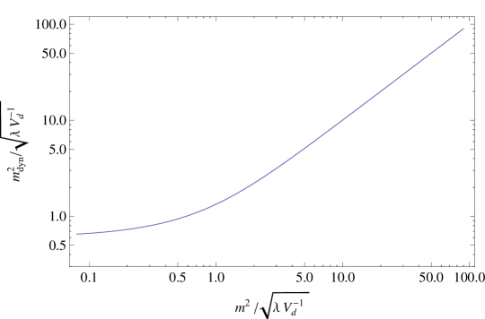
Figure 1: Dynamical mass of the zero mode as function of the Lagrangian mass.

The previous equation gives the exact zero-mode propagator or, equivalently, the “dynamical mass” of the zero mode in the presence of the propagator source $R$. We note that since $R$ is constant, $V_{d}R$ has an equivalent interpretation as a Lagrangian mass $m^{2}$ for the scalar field. Hence (40) provides the “dynamical mass” of the scalar field for arbitrary $m$, generalizing the expression (15) for the massless case [6]. The dependence of $m^{2}_{\rm dyn}$ on $m^{2}$ is sketched in Figure 1. At large $m^{2}$ the “dynamical mass” asymptotes to $m^{2}$ with ordinary perturbative corrections of order $\lambda$, as should be expected, since the infrared enhancement that renders the zero-mode dynamics non-perturbative is cut off for a sufficiently massive scalar field. For $m^{2}\to 0$, the “dynamical mass” tends to the value (15). The pre-asymptotic corrections can be determined easily by expanding (40) around the corresponding limits.

6 Diagrammatic zero-mode self-energy to all orders

We now determine the self-energy that is needed to solve the Schwinger-Dyson equation. In the 2PI formalism, the Schwinger-Dyson equation reads

$$G^{-1}(R)=G^{-1}_{\rm free}+\tilde{R}-\Pi(G).$$ (41)

The inverse free propagator is $G^{-1}_{\rm free}=-12\tilde{\lambda}\phi_{\rm cl}^{2}$, which vanishes for $J=0$. This reflects once more the fact that the free propagator of the massless scalar field is ill-defined in the absence of external sources. Thus,

$$\Pi(G)=-\frac{1}{G}+\tilde{R}(G).$$ (42)

It follows that the diagrammatic expansion of the self-energy is obtained by inverting $G(R)$ given in (40), and expanding it in powers of $\lambda$.

While a closed expression for the inverse of $G(R)$ may not exist, we can solve for the expansion in $\lambda$ by making the ansatz

$$\tilde{R}(G)=\frac{1}{G}+a_{1}\lambda V_{d}G+a_{2}{\lambda}^{2}V_{d}^{2}G^{3}+\ldots,$$ (43)

where the first term is required by (42) to obtain a regular perturbative expansion of $\Pi(G)$. The term $a_{n}\lambda^{n}V_{d}^{n}G^{2n+1}$ represents the sum of the $n$-loop diagrams to the zero-mode self-energy, expressed in terms of the exact zero-mode propagator. The definition of the expansion coefficients $a_{n}$ is chosen such that with the definition (34) of $z$ the function $f(z)$ defined in (33) is given by

$$f(z)=1-\sum_{n=1}^{\infty}a_{n}z^{2n}.$$ (44)

Plugging the ansatz (43) into (40) and matching coefficients in the expansion in $\tilde{\lambda}$ (equivalently, in $G$), we find the $a_{n}$. The first ten terms are shown in Table 1. We note that the first four agree with (33) obtained from the combinatorial factors of the lowest-order Feynman-diagram topologies. We determined the exact coefficients up to $n=200$, which turn out to be rational numbers of increasing length.

$n$	1	2	3	4	5	6	7	8	9	10
$a_{n}$	$-\frac{1}{2}$	$\frac{1}{6}$	$-\frac{1}{4}$	$\frac{5}{8}$	$-\frac{101}{48}\vphantom{\frac{\sum_{i=0}^{\infty}}{\sum_{i=0}^{\infty}}}$	$\frac{279}{32}$	$-\frac{8143}{192}$	$\frac{271217}{1152}$	$-\frac{374755}{256}$	$\frac{51151939}{512}$

Table 1: The first ten series coefficients $a_{n}$.

Inspection of the $a_{n}$ coefficients shows that they form a sign-alternating, factorially divergent series with

$$a_{n}\;\stackrel{{\scriptstyle n\to\infty}}{{\sim}}\;0.201...\times\left(-\frac{2}{3}\right)^{n}\,n!\times\left(1-\frac{1.7...}{n}+\ldots\right).$$ (45)

The divergent behaviour arises because the expansion in small $G$ corresponds to an expansion of $G(R)$ around $R=\infty$, see (43), while the value of $m^{2}_{\rm dyn}$ is related to $G(R)$ at $R=0$. The divergent series is also the reason why we did not obtain a reasonable approximation to $m^{2}_{\rm dyn}$ from the low-order approximations to the self-energy.

It remains to show that the Schwinger-Dyson approach is consistent with the exact result (15) for the “dynamical mass”, which requires summing the divergent series. To this end we construct the Borel transform of $f(z)$

$$B[f](u)=1-\sum_{n=1}^{\infty}a_{n}\,\frac{u^{n}}{n!},$$ (46)

such that the Borel sum $F(z)$ of $f(z)$ is given by

$$F(z)=\frac{1}{z^{2}}\int_{0}^{\infty}du\,e^{-u/z^{2}}\,B[f](u).$$ (47)

Since the series is sign-alternating, we expect $B[f](u)$ to exhibit a singularity on the negative axis, but without a closed expression we do not know the precise singularity structure of the Borel transform of $f$. Given (40), it is reasonable to assume that it is analytic in a vicinity of the positive real axis such that the Borel integral is well-defined, and to assume that the Borel sum $F(z)$ equals the original function $f(z)$.

Term-by-term integration of the series expansion of $B[f](u)$ simply returns the divergent series expansion of $f$. We therefore resort to a standard trick [12] and construct a Padé approximation from the truncated series expansion. More precisely, we use the first $2n$ coefficients of the expansion of $B[f]$, not counting the “1” in (46), and construct the diagonal $(n,n)$ Padé approximant. We use this approximation to $B[f](u)$ in the Borel integral (47) and obtain $F(z)$ by numerical integration. We then solve the equation $F(z_{*})=0$, see (33), to determine the “dynamical mass”. Alternatively, we can determine the solution of $f(z_{*})=0$ from Padé approximants to the expansion (44) of $f(z)$ directly, without going through the Borel transform. The results are shown in Table 2. The solutions are seen to quickly approach the exact result (35), especially when the Padé approximation is applied to the Borel transform, in which case one-permille accuracy is reached already for $n=3$. This demonstrates that the diagrammatic approach via the 2PI Schwinger-Dyson equation reproduces the path-integral result, as it must be, but only after summation of a divergent series expansion to all orders.

$n$	3	6	9	12	24	48	96
$z_{*}$ from $F$	1.65709	1.65635	1.65581	1.65580	1.65580	1.65580	1.65580
$z_{*}$ from $f$	1.71012	1.66262	1.65723	1.65618	1.65581	1.65580	1.65580

Table 2: Solution of $F(z_{*})=0$ (second line) and $f(z_{*})=0$ (third line) employing a diagonal $(n,n)$ Padé approximation constructed from the first $2n$ series coefficients $a_{k}$. The exact value is $z_{*}=\sqrt{4!}\,\Gamma\left(\frac{3}{4}\right)/\Gamma\left(\frac{1}{4}\right)=1.65580\ldots.$

7 Stochastic approach in $d$ dimensions

The methods applied above do not extend to Lorentzian de Sitter space, which is non-compact, and does not allow to identify the (leading) infrared dynamics with the one of a single zero-mode degree of freedom. However, quite some time ago Starobinsky and Yokoyama [2] suggested that the long-wavelength part of the scalar field can be treated as a classical stochastic variable, which satisfies a Langevin equation with a random force provided by the short-wavelength modes. Here we show that this leads to the same value for the two-point function of the long-wavelength field as the zero-mode two-point function in Euclidean de Sitter space, in any number of dimensions $d$. This intriguing coincidence seems not to have been noted before.

Following [2] we divide the scalar field into $\phi=\phi_{0}+\hat{\phi}$, where $\phi_{0}$ contains all long-wavelength modes with wave number $k<\epsilon aH$ with $a$ the scale factor and $\epsilon\ll 1$ the parameter that separates long from short wave-lengths. From the field equation it follows that $\phi_{0}$ satisfies the Langevin equation

$$\dot{\phi}_{0}(t,\vec{x})=-\frac{1}{(d-1)H}\,V^{\prime}(\phi_{0})+f(t,\vec{x}).$$ (48)

Here $V(\phi)$ is the scalar field potential and $f$ the stochastic force

$$f=\dot{\hat{\phi}}=\epsilon aH^{2}\int\frac{d^{d-1}k}{(2\pi)^{d-1}}\,\delta(k-\epsilon aH)\,\left(a_{k}\phi_{k}(t)e^{i\vec{k}\cdot\vec{x}}+\mbox{c.c.}\right)$$ (49)

generated by the short-distance modes. At leading order, we can neglect the self-interaction of the short-distance modes. The fluctuations satisfy $\langle f(t_{1},\vec{x})f(t_{2},\vec{x})\rangle=\alpha\delta(t_{1}-t_{2})$ with

$$\alpha=\frac{2\pi^{\frac{d-1}{2}}}{(2\pi)^{d-1}\Gamma(\frac{d-1}{2})}\times\frac{2^{d-3}\,[\Gamma(\frac{d-1}{2})]^{2}}{\pi}\times H^{d-1}$$ (50)

The first factor arises from the volume of the $d-2$ dimensional momentum shell $k=\epsilon aH$, the second from the long-wavelength limit (since $k=\epsilon aH\ll aH$) of the Bunch-Davies mode functions $\phi_{k}(t)$. The Fokker-Planck equation for the one-particle probability density $P[\varphi]$ associated with (48) is

$$\frac{\partial P}{\partial t}=\frac{1}{(d-1)H}\,\frac{\partial}{\partial\varphi}\,(V^{\prime}(\varphi)P)+\frac{\alpha}{2}\,\frac{\partial^{2}}{\partial\varphi^{2}}\,P,$$ (51)

which admits the stationary late-time solution

$$P[\varphi]=N\exp\left(-\frac{2}{(d-1)\alpha H}\,V(\varphi)\right),$$ (52)

in terms of which the two-point function of the (constant) long-wavelength field is given by

$$\langle\phi_{0}\phi_{0}\rangle=N\int_{-\infty}^{\infty}d\varphi\,\varphi^{2}\exp\left(-\frac{2}{(d-1)\alpha H}\,V(\varphi)\right).$$ (53)

This precisely agrees with (22) (for $V(\phi)=\frac{\lambda}{4!}\phi^{4}$) provided the dissipation and fluctuation coefficients in the Fokker-Planck equation are related to the volume of $d$-dimensional Euclidean de Sitter space with radius $1/H$ by

$$(d-1)H\times\frac{\alpha}{2}=\frac{1}{V_{d}},$$ (54)

which can be easily verified. Hence, the long-wavelength two-point functions (and therefore “dynamical masses”) are the same, as claimed. One may wonder why the result could be derived from zero-mode dynamics alone in Euclidean de Sitter space, while the fluctuations originated from the short-wavelength modes in the stochastic approach. However, the result from the latter is independent of $\epsilon$ in the above approximation, as it should be, and the stochastic force is generated by wave numbers $k=\epsilon aH$. We can take $\epsilon$ arbitrarily small and conclude that in the leading approximation the main contribution to the stochastic force can be assumed to originate from the boundary between long- and short wavelengths, which can be taken to be deep in the infrared.

We note that the stochastic approach can be derived rigorously from the full quantum dynamics in the leading logarithmic approximation in $a$ [13], which is equivalent to keeping the leading infrared-enhanced terms in Euclidean de Sitter space. But unlike the Euclidean case discussed in the present paper, a systematic method for calculating corrections around the Lorentzian result of [2] is not known.

8 Conclusion

In this paper we considered the perturbative treatment of the minimally coupled, massless, self-interacting scalar field in Euclidean de Sitter space. Generalizing the work of Rajaraman [6], we obtained the dynamical mass $m^{2}\propto\sqrt{\lambda}H^{2}$ of the scalar for non-vanishing Lagrangian masses, as well as the first perturbative quantum correction in the massless case, and developed the rules of a systematic perturbative expansion, which after treating the zero-mode non-perturbatively, goes in powers of $\sqrt{\lambda}$. We then showed how the dynamical mass can be recovered from the summation of the diagrammatic expansion of the self-energy and a consistent solution of the Schwinger-Dyson equation. This clarifies the relation between the path-integral and diagrammatic treatment, and implies that solutions based on truncations of the loop expansion can at best be approximate. With the proper exact treatment of the zero mode, the reorganized perturbative expansion is free from infrared divergences, which are present for the free, minimally coupled scalar field in Euclidean de Sitter space. The interacting, massless field is therefore well-defined, and the rules for generating the systematic perturbative expansion are almost as simple as the standard rules for the massive case.

What this implies for Lorentzian de Sitter space is much less clear. We showed that the long-wavelength mode two-point function computed in the stochastic approach of [2] coincides with the exact Euclidean result in leading order in the expansion in $\sqrt{\lambda}$. This strongly suggests to us that the dynamical mass of the self-interacting scalar field in de Sitter space can be obtained by some sort of analytic continuation from the Euclidean, up to higher-order corrections. It would be very interesting to derive this result diagrammatically, in the spirit of [5], and to understand how to develop a systematic expansion in Lorentzian de Sitter space.

Acknowledgement

We thank B. Garbrecht, T. Prokopec and G. Rigopoulos for discussions. This work is supported in part by the Gottfried Wilhelm Leibniz programme of the Deutsche Forschungsgemeinschaft (DFG).

References

- [1] B. Allen, Phys. Rev. D 32 (1985) 3136.
- [2] A. A. Starobinsky and J. Yokoyama, Phys. Rev. D 50 (1994) 6357, [astro-ph/9407016].
- [3] A. Riotto and M. S. Sloth, JCAP 0804 (2008) 030, arXiv:0801.1845 [hep-ph].
- [4] J. Serreau, Phys. Rev. Lett. 107 (2011) 191103, arXiv:1105.4539 [hep-th].
- [5] B. Garbrecht and G. Rigopoulos, Phys. Rev. D 84 (2011) 063516, arXiv:1105.0418 [hep-th].
- [6] A. Rajaraman, Phys. Rev. D 82 (2010) 123522, arXiv:1008.1271 [hep-th].
- [7] A. Higuchi, J. Math. Phys. 28 (1987) 1553 [Erratum-ibid. 43 (2002) 6385].
- [8] P. Candelas and D. J. Raine, Phys. Rev. D 12 (1975) 965.
- [9] D. Marolf and I. A. Morrison, Phys. Rev. D 82 (2010) 105032 [arXiv:1006.0035 [gr-qc]].
- [10] J. Berges, AIP Conf. Proc. 739 (2005) 3 [hep-ph/0409233].
- [11] J. M. Cornwall, R. Jackiw and E. Tomboulis, Phys. Rev. D 10 (1974) 2428.
- [12] J. Zinn-Justin, Quantum field theory and critical phenomena, Int. Ser. Monogr. Phys. 113 (2002) 1.
- [13] T. Prokopec, N. C. Tsamis and R. P. Woodard, Annals Phys. 323 (2008) 1324, arXiv:0707.0847 [gr-qc].