Two-nucleon scattering: merging chiral effective field theory with dispersion relations

Abstract

We consider two-nucleon scattering close to threshold. Partial-wave amplitudes are obtained by an analytic extrapolation of subthreshold reaction amplitudes calculated in a relativistic formulation of chiral perturbation theory. The constraints set by unitarity are used in order to stabilize the extrapolation. Neutron-proton phase shifts are analyzed up to laboratory energies $T_{{\rm lab}}\simeq 250$ MeV based on the next-to-next-to-next-to-leading order expression for the subthreshold amplitudes. We find a reasonably accurate description of the empirical S- and P-waves and a good convergence of our approach. These results support the assumption that the subthreshold nucleon-nucleon scattering amplitude may be computed perturbatively by means of the chiral expansion. The intricate soft scales that govern the low-energy nucleon-nucleon scattering are generated dynamically via a controlled analytic continuation.

1 Introduction

The last decade has witnessed an impressive progress towards a quantitative solution of the nuclear many-body problem starting from the underlying forces between the nucleons. Rapidly increasing available computational resources coupled with modern ab-initio few- and many-body methods as well as renormalization techniques to reduce the many-body model space make it nowadays possible, to carry out reliable and accurate nuclear structure calculations for light and even medium-mass nuclei. One can therefore directly relate the fine properties of the nuclear Hamiltonian to the spectra and other properties of nuclei without invoking any uncontrollable approximations. It is thus of utmost importance for contemporary nuclear physics and nuclear astrophysics, to develop a detailed, quantitative understanding of low-energy interactions between the nucleons based on QCD, the underlying theory of the strong force. Remarkable progress along these lines has been achieved in the past two decades within the framework of (chiral) effective field theory. In particular, accurate nucleon-nucleon (NN) potentials at next-to-next-to-next-to-leading order in the chiral expansion have been constructed Weinberg:1991um ; Ordonez:1992xp ; Entem:2003ft ; Epelbaum:2004fk . The corresponding developments for the three-nucleon force are underway, see Refs. Epelbaum:2008ga ; Machleidt:2011zz and references therein.

As a complementary approach, NN scattering can also be addressed from the standpoint of the dispersion relations. This method has been formulated and extensively explored in the sixties of the last century starting from the pioneering work by Goldberger et al. Goldberger:1960md , see also Refs. Ball:1965sa ; Scotti:1963zz ; Scotti:1965zz . Clearly, these studies were lacking a systematic theoretical framework to treat low-energy pion dynamics which is nowadays available in terms of chiral perturbation theory (ChPT). We also mention recent work Refs. Albaladejo:2011bu ; Albaladejo:2012sa along these lines, where the impact of the left-hand cut emerging from one-pion exchange on NN scattering is investigated. For recent applications of dispersion relations in combination with chiral perturbation theory to pion- and photon-nucleon dynamics the reader is referred to Refs. Gasparyan:2010xz ; Gasparyan:2010fb ; Gasparyan:2011yw ; Ditsche:2012fv .

In the present paper, we use these ideas as developed in the recent works Gasparyan:2010xz ; Gasparyan:2010fb ; Gasparyan:2011yw ; Danilkin:2011fz ; Danilkin:2012ua , which we call dispersive effective field theory (DEFT), to propose a novel approach to NN dynamics. It relies on the knowledge of the analytic structure of the NN $S$-matrix and makes use of the chiral expansion for the scattering amplitude, which is assumed to be valid in some region below threshold, coupled with the conformal mapping techniques to perform reliable extrapolations to higher energies.

The dispersive approach formulated and applied in this paper is complementary to methods based on potentials derived within ChPT which have been extensively explored in the past decade. We expect it to bring new insights into various aspects related to low-energy nucleon-nucleon scattering. First, given considerable progress in the derivation of nuclear forces in the framework of ChPT in recent years, it is important to unabiguously identify effects of the long-range chiral two-pion exchange potential in nucleon-nucleon scattering data, see e.g. Refs. Rentmeester:1999vw ; Birse:2003nz ; Rentmeester:2003mf ; Birse:2007sx ; Shukla:2008sp ; Birse:2010jr for some studies along these lines based on the potential framework. The dispersive approach relies on an explicit evaluation of the discontinuity across the low-lying left-hand cuts in the amplitude and thus provides a transparent and efficient way to identify long-range physics. Secondly, there is an ongoing discussion in the community on how to carry out nonperturbative renormalization of the Schrödinger equation in the framework of chiral effective field theory and possible implications for power counting, see Kaplan:1996xu ; Lepage:1997cs ; Beane:2001bc ; Nogga:2005hy ; Birse:2005um ; PavonValderrama:2005wv ; Epelbaum:2006pt ; Long:2011xw for samples of different views. Our dispersive approach is based on the on-shell scattering amplitude which, in the subthreshold region, is constructed using chiral perturbation theory without performing any nonperturbative resummations. Nonperturbative effects in the physical region are generated by solving the integral equation dictated by elastic unitarity. Our approach, therefore, allows to address the above-mentioned issues from a completely different perspective and might shed new light on this important problem. Last but not least, we also plan to apply this method in the future to investigate the possibility to treat the two-pion exchange potentials in perturbation theory which is considered as an option to formulate renormalizable approaches to NN scattering in chiral EFT.

Our manuscript is organized as follows. In section 2, we briefly describe the theoretical method we are using to compute the NN scattering amplitude. The chiral expansion for the discontinuities across the left-hand cuts is discussed in section 3. The results for NN phase-shifts are presented in section 4. Finally, our conclusions are summarized in section 5.

2 An analytic continuation of the NN scattering amplitude

A NN partial-wave amplitude has a well-known singularity structure as a function of the complex variable $s$. On the physical sheet, apart from the pole corresponding to the deuteron bound state in the ${}^{3}S_{1}-^{3}D_{1}$ channel, there are right- and left-hand cuts as shown in Fig. 1. The right-hand cuts correspond to intermediate states in the $s$-channel and start from the two-nucleon threshold, $s=4m_{N}^{2}$.

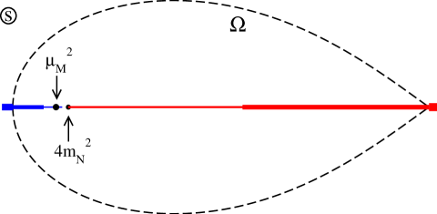
Figure 1: Cuts of the partial wave NN amplitude in the complex $s$-plane. The first, second and third left-hand cuts start at $s=4m_{N}^{2}-(nM_{\pi})^{2}$, $n=1,2,3$. The first and second right-hand cuts due to inelastic channels start at the one- and two-pion production thresholds $s=(2m_{N}+nM_{\pi})^{2}$ with $n=1,2$. Further, $\mu_{M}$ denotes the matching point as explained in the text.

The discontinuity of the amplitude across this cut is determined by the unitarity condition

$$\Delta T(s) \equiv \frac{1}{2\,i}\left(T(s+i\epsilon)-T(s-i\epsilon)\right)$$ (1)

$$= T(s+i\epsilon)\,\rho(s)\,T(s-i\epsilon)+\dots\,,$$

where the dots stand for inelastic channel contributions which start at the pion production threshold, $s=(2m_{N}+M_{\pi})^{2}$. The phase-space function $\rho(s)$ and the amplitude $T(s)$ in Eq. (1) turn into $2\times 2$ matrices for the coupled partial waves.

It is advantageous to discriminate between the two sources of branch cuts in the scattering amplitudes. The so-called generalized potential $U(s)$ collects all contributions emerging from the left-hand cuts only. Given the generalized potential, the full scattering amplitudes may be reconstructed in terms of the non-linear integral equation

$$T(s\,)=U(s\,)+\,\int_{4m_{N}^{2}}^{\infty}\frac{ds^{\prime}}{\pi}\,\frac{s-\mu_{M}^{2}}{s^{\prime}-\mu_{M}^{2}}\,\frac{T(s^{\prime})\,\rho(s^{\prime})\,T^{*}(s^{\prime})}{s^{\prime}-s-i\epsilon}\,.$$ (2)

Obviously, the solution of this equation recovers the right-hand cut in agreement with the elastic unitarity constraints. We further emphasize that the employed dispersion relations are sometimes written in the literature using non-relativistic variables, which is of course equivalent to the expressions used here. Since we neglect the contributions from inelastic channels in Eq. (1), $U(s)$ is well-defined only up to some $s=\Lambda_{s}^{2}$ below which the inelastic contributions are small. We choose this value to correspond to the two-pion production threshold $\Lambda_{s}=2m_{N}+2M_{\pi}$. The dependence of our results on a particular choice of $\Lambda_{s}$ will turn out to be rather weak, see section 4. At the matching point $s=\mu_{M}^{2}$, the scattering amplitude $T(s)$ per construction equals the generalized potential $U(s)$. We choose the matching point to be in the middle of the region between the unitarity $s$-channel cut and two-pion $t$-channel cut, i.e. $\mu_{M}^{2}=4m_{N}^{2}-2M_{\pi}^{2}$. The proper choice of the matching point is essential for the effectiveness of our approach. Our central assumption is a perturbative nature of the scattering amplitude near the matching point. Consequently, the generalized potential can be calculated at the matching point in the framework of ChPT. Upon performing an analytic continuation in the $s$-variable by employing a suitable chosen conformal mapping technique, the generalized potential $U(s)$ can be used in Eq. (2).

Consider the left-hand singularity structure of the generalized potential. The physically relevant cuts correspond to the $t$-channel one-pion and several-pion exchanges as visualized in Fig. 1. These cuts start at $s=4m_{N}^{2}-(nM_{\pi})^{2}$, where $n$ is the number of exchanged pions. We follow here the strategy of Gasparyan:2010xz and split the generalized potential into two parts,

$$U(s)=U_{\rm inside}(s)+U_{\rm outside}(s),$$ (3)

where $U_{\rm inside}(s)$ is calculated explicitly whereas $U_{\rm outside}(s)$ is analytically continued. In Fig. 1 we introduce a domain $\Omega$, which defines the separation of the ’inside’ and ’outside’ contributions to the generalized potential. The left and right-most point of the domain $\Omega$ are specified by $\Lambda^{2}$ (defined below) and $\Lambda_{s}^{2}$. The discontinuity across the left-hand cut from $s=4m_{N}^{2}-M_{\pi}^{2}$ to $s=4m_{N}^{2}-4M_{\pi}^{2}$ is unambiguously determined by the one-pion exchange contribution in terms of the $\pi NN$ coupling constant. It lies inside the domain $\Omega$ as shown in Fig. 1. The next part of the cut from $s=4m_{N}^{2}-4M_{\pi}^{2}$ to $s=4m_{N}^{2}-9M_{\pi}^{2}$ receives, in addition, the contributions from the two-pion exchange processes. We assume that in this energy region such contributions can be computed in ChPT and, therefore, they are also considered as part of $U_{\rm inside}(s)$. For $s<4m_{N}^{2}-9M_{\pi}^{2}$, the two-pion-exchange cut can no longer be reliably computed in perturbation theory. This reflects the nature of the $\pi\pi$ interaction in this kinematical region with its prominent and non-perturbative scalar-isoscalar channel. Therefore, we do not include this part into $U_{\rm inside}(s)$ and identify

$$U_{{\rm inside}}(s) = \int_{\Lambda^{2}}^{4m_{N}^{2}-M_{\pi}^{2}}\frac{ds^{\prime}}{\pi}\frac{\Delta T(s^{\prime})}{s^{\prime}-s}\,,$$

$$\Lambda^{2} = 4m_{N}^{2}-9M_{\pi}^{2}\,,$$ (4)

where $\Delta T(s)$ is the discontinuity of the amplitude across the cut. By definition, the ’outside’ part of the potential, $U_{\rm outside}(s)$, has singularities only outside the region $\Omega$ of Fig. 1. It incorporates, in particular, effects of three pion exchanges that are technically more challenging to compute. Since $U_{\rm outside}(s)$ is analytic inside $\Omega$, one may approximate it by a Taylor expansion around the NN threshold. The expansion coefficients would resemble the infinite tower of counter terms appearing in the chiral Lagrangian. However, such a series would converge only inside a circle with the radius $R=9M_{\pi}^{2}$ and, therefore, the generalized potential will be not suitable for using as input in Eq. (2) in order to compute the partial-wave scattering amplitudes in a controlled manner. We recall that the generalized potential is needed at least up to $s\approx 4m_{N}^{2}+8m_{N}M_{\pi}$ which is roughly $6$ times farther away from the NN threshold than accessible by that Taylor expansion with convergence radius $R=9M_{\pi}^{2}$.

Following Gasparyan:2010xz ; Danilkin:2010xd ; Danilkin:2011fz , we approximate $U_{\rm outside}(s)$ in the domain $\Omega$ of Fig. 1 in a systematic way by means of an appropriate conformal transformation. A function $\xi(s)$ having inverse $\zeta(\xi)$ that maps $\Omega$ onto a unit circle with $\xi(4m_{N}^{2})=0$ is constructed. The particular form of the conformal mapping is irrelevant. The potential $U_{\rm outside}(s)$ can now be expanded in a Taylor series in the conformal variable,

$$U_{{\rm outside}}(s\,) = \sum\limits_{k=0}^{n}{U_{k}}\,\big{[}\xi(s\,)\big{]}^{k}\,,$$

$$U_{k} = \frac{d^{k}U_{{\rm outside}}(\zeta(\xi))}{k!\,d\xi^{k}}\Big{|}_{\xi=0}\,,$$ (5)

that can be proven to converge in the full domain $\Omega$ of Fig. 1. The coefficients $U_{k}$ are determined by derivatives of $U_{{\rm outside}}$ at the expansion point $s=4m_{N}^{2}$. If the expansion in (5) is truncated at order $n$, the first $n$-derivatives need to be computed. We choose the number of terms $n+1$ in Eq. (5) to be equal to the number of local counter terms contributing to the considered partial wave in ChPT at a given order so that there is a one-to-one correspondence between Eq. (5) and the chiral expansion.

To be specific, we use here the conformal mapping suggested in Gasparyan:2010xz

$$\xi(s) = \frac{a_{1}\left(\Lambda^{2}_{s}-s\,\right)^{2}-1}{(a_{1}-2\,a_{2})\left(\Lambda^{2}_{s}-s\,\right)^{2}+1}\,,\;\;$$

$$a_{1} = \frac{1}{\left(\Lambda^{2}_{s}-4m_{N}^{2}\right)^{2}}\,,\;\;a_{2}=\frac{1}{\left(\Lambda^{2}_{s}-\Lambda^{2}\right)^{2}}\,.$$ (6)

A useful property of the transformation (6) is that it permits a smooth extrapolation of the generalized potential to a constant above $s=\Lambda^{2}_{s}$. Replacing in (5) the conformal map $\xi(s)$ by $\xi_{>}(s)$ defined as

$$\xi_{>}(s\,)=\left\{\begin{array}[]{ll}\xi(s\,)&{\rm for}\qquad s<\Lambda^{2}_{s}\,,\\ \xi(\Lambda^{2}_{s})&{\rm for}\qquad s\geq\Lambda^{2}_{s}\,,\end{array}\right.\quad\xi^{\prime}(\Lambda^{2}_{s})=0\,,$$ (7)

the outside potential is smoothly extended to a constant at energies $s>\Lambda_{s}^{2}$.

The final step in obtaining the amplitude in the physical region is to solve the integral equation (2) with respect to $T(s)$ for a given $U(s)$. A standard way of doing that is the so-called $N/D$ technique Chew:1960iv . The amplitude is represented as

$$T(s)=D^{-1}(s)N(s)\,,$$ (8)

where $D(s)$ has no singularities but the right-hand $s$-channel unitarity cuts. In contrast, the branch points of $N(s\,)$ correspond to those of $U(s\,)$. The unitarity condition implies

$$D(s\,)=1-\int_{4m_{N}^{2}}^{\infty}\frac{ds^{\prime}}{\pi}\,\frac{s-\mu_{M}^{2}}{s^{\prime}-\mu_{M}^{2}}\frac{N(s^{\prime})\,\rho(s^{\prime})}{s^{\prime}-s}\,.$$ (9)

The non-linear equation (2) reduces to the linear one for $N(s)$,

$$N(s\,) = U(s\,)+\int_{4m_{N}^{2}}^{\infty}\frac{ds^{\prime}}{\pi}\,\frac{s-\mu_{M}^{2}}{s^{\prime}-\mu_{M}^{2}}\,$$ (10)

$$\times \frac{N(s^{\prime})\,\rho(s^{\prime})\,[U(s^{\prime})-U(s\,)]}{s^{\prime}-s}\,,$$

which can be solved using standard numerical techniques.

It should be emphasized that apart from the dynamical singularities in the complex $s$-plane discussed above, the partial-wave amplitudes may have kinematic singularities or obey kinematic constraints. In particular, the standard $JLS$ amplitudes possess $\sqrt{s}$-type singularities and obey constraints at threshold, i.e. at $\sqrt{s}=\pm 2m_{N}$. Although, apart from constraints at $\sqrt{s}=2m_{N}$, they are located rather far away from the physical region, it is preferable to remove all of them if possible. A general method to achieve this goal for a system of two interacting spin-$1/2$ particles is presented in Stoica:2011cy and some particular cases were discussed in Ball:1965sa . We choose a set of amplitudes (which is generally speaking not unique) for the NN system as follows. For the uncoupled partial waves with $J=L$ and the ${}^{3}P_{0}$ channel, the $S$-matrix elements $S^{JLS}(s)$ or, equivalently, the phase shifts $\delta^{JLS}(s)$ are related with the amplitude $T^{JLS}(s)$ which is free of the kinematical singularities via

$$S^{JLS}(s)=e^{2\,i\,\delta^{JLS}(s)}=1+2\,i\,\rho_{L}(s)\,T^{JLS}(s)\,,$$ (11)

where the phase-space function is defined according to

$$\rho^{L}(s)=\frac{1}{8\pi}\left(\frac{1}{4}-\frac{m_{N}^{2}}{s}\right)^{L+\frac{1}{2}}\,.$$ (12)

For coupled partial waves, one needs, in addition, to perform a linear transformation of the $L=J\pm 1$ basis leading to the following relation in terms of the Stapp parametrization Stapp:1956mz

$$S^{J} = \left(\begin{matrix}\cos{2\epsilon_{J}}e^{2i\delta^{J-1}}&i\sin{2\epsilon_{J}}e^{i(\delta^{J-1}+\delta^{J+1})}\\ i\sin{2\epsilon_{J}}e^{i(\delta^{J-1}+\delta^{J+1})}&\cos{2\epsilon_{J}}e^{2i\delta^{J+1}}\end{matrix}\right)$$ (13)

$$= 1+2\,i\,\frac{1}{8\pi}\left(\frac{1}{4}-\frac{m_{N}^{2}}{s}\right)^{J-\frac{1}{2}}\,U^{T}\,T^{J}\,U\,,$$

with the transformation matrix

$$U=\left(\begin{matrix}\frac{2(J+1)m_{N}}{J\sqrt{s}}+1&\sqrt{\frac{J+1}{J}}\left(1-\frac{2m_{N}}{\sqrt{s}}\right)\\ \sqrt{\frac{J+1}{J}}\left(\frac{1}{4}-\frac{m_{N}^{2}}{s}\right)&\frac{m_{N}^{2}}{s}-\frac{1}{4}\,,\end{matrix}\right)\,,$$ (14)

which implies that the NN phase-space distribution has the form

$$\rho^{J} = \frac{2\,J+1}{8\pi J}\left(\frac{1}{4}-\frac{m_{N}^{2}}{s}\right)^{J-\frac{1}{2}}$$

$$\times \left(\begin{matrix}1+\frac{4m_{N}^{2}}{s}\frac{J+1}{J}&2\,\sqrt{\frac{J+1}{J}}\left(\frac{1}{4}-\frac{m_{N}^{2}}{s}\right)\frac{m_{N}}{\sqrt{s}}\\ 2\,\sqrt{\frac{J+1}{J}}\left(\frac{1}{4}-\frac{m_{N}^{2}}{s}\right)\frac{m_{N}}{\sqrt{s}}&\left(\frac{1}{4}-\frac{m_{N}^{2}}{s}\right)^{2}\end{matrix}\right).$$

3 Chiral perturbation theory for the left-hand cuts

We now discuss the derivation of the generalized potential in ChPT up to order $Q^{3}$ with $Q\sim M_{\pi}$ referring to a generic soft scale. The following terms in the effective Lagrangian are relevant for our calculation:

$$\mathcal{L}_{int} = -\frac{1}{4\,F_{\pi}^{2}}\,\bar{N}\,\gamma^{\mu}\,\big{(}\vec{\tau}\cdot\big{(}\vec{\pi}\times(\partial_{\mu}\vec{\pi})\big{)}\big{)}\,N$$ (15)

$$+ \frac{g_{A}}{2\,F_{\pi}}\,\bar{N}\,\gamma_{5}\,\gamma^{\mu}\,\big{(}\vec{\tau}\cdot(\partial_{\mu}\vec{\pi})\big{)}\,N$$

$$- \frac{2\,c_{1}}{F_{\pi}^{2}}\,M_{\pi}^{2}\,\bar{N}\,(\vec{\pi}\cdot\vec{\pi})\,N+\frac{c_{3}}{F_{\pi}^{2}}\,\bar{N}\,(\partial_{\mu}\,\vec{\pi})\cdot(\partial^{\mu}\vec{\pi})\,N$$

$$- \frac{c_{4}}{2\,F_{\pi}^{2}}\,\bar{N}\,\sigma^{\mu\nu}\,\big{(}\vec{\tau}\cdot\big{(}(\partial_{\mu}\vec{\pi})\times(\partial_{\nu}\vec{\pi})\big{)}\big{)}\,N\,.$$

Here, $\vec{\pi}$ and $N$ refer to pion and nucleon fields, $\vec{\tau}$ denote the isospin Pauli matrices while $F_{\pi}$ and $g_{A}$ are the pion decay and the nucleon axial vector constants, respectively. Further, $c_{i}$ are the low-energy constants (LECs) accompanying the subleading pion-nucleon vertices. For more details on the effective pion-nucleon Lagrangian the reader is referred to Refs. Fettes:1998ud ; Fettes:2000gb .

We apply the effective Lagrangian introduced above to compute the NN scattering amplitude to order $Q^{3}$. As already pointed out before, our central assumption is perturbativeness of the scattering amplitude in the region $s\sim\mu_{M}^{2}$ (see Ref. Danilkin:2010xd for a quantum-mechanical example). We, therefore, use here the standard chiral power counting based entirely on the naive dimensional analysis. Although we employ the manifestly Lorentz-invariant form of $\mathcal{L}_{int}$ without performing the $1/m_{N}$-expansion in order not to distort the discontinuity structure across the left-hand cuts, we apply the standard power counting rules of the heavy-baryon formulation and keep only those diagrams which do not vanish in the heavy-baryon framework at a given order. The Feynman diagrams emerging at various orders in the chiral expansion are depicted in Fig. 2.

$$T^{(0)} = \parbox{51.21504pt}{\includegraphics[width=51.21504pt,clip={true}]{one-pion_exchange.eps}}+\dots\,,\qquad T^{(1)}=\parbox{51.21504pt}{\includegraphics[width=51.21504pt,clip={true}]{box.eps}}+\dots\,,$$

$$T^{(2)} = \parbox{51.21504pt}{\includegraphics[width=51.21504pt,clip={true}]{bubble.eps}}+\parbox{51.21504pt}{\includegraphics[width=51.21504pt,clip={true}]{triangle.eps}}+\parbox{51.21504pt}{\includegraphics[width=51.21504pt,clip={true}]{crossed_box.eps}}+\dots\,,$$

$$T^{(3)} = \parbox{51.21504pt}{\includegraphics[width=51.21504pt,clip={true}]{triangle_ci.eps}}+\dots$$

Figure 2: Feynman diagrams contributing to the NN scattering amplitude $T^{(i)}$ at order $Q^{i}$ in the chiral expansion. Solid dots (filled squares) denote the lowest-order vertices in the first line of Eq. (15) (subleading vertices $\propto c_{i}$). The ellipses denote diagrams leading to shorter-range contributions.

Notice that the shorter-range contributions emerging from graphs which are not shown explicitly in Fig. 2 including loop diagrams with contact interactions, $3$- and $4$-pion exchange diagrams do not generate left-hand cuts inside the $\Omega$-domain and, therefore, can only influence the normalization of the amplitude at the matching point. For the S- and P-waves, these effects are absorbed in the corresponding counter terms which are available at order $Q^{3}$. For higher partial waves one, in principle, needs to evaluate such diagrams explicitly, at least at the NN threshold. We remind the reader that at this order, the generalized potential in partial waves with $L+L^{\prime}>2$, where $L$ ($L^{\prime}$) denotes the initial (final) orbital angular momentum, contains only the constant term $U_{0}$ in the $\xi$-expansion. The zeroth-order coefficient $U_{0}$ in the expansion of the ”outside” part of the generalized potential for higher partial waves emerges at order $Q^{3}$ from three- and four-pion exchange diagrams (iterations of the one-pion exchange potentials in the conventional framework). The corresponding left-hand cuts are outside the $\Omega$-domain. Therefore, we expect these contributions to $U_{0}$ at the matching point ($\mu_{M}=4m_{N}^{2}-2M_{\pi}^{2}$) to be suppressed relative to the long-range contributions by a factor of $((2M_{\pi}^{2})/(9M_{\pi}^{2}))^{L}=(2/9)^{L}$ and neglect them in the present analysis.

Given explicit expressions for the perturbative scattering amplitude, the generalized potential can be obtained using the framework outlined in the previous section. The explicit calculation of two-pion exchange diagrams in the covariant framework is carried out e.g. in Refs. Lutz:1999yr ; Higa:2003jk . For calculating discontinuities it is convenient to employ the Passarino-Veltman reduction of the amplitude Passarino:1978jh ; Lutz:1999yr ; Semke:2005sn in terms of the scalar loop integrals, for which simple dispersion representations are available, see e.g. Lutz:1999yr . Renormalization of the NN amplitude requires a special care in the covariant framework. We follow here the strategy of Ref. Fuchs:2003qc . After applying dimensional regularization in the $\overline{MS}$ scheme, an additional subtraction is done in order to restore the power counting. The subtracted terms can be absorbed by lower-order counter terms. In practice, it is convenient to use the prescription proposed in Lutz:1999yr ; Semke:2005sn in which the subtraction is carried out directly at the level of the scalar loop integrals. The details of this calculation will be published separately. Finally, we emphasize that $1/m_{N}$-expansion of the derived expressions for the two-pion exchange amplitude leads to results consistent with the ones given in Refs. Kaiser:1997mw ; Friar:1999sj .

4 Results for neutron-proton phase shifts

We are now in the position to discuss our numerical results for neutron-proton phase shifts. In this work, we restrict ourselves to low partial waves where non-perturbative effects are most pronounced. In each channel, we solve the nonlinear integral equation (2) numerically using the $N/D$ method as outlined in section 2. The $U_{\rm inside}(s)$-part of the generalized potential depends on the LECs $F_{\pi}$, $g_{A}$ and $c_{i}$. Here and in what follows, we adopt the value $F_{\pi}\simeq 92.4$ MeV for the pion decay constant. Further, we implicitly account for the Goldberger-Treiman discrepancy by using the effective value for $g_{A}$,

$$g_{A}=\frac{F_{\pi}\,g_{\pi NN}}{m_{N}}\simeq 1.285\,$$ (16)

based on $g_{\pi NN}^{2}/(4\pi)\simeq 13.54$ Timmermans:1990tz ; Baru:2010xn . Such a replacement is legitimate to the order we are working and allows us to take into account the one-pion exchange discontinuity exactly. The sensitivity of our fits to the precise value of $g_{\pi NN}$ will be discussed below. By the same reason, we always distinguish between the neutral and charged pion masses in the one-pion exchange contribution although formally these isospin-breaking effects start at order $Q^{2}$. The corrections due to the different pion masses in the box diagram appear at order $Q^{3}$. We include these corrections perturbatively following the lines of Ref. Friar:2003yv . The impact on phase shifts is, however, almost negligible. Last but not least, for the LECs $c_{1,3,4}$, we adopt the following values from the fit of Ref. Krebs:2012yv : $c_{1}=-0.75\,\rm{GeV}^{-1}$, $c_{3}=-4.77\,\rm{GeV}^{-1}$, $c_{4}=3.34\,\rm{GeV}^{-1}$. Interestingly, we observe that effects of the order-$Q^{3}$ contributions proportional to $c_{i}$’s are fairly small for the partial waves considered. In particular, varying these constants within the limited range suggested in the literature does not significantly affect the quality of the fit. These findings are in line with the ones of Ref. Shukla:2008sp and are related to the fact that we explicitly take into account only the long-range part of the two-pion exchange contributing to $U_{\rm inside}$ and absorb the rest into the coefficients of the conformal-mapping expansion. From the conceptual point of view, this is similar to the approach suggested in Refs. Epelbaum:2003gr ; Epelbaum:2003xx based on the spectral-function regularization of the two-pion-exchange potential. Using this framework, the contributions from the short-range part of the two-pion-exchange are suppressed.

Note, that constants $c_{3}$ and $c_{4}$ contain contributions from the $\Delta$ resonance Bernard:1996gq which is at present not included in our Lagrangian as an explicit degree of freedom.

Finally, the coefficients $U_{k}$ entering the truncated expansion of the $U_{\rm outside}(s)$-part of the generalized potential are determined by fitting the empirical phase shifts of the Nijmegen partial wave analysis (PWA) Stoks:1993tb up to $T_{lab}=100$ MeV. The behavior of phase shifts at higher energies comes out as a prediction. Notice that the number of free parameters in a given partial wave is determined by the number of local NN counter terms in the Lagrangian relevant at a given order. At even orders $Q^{n}$ ($n=0,2$) there are counter terms contributing to the partial waves with $L+L^{\prime}=n$. The explicit form of the short-range NN terms in the Lorentz-invariant Lagrangian can be found in Ref. Girlanda:2010zz . The parameters of the fit are specified in appendix A. Instead of giving explicitly the values of the coefficients of the $\xi$-expansion we provide the values of the generalized potential and its derivatives at the matching point needed to unambiguously deduce these coefficients. Those quantities are renormalization-scale independent. We further subtract the large one-pion-exchange contribution, which is uniquely defined.

Our results for uncoupled channels are shown in Fig. 3.

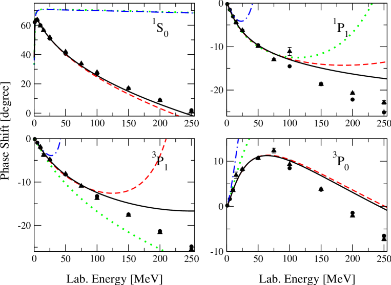
Figure 3: Phase shifts in uncoupled S- and P-waves calculated at orders $Q^{0}$ (dotted lines), $Q^{1}$ (dash-dotted lines), $Q^{2}$ (dashed lines) and $Q^{3}$ (solid lines) in comparison with the Nijmegen Stoks:1993tb (filled circles) and SAID SAID_NN (filled triangles) PWAs. Notice that the dotted and dash-dotted lines nearly coinside for the ¹S₀ phase shift.

In the ${}^{1}S_{0}$ partial wave, there is one free parameter (two free parameters) at orders $Q^{0}$ and $Q^{1}$ ($Q^{2}$ and $Q^{3}$). It is well known that an accurate description of the ${}^{1}S_{0}$ phase shift requires the inclusion of the subleading contact interaction in order to account for a rather large effective range in this channel. Our results agree with these expectation. In particular, we observe a good description of the data at orders $Q^{2}$ and $Q^{3}$, where two fit parameters are available. Interestingly, including only the first left-hand cut $4m_{N}^{2}-4M_{\pi}^{2}<s<4m_{N}^{2}-M_{\pi}^{2}$ explicitly in $U_{\rm inside}$ leads to fits of a comparable quality. On the other hand, the fit appears to be rather sensitive to the value of $g_{\pi NN}$ coupling constant. Treating it as a free parameter yields a value for $g_{\pi NN}^{2}$ which lies within $10$ percent of the empirical one if one fits the data up to $T_{lab}=100$ MeV. This difference gets even smaller if the fit is restricted to a narrower energy region around the threshold. A similar sensitivity to the value of $g_{\pi NN}$ is observed in the uncoupled P-waves of Fig. 3.

For P-waves, there are no free parameters (one free parameter) at orders $Q^{0}$ and $Q^{1}$ ($Q^{2}$ and $Q^{3}$). The calculated phase shifts at orders $Q^{0}$ and $Q^{1}$ ($Q^{1}$) in the ${}^{1}P_{1}$ (${}^{3}P_{1}$) partial wave show a steep rise already at rather low energies. This reflects the appearance of nonphysical resonances generated by solving the $N/D$ equation. These artifacts disappear at orders $Q^{2}$ and $Q^{3}$. In the ${}^{3}P_{0}$ channel we observe a large contribution of the lowest-order counter term even at low energies which agrees qualitatively with the findings of Refs. Nogga:2005hy ; Epelbaum:2012ua . Given that there is just one free parameter in each of the P-wave, the phase shifts are remarkably well reproduced at order $Q^{3}$.

We now turn to the coupled channels, see Fig. 4, and first address the convergence pattern in the ${}^{3}S_{1}$-${}^{3}D_{1}$ partial waves.

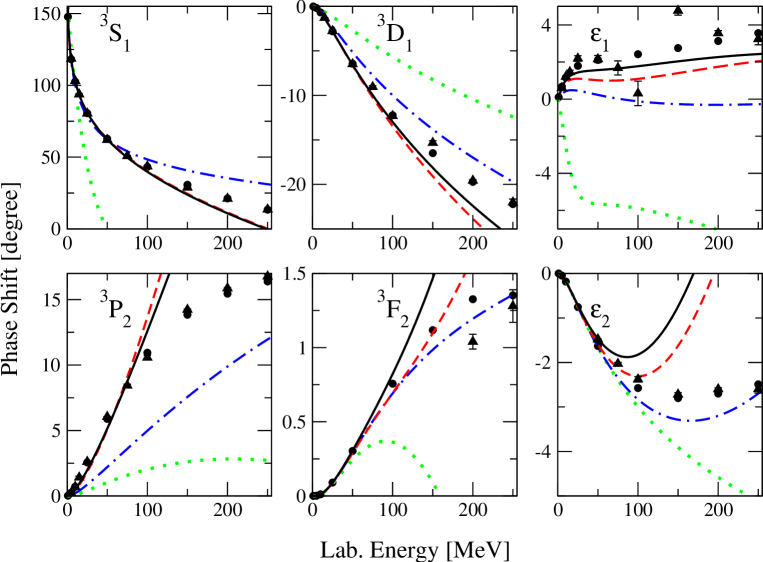
Figure 4: Phase shifts and mixing angles in the coupled ${}^{3}S_{1}$-${}^{3}D_{1}$ and ${}^{3}P_{2}$-${}^{3}F_{2}$ channels. For notation see Fig. 3.

The lowest-order (i.e. $Q^{0}$) results show a large disagreement with the empirical phase shifts. In particular, the mixing angle $\epsilon_{1}$ even comes with the wrong sign. The order-$Q^{1}$ corrections emerging from the box diagram, see Fig. 2, are large and lead to a strongly improved description of the data. Notice that there is just one free parameter at both orders $Q^{0}$ and $Q^{1}$. This suggests that the long-range physics associated with exchange of pions plays a prominent role in this channel which agrees well with the results based on chiral and phenomenological NN potentials. Taking into account the $Q^{2}$- and $Q^{3}$-contributions leads to further improvement (in part, on the cost of having two more adjustable parameters). The deuteron binding energy is also rapidly converging to its experimental value $E_{d}=-2.22$ MeV. In particular, we obtain $E_{d}=-32.70$ MeV, $-2.73$ MeV, $-2.10$ MeV and $-2.12$ MeV at orders $Q^{0}$, $Q^{1}$, $Q^{2}$ and $Q^{3}$, respectively. The situation in the ${}^{3}P_{2}$-${}^{3}F_{2}$ is qualitatively similar: one observes a large disagreement with the data at order $Q^{0}$ which is strongly reduced by taking into account the corrections at order $Q^{1}$. Notice that the results at this order are parameter-free predictions. The higher-order corrections bring our results into a better agreement with the data (on the cost of adjusting a single free parameter to the ${}^{3}P_{2}$ phase shift). The agreement with the empirical phase shifts at order $Q^{3}$ is reasonably good, especially given that there is only one adjustable parameter at this order. Note that because of the channel coupling the fit is performed simultaneously for the three phases that sometimes leads to situations when although the overall fit improves the results get worse for some particular phases when going to higher chiral order.

Apart from the counter terms, there are several parameters in our scheme whose particular values were set by physical arguments. First, the matching scale $\mu_{M}$ should, of course, be taken far away from the non-perturbative regions in the $s-$ and $t$-channels. That is why we choose $\mu_{M}$ to lie between $s$- and $t$-channel two-body thresholds. At sufficiently high order in the chiral expansion, the results should become independent on the particular choice of $\mu_{M}$ since the dependence on $\mu_{M}$ can be compensated by local NN counter terms. At order $Q^{3}$, we observe a rather week dependence on $\mu_{M}$ in most of the partial waves we have studied. For example, varying the position of $\mu_{M}$ within the region $4m_{N}^{2}-3.5M_{\pi}^{2}<\mu_{M}^{2}<4m_{N}^{2}-1.1M_{\pi}^{2}$ affects the ${}^{3}D_{1}$ phase shifts at $E_{\rm lab}=250$ MeV, where the effect is the largest, by less then 10%. The variation in the leading order is, as one can expect, stronger but does not exceed $30\%$ at $E_{\rm lab}\leq 100$ MeV. The second source of uncertainty is associated with the choice of conformal mapping and, in particular, of the value of $\Lambda_{s}$. To the order we are working, the variation of $\Lambda_{s}$ only affects the S-waves, where the expansion of $U_{\rm outside}$ goes beyond the zeroth order in $\xi$. Small variations of $\Lambda_{s}$ do not lead to sizable effects on the results. For an illustration, we show in Fig. 5 the effect of the variation of $\Lambda_{s}$ within the extremely large range $2m_{N}+M_{\pi}\leq\Lambda_{s}<\infty$.

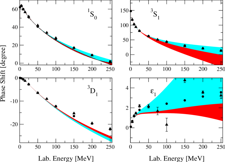
Figure 5: Sensitivity of the ${}^{1}S_{0}$ and ${}^{3}S_{1}$-${}^{3}D_{1}$ partial waves to the variation of $\Lambda_{s}$ at order $Q^{3}$. Light shaded bands correspond to the variation of $\Lambda_{s}$ in the range $2m_{N}+M_{\pi}\leq\Lambda_{s}\leq 2m_{N}+2M_{\pi}$, whereas dark shaded bands correspond to the range $2m_{N}+2M_{\pi}\leq\Lambda_{s}<\infty$.

Both limits are highly unphysical: the lower one is located very close to the energy region we are interested in and thus makes the $\xi$-expansion there unreliable while the upper one assumes the irrelevance of inelastic cuts in the whole energy region. One can see that even within these extreme limits, the variation of the phase shifts is rather modest. Only in the ${}^{3}S_{1}$ phase shift and in the mixing angle $\epsilon_{1}$ one observes a sizable variation at higher energies. Varying $\Lambda_{s}$ within a reasonable range does not affect our results in a significant way. The dependence of the results on the parameter of conformal mapping $\Lambda$ is much weaker than the dependence on $\Lambda_{s}$ and will be given in a separate publication.

We now briefly compare our results with those obtained in Refs. Albaladejo:2011bu ; Albaladejo:2012sa . Differently to these calculations, an essential ingredient of our approach is an analytic continuation of the generalized potential from the subthreshold to the physical region by means of conformal mapping which relies on a clear separation between soft and hard left hand cuts. This also allows us to avoid a sophisticated regularization procedure for the nonlinear integral equation Eq. (2) adopted in Refs. Albaladejo:2011bu ; Albaladejo:2012sa . It is difficult to carry out a more precise comparison between our approach and the one of Refs. [9,10] as those calculations are limited to LO. We, however, emphasize that the results for the uncoupled channels at LO look similar in both approaches.

5 Summary

In this work, we performed an analytic continuation of the subthreshold NN amplitude into the physical region assuming the validity of ChPT for the amplitude at some matching point below threshold. The amplitudes at the matching point and the discontinuities across the nearby left-hand cuts are calculated to order $Q^{3}$ using a manifestly covariant version of ChPT. The contributions from distant left-hand cuts are extrapolated to higher energies using conformal mapping techniques. The resulting generalized potential is used to reconstruct the full scattering amplitude by means of partial-wave dispersion relations supplemented by the unitarity constraint. Within our approach, the short-range part of the generalized potential is parametrized in a systematic way in terms of the Taylor expansion of $U_{\rm outside}(s)$ in a conformal variable $\xi(s)$. From the conceptual point of view, this is analogous to the representation of the short-range part of the nuclear force in terms of contact interactions with an increasing number of derivatives. We have determined the corresponding coefficients entering the expansion of $U_{\rm outside}(s)$ in S- and P-waves by fitting them to the Nijmegen PWA up to the energy of $T_{lab}=100$ MeV. The obtained fits and predictions for phase shifts at higher energies are in a reasonable agreement with the empirical PWAs up to $T_{lab}=250$ MeV. The quality of the fit at order $Q^{3}$ is comparable with the one obtained in conventional approaches (at next-to-next-to-leading order) based on the chiral expansion of the NN potential. In all partial waves, the expansion for the phase shifts seems to converge when going from the order $Q^{0}$ to $Q^{3}$. This supports our assumption of the validity of a perturbative expansion of the NN amplitude at the matching point. We also studied the dependence of the results on the particular choice of the matching point $\mu_{M}$ and the conformal mapping parameter $\Lambda_{s}$. We found our results to be rather weakly dependent on $\mu_{M}$ and $\Lambda_{s}$ provided these parameters are varied within a physically acceptable range.

Our detailed analysis provides new insights into the relative importance of contributions associated with the one- and two-pion exchange cuts. Such conclusions are more difficult to draw in calculations based on a potential scheme, where the left-hand cuts in the scattering amplitude emerge not only from the potential but also from its iterations within the dynamical equation. As an important outcome of our investigation, we found unambiguously that NN scattering in the ${}^{3}S_{1}-^{3}D_{1}$ channel shows a strong evidence of the lowest-order two-pion exchange which in the conventional, Schrödinger-equation-based approaches corresponds to the first iteration of the one-pion exchange potential. In particular, taking into account the leading two-pion exchange is absolutely necessary to achieve a good description of the mixing angle $\epsilon_{1}$.

Appendix A Values of the generalized potential at the matching point

The values of the generalized potential at the matching point are collected in tables 1,2, whereas derivatives of the relevant matrix elements of the generalized potential at the matching point are equal to

$${}^{1}S_{0}:\ \frac{dU(s)}{ds}{\bigg{\rvert}}_{s=\mu_{M}^{2}} = -4.57\times 10^{-3}\,\rm{MeV}^{-2}\,,$$

$${}^{3}S_{1}-^{3}D_{1}:\ \frac{dU_{11}(s)}{ds}{\bigg{\rvert}}_{s=\mu_{M}^{2}} = -1.39\times 10^{-3}\,\rm{MeV}^{-2}\,,$$

at order $Q^{2}$, and

$${}^{1}S_{0}:\ \frac{dU(s)}{ds}{\bigg{\rvert}}_{s=\mu_{M}^{2}} = -2.71\times 10^{-3}\,\rm{MeV}^{-2}\,,$$

$${}^{3}S_{1}-^{3}D_{1}:\ \frac{dU_{11}(s)}{ds}{\bigg{\rvert}}_{s=\mu_{M}^{2}} = -1.45\times 10^{-3}\,\rm{MeV}^{-2}\,,$$

at order $Q^{3}$. One-pion-exchange contributions are always subtracted.

	${}^{1}S_{0}$	${}^{1}P_{1}$	${}^{3}P_{1}$	${}^{3}P_{0}$
$Q^{0}$	$5.79\times 10^{2}$
$Q^{1}$	$5.82\times 10^{2}$
$Q^{2}$	$8.53\times 10^{2}$	$1.42\times 10^{3}$	$3.46\times 10^{3}$	$-6.43\times 10^{3}$
$Q^{3}$	$8.63\times 10^{2}$	$2.19\times 10^{3}$	$4.81\times 10^{3}$	$-5.70\times 10^{3}$

Table 1: Generalized potential at the matching point $U(\mu_{M}^{2})$ that contain adjusted parameters at different chiral orders after subtracting one-pion exchange contribution. Uncoupled partial waves.

	${}^{3}S_{1}-^{3}D_{1}\,,\,U_{11}$	${}^{3}S_{1}-^{3}D_{1}\,,\,U_{12}$	${}^{3}P_{2}-^{3}D_{2}\,,\,U_{11}$
$Q^{0}$	$-2.95\times 10^{2}$
$Q^{1}$	$6.14\times 10^{2}$
$Q^{2}$	$2.08\times 10^{2}$	$-5.92\times 10^{3}$	$5.59\times 10^{2}$
$Q^{3}$	$2.07\times 10^{2}$	$-6.94\times 10^{3}$	$7.50\times 10^{2}$

Table 2: Matrix elements of the generalized potential at the matching point $U_{ij}(\mu_{M}^{2})$ that contain adjusted parameters at different chiral orders after subtracting one-pion exchange contribution. Coupled partial waves.

References

- (1) S. Weinberg, Nucl. Phys. B363, 3 (1991)
- (2) C. Ordonez, U. van Kolck, Phys.Lett. B291, 459 (1992)
- (3) D. Entem, R. Machleidt, Phys.Rev. C68, 041001 (2003), nucl-th/0304018
- (4) E. Epelbaum, W. Glöckle, U.-G. Meißner, Nucl.Phys. A747, 362 (2005), nucl-th/0405048
- (5) E. Epelbaum, H.-W. Hammer, U.-G. Meißner, Rev.Mod.Phys. 81, 1773 (2009), 0811.1338
- (6) R. Machleidt, D. Entem, Phys.Rept. 503, 1 (2011), 1105.2919
- (7) M. Goldberger, M. T. Grisaru, S. MacDowell, et al., Phys.Rev. 120, 2250 (1960)
- (8) J. S. Ball, A. Scotti, D. Y. Wong, Phys.Rev. 142, 1000 (1966)
- (9) A. Scotti, D. Wong, Phys.Rev.Lett. 10, 142 (1963)
- (10) A. Scotti, D. Wong, Phys.Rev. 138, B145 (1965)
- (11) M. Albaladejo, J. Oller, Phys.Rev. C84, 054009 (2011), 1107.3035
- (12) M. Albaladejo, J. Oller, Phys.Rev. C86, 034005 (2012), 1201.0443
- (13) A. Gasparyan, M. F. M. Lutz, Nucl.Phys. A848, 126 (2010), 1003.3426
- (14) A. Gasparyan, M. Lutz, Fizika B20, 55 (2011), 1012.5948
- (15) A. Gasparyan, M. Lutz, B. Pasquini, Nucl.Phys. A866, 79 (2011), 1102.3375
- (16) C. Ditsche, M. Hoferichter, B. Kubis, et al., JHEP 1206, 043 (2012), 1203.4758
- (17) I. Danilkin, L. Gil, M. Lutz, Phys.Lett. B703, 504 (2011), 1106.2230
- (18) I. Danilkin, M. Lutz, S. Leupold, et al., Eur.Phys.J. C73, 2358 (2013), 1211.1503
- (19) M. Rentmeester, R. Timmermans, J. L. Friar, et al., Phys.Rev.Lett. 82, 4992 (1999), nucl-th/9901054
- (20) M. C. Birse, J. A. McGovern, Phys.Rev. C70, 054002 (2004), nucl-th/0307050
- (21) M. C. M. Rentmeester, R. G. E. Timmermans, J. J. de Swart, Phys. Rev. C67, 044001 (2003), nucl-th/0302080
- (22) M. C. Birse, Phys.Rev. C76, 034002 (2007), 0706.0984
- (23) D. Shukla, D. R. Phillips, E. Mortenson, J.Phys. G35, 115009 (2008), 0803.4190
- (24) M. C. Birse, Eur.Phys.J. A46, 231 (2010), 1007.0540
- (25) D. B. Kaplan, M. J. Savage, M. B. Wise, Nucl.Phys. B478, 629 (1996), nucl-th/9605002
- (26) G. Lepage 135–180 (1997), nucl-th/9706029
- (27) S. Beane, P. F. Bedaque, M. Savage, et al., Nucl.Phys. A700, 377 (2002), nucl-th/0104030
- (28) A. Nogga, R. Timmermans, U. van Kolck, Phys.Rev. C72, 054006 (2005), nucl-th/0506005
- (29) M. C. Birse, Phys.Rev. C74, 014003 (2006), nucl-th/0507077
- (30) M. Pavon Valderrama, E. Ruiz Arriola, Phys.Rev. C74, 054001 (2006), nucl-th/0506047
- (31) E. Epelbaum, U.-G. Meißner (2006), nucl-th/0609037
- (32) B. Long, C. Yang, Phys.Rev. C85, 034002 (2012), 1111.3993
- (33) I. Danilkin, A. Gasparyan, M. Lutz, Phys.Lett. B697, 147 (2011), 1009.5928
- (34) G. F. Chew, S. Mandelstam, Phys. Rev. 119, 467 (1960)
- (35) S. Stoica, M. Lutz, O. Scholten, Phys.Rev. D84, 125001 (2011), 1106.5619
- (36) H. Stapp, T. Ypsilantis, N. Metropolis, Phys.Rev. 105, 302 (1957)
- (37) N. Fettes, U.-G. Meißner, S. Steininger, Nucl. Phys. A640, 199 (1998), hep-ph/9803266
- (38) N. Fettes, U.-G. Meißner, M. Mojzis, et al., Annals Phys. 283, 273 (2000), hep-ph/0001308
- (39) M. Lutz, Nucl.Phys. A677, 241 (2000), nucl-th/9906028
- (40) R. Higa, M. Robilotta, Phys.Rev. C68, 024004 (2003), nucl-th/0304025
- (41) G. Passarino, M. Veltman, Nucl.Phys. B160, 151 (1979)
- (42) A. Semke, M. Lutz, Nucl.Phys. A778, 153 (2006), nucl-th/0511061
- (43) T. Fuchs, J. Gegelia, G. Japaridze, et al., Phys.Rev. D68, 056005 (2003), hep-ph/0302117
- (44) N. Kaiser, R. Brockmann, W. Weise, Nucl.Phys. A625, 758 (1997), nucl-th/9706045
- (45) J. L. Friar, Phys.Rev. C60, 034002 (1999), nucl-th/9901082
- (46) R. G. E. Timmermans, T. A. Rijken, J. J. de Swart, Phys. Rev. Lett. 67, 1074 (1991)
- (47) V. Baru, C. Hanhart, M. Hoferichter, et al., Phys.Lett. B694, 473 (2011), 1003.4444
- (48) J. L. Friar, U. van Kolck, G. Payne, et al., Phys.Rev. C68, 024003 (2003), nucl-th/0303058
- (49) H. Krebs, A. Gasparyan, E. Epelbaum, Phys.Rev. C85, 054006 (2012), 1203.0067
- (50) E. Epelbaum, W. Gloeckle, U.-G. Meissner, Eur.Phys.J. A19, 125 (2004), nucl-th/0304037
- (51) E. Epelbaum, W. Gloeckle, U.-G. Meissner, Eur.Phys.J. A19, 401 (2004), nucl-th/0308010
- (52) V. Bernard, N. Kaiser, U.-G. Meißner, Nucl. Phys. A615, 483 (1997), hep-ph/9611253
- (53) V. Stoks, R. Kompl, M. Rentmeester, et al., Phys.Rev. C48, 792 (1993)
- (54) L. Girlanda, M. Viviani, Few Body Syst. 49, 51 (2011)
- (55) N. A. Arndt, et al., SAID online program, http://gwdac.phys.gwu.edu
- (56) E. Epelbaum, J. Gegelia, Phys.Lett. B716, 338 (2012), 1207.2420