Quark disconnected diagrams in chiral perturbation theory - the scalar form factor

Abstract:

Expressions for the Wick contractions contributing to the scalar pion form-factor were computed model-independently in chiral perturbation theory at next-to-leading order. The results reveal correlations amongst the different contractions in terms of low-energy constants and allow for extrapolating lattice data for individual Wick contractions. The quark disconnected contribution to the real part of the form factor turns out to be suppressed with respect to the quark connected one. The corresponding contribution to the scalar radius has the same size as the connected contribution and can therefore not be neglected.

1 Introduction

Quark disconnected Wick contractions constitute a considerable numerical problem for lattice QCD. An estimate of the full quark-propagator is needed and the signal-to-noise ratio typically leaves a lot to be desired. In current simulations in the iso-spin symmetric limit disconnected contractions contribute to a number of phenomenologically relevant quantities ($g-2$, $\pi\pi$-scattering, hadronic $K$-decays, …). The situation becomes worse once also iso-spin breaking effects are included in the simulations since disconnected contributions will then contribute in a larger variety and to many more quantities.

Given the difficulties in computing quark disconnected contractions to a satisfactory precision in lattice simulations one often neglects them, thereby introducing an unknown systematic effect. Large efforts therefore go into devising dedicated algorithms for improving the numerical evaluation of quark-disconnected diagrams (e.g. [3, 4, 2]). Here, an analytical and model-independent approach for computing individual Wick contractions in chiral perturbation theory which was presented in [5] is applied to the case of the scalar pion form factor [6] for QCD with $N_{f}=2$ and $N_{f}=2+1$ dynamical flavours. At next-to-leading order (NLO) in the chiral expansion the contribution of the disconnected contraction to the form-factor is numerically small. Both the disconnected and the connected contribution however contribute with roughly the same magnitude to the scalar radius. The connected and disconnected contributions turn out to be correlated in terms of low-energy constants of the chiral Lagrangian. The expressions derived here can be used to guide chiral extrapolations of lattice results for individual Wick contractions. As an aside the argument allowing to compute the quark-connected part with partially twisted boundary conditions [7, 8] for an improved momentum resolution for the scalar form factor is presented.

2 Technique

The scalar form factor of the pion is defined as

$$\langle\pi^{i}(p^{\prime})|\bar{u}u+\bar{d}d|\pi^{j}(p)\rangle=\delta^{ij}F_{S,2}(t)\,,$$ (1)

where $t=(p^{\prime}-p)^{2}$ is the squared momentum transfer between the initial and final pion and the sub-script on the r.h.s. identifies the scalar form factor for $N_{f}=2$ flavour QCD. In lattice QCD the matrix element on the l.h.s. is computed in terms of the ground-state contribution to the Fourier transform of the Euclidean 3-pt. function

$$\left<{O}^{i}(z)S(y){{O}^{i}}^{\dagger}(x)\right>\,,$$ (2)

constructed of the interpolating operators $O^{i}(x)=\bar{\psi}_{2}\tau^{i}\gamma_{5}\psi_{2}(x)$ and $S(x)=\bar{\psi}_{2}(x)\psi_{2}(x)$. The $\psi^{T}_{2}=(u,d)$ are $SU(2)$ flavour vectors of $u$- and $d$-quarks and the matrices $\tau_{i}=\sigma_{i}/2$ are proportional to the Pauli matrices. Following [5] the two types of Wick contractions contributing to this correlation function are

$$\langle\bar{u}\gamma_{5}d\,\bar{d}d\,\bar{d}\gamma_{5}u\rangle=\langle\bar{u}\gamma_{5}v\,\bar{v}d\,\bar{d}\gamma_{5}u\rangle+\langle\bar{u}\gamma_{5}d\,\bar{v}v\,\bar{d}\gamma_{5}u\rangle\,.$$ (3)

Note the additional valence quark $v$ with $m_{u}=m_{d}=m_{v}$ that was introduced in order to construct the decomposition on the r.h.s.. At this stage the connected contribution consists entirely of flavour off-diagonal currents and the argument presented in [9, 5] allows to compute at least this contribution using partially twisted boundary conditions, thus improving the momentum resolution. Each individual term on the r.h.s. represents an unphysical correlation function in the unphysical theory, QCD with an additional valence quark $v$. The expression in chiral effective theory for the ground state contribution to the l.h.s. has been derived many years ago in chiral perturbation theory at NLO [10, 11] and later at NNLO [12, 13] in both $SU(2)$ and $SU(3)$ chiral perturbation theory. The effective theory frame work for the computation of the corresponding contributions to the r.h.s. is partially quenched chiral perturbation theory (PQ$\chi$PT) [14, 15] which is a frame-work allowing to vary the sea-quark and valence-quark content independently. While the individual terms on the r.h.s. represent unphysical matrix elements, their sum represents a physical process. It is therefore conceivable to use different methods for the computation of the terms on the r.h.s.. The connected contribution is conveniently computed in a lattice simulation. Where the disconnected contribution is difficult to compute numerically the method advocated here can be applied.

3 PQ$\chi$PT for the scalar form factor

According to [14, 15] the chiral effective theory for $N_{f}=2$ and $N_{f}=2+1$ QCD with an additional valence quark $v$ is developed around the graded flavour symmetry groups $SU(3|1)$ and $SU(4|1)$, respectively. The leading order chiral Lagrangian is [10, 14, 15, 16, 17]

$$\mathcal{L}^{(2)}=\frac{F^{2}}{4}{\rm Str}\left\{\partial_{\mu}U\partial^{\mu}U^{\dagger}\right\}+\frac{F^{2}}{4}{\rm Str}\left\{\chi U^{\dagger}+U\chi^{\dagger}\right\}\,,$$ (4)

where $\chi=2B(s+M)$. The mass matrix has the form $M={\rm diag}\left(m_{q},m_{q},m_{q},m_{q}\right)$ in $SU(3|1)$ and $M={\rm diag}\left(m_{q},m_{q},m_{s},m_{q},m_{q}\right)$ in $SU(4|1)$ and we define the external scalar source as $s=2T^{a}s^{a}$ (with $T^{a}$ a generator of the flavour group). The relevant counter terms can be derived from the Lagrangian,

$$\begin{array}[]{rcl}\mathcal{L}^{(4)}&=&L_{4}{\rm Str}\Big{\{}\partial_{\mu}U(\partial^{\mu}U)^{\dagger}\Big{\}}{\rm Str}\Big{\{}\chi U^{\dagger}+U\chi^{\dagger}\Big{\}}+L_{5}{\rm Str}\Big{\{}\big{(}\partial_{\mu}U(\partial^{\mu}U)^{\dagger}\big{)}\big{(}\chi U^{\dagger}+U\chi^{\dagger}\big{)}\Big{\}}\\[5.69054pt] &&+L_{6}{\rm Str}\Big{\{}\chi U^{\dagger}+U\chi^{\dagger}\Big{\}}^{2}+L_{8}{\rm Str}\Big{\{}U\chi^{\dagger}U\chi^{\dagger}+\chi U^{\dagger}\chi U^{\dagger}\Big{\}}^{2}\,.\end{array}$$ (5)

The remaining calculation proceeds as in standard chiral perturbation theory. The known result for the full form factor is reproduced,

$$F^{\rm F}_{S,2}(t) = 2B\Big{\{}1+\frac{1}{F^{2}}\Big{(}-\frac{1}{2}{\bar{A}}_{m_{\pi}^{2}}\hskip 36.98857pt+\,\Lambda^{\rm F}_{2}\hskip 65.44133pt+\frac{(2t-\;\,{m_{\pi}^{2}})}{2}{\bar{B}}({m_{\pi}^{2}},t)\Big{)}\Big{\}}\,,$$ (6)

$$F_{S,3}^{{\rm F}}(t) = 2B\Big{\{}1+\frac{1}{F^{2}}\Big{(}-\frac{1}{2}{\bar{A}}_{m_{\pi}^{2}}+\frac{1}{6}{\bar{A}}_{m_{\eta}^{2}}+\,\Lambda_{3}^{{\rm F}}+\frac{{m_{\pi}^{2}}}{18}{\bar{B}}({m_{\eta}^{2}},t)+\frac{(2t\,\,-{{m_{\pi}^{2}}})}{2}{\bar{B}}({m_{\pi}^{2}},t)+\frac{t}{4}{\bar{B}}({m_{K}^{2}},t)\Big{)}\Big{\}}\,.$$

The expressions for $\bar{A}_{m^{2}}$ and $\bar{B}(m^{2},t)$ are standard and can be found in [6]. The new results are the individual expression for the connected ($F^{C}_{S,N_{f}}$) and disconnected contribution ($F^{C}_{S,N_{f}}$):

$$F^{\rm C}_{S,2}(t) = 2B\Big{\{}1+\frac{1}{F^{2}}\Big{(}-\frac{1}{2}{\bar{A}}_{m_{\pi}^{2}}\hskip 34.1433pt+\Lambda^{\rm C}_{2}+\frac{(t-2{m_{\pi}^{2}})}{2}{\bar{B}}({m_{\pi}^{2}},t)\Big{)}\Big{\}}\,,$$

$$F^{\rm D}_{S,2}(t) = 2B\Big{\{}0+\frac{1}{F^{2}}\Big{(}\hskip 68.2866pt+\Lambda^{\rm D}_{2}+\frac{(t+\;\,{m_{\pi}^{2}})}{2}{\bar{B}}({m_{\pi}^{2}},t)\Big{)}\Big{\}}\,,$$ (7)

$$F_{S,3}^{{\rm C}}(t) = 2B\Big{\{}1+\frac{1}{F^{2}}\Big{(}-\frac{1}{2}{\bar{A}}_{m_{\pi}^{2}}+\frac{1}{6}{\bar{A}}_{m_{\eta}^{2}}+\Lambda_{3}^{{\rm C}}+\frac{(t-2{m_{\pi}^{2}})}{2}{\bar{B}}({m_{\pi}^{2}},t)+\frac{t}{4}{\bar{B}}({m_{K}^{2}},t)+\frac{{m_{\pi}^{2}}}{3}{\bar{B}}({m_{\eta}^{2}},{m_{\pi}^{2}},t)\Big{)}\Big{\}}\,,$$

$$F_{S,3}^{{\rm D}}(t) = 2B\Big{\{}0+\frac{1}{F^{2}}\Big{(}\hskip 68.2866pt+\Lambda_{3}^{{\rm D}}+\frac{(t+\;\,{m_{\pi}^{2}})}{2}{\bar{B}}({m_{\pi}^{2}},t)+\frac{{m_{\pi}^{2}}}{18}{\bar{B}}({m_{\eta}^{2}},t)-\frac{{m_{\pi}^{2}}}{3}{\bar{B}}({m_{\eta}^{2}},{m_{\pi}^{2}},t)\Big{)}\Big{\}}\,.$$

Note that for both $N_{f}=2$ and $N_{f}=2+1$, $F_{S}^{F}=F_{S}^{C}+F_{S}^{D}$, as expected. The $\Lambda_{N_{f}}^{C/D}$ contain combinations of the low energy constants (LECs),

$$\begin{array}[]{l@{\hspace{1mm}}c@{\hspace{1mm}}l@{\hspace{0mm}}l@{\hspace{0mm}}l@{\hspace{0mm}}l@{\hspace{0mm}}l@{\hspace{0mm}}l@{\hspace{0mm}}l@{\hspace{0mm}}}\Lambda_{2}^{{\rm F}}\hfil\hskip 2.84526pt&=\hfil\hskip 2.84526pt&4\Big{\{}{m_{\pi}^{2}}(-8\tilde{L}_{4}^{r}-4\tilde{L}_{5}^{r}&+16\tilde{L}_{6}^{r}&+8\tilde{L}_{8}^{r})&+t(2\tilde{L}_{4}^{r}+\tilde{L}_{5}^{r})&\Big{\}}\,,\\[8.53581pt] \Lambda_{2}^{{\rm C}}\hfil\hskip 2.84526pt&=\hfil\hskip 2.84526pt&4\Big{\{}{m_{\pi}^{2}}(-4\tilde{L}_{4}^{r}-4\tilde{L}_{5}^{r}&+8\tilde{L}_{6}^{r}&+8\tilde{L}_{8}^{r})&+t\hskip 35.56593pt\tilde{L}_{5}^{r}&\Big{\}}\,,\\[8.53581pt] \Lambda_{2}^{{\rm D}}\hfil\hskip 2.84526pt&=\hfil\hskip 2.84526pt&4\Big{\{}{m_{\pi}^{2}}(-4\tilde{L}_{4}^{r}&+8\tilde{L}_{6}^{r})&&+t\;\,2\tilde{L}_{4}^{r}&\Big{\}}\,,\end{array}$$ (8)

and

$$\begin{array}[]{l@{\hspace{1mm}}c@{\hspace{1mm}}l@{\hspace{0mm}}l@{\hspace{0mm}}l@{\hspace{0mm}}l@{\hspace{0mm}}l@{\hspace{0mm}}l@{\hspace{0mm}}l@{\hspace{0mm}}}\Lambda_{3}^{{\rm F}}\hfil\hskip 2.84526pt&=\hfil\hskip 2.84526pt&4\Big{\{}{m_{\pi}^{2}}(-6L_{4}^{r}-4L_{5}^{r}&+12L_{6}^{r}&+8L_{8}^{r})&+{m_{K}^{2}}(-4L_{4}^{r}+8L_{6}^{r})&+t(2L_{4}^{r}+L_{5}^{r})&\Big{\}}\,,\\[8.53581pt] \Lambda_{3}^{{\rm C}}\hfil\hskip 2.84526pt&=\hfil\hskip 2.84526pt&4\Big{\{}{m_{\pi}^{2}}(-2L_{4}^{r}-4L_{5}^{r}&+4L_{6}^{r}&+8L_{8}^{r})&+{m_{K}^{2}}(-4L_{4}^{r}+8L_{6}^{r})&+t\hskip 35.56593ptL_{5}^{r}&\Big{\}}\,,\\[8.53581pt] \Lambda_{3}^{{\rm D}}\hfil\hskip 2.84526pt&=\hfil\hskip 2.84526pt&4\Big{\{}{m_{\pi}^{2}}(-4L_{4}^{r}&+8L_{6}^{r})&&&+t\;\,2L_{4}^{r}&\Big{\}}\,.\end{array}$$ (9)

The $L_{i}^{r}$ are the LECs of $SU(3)$ chiral perturbation theory [16] and the $\tilde{L}_{i}^{r}$ are related to the better-known $SU(2)$ LECs $l_{i}^{r}$ via matching,

$$\begin{array}[]{l@{\hspace{1mm}}c@{\hspace{1mm}}l@{\hspace{0mm}}l@{\hspace{0mm}}l@{\hspace{0mm}}l@{\hspace{0mm}}l@{\hspace{0mm}}l@{\hspace{0mm}}l@{\hspace{0mm}}l@{\hspace{0mm}}}\Lambda^{\rm F}_{2}\hfil\hskip 2.84526pt&=\hfil\hskip 2.84526pt&t\;\,l_{4}^{r}&&+4{m_{\pi}^{2}}\;\,l_{3}^{r}\,,\\[8.53581pt] \Lambda^{\rm C}_{2}\hfil\hskip 2.84526pt&=\hfil\hskip 2.84526pt&t(l_{4}^{r}&-8\tilde{L}_{4}^{r})&+4{m_{\pi}^{2}}(l_{3}^{r}&+4\tilde{L}_{4}^{r}&-8\tilde{L}_{6}^{r})\,,\\[8.53581pt] \Lambda^{\rm D}_{2}\hfil\hskip 2.84526pt&=\hfil\hskip 2.84526pt&t(&+8\tilde{L}_{4}^{r})&+4{m_{\pi}^{2}}(&-4\tilde{L}_{4}^{r}&+8\tilde{L}_{6}^{r})\,.\end{array}$$ (10)

The remaining $SU(3|1)$ constants $\tilde{L}_{4}^{r}$ and $\tilde{L}_{6}^{r}$ are less well known since the corresponding terms in the $L^{(4)}$-Lagrangian can be removed in the case of the flavour group $SU(2)$ (trace-identities). For $N_{f}=2+1$ similar expressions for the individual Wick contractions can be derived for the octet and singlet form form factors

$$\begin{array}[]{lcl}\langle\pi^{i}|\bar{u}u+\bar{d}d-2\bar{s}s|\pi^{k}\rangle&=&\delta^{ik}F_{S}^{8}(t)\,,\\[8.53581pt] \langle\pi^{i}|\bar{u}u+\bar{d}d+\bar{s}s|\pi^{k}\rangle&=&\delta^{ik}F_{S}^{0}(t)\,.\\[8.53581pt] \end{array}$$ (11)

From the expressions in eq. (3) we see that while the connected contribution to the form factor starts at leading order, the disconnected contribution starts at NLO and is therefore expected to be smaller in magnitude. Turning to the scalar radius $\langle r^{2}\rangle=6\frac{dF_{S}(t)}{dt}|_{t=0}$, the derivative with respect to the momentum removes the leading term from the connected contribution and therefore connected and disconnected contribution start contributing at the same order in the chiral power counting.

Concentrating on the $N_{f}=2+1$-case we now fix the free parameters in the expression for $F_{S,3}^{F/C/D}(t)$ with input as summarised in table 1. The results for the 2-flavour case, which turn out to be very similar both qualitatively and quantitatively, can be obtained after fixing the $\tilde{L}^{r}_{i}$ through matching the unphysical LECs to the 3-flavour theory [6].

$L_{4}^{r}$	[18, 19]	$0.14\times 10^{-3}$
$L_{5}^{r}$	[18, 19]	$0.87\times 10^{-3}$
$L_{6}^{r}$	[18, 19]	$0.07\times 10^{-3}$
$L_{8}^{r}$	[18, 19]	$0.56\times 10^{-3}$

Table 1: Values for the 3-flavour low energy constants used in the illustration of the results. The subtraction scale is $\mu=0.77$GeV.

The results are shown in the plots in figure 1 for the full form factor and the connected and disconnected contribution, respectively. For the real part the magnitude of the disconnected contribution is sub-dominant in line with the above observations. Above the two-pion threshold the disconnected contribution also contributes to the imaginary part and is similar in magnitude to the connected contribution. Since the leading contribution has no imaginary part this does not come as a surprise - the imaginary part in both the connected and the disconnected contribution start at the same order, NLO. We also show the mass-dependence of the scalar radius. What could have been anticipated from the first of the three plots by observing that the slope around $t=0$ of the connected and disconnected contribution is very similar, is confirmed in the third plot - the connected and disconnected contributions to the scalar radius are nearly of the same size. For a lattice simulation this underlines that the disconnected contribution cannot be neglected [1, 2].

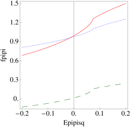
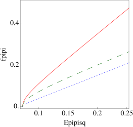
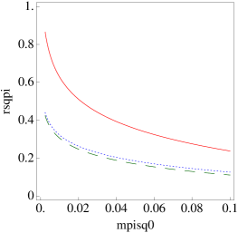
Figure 1: First row: the plots show the momentum dependence of the real (left) and imaginary (right) parts of the scalar form factor for $N_{f}=2+1$: Full form factor (solid red), connected contribution (dotted blue) and disconnected contribution (dashed green). The bottom plot shows the scalar radius for $N_{f}=2+1$ as a function of the squared pion mass ($m_{K}$ is fixed to the physical value and ${m_{\eta}^{2}}=\frac{4}{3}{m_{K}^{2}}-\frac{1}{3}{m_{\pi}^{2}}$, same color coding as first row).

4 Conclusion

Partially quenched chiral perturbation theory proves to be a powerful tool for understanding in detail the dynamics in the low-energy sector of QCD. The decomposition of correlation functions into individual Wick contractions provides guidance for lattice computations in various ways: First of all an estimate of the magnitude of the disconnected contribution can be made in a model-independent way. Secondly, NLO LECs can be extracted from only the connected contribution to the form factor which is numerically much better accessible in lattice simulations. The expression does however contain new linear combinations of LECs and one has to study whether the LEC one is interested in can be extracted. Thirdly, a full computation of the form factor in lattice QCD is still very challenging due to the numerical cost of computing the disconnected contribution to a satisfactory precision. In this situation one can either compute only the connected contribution in lattice QCD and predict the disconnected one, or one computes the connected contribution for a large set of parameters, while the disconnected one only for a reduced set of parameters to fix the LECs and to eventually extrapolate it to the physical point.

Acknowledgements: The research leading to these results has received funding from the European Research Council under the European Union’s Seventh Framework Programme (FP7/2007-2013) / ERC Grant agreement 279757.

References

- [1] JLQCD Collaboration, TWQCD Collaboration Collaboration, S. Aoki et. al., Pion form factors from two-flavor lattice QCD with exact chiral symmetry, Phys.Rev. D80 (2009) 034508, [0905.2465].
- [2] V. Gülpers, G. von Hippel, and H. Wittig, The scalar Pion Form Factor with Wilson fermions, PoS LATTICE2012 (2012) 181.
- [3] J. Foley et. al., Practical all-to-all propagators for lattice QCD, Comput. Phys. Commun. 172 (2005) 145–162, [hep-lat/0505023].
- [4] G. S. Bali, S. Collins, and A. Schafer, Effective noise reduction techniques for disconnected loops in Lattice QCD, Comput.Phys.Commun. 181 (2010) 1570–1583, [0910.3970].
- [5] M. Della Morte and A. Jüttner, Quark disconnected diagrams in chiral perturbation theory, JHEP 1011 (2010) 154, [1009.3783].
- [6] A. Jüttner, Revisiting the pion’s scalar form factor in chiral perturbation theory, JHEP 1201 (2012) 007, [1110.4859].
- [7] P. F. Bedaque, Aharonov-Bohm effect and nucleon nucleon phase shifts on the lattice, Phys.Lett. B593 (2004) 82–88, [nucl-th/0402051].
- [8] C. Sachrajda and G. Villadoro, Twisted boundary conditions in lattice simulations, Phys.Lett. B609 (2005) 73–85, [hep-lat/0411033].
- [9] P. Boyle, J. Flynn, A. Jüttner, C. Kelly, H. de Lima, et. al., The Pion’s electromagnetic form-factor at small momentum transfer in full lattice QCD, JHEP 0807 (2008) 112, [arXiv:0804.3971].
- [10] J. Gasser and H. Leutwyler, Chiral Perturbation Theory to One Loop, Ann. Phys. 158 (1984) 142.
- [11] J. Gasser and H. Leutwyler, Low-Energy Expansion of Meson Form-Factors, Nucl.Phys. B250 (1985) 517–538.
- [12] J. Bijnens, G. Colangelo, and P. Talavera, The Vector and scalar form-factors of the pion to two loops, JHEP 9805 (1998) 014, [hep-ph/9805389].
- [13] J. Bijnens and P. Dhonte, Scalar form-factors in SU(3) chiral perturbation theory, JHEP 0310 (2003) 061, [hep-ph/0307044].
- [14] C. W. Bernard and M. F. L. Golterman, Chiral perturbation theory for the quenched approximation of QCD, Phys. Rev. D46 (1992) 853–857, [hep-lat/9204007].
- [15] S. R. Sharpe and N. Shoresh, Physical results from unphysical simulations, Phys. Rev. D62 (2000) 094503, [hep-lat/0006017].
- [16] J. Gasser and H. Leutwyler, Chiral Perturbation Theory: Expansions in the Mass of the Strange Quark, Nucl. Phys. B250 (1985) 465.
- [17] C. W. Bernard and M. F. Golterman, Partially quenched gauge theories and an application to staggered fermions, Phys.Rev. D49 (1994) 486–494, [hep-lat/9306005].
- [18] RBC-UKQCD Collaboration, C. Allton et. al., Physical Results from 2+1 Flavor Domain Wall QCD and SU(2) Chiral Perturbation Theory, Phys.Rev. D78 (2008) 114509, [arXiv:0804.0473].
- [19] G. Colangelo, S. Dürr, A. Jüttner, L. Lellouch, H. Leutwyler, et. al., Review of lattice results concerning low energy particle physics, Eur.Phys.J. C71 (2011) 1695, [1011.4408].