Coagulation kinetics beyond mean field theory using an optimised Poisson representation

Abstract

Binary particle coagulation can be modelled as the repeated random process of the combination of two particles to form a third. The kinetics may be represented by population rate equations based on a mean field assumption, according to which the rate of aggregation is taken to be proportional to the product of the mean populations of the two participants, but this can be a poor approximation when the mean populations are small. However, using the Poisson representation it is possible to derive a set of rate equations that go beyond mean field theory, describing pseudo-populations that are continuous, noisy and complex, but where averaging over the noise and initial conditions gives the mean of the physical population. Such an approach is explored for the simple case of a size-independent rate of coagulation between particles. Analytical results are compared with numerical computations and with results derived by other means. In the numerical work we encounter instabilities that can be eliminated using a suitable ‘gauge’ transformation of the problem [P. D. Drummond, Eur. Phys. J. B38, 617 (2004)] which we show to be equivalent to the application of the Cameron-Martin-Girsanov formula describing a shift in a probability measure. The cost of such a procedure is to introduce additional statistical noise into the numerical results, but we identify an optimised gauge transformation where this difficulty is minimal for the main properties of interest. For more complicated systems, such an approach is likely to be computationally cheaper than Monte Carlo simulation.

I Introduction

The process of coagulation or aggregation is responsible for the coarsening of a size distribution of particles suspended in gaseous or liquid media. The phenomenon consists of a sequence of statistically independent events where two (or possibly more) particles unite, perhaps as a result of collision, to create a composite particle, and each event reduces the number of particles in the system Smoluchowski (1906); Leyvraz (2003); Lushnikov (2006). This has practical consequences such as colloidal precipitation or accelerated rainfall from clouds Pruppacher and Klett (1997); Mehlig and Wilkinson (2004); McGraw and Liu (2006). Fragmentation can take place as well Spicer and Pratsinis (1996), but precipitation processes are typically dominated by irreversible agglomeration. The phenomenon is familiar and yet it can present some surprises, an example of which was presented by Lushnikov Lushnikov (1978) in an exact study of coagulation kinetics driven by various choices of aggregation rates. He showed that in the later stages of a process where the binary coagulation rate is proportional to the product of the masses of the participants, a single particle emerges with a mass representing a sizable fraction of that of the entire system Lushnikov (2005). This has been termed a gelation event and standard kinetic models of coagulation are unable to account for the phenomenon, for the simple reason that they are designed to describe systems consisting of very large populations of particles in each size class. They rely on a mean field approximation, though this is not always clearly recognised. When small particle populations play a key role in the kinetics, different approaches become necessary Krug (2003), the most common being Monte Carlo modelling Smith and Matsoukas (1998), though analytic treatments are sometimes possible Hendriks et al. (1985).

This paper investigates the utility of a rate equation model of kinetic processes that is able to capture small population effects. The Markovian master equations that describe coagulation may be transformed mathematically into a problem in the dynamics of continuous stochastic variables acted upon by complex noise, the solution to which may be related to the evolving statistical properties of the populations in the physical system. The recasting of the problem into one that concerns complex ‘pseudo-populations’ can be done in two distinct ways, either using methods of operator algebra similar to those employed in quantum field theories Doi (1976a, b); Peliti (1985); Patzlaff et al. (1994); Rey and Droz (1997); Mattis and Glasser (1998); Sasai and Wolynes (2003); Täuber et al. (2005); Ohkubo (2007a); Schulz (2008); Ohkubo (2007b), or through the so-called Poisson representation of the populations Gardiner and Chaturvedi (1977); Gardiner (2009); Drummond (2004); Drummond et al. (2010). The physical problem concerning the stochastic evolution of a set of (integer-valued) populations is replaced by the task of solving and averaging a set of stochastic differential equations Deloubrière et al. (2002); Hochberg et al. (2006). The purpose of this paper is to explore the use of the Poisson representation in this area.

The advantage of such a transformation over Monte Carlo simulation of the process Gillespie (1977); Smith and Matsoukas (1998) emerges for cases where the particles come in many species or sizes, since the configuration space of the populations, and hence the computational cost, increases very rapidly, but in order to illustrate the approach we study a very simple example of coagulation, where the aggregation rates do not depend on the masses of the participants. This is very different from the cases that exhibit gelation, studied by Lushnikov Lushnikov (1978) and others Hendriks et al. (1985), and we might not expect major deviations from a mean field approach, but nevertheless it is possible to use the system to demonstrate the analytic procedure, and compare the accuracy of numerical pseudo-population dynamics and averaging with respect to other approaches Barzykin and Tachiya (2005); Biham and Furman (2001); Lushnikov et al. (2003); Bhatt and Ford (2003); Green et al. (2001); Losert-Valiente Kroon and Ford (2007), in order to form a view on the usefulness of the approach. We do not suggest that such a method is to be preferred over others for such simple examples, since the technique is much more elaborate. There might, nevertheless, be cases where the approach might have analytic advantages even where mean field equations are largely adequate, and the area of nucleation modelling and barrier crossing is one worth exploring Bhatt and Ford (2003); Yvinec et al. (2012).

In Section II the master equations describing the basic problem of $A+A\to A$ aggregation are developed and the Poisson representation is introduced and used to derive the equivalent stochastic dynamics problem and associated averaging scheme. The evolving complex pseudo-population is obtained and its properties established. In Section III a parallel numerical study of the stochastic problem is discussed. Inherent instabilities in the dynamics may be eliminated using the Cameron-Martin-Girsanov formula, or equivalently through a gauge transformation introduced by Drummond Drummond (2004). However, this comes with the introduction of diffusive dynamics for a subsidiary variable that imposes a cost on computational accuracy. Nevertheless, with a certain choice of transformation, termed an optimised gauge, we can ensure that the coagulation process is completed before this diffusive noise becomes apparent. We comment on the procedures and prospects for their further use in more complicated models in Section IV.

II Analytic model of coagulation

II.1 Master equations

We consider the dynamics of a population of particles of a species $A$ undergoing binary coagulation $A+A\rightarrow A$. The distinction between particles of different mass is ignored and the rate at which aggregation events takes place is a constant, making this one of the simplest cases to study. The evolution of $P(N,t)$, the probability at time $t$ that $N$ particles remain, is described by a set of master equations of the form

$$\frac{dP(N,t)}{dt}=\kappa(N+1)NP(N+1,t)-\kappa N(N-1)P(N,t).$$ (1)

The first term corresponds to the gain in the probability of observing population $N$ as a result of an aggregation event amongst $N+1$ particles, weighted by the number of particle pairs in such a state and the probability $\kappa/2$ of an event per unit time and per pair. The second term corresponds to the loss of probability due to aggregation starting from a population equal to $N$. Multiplying the master equations by $N$ and summing gives

$$\frac{d\overline{N}}{dt}=-\kappa\left(\overline{N^{2}}-\overline{N}\right),$$ (2)

where statistical averages are written $\overline{F(N)}=\sum_{0}^{\infty}F(N)P(N,t)$.

If we take the view that $\overline{N^{2}}\approx\overline{N}^{2}$, which corresponds to the neglect of fluctuations in population (a mean field approximation), and consider $\overline{N}\gg 1$, such that only the first term on the right hand side in Eq. (2) is retained, we can write

$$\frac{d\overline{N}}{dt}\approx-\kappa\overline{N}^{2},$$ (3)

leading to

$$\overline{N}\approx\frac{\overline{N}_{0}}{1+\kappa\overline{N}_{0}t},$$ (4)

where $\overline{N}_{0}$ is the initial mean population. This is the well known Smoluchowski solution to this type of coagulation kinetics Smoluchowski (1906).

If the second term in Eq. (2) is retained, but again neglecting fluctuations, then the integration yields

$$\overline{N} \approx \frac{\overline{N}_{0}\exp(\kappa t)}{1-\overline{N}_{0}\left(1-\exp(\kappa t)\right)},$$ (5)

which ought to be more accurate than Eq. (4), especially in the limit $t\to\infty$ when it goes to unity rather than zero.

Rather than making the mean field approximation $\overline{N^{2}}\approx\overline{N}^{2}$, we could generate an evolution equation for $\overline{N^{2}}$ by multiplying the master equation by $N^{2}$ and summing, namely $d\overline{N^{2}}/dt=\kappa(-2\overline{N^{3}}+3\overline{N^{2}}-\overline{N})$, but now the third moment appears on the right hand side. An equation for the evolution of this moment would involve the fourth moment: the hierarchy problem that often arises in kinetic theory. A closure condition such as $\overline{N^{3}}=\overline{N^{2}}\,\overline{N}$ could be imposed, but the accuracy would be questionable.

Similarly, the numerous master equations for the $P(N_{1},N_{2},\dots,t)$ in a more general model where there are different categories of species $\left\{A_{i}\right\}$ with populations $\left\{N_{i}\right\}$ would reduce under a mean field approximation to

$$\frac{d\overline{N_{i}}}{dt}=\frac{1}{2}\sum_{j=1}^{i-1}\kappa_{i-j,j}\overline{N}_{i-j}\overline{N}_{j}-\sum_{j}\kappa_{i,j}\overline{N}_{i}\overline{N}_{j},$$ (6)

where the coefficients $\kappa_{i,j}$ quantify the rate of aggregation between species $i$ and $j$, with $i$ representing species mass, for example. If we should need a treatment beyond the mean field approximation, then for relatively simple stochastic processes we could use Monte Carlo simulations to extract the relevant statistical properties, but for more complex coagulation problems the use of this technique can become computationally expensive.

We investigate a transformation of the problem that reduces the master equations to the form of Eq. (2) and more generally Eq. (6), but supplemented by a noise term on the right hand side. This is not the same as inserting noise to represent a random source term in the population dynamics, nor is it an additional representation of stochasticity in the coagulation kinetics. It is a noise term that creates the statistical correlations in the populations that are neglected when the mean field approximation is taken. It turns out that the dynamics of simple binary coagulation may be modelled by a pseudo-population $\phi$ that evolves according to the equation

$$\frac{d\phi}{dt}=-\kappa\phi^{2}+\xi(t),$$ (7)

where $\xi$ is a noise with certain statistical properties. This may be compared with Eq. (3). The notable aspect of this representation is that the noise is complex, such that the variable $\phi$ is generally complex as well. Averages are to be taken over the noise history to make a connection with the dynamics of a real population. Nevertheless, solving Eq. (7) can be a simpler task than that posed by Eq. (1). We next describe how this transformation may be achieved.

II.2 Poisson representations

Gardiner and Chaturvedi Gardiner and Chaturvedi (1977) outlined a method for transforming master equations into a Fokker-Planck equation by representing probability distributions as integrals of weighted complex Poisson distributions. The probability of finding $N$ particles at time $t$ may be written

$$P(N,t)=\oint_{C}f(\phi,t)\mathrm{exp}(-\phi)\frac{\phi^{N}}{N!}d\phi.$$ (8)

This is a superposition of Poisson distributions, over a closed contour of complex mean values $\phi$, with an evolving weighting function $f(\phi,t)$ which has initial value

$$f(\phi,0)=\sum_{N}P(N,0)\frac{N!}{2\pi i}\phi^{-N-1}\exp(\phi),$$ (9)

such that if the contour $C$ includes the origin, the initial condition $P(N,0)$ is recovered from Eq. (8). A Poisson representation is clearly one of a number of approaches where a probability distribution is written as an integral transform of some weighting function with respect to a chosen kernel. Representations used in some familiar generating function methods come into this category, and a very close relation is the inverse $z$-transform that involves an analogue of Eq. (8) with a power-law kernel rather than a Poisson distribution. However, the latter is rather suitable for the problem under consideration here, partly because such distributions often emerge as solutions to growth problems, but also because the form of the derived equation for the evolution of the weighting function has some intuitive value.

There are two particular initial conditions of interest. If the initial population is known to be $N_{0}$ then $P(N,0)=\delta_{NN_{0}}$ and

$$f(\phi,0)=f_{N_{0}}(\phi)=\frac{N_{0}!}{2\pi i}\phi^{-N_{0}-1}\mathrm{exp}(\phi),$$ (10)

whereas if $P(N,0)$ is a Poisson distribution with mean $\lambda$ then we would use

$$f(\phi,0)=f_{\lambda}^{P}(\phi)=\sum_{N}\frac{1}{2\pi i}\frac{\lambda^{N}}{\phi^{N+1}}\exp\left(\phi-\lambda\right).$$ (11)

Alternatively, we could employ a Poisson representation that involves a 2-d integration over the entire complex plane Gardiner and Chaturvedi (1977), namely

$$P(N,t)=\int f(\phi,t)\mathrm{exp}(-\phi)\frac{\phi^{N}}{N!}d^{2}\phi,$$ (12)

which is particularly convenient if $P(N,t)$ is initially a Poisson distribution since we would then use $f(\phi,0)=\delta(\phi-\lambda)$.

Substituting the Poisson representation of the probabilities given in Eqs. (8) or (12) into Eq. (1) leads to an evolution equation for $f(\phi,t)$:

$$\frac{\partial f}{\partial t}=\kappa\frac{\partial(\phi^{2}f)}{\partial\phi}-\kappa\frac{\partial^{2}(\phi^{2}f)}{\partial\phi^{2}}.$$ (13)

This emerges as long as integration boundary terms can be dropped, which could potentially be a problem for the 2-d integration scheme Eq. (12) but is not an issue for the closed contour integral representation Eq. (8) Gardiner (2009). And since a stochastic problem described by a Fokker-Planck equation (FPE) such as (13) can be recast in terms of a stochastic differential equation (SDE), the properties of the distribution $f(\phi,t)$ can be reconstructed by solving

$$d\phi=-\kappa\phi^{2}dt+i(2\kappa)^{1/2}\phi dW_{t},$$ (14)

where $dW_{t}$ is an increment in a Wiener process with properties $\langle dW_{t}\rangle=0$ and $\langle(dW_{t})^{2}\rangle=dt$, the brackets representing an average over the noise. This Ito-type SDE takes the promised form of Eq. (7). Note that the noise term is complex because the second derivative in Eq. (13) has a negative coefficient. The equivalence between FPE and SDE approaches is such that the average of a function $\hat{A}(\phi)$ weighted according to the solution $f(\phi,t)$ with initial condition $f(\phi,0)=\delta(\phi-\phi_{0})$ (namely the Green’s function of the FPE) is equal to the average of the same function of a stochastic variable $\phi(t)$ evolved over a noise history $W_{t}$ with initial condition $\phi(0)=\phi_{0}$. Both averages will be denoted with angled brackets and subscript in the form $\langle\hat{A}(\phi)\rangle_{\phi_{0}}$ with time dependence understood.

It is possible to solve Eq. (14) exactly. The details are given in Appendix A, and the solution is

$$\phi(t)=\frac{\phi_{0}\mathrm{exp}(\kappa t+i(2\kappa)^{\frac{1}{2}}W{}_{t})}{1+\kappa\phi_{0}\int_{0}^{t}\mathrm{exp}(\kappa s+i(2\kappa)^{\frac{1}{2}}W_{s})ds}.$$ (15)

We next show that an average of this stochastic variable can be related to $\overline{N}$, the particle population averaged over the stochasticity of the physical coagulation process.

II.3 Integrals over initial pseudo-population

Using Eq. (8) we can write

$$\overline{A(N)} = \sum_{N=0}^{\infty}A(N)\oint_{C}f(\phi,t)\exp(-\phi)\frac{\phi^{N}}{N!}d\phi$$ (16)

$$= \oint_{C}f(\phi,t)\hat{A}(\phi)d\phi=\langle\hat{A}(\phi)\rangle,$$

noting that the final expression differs from the average $\langle\hat{A}(\phi)\rangle_{\phi_{0}}$ introduced in Section II.2, since the initial weighting $f(\phi,0)$ takes the general form of Eq. (9) instead of $\delta(\phi-\phi_{0})$, and where

$$\hat{A}(\phi)=\sum_{N}A(N)\exp(-\phi)\frac{\phi^{N}}{N!}.$$ (17)

For example, if $A(N)=N$, then $\hat{A}(\phi)=\phi$, and for $A(N)=N^{2}$ we have $\hat{A}(\phi)=\phi^{2}+\phi$. A similar construction might be made using the 2-d integration scheme (12). As for the state probabilities $P(N,t)$, we note that $P(N^{\prime},t)=\sum_{N}\delta_{NN^{\prime}}P(N,t)=\overline{\delta_{NN^{\prime}}}$. Taking $A(N)=\delta_{NN^{\prime}}$ we find that the corresponding $\hat{A}(\phi)$ according to Eq. (17) is $\exp(-\phi)\phi^{N^{\prime}}/N^{\prime}!$ and hence

$$P(N,t)=\langle\exp(-\phi)\phi^{N}/N!\rangle.$$ (18)

As noted earlier, the Fokker-Planck equation (13), written as $\mathcal{L}f(\phi,t)=0$, has a Green’s function satisfying $\mathcal{L}G(\phi,\phi_{0},t)=0$ for $t>0$ with initial condition $G(\phi,\phi_{0},0)=\delta(\phi-\phi_{0})$ and we can write

$$\langle\hat{A}(\phi)\rangle_{\phi_{0}}=\oint_{C}G(\phi,\phi_{0},t)\hat{A}(\phi)d\phi,$$ (19)

where the contour is obliged to pass through the point $\phi=\phi_{0}$ such that the initial condition $\langle\hat{A}(\phi)\rangle_{\phi_{0}}=\hat{A}(\phi_{0})$ is satisfied at $t=0$. Furthermore, the evolution of $f(\phi,t)$, starting from an initial distribution $f(\phi,0)$ that is non-zero only at points $\phi_{0}$ that define an origin-encircling contour $C$, can be constructed from the superposition

$$f(\phi,t)=\oint_{C}d\phi_{0}G(\phi,\phi_{0},t)f(\phi_{0},0),$$ (20)

so that from Eq. (16):

$$\overline{A(N)}=\oint_{C}\oint_{C}d\phi_{0}G(\phi,\phi_{0},t)f(\phi_{0},0)\hat{A}(\phi)d\phi,$$ (21)

and we deduce using Eq. (19) that

$$\overline{A(N)}=\oint_{C}d\phi_{0}f(\phi_{0},0)\langle\hat{A}(\phi)\rangle_{\phi_{0}},$$ (22)

which is intuitively understood as a superposition of the stochastic evolution of a function of the pseudo-population $\phi(t)$ that evolves from points on a contour of initial values $\phi_{0}$, weighted by the function $f(\phi_{0},0)$, given in Eq. (9), and then averaged over the noise present in its SDE (14) or in its solution Eq. (15). This picture is illustrated in Figure 1.

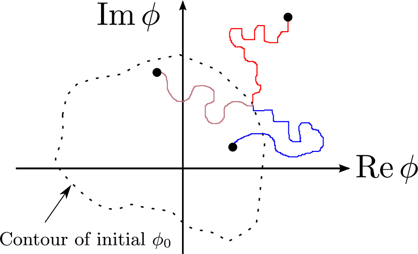
Figure 1: Sketch of stochastic realisations of the evolution of pseudo-population $\phi(t)$ in the complex plane according to Eq. (14), starting from a point $\phi_{0}$ on a contour that encircles the origin. An average over all end-points, three examples of which are shown as filled circles, corresponds to the quantity $\langle\phi\rangle_{\phi_{0}}$.

We could equally well employ the representation $\overline{A(N)}=\int f(\phi,t)\hat{A}(\phi)d^{2}\phi$ together with the associated 2-d integral versions of Eqs. (19) and (20) to obtain an analogous result $\overline{A(N)}=\int d^{2}\phi_{0}f(\phi_{0},0)\langle\hat{A}(\phi)\rangle_{\phi_{0}}$ which is particularly convenient for a initial Poisson distribution of population, such that $\overline{A(N)}=\langle\hat{A}(\phi)\rangle_{\lambda}$, where $\lambda$ is the initial mean.

II.4 Noise-averaged pseudo-population

We now establish the statistical properties of the stochastic variable $\phi(t)$. Our strategy will be to represent $\langle\phi\rangle_{\phi_{0}}$, the average of Eq. (15) over the noise for a given initial value $\phi_{0}$, as a (formal) series in positive powers of $\phi_{0}$, written

$$\!\!\langle\phi\rangle_{\phi_{0}} = \sum_{j=1}^{\infty}C_{j}(t)\phi_{0}^{j}=\phi_{0}\sum_{n=0}^{\infty}(-1)^{n}(\kappa\phi_{0})^{n}M_{n}(t),$$ (23)

with $C_{j}(t)=(-\kappa)^{j-1}M_{j-1}(t)$ and where

$$M_{j}(t)=\left\langle e^{\kappa t+i(2\kappa)^{1/2}W_{t}}\left(\int_{0}^{t}e^{\kappa s+i(2\kappa)^{1/2}W_{s}}ds\right)^{j}\right\rangle.$$ (24)

In Appendix B these coefficients are evaluated. We find that $m_{n}(\kappa t)=[(2\kappa)^{n}/n!]M_{n}(t)$ satisfy the recursion relation

$$m_{n}=\sum_{l=1}^{n}\frac{2^{l}(2n-l)!(-1)^{l+1}}{(2n)!l!}m_{n-l},$$ (25)

with

$$m_{0}(n)=1-\exp[-n(n+1)\kappa t],$$ (26)

and thus all the $m_{n}$ may be generated, for example $m_{1}=1-\exp(-2\kappa t)$ and $m_{2}=\frac{1}{6}\left(2-3e^{-2\kappa t}+e^{-6\kappa t}\right)$, and hence all the $C_{j}$ in Eq. (23). In Appendix C we explore how these coefficients, and the formal power series, allow us to determine the mean and variance of the particle population as a function of time and initial condition, recovering known results.

II.5 Averaged pseudo-population as $t\to\infty$

It will prove to be useful for comparisons with numerical work to determine the value of $\langle\phi\rangle_{\phi_{0}}$ as $t\to\infty$. Using Ito’s lemma we have

$$d\phi^{n}=n\phi^{n-1}d\phi+\frac{1}{2}(-2\kappa\phi^{2})n(n-1)\phi^{n-2}dt,$$ (27)

and we insert Eq. (14) and average such that

$$d\langle\phi^{n}\rangle=-\kappa n\langle\phi^{n+1}\rangle dt-\kappa n(n-1)\langle\phi^{n}\rangle dt.$$ (28)

Assuming that as $t\rightarrow\infty$ all the $\langle\phi^{n}\rangle$ become time independent, we deduce that $\langle\phi^{n+1}\rangle=-(n-1)\langle\phi^{n}\rangle$ in this limit, in which case all moments for $n\geq 2$ tend to zero, for all initial conditions.

Next, we note that

$$d(e^{-\phi})=-e^{-\phi}d\phi-\kappa\phi^{2}e^{-\phi}dt=-i(2\kappa)\phi e^{-\phi}dW_{t},$$ (29)

using Eq. (14), such that $d\langle\exp(-\phi)\rangle=0$, and imposing the initial condition we obtain $\langle\exp(-\phi)\rangle_{\phi_{0}}=\exp(-\phi_{0})$ for all $t$. Since

$$\langle e^{-\phi}\rangle_{\phi_{0}}=\sum_{n=0}^{\infty}\frac{(-1)^{n}}{n!}\langle\phi^{n}\rangle_{\phi_{0}},$$ (30)

we find that $\langle e^{-\phi}\rangle_{\phi_{0}}\to 1-\langle\phi\rangle_{\phi_{0}}$ as $t\to\infty$, due to the vanishing of moments with $n\geq 2$, and we conclude that the stochastic dynamics of $\phi(t)$ give rise to the asymptotic behaviour

$$\langle\phi\rangle_{\phi_{0}}\to 1-\exp(-\phi_{0})$$ (31)

in the late time limit. We shall use this result to check the outcomes of numerical calculations in Section III. The result makes sense because the mean population arising from a Poisson distribution with mean $\lambda$ at $t=0$ is equal to $\langle\phi\rangle_{\phi_{0}=\lambda}$. Intuitively, all initial situations sampled from such a distribution lead to a final population of unity as $t\to\infty$ except for the case of an initial population of zero, the probability of which is $\exp(-\lambda)$. An initial situation that leads to a final population of unity is therefore selected with probability $1-\exp(-\lambda)$. The mean population as $t\to\infty$ is $\overline{N}=0\times\exp(-\lambda)+1\times(1-\exp(-\lambda))=1-\exp(-\lambda)$.

We can confirm this result by considering kinetics starting from a definite initial population $N_{0}$. From Eq. (62) we write

$$\overline{N}\to\oint_{C}d\phi_{0}\frac{N_{0}!}{2\pi i}\phi_{0}^{-N_{0}-1}\exp(\phi_{0})\left(1-\exp(-\phi_{0})\right)$$ (32)

$$=\oint_{C}d\phi_{0}\frac{N_{0}!}{2\pi i}\phi_{0}^{-N_{0}-1}\sum_{n=1}^{\infty}\frac{1}{n!}\phi_{0}^{n}$$

$$=\sum_{n=1}^{\infty}\delta_{N_{0}n}=1-\delta_{N_{0}0},$$

demonstrating that the asymptotic mean population is unity, unless $N_{0}=0$ in which case it is zero.

II.6 Source enhanced coagulation

We can also determine the asymptotic behaviour of a system of coagulating species in which there is an injection rate $j$, to be used as a check in later numerical calculations. The underlying master equation is

$$\frac{dP(N,t)}{dt}=jP(N-1,t)-jP(N,t)+$$ (33)

$$\kappa(N+1)NP(N+1,t)-\kappa N(N-1)P(N,t),$$

with the first term deleted for the case $N=0$. The evolution of the corresponding pseudo-population is given by

$$d\phi=jdt-\kappa\phi^{2}dt+i(2\kappa)^{1/2}\phi dW_{t}.$$ (34)

This time we find that

$$d(e^{-\phi})=-e^{-\phi}d\phi-\kappa\phi^{2}e^{-\phi}dt$$ (35)

$$=-je^{-\phi}dt-i(2\kappa)^{1/2}\phi e^{-\phi}dW_{t},$$

so that $d\langle e^{-\phi}\rangle=-j\langle e^{-\phi}\rangle dt$ and $\langle e^{-\phi}\rangle\propto e^{-jt}$, with the proportionality factor depending on the initial condition. We also have

$$d\langle\phi^{n}\rangle=n\langle\phi^{n-1}\left(j-\kappa\phi^{2}\right)\rangle dt-\kappa n(n-1)\langle\phi^{n}\rangle dt,$$ (36)

which in a stationary state implies, for $n\geq 1$, that

$$\langle\phi^{n+1}\rangle_{{\rm st}}=\frac{j}{\kappa}\langle\phi^{n-1}\rangle_{{\rm st}}-(n-1)\langle\phi^{n}\rangle_{{\rm st}}.$$ (37)

This is reminiscent of a recurrence relation M. Abramowitz and I. A. Stegun (1972) for modified Bessel functions, $I_{n-1}(x)-I_{n+1}(x)=(2n/x)I_{n}(x)$, which suggests that $\langle\phi^{n}\rangle_{{\rm st}}\propto(j/\kappa)^{n/2}I_{n-1}(2(j/\kappa)^{1/2})$ for $n\geq 0$. Since $\langle\phi^{2}\rangle_{{\rm st}}=j/\kappa$ , the proportionality factor is $\left[I_{1}(2(j/\kappa)^{1/2})\right]^{-1}$. Notice that we do not label these stationary averages according to $\phi_{0}$ since memory of the initial condition is lost for this case. In the stationary state of a source enhanced coagulating system we therefore expect the mean population to be

$$\overline{N}_{{\rm st}}=\langle\phi\rangle_{{\rm st}}=\left(\frac{j}{\kappa}\right)^{1/2}\frac{I_{0}\left(2(j/\kappa)^{1/2}\right)}{I_{1}\left(2(j/\kappa)^{1/2}\right)},$$ (38)

which is similar to analysis performed elsewhere Gardiner (2009); Green et al. (2001); Lushnikov et al. (2003). The limit of this result as $j\to 0$ does not correspond to Eq. (31) since dependence on the initial condition reappears when $j=0$.

II.7 Remarks

We conclude our analytical consideration by noting that the coagulation problem can be studied in a variety of ways, and that introducing complex, stochastically evolving pseudo-populations, averaged over the noise and over a complex contour of initial values (or over the entire plane), might seem very elaborate compared with the direct analytic solution to the master equations, for example. Our purpose, however, is to establish explicitly that the approach works for a simple case. Our attention now turns to the numerical solution of the stochastic dynamics and averaging procedure to determine whether this can be performed efficiently for the model. Establishing this would suggest that a wider set of stochastic problems based on master equations might be amenable to solution using these techniques.

III Numerical approach

III.1 Stochastic numerics

An analytical solution to the SDEs corresponding to more complicated coagulation schemes, for example those modelled in the mean field approximation using rate equations such as (6), is unlikely to be available. In these cases our approach is implemented through a numerical solution of the SDEs for the relevant pseudo-populations $\phi_{i}(t)$, followed by averaging over the noise and a suitable weighting of the results over the initial values $\phi_{i0}$. We test the feasibility of this strategy for the simple $A+A\to A$ model.

We solve the SDE (14) numerically using a C++ code. In Figure 2, we plot $\mathrm{Re}\langle\phi\rangle_{\phi_{0}}$ against $t$ for $\phi_{0}=1$, 2 and 3, averaging $\phi$ over $10^{3}$ trajectories driven by independent realisations of the Wiener process using $10^{5}$ timesteps of length $5\times 10^{-5}$, and with $\kappa=1$. Also shown are analytical results based on the formal series developed in Section II.4 and Appendix B, truncated at the 12th power of $\phi_{0}$. This representation of the analytical solution appears to be accurate for the chosen values of $\phi_{0}$. Asymptotically, the series approximates well to values $1-\exp(-\phi_{0})$, in agreement with the analysis in Section II.5. For small $t$ the outcomes resemble the mean field result Eq. (4), as we suggest they should in Appendix D.

However, the numerical results do not appear to be very satisfactory. Firstly, the averages are noisy, suggesting that $10^{3}$ realisations are too few in number to obtain statistical accuracy, though this can of course be increased. Secondly, they do not seem to possess the correct limits at large times: they all seem to tend towards unity. Thirdly, they often exhibit sharp peaks, which are sometimes large enough to cause the numerical simulation to fail, as is seen in the case for $\phi_{0}=3$, where a negative spike at $t\approx 2.85$ causes the computation to crash. These instabilities, even if not terminal, have a disproportionate effect on the statistics when the number of realisations is limited. Such instabilities have been encountered before in simulations Drummond (2004); Gardiner (2009), and in the next section we examine their origin and consider how they can be avoided.

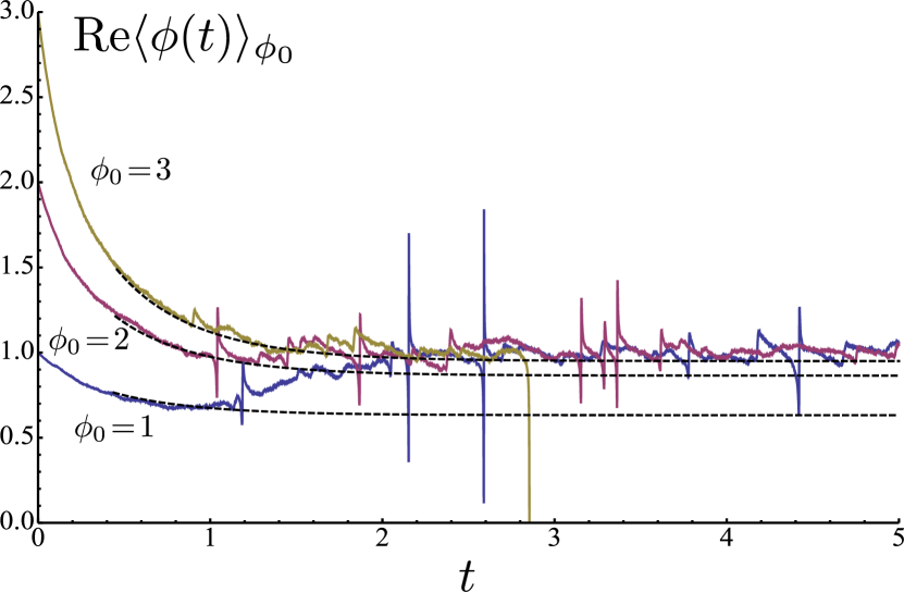
Figure 2: Numerical solutions to SDE (14), averaged over $10^{3}$ realisations of the noise with a timestep of $5\times 10^{-5}$ and $\kappa=1$, and with initial values $\phi_{0}=1$, 2 and 3, compared with series representations of $\langle\phi\rangle_{\phi_{0}}$ (dashed lines) including terms up to 12th order in $\phi_{0}$, as derived in Section II.4.

III.2 Elimination of instabilities

The origin of the large fluctuations in $\phi(t)$ can be understood by considering the deterministic contribution to its evolution in the complex plane according to Eq. (14). This is shown schematically by block arrows in Figure 3, representing the magnitude and orientation of the complex quantity $-\phi^{2}$. Were it not for stochastic noise, a trajectory that started with a positive value of Re$\phi$ would remain in the right hand side of the complex plane and indeed would drift asymptotically towards the origin. The picture is quite different for a negative initial value of Re$\phi$: there is a component of drift away from the origin, though in most cases the path ultimately moves around into the right hand side of the plane and from there to the origin. The exception is for trajectories starting on the negative real axis, which asymptotically move towards $-\infty$. This pattern of drift has the potential for instability.

Of course the evolution of $\phi$ is also driven by noise, and an example trajectory is shown in Figure 3. For much of the time $\phi$ evolves in a rather well-behaved fashion over the complex plane, forming a crescent shaped trace. The noise maintains the trajectory away from the deterministic attractor at the origin. However, noise is also the undoing of this stability: if the trajectory wanders onto the left hand side of the plane driven by the stochastic term in Eq. (14), then a tendency to drift towards $\phi=-\infty$ can set in. This is also shown in Figure 3: at some point a fluctuation causes $\phi(t)$ to move towards the left, away from the crescent pattern. In this example, quite a significant excursion towards negative real values occurs before noise deflects the trajectory sufficiently away from the real axis, allowing the underlying drift to take $\phi(t)$ in an anticlockwise fashion back towards the right hand side of the plane. Once there, the $\phi(t)$ settles again into the crescent pattern. The intervals spent within the crescent correspond to those periods in Figure 2 where fluctuations are small, whilst excursions into the left hand plane seem to be responsible for the spikes Deloubrière et al. (2002).

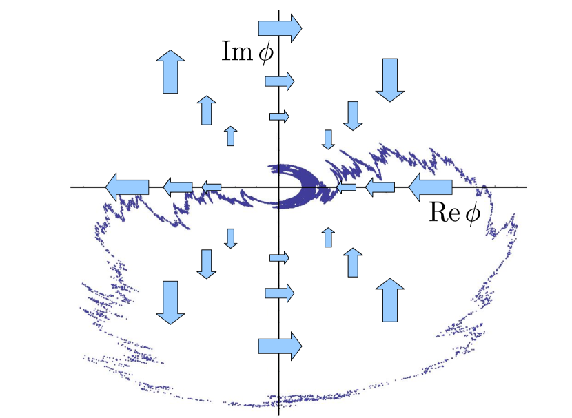
Figure 3: The block arrows indicate the magnitude and direction of drift of $\phi(t)$ across the complex plane brought about by the deterministic term $-\kappa\phi^{2}dt$ in the SDE (14). The effect of this pattern is seen in an example realisation of the evolution. An excursion towards negative Re$(\phi)$ from the quasistable crescent shaped region near the origin, followed by a return path taken in an anticlockwise direction, is responsible for a spike in the average of $\phi$ shown in Figure 2.

These instabilities are not desirable and action should be taken to eliminate them. They are less common if the timestep in the numerical simulation is reduced, since this lowers the likelihood of a noise-driven jump into the left hand side of the complex plane, but this increases the computational expense of the approach. We therefore need a mathematical scheme that can suppress the dangerous drift pattern in the stochastic dynamics while retaining the statistical properties of solutions to the SDE.

Drummond Drummond (2004) proposed a scheme for the elimination of such instabilities, taking the form of a modification to the fundamental Poisson representation through the introduction of a weighting parameter $\Omega(t)$, chosen to evolve according to

$$d\Omega=\Omega gdW_{t},$$ (39)

with initial condition $\Omega(0)=1$, and where $g$ is an arbitrary function. A new variable $\phi^{\prime}$ is introduced, subject to the same initial condition imposed on $\phi$, but evolving according to

$$d\phi^{\prime}=-\kappa\phi^{\prime 2}dt+i(2\kappa)^{1/2}\phi^{\prime}\left(dW_{t}-gdt\right),$$ (40)

and Drummond showed that the $\Omega$-weighted average of $\phi^{\prime}$ over the noise is the same as the corresponding average of $\phi$:

$$\langle\phi\rangle=\langle\Omega\phi^{\prime}\rangle.$$ (41)

However, since $\phi^{\prime}$ and $\phi$ evolve according to different SDEs, they need not suffer from the same instabilities.

Drummond termed this the ‘gauging away’ of the instabilities of the original SDE, the terminology suggested by recognising that Eq. (41) possesses an invariance with respect to different choices of $g$. The evolution of $\phi^{\prime}$ and $\Omega$ is affected by the form of $g,$ but not $\langle\phi\rangle$. In other areas of theoretical physics, especially in electromagnetism and quantum field theories, a gauge transformation is precisely a recasting of a theoretical problem that has no effect on the eventual physical predictions, and hence the terminology is appropriate. The transformation can be useful mathematically but is arbitrary as far as the physics is concerned.

The approach is in fact equivalent to a transformation of the probability measure in stochastic calculus, and can be perhaps be most easily understood as an application of the Cameron-Martin-Girsanov formula Cameron and Martin (1944, 1945); Girsanov (1960) in stochastic calculus, as we describe in more detail in Appendix E.

We explore one of Drummond’s gauge functions $g(\phi^{\prime})$ that has the capacity to tame the instability in the coagulation problem. Consider the choice

$$g=i\left(\kappa/2\right)^{1/2}\left(\phi^{\prime}-|\phi^{\prime}|\right),$$ (42)

which leads to the SDEs

$$d\phi^{\prime}=-\kappa\phi^{\prime}|\phi^{\prime}|dt+i(2\kappa)^{1/2}\phi^{\prime}dW_{t},$$ (43)

and

$$d\Omega=i\left(\kappa/2\right)^{1/2}\left(\phi^{\prime}-|\phi^{\prime}|\right)\Omega dW_{t}.$$ (44)

The crucial difference between Eqs. (43) and (14) is that the drift term in the SDE for $\phi^{\prime}$ is always directed towards the origin. It lacks the ability to produce an excursion towards $\phi^{\prime}=-\infty$. Meanwhile, $\Omega(t)$ evolves diffusively in the complex plane, with no drift and hence $d\langle\Omega\rangle=0$. As long as $\phi^{\prime}$ is real, the increment $d\Omega$ vanishes, and because of this feature, Drummond called this choice of $g$ a minimal gauge function, and regarded it as a natural choice for cases where $\phi^{\prime}$ is expected to take real values for most of its history.

We have studied this reformulation of the coagulation problem and confirmed numerically that $\phi^{\prime}(t)$ does not suffer from instabilities of the kind experienced by $\phi(t)$, and that the $\Omega$-weighted average of $\phi^{\prime}$ appears to agree with various analytic results expected for $\langle\phi\rangle_{\phi_{0}}$, as shown in Figure 4. Nevertheless, we notice that the statistical uncertainty in the average of $\Omega(t)$ grows as time progresses, and this introduces a decline in accuracy, for a given number of realisations. We next address the reasons for this.

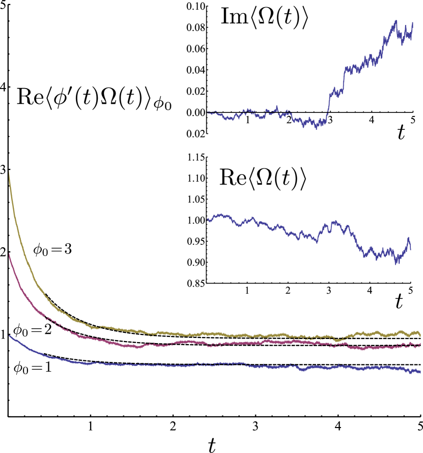
Figure 4: Evolution of Re$\langle\phi^{\prime}\Omega\rangle_{\phi_{0}}$ according to Eqs. (43) and (44), with $\kappa=1$ and $\phi_{0}=1$, 2 and 3, for the same timestep and number of realisations as in Figure 2. The expected analytic behaviour is indicated, and in comparison with Figure 2 the noise in the numerical results is much reduced, which is a consequence of the gauging procedure. The evolution of the real and imaginary parts of $\langle\Omega\rangle$ for the case with $\phi_{0}=2$ is shown in the inset, to illustrate the deviation from the expected values of unity and zero, respectively, as $t$ increases: this is caused by sampling errors.

III.3 Asymptotic behaviour of $\Omega$

The diffusive behaviour of the weight function $\Omega$ can be best demonstrated by considering the evolution of the mean of $|\Omega|^{2}$. We have $d\Omega=g\Omega dW_{t}$ and hence $d\Omega^{*}=g^{*}\Omega^{*}dW_{t}$ such that, using Ito’s lemma

$$d|\Omega|^{2}=\Omega d\Omega^{*}+\Omega^{*}d\Omega+g\Omega g^{*}\Omega^{*}dt$$ (45)

$$=\Omega g^{*}\Omega^{*}dW_{t}+\Omega^{*}g\Omega dW_{t}+|g|^{2}|\Omega|^{2}dt,$$

and so

$$d\langle|\Omega|^{2}\rangle=\langle|g|^{2}|\Omega|^{2}\rangle dt,$$ (46)

which indicates that the mean square modulus of $\Omega$ increases monotonically, whatever choice of function $g$ is made. The mean of $\Omega$ is unity for all $t$, but its increasing mean square modulus suggests that the distribution of $\Omega$ broadens as $t$ increases. As a consequence, the accurate extraction of the statistical properties of the dynamics will require more realisations for larger $t$. This is the price to pay, it seems, for the taming of the instabilities in the original SDE.

III.4 Optimised gauge

Nevertheless, the choice available to us in the gauging procedure, or equivalently the freedom to shift the probability measure according to the Cameron-Martin-Girsanov formula (see Appendix E), allows us to optimise the quality of the numerical estimates of $\langle\phi\rangle$. Consider a new gauge function containing the real variable $R$:

$$g=i\left(\kappa/2\right)^{1/2}\left(\phi^{\prime}-|\phi^{\prime}|-R\right),$$ (47)

which differs from Eq. (42) by an imaginary constant. It leads to the SDEs

$$d\phi^{\prime}=-\kappa\phi^{\prime}\left(R+|\phi^{\prime}|\right)dt+i(2\kappa)^{1/2}\phi^{\prime}dW_{t},$$ (48)

and

$$d\Omega=i\left(\kappa/2\right)^{1/2}\left(\phi^{\prime}-|\phi^{\prime}|-R\right)\Omega dW_{t},$$ (49)

with the property $\langle\phi\rangle=\langle\Omega\phi^{\prime}\rangle$. Intuitively, a positive $R$ has the effect of strengthening the drift towards the origin in the SDE for $\phi^{\prime}$. It is revealing to study the evolution of the square modulus of $\phi^{\prime}$ under this gauge. We write

$$d(\phi^{\prime}\phi^{\prime*})=\phi^{\prime}d\phi^{\prime*}+\phi^{\prime*}d\phi^{\prime}+i(2\kappa)^{1/2}\phi^{\prime}\left[-i(2\kappa)^{1/2}\phi^{\prime*}\right]dt$$

$$=-\kappa|\phi^{\prime}|^{2}\left(R+|\phi^{\prime}|\right)dt-i(2\kappa)^{1/2}|\phi^{\prime}|^{2}dW_{t}$$

$$\quad-\kappa|\phi^{\prime}|^{2}\left(R+|\phi^{\prime}|\right)dt+i(2\kappa)^{1/2}|\phi^{\prime}|^{2}dW_{t}+2\kappa|\phi^{\prime}|^{2}dt,$$ (50)

so

$$d|\phi^{\prime}|^{2}=2\kappa(1-R)|\phi^{\prime}|^{2}-2\kappa|\phi^{\prime}|^{3},$$ (51)

and thus $|\phi^{\prime}|$ evolves deterministically towards an asymptotic value of $(1-R)$, if $R\leq 1$, or zero if $R>1$.

It is also revealing to consider the SDE for $\Omega\phi^{\prime}$ explicitly:

$$d(\Omega\phi^{\prime})=\phi^{\prime}d\Omega+\Omega d\phi^{\prime}$$

$$\quad+i\left(\kappa/2\right)^{1/2}\left(\phi^{\prime}-|\phi^{\prime}|-R\right)\Omega i(2\kappa)^{1/2}\phi^{\prime}dt$$

$$=\phi^{\prime}i\left(\kappa/2\right)^{1/2}\left(\phi^{\prime}-|\phi^{\prime}|-R\right)\Omega dW_{t}$$

$$\quad+\Omega\left(-\kappa\phi^{\prime}\left(R+|\phi^{\prime}|\right)dt+i(2\kappa)^{1/2}\phi^{\prime}dW_{t}\right)$$

$$\quad-\kappa\phi^{\prime}\Omega\left(\phi^{\prime}-|\phi^{\prime}|-R\right)dt$$

$$=-\kappa\Omega\phi^{\prime 2}dt+i\left(\kappa/2\right)^{1/2}\phi^{\prime}\left(\phi^{\prime}-|\phi^{\prime}|-R+2\right)\Omega dW_{t},$$ (52)

such that as $t\to\infty$ the stochastic term on the right hand side tends towards either $i\left(\kappa/2\right)^{1/2}\phi^{\prime}\left((1-R)\exp[i{\rm\,arg}(\phi^{\prime})]+1\right)\Omega dW_{t}$ if $R\leq 1$, or $i\left(\kappa/2\right)^{1/2}\phi^{\prime}\left(2-R\right)\Omega dW_{t}$ if $R>1$. Furthermore, the evolution of the average square modulus of $\Omega$ is described by

$$\begin{aligned} &d\langle|\Omega|^{2}\rangle=\frac{\kappa}{2}\langle|\phi^{\prime}-|\phi^{\prime}|-R|^{2}|\Omega|^{2}\rangle dt\end{aligned},$$ (53)

which tends to $\frac{1}{2}\kappa\langle|(1-R)\exp[i\,{\rm arg}(\phi^{\prime})]-1|^{2}|\Omega|^{2}\rangle dt$ if $R\leq 1$, or $\frac{1}{2}\kappa R{}^{2}\langle|\Omega|^{2}\rangle dt$ if $R>1$.

This analysis indicates that there are advantages in making specific choices of $R$. If we choose $R=2$, Eq. (52) shows that we can eliminate the noise term controlling the asymptotic time evolution of $\Omega\phi^{\prime}$. On the other hand, it is the diffusive behaviour of $\Omega$ that characterises the asymptotic statistics of other quantities. The strength of the diffusion depends on the quantity $(1-R)^{2}-2(1-R)\cos{\rm arg}(\phi^{\prime})+1$ for $R\leq 1$, and $R^{2}$ for $R>1$. It is clear that the asymptotic rate of diffusive spread of $\Omega$ increases as $R$ becomes large, which is disadvantageous.

As a consequence, we have explored gauges specified by values of $R$ between zero and two. As $R$ increases, the diffusive behaviour of $\Omega$ becomes more marked while the noise in the evolution of $\Omega\phi^{\prime}$ reduces. We find that the choice $R=1$ strikes a balance by suppressing noise in the evolution of ${\rm Re}\langle\phi\rangle_{\phi_{0}}={\rm Re}\langle\Omega\phi^{\prime}\rangle_{\phi_{0}}$, at the price of more significant statistical deviations of Re$\langle\Omega\rangle$ from the expected value of unity than in the case $R=0$. This is illustrated in Figure 5 which is to be compared with Figure 4. The shift in gauge seems to have transferred the statistical noise from $\langle\Omega\phi^{\prime}\rangle$ into $\langle\Omega\rangle$. We suggest that $R=1$ specifies an optimised gauge for this stochastic problem.

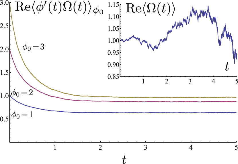
Figure 5: Evolution of Re$\langle\Omega\phi^{\prime}\rangle_{\phi_{0}}$ gauged according to the improved procedure described by Eqs. (48) and (49) with $R=1$, for initial conditions $\phi_{0}=1$, 2 and 3. This should be compared with the results from Eqs. (43) and (44) in Figure 4, obtained with the same timestep and number of realisations but using $R=0$. The evolution is less affected by statistical noise and corresponds very closely to the expected analytic behaviour. The evolution of $\Omega$ is more noisy, however, as indicated in the inset.

III.5 Further calculations

Using the gauge function (47) with $R=1$ we can study further aspects of the pseudo-population dynamics that were investigated analytically in Section II. For particle coagulation starting from a Poisson distribution with mean $\lambda$ the averages are simply given by quantities $\overline{A(N)}=\langle\hat{A}(\phi)\rangle_{\lambda}$. In Figure 6 we plot the evolution of a selection of state probabilities $P(N,t)$ for $\lambda=5$, derived from Eq. (18), together with the solutions to Eq. (1) for a similar case with the initial Poisson distribution truncated at $N=12$ for convenience. The timestep and number of realisations are the same as in earlier cases. The correspondence is very good, and the noise does not significantly distort the results over the time scale for the completion of the coagulation.

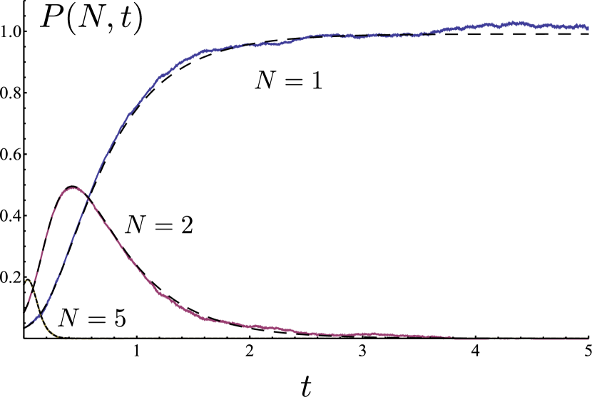
Figure 6: Probabilities of the occurrence of five, two and one particle as coagulation progresses for $\kappa=1$, starting from a Poisson distribution with mean $\lambda=5$ at $t=0$, comparing numerical evaluations of Eq. (18), gauged through Eq. (47) with $R=1$ (solid lines) with solutions to the master equations (1) (dashed lines).

Finally, we examine source enhanced coagulation modelled by Eq. (34), with the use of the optimised gauge. The quantities $\langle\phi\rangle=\langle\Omega\phi^{\prime}\rangle$ and $\langle\phi^{2}\rangle=\langle\Omega\phi^{\prime 2}\rangle$ are plotted for $j=\kappa=1$ in Figure 7 to show they compare well with the analytical results for late times obtained in Section II.6. The initial condition is a Poisson distribution with $\lambda=2$. However, to indicate that not all quantities are statistically well represented, we also show the average of $\exp(-\phi)$, which ought to equal $\exp(-2-jt$) for this case. Clearly more realisations would be needed to reproduce this behaviour accurately with this choice of gauge.

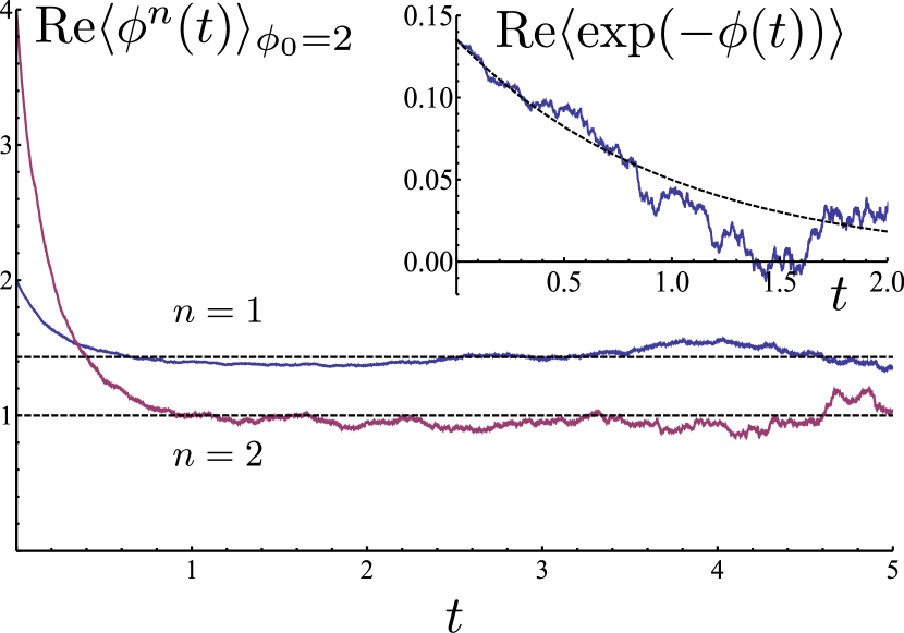
Figure 7: Main image: evolution of $\langle\phi\rangle_{\phi_{0}}$ and $\langle\phi^{2}\rangle_{\phi_{0}}$ (solid lines) according to the source enhanced coagulation kinetics embodied in Eq. (34), with $j=\kappa=1$, initial condition $\phi_{0}=\lambda=2$, and $10^{3}$ realisations with time step $5\times 10^{-5}$. At late times they correspond well to the stationary values $\langle\phi\rangle_{{\rm st}}=I_{0}(2)/I_{1}(2)\approx 1.43$ and $\langle\phi^{2}\rangle_{{\rm st}}=1$ (dashed lines) derived in Section II.6. Inset: a numerical calculation of the real part of $\langle\exp(-\phi)\rangle$ (solid line) is compared with the expected behaviour $\exp(-2-jt$) (dashed line), to illustrate that not every variable has acceptable statistics for this number of realisations of the stochastic evolution.

IV Discussion

We have outlined in this paper how to solve a simple coagulation problem using some rather elaborate analytical and numerical methods, retrieving results that were previously either known, or computable from the master equations. The effort has not been misdirected, however, since our aim has been to establish that the approach can be implemented successfully for a well characterised example problem. The greater part of our interest lies in more complicated cases of coagulation such as those with multiple species that agglomerate at a variety of rates. In such systems we expect to find behaviour that arises due to statistical fluctuations around low mean populations that cannot be captured in the usual mean field formulation. We plan to address such cases in further work.

Specifically, we employ a Poisson representation Gardiner and Chaturvedi (1977); Gardiner (2009) of the probability $P(N,t)$ that there should be $N$ particles present at time $t$ in the simple case of $A+A\to A$ kinetics. The Poisson representation is a superposition of Poisson distributions with complex means. The description can be cast as a problem in the stochastic dynamics of a complex pseudo-population, the average of which over the noise and the initial condition is related to the average of the physical particle population. Analytical work gives a series expansion of this average in powers of the initial value of the pseudo-population, and this can be employed to recover known results Green et al. (2001); Deloubrière et al. (2002); Lushnikov et al. (2003); Täuber et al. (2005); Barzykin and Tachiya (2005); Hochberg et al. (2006). The development of the series involves the evaluation of multiple integrals of functions of the Wiener process. We have also identified some exact results valid in the limit $t\to\infty$, and in Appendix D give an approximate result for small $\kappa t$ that resembles a mean field solution to the kinetics. We have discussed the evaluation of averages of general functions of the population, such as higher moments. We have also studied the stationary state of a coagulating system enhanced by a constant injection of new particles.

Analytical work can only be performed in certain circumstances, and more generally a numerical solution of the stochastic differential equations (SDEs) is necessary, followed by averaging over noise and initial condition. Unfortunately, numerical instabilities make this problematic, as has been noted previously Deloubrière et al. (2002); Drummond (2004); Gardiner (2009). However, we follow Drummond Drummond (2004) in identifying an SDE for a pseudo-population that is free of instabilities, to be used together with a weighting procedure that reproduces the statistics of the desired system. In Appendix E we have shown that this ‘gauging’ scheme is equivalent to an adaptive shift in the probability measure for the stochastic variable in the SDE, and that the weighting procedure is an application of the Cameron-Martin-Girsanov formula. This interpretation arguably makes the gauging procedure more intuitive.

We have identified a choice of gauge, and associated transformation of the problem, that provides statistical information in a rather optimised fashion. With this approach, the growth with time in the statistical uncertainty that is inherent with gauging can be adequately controlled, such that we need to generate relatively few realisations of the evolution, requiring rather little computational effort. A number of the analytically derived results have been reproduced using this numerical approach.

Of course Monte Carlo (MC) simulation of coagulation events taking place in an evolving population of particles would be an obvious alternative numerical method for studying this system. It is readily implemented, for example using the Gillespie algorithm Gillespie (1977), and has the capacity to include population fluctuation effects. It is an approach that is probably easier to grasp than the methods we have outlined, and more computationally efficient for the problem under consideration here. Nevertheless, we believe that pseudo-population methods will prove to be more efficient than MC in coagulation problems involving multiple species.

This point can be made by counting the number of master equations that would effectively be solved by an MC procedure. If we wish to study the evolution of clusters of monomers that have size dependent agglomeration properties, then each size must be treated as a distinct species. If we consider clusters ranging in size from 1 to $N_{{\rm max}}$ monomers, then master equations describing the evolution of probabilities $P(N_{1},N_{2},\cdots,N_{N_{{\rm max}}},t)$ must be solved, where $N_{i}$ denotes the population of clusters of size $i$. If each population can vary between 0 and $n_{i}^{{\rm max}}$, then the number of elementary population distributions that must be considered is of order $\prod_{i=1}^{N_{{\rm max}}}\left(n_{i}^{{\rm max}}+1\right)$. It is reasonable to say that this number can become rather large and will grow faster than $N_{{\rm max}}$. The solution to such a large number of coupled ordinary differential equations, or the equivalent MC simulation, would be daunting.

On the other hand, the stochastic approach requires the solution to just $N_{{\rm max}}$ SDEs for pseudo-populations $\phi_{i}(t)$; these are analogues of the mean populations of clusters of size $i$. The SDEs would bear some resemblance to the Smoluchowski coagulation equations for mean populations in the mean field, fluctuation-free limit, given in Eq. (6). Analytic solution to these equations might be unavailable, but numerical solution would not be difficult, especially if we have techniques such as gauging at our disposal to avoid some of the pitfalls we have identified. The drawback is that averaging of the SDEs over a variety of noise histories and perhaps initial conditions is necessary. Nevertheless, the task is linear in $N_{{\rm max}}$ and must eventually become more efficient than direct solution to the master equations as $N_{{\rm max}}$ increases.

It is only when the mean of a population becomes small that deviations from mean field behaviour emerge, and so a hybrid approach might be possible whereby mean field rate equations are used to model the early stages of coagulation, going over to pseudo-population rate equations when the mean population becomes small. This is possible since the mean field rate equations closely resemble the evolution equations of the pseudo-populations, which is an important conceptual and mathematical point of correspondence. Specifically, we could integrate the equations for the $\phi_{i}(t)$ with the neglect of the noise when the modulus of $\phi_{i}(t)$ is large, such that they remain real, and introduce noise, and average over it, only when the modulus becomes small.

In conclusion, we have made conceptual and numerical developments of a method for kinetic modelling that was introduced some time ago Gardiner and Chaturvedi (1977) but that appears not to have been fully exploited. We believe that in spite of some complexity in the formulation, the approach possesses considerable intuitive value, and that it has the capability to treat systems with interesting statistical properties for which alternative methods are inappropriate or expensive. We intend to explore these possibilities in further studies.

Appendix A Stochastic evolution of a complex pseudo-population

We solve Eq. (14) to justify the expression for $\phi(t)$ given in Eq. (15). Consider $G(\phi,x)=\phi^{-1}\exp(x)$ with stochastic variables evolving according to $d\phi=adt+bdW_{t}$ and $dx=pdt+qdW_{t}$. By Ito’s lemma we have

$$dG=\frac{\partial G}{\partial\phi}d\phi+\frac{\partial G}{\partial x}dx+\frac{1}{2}b^{2}\frac{\partial^{2}G}{\partial\phi^{2}}dt+bq\frac{\partial^{2}G}{\partial\phi\partial x}dt+\frac{1}{2}q^{2}\frac{\partial^{2}G}{\partial x^{2}}dt,$$ (54)

so

$$dG=-\frac{1}{\phi}Gd\phi+Gdx+\frac{b^{2}}{\phi^{2}}Gdt-\frac{bq}{\phi}Gdt+\frac{q^{2}}{2}Gdt$$ (55)

$$=\left(-\frac{a}{\phi}+p+\frac{b^{2}}{\phi^{2}}-\frac{bq}{\phi}+\frac{q^{2}}{2}\right)Gdt+\left(-\frac{b}{\phi}+q\right)GdW_{t}.$$

In order to eliminate the noise term we choose $b=q\phi$, so that $dG=\left(-\phi^{-1}a+p+q^{2}/2\right)Gdt$. We set $q=i(2\kappa)^{1/2}$ and $p=\kappa$, in which case the SDE for $x$ integrates to give $x(t)=\kappa t+i(2\kappa)^{1/2}W_{t}$, having chosen initial condition $x(0)=0$. Furthermore, if $a=-\kappa\phi^{2}$ then

$$d\phi=-\kappa\phi^{2}dt+i(2\kappa)^{1/2}\phi dW_{t},$$ (56)

as desired, and $dG=\kappa\phi Gdt=\kappa e^{x}dt=\kappa\exp[\kappa t+i(2\kappa)^{1/2}W_{t}]dt$ which integrates to

$$G(t)=G(0)+\kappa\int_{0}^{t}\exp\left(\kappa s+i(2\kappa)^{1/2}W_{s}\right)ds.$$ (57)

Since $G(t)=\phi^{-1}\exp\left(\kappa t+i(2\kappa)^{1/2}W_{t}\right)$ and $G(0)=\phi_{0}^{-1}$, we then recover Eq. (15).

Appendix B Formal power series form of noise averaged pseudo-population

We provide the details of the derivation of the formal power series representation of $\langle\phi(t)\rangle_{\phi_{0}}$ starting from Eq. (15). The first order term, proportional to $\phi_{0}$, is straightforward: we write

$$\langle\phi\rangle_{\phi_{0}}\approx\int dW_{t}\,\phi_{0}\,\mathrm{exp}(\kappa t+i(2\kappa)^{\frac{1}{2}}W{}_{t}),$$ (58)

and use the stochastic integral identity $\int dW_{t}\exp(icW_{t})=\langle\exp(icW_{t})\rangle=\exp(-c^{2}t/2)$ such that

$$\langle\phi\rangle_{\phi_{0}}=\phi_{0}+O(\phi_{0}^{2}),$$ (59)

but higher order terms in the formal series

$$\langle\phi\rangle_{\phi_{0}} = \sum_{j=1}^{\infty}C_{j}(t)\phi_{0}^{j}=\phi_{0}\sum_{n=0}^{\infty}(-1)^{n}(\kappa\phi_{0})^{n}M_{n}(t)$$ (60)

with $C_{j}(t)=(-\kappa)^{j-1}M_{j-1}(t)$ and

$$M_{j}(t)=\left\langle e^{\kappa t+i(2\kappa)^{1/2}W_{t}}\left(\int_{0}^{t}e^{\kappa s+i(2\kappa)^{1/2}W_{s}}ds\right)^{j}\right\rangle.$$ (61)

require more work.

We focus our attention on the evolution of the mean particle population $\overline{N}$ for cases where $N_{0}$ particles are present at $t=0$. We use $P(N,0)=\delta_{NN_{0}}$ with Eqs. (22) and (10) to obtain

$$\overline{N}=\langle\phi\rangle=\oint_{C}d\phi_{0}\frac{N_{0}!}{2\pi i}\phi_{0}^{-N_{0}-1}\exp(\phi_{0})\langle\phi\rangle_{\phi_{0}},$$ (62)

and by inserting Eq. (60) and expanding the integrand we find that

$$\overline{N}=\sum_{j=1}^{N_{0}}C_{j}(t)\frac{N_{0}!}{(N_{0}-j)!}.$$ (63)

Notice that the number of coefficients $C_{j}$ required to evaluate $\overline{N}$ is finite even though the series for $\langle\phi\rangle_{\phi_{0}}$ is infinite.

We have already established that $C_{1}(t)=1$ in Eq. (59). In order to evaluate $C_{2}(t)$ we need to consider

$$I(t,s)=\left\langle\exp\left(i(2\kappa)^{1/2}\left(W_{t}+W_{s}\right)\right)\right\rangle,$$ (64)

which in more explicit form reads

$$I(t,s)=\int_{-\infty}^{\infty}dW_{t}dW_{s}\exp\left(i(2\kappa)^{1/2}\left(W_{t}+W_{s}\right)\right)$$

$$\times\frac{1}{(2\pi(t-s))^{1/2}}\exp\left(-\frac{(W_{t}-W_{s})^{2}}{2(t-s)}\right)$$ (65)

$$\times\frac{1}{(2\pi s)^{1/2}}\exp\left(-\frac{W_{s}^{2}}{2s}\right),$$

in which the weighting is a product of the gaussian probabilities for generating a value $W_{s}$ of the Wiener process at time $s$, and a value $W_{t}$ at the later time $t$ given the earlier value. Writing $W_{t}+W_{s}=W_{t}^{\prime}+2W_{s}$ where $W_{t}^{\prime}=W_{t}-W_{s}$ this factorises as follows:

$$I(t,s) = \int dW_{t}^{\prime}\exp\left(i(2\kappa)^{1/2}W_{t}^{\prime}\right)$$ (66)

$$\times \frac{1}{(2\pi(t-s))^{1/2}}\exp\left(-\frac{W_{t}^{\prime 2}}{2(t-s)}\right)$$

$$\times \int dW_{s}\exp(2i(2\kappa)^{1/2}W_{s})\frac{1}{(2\pi s)^{1/2}}\exp\left(-\frac{W_{s}^{2}}{2s}\right)$$

$$= \langle\exp(i(2\kappa)^{1/2}W_{t-s})\rangle\langle\exp(2i(2\kappa)^{1/2}W_{s})\rangle$$

$$= e^{-\kappa(t-s)}e^{-4\kappa s}=e^{-\kappa(t+3s)},$$

using $\langle\exp(icW_{t})\rangle=\exp(-c^{2}t/2)$, and hence $C_{2}(t)=-\kappa M_{1}(t)$ with

$$M_{1}(t)=e^{\kappa t}\int_{0}^{t}ds\,e^{\kappa s}\left\langle\exp\left(i(2\kappa)^{1/2}\left(W_{t}+W_{s}\right)\right)\right\rangle$$ (67)

$$=e^{\kappa t}\int_{0}^{t}ds\,e^{\kappa s}I(t,s)=\int_{0}^{t}ds\,e^{-2\kappa s}=\frac{1}{2\kappa}\left(1-e^{-2\kappa t}\right).$$

Consider next $C_{3}(t)=\kappa^{2}M_{2}(t)$. We need to evaluate

$$M_{2}=\int_{0}^{t}ds_{1}\int_{0}^{t}ds_{2}e^{\kappa(t+s_{1}+s_{2})}$$ (68)

$$\times\left\langle\exp\left[i(2\kappa)^{1/2}\left(W_{t}+W_{s_{1}}+W_{s_{2}}\right)\right]\right\rangle$$

$$=2\int_{0}^{t}ds_{1}\int_{0}^{s_{1}}ds_{2}e^{\kappa(t+s_{1}+s_{2})}$$

$$\times\left\langle\exp\left[i(2\kappa)^{1/2}\left(W_{t}-W_{s_{1}}+2(W_{s_{1}}-W_{s_{2}})+3W_{s_{2}}\right)\right]\right\rangle,$$

where an ordering $t\geq s_{1}\geq s_{2}\geq 0$ has been imposed by the choice of integration limits, the change in which is accounted for by inserting the prefactor of two. Once again this reduces to

$$M_{2}=2\int_{0}^{t}ds_{1}\int_{0}^{s_{1}}ds_{2}\exp(\kappa(t+s_{1}+s_{2}))$$ (69)

$$\times\exp\left(-\kappa(t-s_{1})\right)\exp\left(-4\kappa(s_{1}-s_{2})\right)\exp\left(-9\kappa s_{2}\right)$$

$$=2\int_{0}^{t}ds_{1}\int_{0}^{s_{1}}ds_{2}\exp(-2\kappa s_{1})\exp(-4\kappa s_{2}),$$

which becomes

$$M_{2} = \frac{1}{2\kappa}\int_{0}^{t}ds_{1}\exp(-2\kappa s_{1})\left(1-\exp(-4\kappa s_{1})\right)$$ (70)

$$= \frac{1}{2\kappa}\left[\frac{1}{2\kappa}\left(1-e^{-2\kappa t}\right)-\frac{1}{6\kappa}\left(1-e^{-6\kappa t}\right)\right].$$

Similarly, we can show that

$$M_{3}=6\int_{0}^{t}ds_{1}\int_{0}^{s_{1}}ds_{2}\int_{0}^{s_{2}}ds_{3}e^{-2\kappa s_{1}}e^{-4\kappa s_{2}}e^{-6\kappa s_{3}},$$ (71)

and the pattern that emerges is

$$M_{n}=n!\int_{0}^{t}ds_{1}\cdots\int_{0}^{s_{n-1}}ds_{n}e^{-2\kappa s_{1}}\cdots e^{-2n\kappa s_{n}}.$$ (72)

We notice that the $M_{n}$ are related to one another by repeated integration of the nested integrals. We define

$$m_{n}(\kappa t)=\frac{(2\kappa)^{n}}{n!}M_{n}(t)$$ (73)

$$=\int_{0}^{2\kappa t}ds_{1}\int_{0}^{s_{1}}ds_{2}\cdots\int_{0}^{s_{n-1}}ds_{n}e^{-s_{1}}e^{-2s_{2}}\cdots e^{-ns_{n}},$$

such that $m_{1}=1-\exp(-2\kappa t)$ and

$$m_{2}=\frac{1}{6}\left(2-3e^{-2\kappa t}+e^{-6\kappa t}\right)=\frac{1}{2}m_{1}-\frac{1}{6}\left(1-e^{-6\kappa t}\right).$$ (74)

Similarly we can show that

$$m_{3}=\frac{1}{3}m_{2}-\frac{1}{3}\frac{1}{5}m_{1}+\frac{1}{3}\frac{1}{5}\frac{1}{6}\left(1-e^{-12\kappa t}\right).$$ (75)

On the basis of an analysis of further cases, we conjecture a pattern

$$m_{n}=\frac{1}{n}m_{n-1}-\frac{m_{n-2}}{n[n+(n-1)]}$$ (76)

$$+\frac{m_{n-3}}{n[n+(n-1)][n+(n-1)+(n-2)]}$$

$$\cdots+(-1)^{n}\frac{m_{1}}{n\left[n+(n-1)\right]\cdots\left[n+(n-1)+\cdots+2\right]}$$

$$\!\!+(-1)^{n+1}\frac{1}{n\left[n+(n-1)\right]\cdots\left[n+(n-1)+\cdots+2\right]}$$

$$\!\!\times\!\int_{0}^{2\kappa t}\!\!\!ds_{1}\exp[-(n+[n-1]+\cdots+1)s_{1}].$$

This may be simplified since $n+(n-1)+\cdots+1=\frac{1}{2}n(n+1)$ is a triangular number, and

$$n+(n-1)+\cdots+(n-j+1)$$ (77)

$$=n+(n-1)+\cdots+1$$

$$-[(n-j)+(n-j-1)+\cdots+1]$$

$$=\frac{1}{2}n(n+1)-\frac{1}{2}(n-j)(n-j+1)=\frac{j}{2}\left(2n+1-j\right),$$

is a difference of triangular numbers, such that

$$m_{n} = \frac{1}{n}m_{n-1}-\frac{1}{n[n+(n-1)]}m_{n-2}+\cdots$$ (78)

$$+(-1)^{l+1}\left(\prod_{j=1}^{l}\frac{j}{2}\left(2n+1-j\right)\right)^{-1}m_{n-l}+\cdots$$

$$+(-1)^{n+1}\left(\prod_{j=1}^{n}\frac{j}{2}\left(2n+1-j\right)\right)^{-1}m_{0}(n),$$

where we define

$$m_{0}(n)=1-\exp[-n(n+1)\kappa t].$$ (79)

Since

$$\prod_{j=1}^{l}\frac{j}{2}\left(2n+1-j\right)$$ (80)

$$=\frac{1}{2^{l}}\left(1.2.\cdots l\right)\left[2n\cdots(2n+1-l)\right]=\frac{l!(2n)!}{2^{l}(2n-l)!},$$

we finally obtain

$$m_{n}=\sum_{l=1}^{n}\frac{2^{l}(2n-l)!(-1)^{l+1}}{(2n)!l!}m_{n-l},$$ (81)

in agreement with Eqs. (74) and (75), and where the $n$-dependence of $m_{0}$ appearing in the final term is understood. Evaluation of the $m_{n}$ by integration of Eq. (73) using Mathematica Wolfram Research, Inc. (2008) for $n$ up to twenty confirms this relation and the conjectured pattern that relates them.

Appendix C Mean and variance of population in example cases

We found in Appendix B that $C_{1}(t)=1$ and

$$C_{2}(t) = -\frac{1}{2}m_{1}=-\frac{1}{2}\left(1-e^{-2\kappa t}\right)$$

$$C_{3}(t) = \frac{1}{2}m_{2}=\frac{1}{12}\left(2-3e^{-2\kappa t}+e^{-6\kappa t}\right)$$ (82)

$$C_{4}(t) = \frac{3}{4}m_{3}=-\frac{1}{24}+\frac{3}{40}e^{-2\kappa t}-\frac{1}{24}e^{-6\kappa t}+\frac{1}{120}e^{-12\kappa t},$$

and we use these and Eq. (63) to obtain the exact time dependence of the mean population for values of initial population $N_{0}$ from 1 to 4. For $N_{0}=1$, we obtain

$$\overline{N}=C_{1}(t)\frac{N_{0}!}{(N_{0}-1)!}=1,$$ (83)

as expected. For $N_{0}=2$ we find that

$$\overline{N} = \sum_{j=1}^{2}C_{j}(t)\frac{N_{0}!}{(N_{0}-j)!}=2C_{1}(t)+2C_{2}(t)$$ (84)

$$= 2-\left(1-e^{-2\kappa t}\right)=1+e^{-2\kappa t},$$

and this can be checked by solving the underlying master equations. For $N_{0}=3$ we get

$$\overline{N} = \sum_{j=1}^{3}C_{j}(t)\frac{N_{0}!}{(N_{0}-j)!}=3C_{1}(t)+6C_{2}(t)+6C_{3}(t)$$ (85)

$$= 1+\frac{3}{2}e^{-2\kappa t}+\frac{1}{2}e^{-6\kappa t},$$

which may also be checked by solving the master equations directly. Finally for $N_{0}=4$ we obtain

$$\overline{N} = \sum_{j=1}^{4}C_{j}(t)\frac{N_{0}!}{(N_{0}-j)!}$$ (86)

$$= 4C_{1}(t)+12C_{2}(t)+24C_{3}(t)+24C_{4}(t)$$

$$= 1+\frac{9}{5}e^{-2\kappa t}+e^{-6\kappa t}+\frac{1}{5}e^{-12\kappa t}.$$

All these solutions satisfy the initial condition $\overline{N}=N_{0}$ at $t=0$ and tend to unity as $t\rightarrow\infty$, as required.

These results may be compared with those of Barzykin and Tachiya Barzykin and Tachiya (2005) who obtained an exact solution to the master equations for this problem using a generating function approach. They found that

$$\overline{N}=\sum_{j=1}^{N_{0}}(2j-1)\frac{(N_{0}-1)!}{(N_{0}+j-1)!}\frac{N_{0}!}{(N_{0}-j)!}e^{-j(j-1)\kappa t)},$$ (87)

and our calculations are consistent with this expression.

We can also determine the variance in population as a function of time and initial condition $N_{0}$. We need the second moment $\overline{N^{2}}$, which is equivalent to the quantity $\langle\phi^{2}+\phi\rangle$. We could expand $\phi^{2}$ as a formal power series, just as we did for $\phi$ in Appendix B, but instead we exploit the relationship $d\langle\phi\rangle/dt=-\kappa\langle\phi^{2}\rangle$ that arises from Eq. (14). We hence obtain from Eq. (63):

$$\overline{N^{2}}=\sum_{j=1}^{N_{0}}\left(-\frac{1}{\kappa}\frac{dC_{j}(t)}{dt}+C_{j}(t)\right)\frac{N_{0}!}{(N_{0}-j)!},$$ (88)

and using Eqs. (82) we can construct the time derivatives, namely $dC_{1}(t)/dt=0$ together with

$$\frac{1}{\kappa}\frac{dC_{2}(t)}{dt} = -e^{-2\kappa t}$$

$$\frac{1}{\kappa}\frac{dC_{3}(t)}{dt} = \frac{1}{2}\left(e^{-2\kappa t}-e^{-6\kappa t}\right)$$ (89)

$$\frac{1}{\kappa}\frac{dC_{4}(t)}{dt} = -\frac{3}{20}e^{-2\kappa t}+\frac{1}{4}e^{-6\kappa t}-\frac{1}{10}e^{-12\kappa t},$$

which puts us in a position to calculate the variance $\sigma^{2}=\overline{N^{2}}-\overline{N}^{2}$.

Considering first the trivial case $N_{0}=1$, we deduce $\overline{N^{2}}=1$ and $\sigma^{2}=0$ as we would expect. For $N_{0}=2$, $\overline{N^{2}}=2+2\left[\exp\left(-2\kappa t\right)-\frac{1}{2}\left(1-\exp\left(-2\kappa t\right)\right)\right]=1+3\exp\left(-2\kappa t\right)$. This has the correct limits of $\overline{N^{2}}=4$ and 1 for $t=0$ and $t\rightarrow\infty$, respectively. The variance is $\sigma^{2}=1+3\exp\left(-2\kappa t\right)-\left(1+\exp\left(-2\kappa t\right)\right)^{2}=\exp\left(-2\kappa t\right)-\exp\left(-4\kappa t\right)$ . This has the correct limits of zero at both $t=0$ and $t\rightarrow\infty$ and reaches a maximum value of $1/4$ when $-2\kappa+4\kappa\exp(-2\kappa t)=0$ or $t=(2\kappa)^{-1}\ln 2$.

We have employed Mathematica Wolfram Research, Inc. (2008) to calculate higher order coefficients $m_{n}$ and hence the $C_{n}(t)$ in Eq. (63). We illustrate the outcome by computing the time-dependent mean and standard deviation for the case with $N_{0}=12$, shown in Figure 8. The exact form of $\overline{N}$ obtained from the analysis is

$$\overline{N}=\frac{1}{58786}\biggl{(}e^{-132\kappa t}\!+21e^{-110\kappa t}\!+209e^{-90\kappa t}\!+1309e^{-72\kappa t}$$ (90)

$$\!+5775e^{-56\kappa t}\!+19019e^{-42\kappa t}\!+48279e^{-30\kappa t}\!+95931e^{-20\kappa t}$$

$$\!+149226e^{-12\kappa t}+177650e^{-6\kappa t}+149226e^{-2\kappa t}+58786\biggr{)},$$

which is consistent with the Barzykin and Tachiya expression Barzykin and Tachiya (2005). Eq. (5) happens to account reasonably well for the evolution of the mean population, as shown in Figure 8, but of course the mean field approximation upon which it is based cannot reproduce the standard deviation.

Figure 8: Mean (solid line) and standard deviation (short dashed line) of the population as a function of time, in a coagulating system with initial population $N_{0}=12$ and with $\kappa=1$. The long dashed curve is the mean population according to Eq. (5).

Appendix D Steepest descent evaluation of $\overline{N}$

If we employ the representation Eq. (22) the set of initial values of $\phi_{0}$ for the stochastic dynamics should form a closed contour around the origin in the complex plane. We now demonstrate that for the purposes of computation there is an optimal contour, depending on the initial population in the problem $N_{0}$, and that

$$\overline{N}=\oint_{C}d\phi_{0}f_{N_{0}}(\phi_{0})\langle\phi\rangle_{\phi_{0}},$$ (91)

where $f_{N_{0}}(\phi_{0})$ is given by Eq. (10), reduces to Eq. (4) for situations with a definite initial population, at least for small $\kappa t$.

Contour integrals of the form $\oint\exp[q(z)]dz$ may be evaluated by the method of steepest descents about saddle points in $q(z)$ defined by locations $z=z_{s}$ in the complex plane where $q^{\prime}=dq(z)/dz=0$. We represent the integrand near a saddle point as $\exp(q(z))\approx\exp(q(z_{s}))\exp(q^{\prime\prime}(z_{s})(z-z_{s})^{2}/2)$ and integrate along a contour through $z_{s}$ on which the imaginary part of $q^{\prime\prime}(z_{s})(z-z_{s})^{2}$ is zero and the real part is negative. If the contour is arranged such that it passes over saddle points along the line of steepest descent on the surface of the modulus of the integrand, and elsewhere follows valleys where the modulus of the integrand is small, then the contour integral may be approximated by a set of gaussian integrations about each saddle point position.

We write

$$\overline{N}=\oint_{C}d\phi_{0}\frac{N_{0}!}{2\pi i}\exp\left(\phi_{0}-(N_{0}+1)\ln\phi_{0}+\ln\langle\phi\rangle_{\phi_{0}}\right),$$ (92)

and consider $\kappa t\ll 1$. In this limit $M_{n}\approx t^{n}$, according to Eq. (72), and hence $C_{j}(t)\approx(-\kappa t)^{j-1}$ such that $\langle\phi\rangle_{\phi_{0}}\approx\phi_{0}+O(\kappa t)$. We shall write $\langle\phi\rangle_{\phi_{0}}=\phi_{0}F(\phi_{0})$ with $F$ only weakly dependent on $\phi_{0}$, and seek saddle points in $q(\phi_{0})=\phi_{0}-N_{0}\ln\phi_{0}$. Solving $q^{\prime}(\phi_{0})=1-N_{0}/\phi_{0}=0$ identifies a single saddle point of the integrand at $\phi_{0}=N_{0}$. The path of steepest descent passes through the saddle point perpendicular to the real axis. The modulus of the integrand, for $N_{0}=5$, is shown in Figure 9.

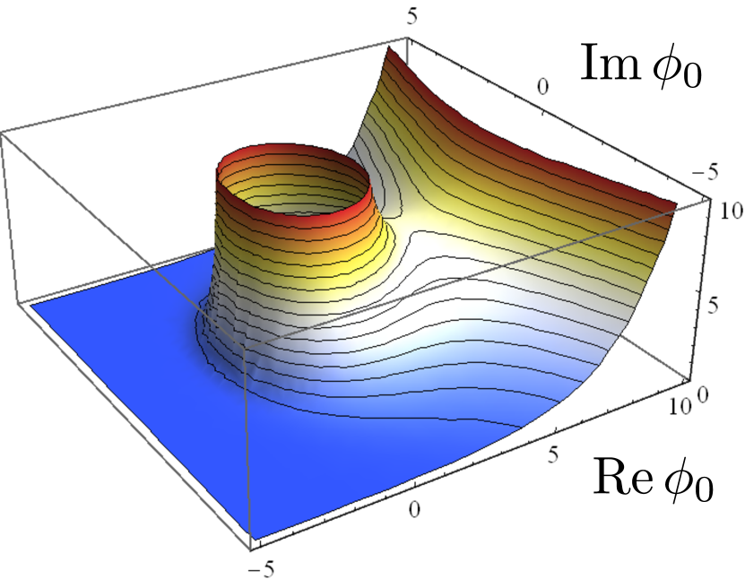
Figure 9: Modulus of $\phi_{0}^{-N_{0}}\exp(\phi_{0})$ for $N_{0}=5$, indicating the saddle point at $\phi_{0}=5$: the path of steepest descent through this point lies parallel to the imaginary axis.

Clearly, it is sensible to place the contour $C$ along the path of steepest descent through the saddle point and then to complete the circuit around the origin through regions where the modulus of the integrand is small. The contour integral is approximated by the contribution along a line parallel to the imaginary axis through $\phi_{0}=N_{0}.$ Writing $\phi_{0}=N_{0}+iy$ we have

$$\overline{N}\approx\exp\left(\ln F(N_{0})\right)$$ (93)

$$\times\int_{-\infty}^{\infty}i\,dy\frac{N_{0}!}{2\pi i}\exp\left(q(N_{0})+\frac{1}{2}q^{\prime\prime}(N_{0})(\phi_{0}-N_{0})^{2}\right)$$

$$\approx\frac{N_{0}!}{2\pi}\langle\phi\rangle_{N_{0}}N_{0}^{-1}\int_{-\infty}^{\infty}dy\>e^{N_{0}-N_{0}\ln N_{0}+(iy)^{2}/(2N_{0})}$$

$$\approx\langle\phi\rangle_{N_{0}}N_{0}!\left(\frac{N_{0}}{2\pi}\right)^{1/2}\frac{\exp(N_{0})}{N_{0}^{N_{0}+1}}\approx\langle\phi\rangle_{N_{0}},$$

using $n!\approx n^{n}\exp(-n)(2\pi n)^{1/2}$ which is quite accurate even for $N_{0}$ as low as unity. Finally, the expansion (23) with the $C_{j}(t)$ valid for $\kappa t\ll 1$ may be written

$$\langle\phi\rangle_{\phi_{0}}\approx\sum_{j=1}^{\infty}(-\kappa t)^{j-1}\phi_{0}^{j}=\frac{\phi_{0}}{1+\kappa\phi_{0}t},$$ (94)

making Eq. (93) and hence Eq. (92) consistent with the mean field approximation $\overline{N}\approx N_{0}/(1+\kappa N_{0}t)$ for small $\kappa t$.

Appendix E Equivalence of Drummond gauging and the Cameron-Martin-Girsanov formula

The equivalence between the statistical properties of the gauged stochastic variable $\phi^{\prime}$, when suitably weighted, and those of the ungauged variable $\phi$, derived by Drummond Drummond (2004) and explored in Section III.2, is a consequence of some fundamental rules in stochastic calculus that are expressed by the Cameron-Martin-Girsanov formula Cameron and Martin (1944, 1945); Girsanov (1960); Baxter and Rennie (1996). An SDE such as

$$dx=adt+bdW_{t},$$ (95)

is a statement of a connection between $dx$ and a stochastic variable $dW_{t}$ with certain statistical properties. When we evaluate expectation values such as $\langle dx\rangle$ we are implicitly defining a probability distribution or measure over the values taken by the variable $dW_{t}$. Normally the notation $dW_{t}$ represents an increment in a Wiener process and the implication is that the probability distribution of values of $dW_{t}$ is gaussian with zero mean and variance equal to $dt$.

But how might the expectation value of the increment $dW_{t}$ change if we were to evaluate it with respect to a different probability distribution? For example, what if it were distributed according to a shifted gaussian proportional to $\exp\left(-(dW_{t}-m)^{2}/\left(2dt\right)\right)$ where $m$ is the non-zero mean of $dW_{t}$ making it no longer an increment in a Wiener process? Let us take the mean of $dW_{t}$ under such a shifted gaussian distribution to be proportional to the time elapsed, such that we write $m=\mu dt$ and $\langle dW_{t}\rangle_{Q}=\mu dt$. The new probability distribution, denoted $Q$, is indicated through a suffix on the expectation value. We write $\langle dW_{t}\rangle_{P}=0$ in the old measure which we denote $P$, according to which $dW_{t}$ is indeed an increment in a Wiener process.

Note that $\langle dW_{t}-\mu dt\rangle_{Q}=0$ and $\langle\left(dW_{t}-\mu dt\right)^{2}\rangle_{Q}=dt$ since the variance of $dW_{t}$ under measure $Q$ is the same as that under $P$: we have shifted the gaussian probability distribution for $dW_{t}$ but not changed its width. Hence, if we define $d\tilde{W_{t}}=dW_{t}-\mu dt$ then $\langle d\tilde{W}_{t}\rangle_{Q}=0$ and $\langle(d\tilde{W}_{t})^{2}\rangle_{Q}=dt$: we can therefore identify a Wiener process that operates under probability measure $Q$, and relate it to a Wiener process under measure $P$. The SDE for $x$ now reads

$$dx=(a+b\mu)dt+bd\tilde{W}_{t},$$ (96)

and we can choose to evaluate expectation values under measure $P,$ for which $\langle d\tilde{W}_{t}\rangle_{P}=-\mu dt$, or measure $Q,$ for which $\langle d\tilde{W}_{t}\rangle_{Q}=0$.

The expectation value $\langle dx\rangle_{Q}$ is the solution to a problem that differs from the one initially posed, since the drift term in the SDE has been changed from $adt$ to $(a+b\mu)dt$. However, the point is that it is possible to establish a link between expectation values under the two different measures. The average of $dx$ under measure $P$ is equal to a weighted average of $dx$ under $Q$. Formally, we can write

$$\langle dx\rangle_{P}=\left\langle\frac{dP}{dQ}dx\right\rangle_{Q},$$ (97)

where $dP/dQ$ is the Radon-Nikodym derivative of probability measure $P$ with respect to $Q$. Furthermore, the Cameron-Martin-Girsanov formula states that we can write

$$\frac{dP}{dQ}=\exp\left(-\mu d\tilde{W}_{t}-\frac{1}{2}\mu^{2}dt\right),$$ (98)

which is just a ratio of the gaussian distributions $\exp[-(d\tilde{W}_{t}+\mu dt)^{2}/\left(2dt\right)]$ and $\exp[-d\tilde{W}_{t}{}^{2}/\left(2dt\right)]$. We now define a quantity $\Omega$ through the relation $\exp(d\ln\Omega)=dP/dQ$ such that

$$d\ln\Omega=-\mu^{2}dt/2-\mu d\tilde{W}_{t},$$ (99)

and using Ito’s lemma, it can be shown that $\Omega$ evolves according to

$$d\Omega=d\exp\left(\ln\Omega\right)=\exp\left(\ln\Omega\right)d\ln\Omega+\frac{1}{2}\exp\left(\ln\Omega\right)\mu^{2}dt$$ (100)

$$=\Omega\left(-\mu^{2}dt/2-\mu d\tilde{W}_{t}+\mu^{2}dt/2\right)=-\mu\Omega d\tilde{W}_{t}.$$

We see from Eqs. (97-100) that averages of the increment $dx$ over differently distributed random increments can be related to one another, and that the quantity $d\Omega$ describes the connection. In order for this to make sense mathematically, two conditions must be met. The first is that no process that has non-zero probability under $P$ should be impossible under $Q$, and vice versa. The second, known as Novikov’s condition, requires that $\left\langle\exp\left(\frac{1}{2}\mu^{2}dt\right)\right\rangle<\infty$.

We now invert the point of view, and instead of considering an increment of a variable treated according to two different averaging procedures, we relate increments of two different variables under the same averaging. Explicitly, we consider variable $x$ evolving as $dx=adt+bdW_{t}$ and another variable $x^{\prime}$ that evolves according to $dx^{\prime}=(a+b\mu)dt+bdW_{t}$, with $x(0)=x^{\prime}(0)$. The above results imply that we can write

$$\langle dx\rangle=\langle\exp(-\mu^{2}dt/2-\mu dW_{t})dx^{\prime}\rangle,$$ (101)

which resembles a combination of Eqs. (97) and (98). We shall demonstrate its validity shortly. Note that there is an implied suffix $P$ on the brackets, since $dW_{t}$ is here a standard Wiener increment with zero mean. The factor inserted in front of $dx^{\prime}$ accounts for the difference in drift in the evolution of $x$ and $x^{\prime}$ and may also be written $\exp(d\ln\Omega)$ with $d\ln\Omega=-\mu^{2}dt/2-\mu dW_{t}$ or equivalently $d\Omega=-\mu\Omega dW_{t}$. Clearly we can write $\exp(\int d\ln\Omega)=\exp[\ln\Omega(t)-\ln\Omega(0)]=\Omega(t)/\Omega(0)$ and if we set $\Omega(0)=1$ then

$$\Omega(t)=\exp\left(-\frac{1}{2}\int_{0}^{t}\mu^{2}(t^{\prime})dt^{\prime}-\int_{0}^{t}\mu(t^{\prime})dW_{t^{\prime}}\right).$$ (102)

Note that $\langle\Omega\rangle=\Omega(0)+\int\langle d\Omega\rangle=1-\int\langle\mu\Omega dW_{t}\rangle=1$. And for a finite interval of time, Novikov’s condition on $\mu$ reads $\left\langle\exp\left(\frac{1}{2}\int_{0}^{t}\mu^{2}(t^{\prime})dt^{\prime}\right)\right\rangle<\infty$.

Now consider the following:

$$\left\langle\Omega(t)\left(x^{\prime}(t)-x^{\prime}(0)\right)\right\rangle$$ (103)

$$=\left\langle\prod_{i}e^{-\frac{1}{2}\mu^{2}(t_{i})dt-\mu(t_{i})dW_{i}}\sum_{j}dx_{j}^{\prime}\right\rangle$$

$$=\sum_{j}\left\langle e^{-\frac{1}{2}\mu^{2}(t_{j})dt-\mu(t_{j})dW_{j}}dx_{j}^{\prime}\right\rangle,$$

where we use a discrete representation of the time integration. In deriving this we have recognised that if $k\neq j$ then

$$\!\!\!\left\langle\!\!e^{-\frac{1}{2}\mu^{2}(t_{k})dt-\mu(t_{k})dW_{k}}\prod_{i\neq k}e^{-\frac{1}{2}\mu^{2}(t_{i})dt-\mu(t_{i})dW_{i}}dx_{j}^{\prime}\right\rangle$$ (104)

$$=\left\langle e^{-\frac{1}{2}\mu^{2}(t_{k})dt-\mu(t_{k})dW_{k}}\right\rangle\left\langle\prod_{i\neq k}e^{-\frac{1}{2}\mu^{2}(t_{i})dt-\mu(t_{i})dW_{i}}dx_{j}^{\prime}\right\rangle$$

$$=\left\langle\prod_{i\neq k}e^{-\frac{1}{2}\mu^{2}(t_{i})dt-\mu(t_{i})dW_{i}}dx_{j}^{\prime}\right\rangle,$$

such that by repetition of this step, the right hand side reduces to $\left\langle\exp[-\frac{1}{2}\mu^{2}(t_{j})dt-\mu(t_{j})dW_{j}]dx_{j}^{\prime}\right\rangle$.

Using $\langle\exp\left(-\mu dW_{t}\right)\rangle=\exp(\mu^{2}dt/2)$ we can write

$$\left\langle\exp\left(-\mu dW_{t}\right)dW_{t}\right\rangle = -d\left\langle\exp\left(-\mu dW_{t}\right)\right\rangle/d\mu$$ (105)

$$= -\mu dt\,\exp(\mu^{2}dt/2),$$

and with the insertion of $dx^{\prime}=(a+b\mu)dt+bdW_{t}$, we conclude that

$$\left\langle e^{-\frac{1}{2}\mu^{2}(t_{j})dt-\mu(t_{j})dW_{j}}dx_{j}^{\prime}\right\rangle=$$ (106)

$$\left(a(t_{j})+b\mu(t_{j})\right)dt-b\mu(t_{j})dt=a(t_{j})dt=\langle dx_{j}\rangle,$$

such that

$$\!\left\langle\Omega(t)\!\left(x^{\prime}(t)-x^{\prime}(0)\right)\right\rangle=\sum_{j}\langle dx_{j}\rangle=\left\langle x(t)-x(0)\right\rangle,$$ (107)

and since

$$\left\langle\Omega(t)x^{\prime}(0)\right\rangle=\left\langle\Omega(t)\right\rangle\left\langle x^{\prime}(0)\right\rangle=\left\langle x(0)\right\rangle,$$ (108)

this means that

$$\langle x(t)\rangle=\left\langle\Omega(t)x^{\prime}(t)\right\rangle.$$ (109)

Thus we have shown that if we wish to evaluate the quantity $\langle x(t)\rangle$ generated by SDE $dx=adt+bdW_{t}$, we could instead solve the SDEs

$$dx^{\prime} = adt+b(dW_{t}-gdt)$$

$$d\Omega = g\Omega dW_{t},$$ (110)

with initial conditions $x^{\prime}(0)=x(0)$, $\Omega(0)=1$, and with the function $g(t)=-\mu(t)$ taking arbitrary form subject to Novikov’s condition, and then use the results to evaluate the equivalent quantity $\langle\Omega(t)x^{\prime}(t)\rangle$. Clearly, this is identical to Drummond’s gauging scheme.

References

• Smoluchowski (1906) M. Smoluchowski, Ann. Physik (Leipzig) 21, 756 (1906).
• Leyvraz (2003) F. Leyvraz, Phys. Rep. 383, 95 (2003).
• Lushnikov (2006) A. A. Lushnikov, Physica D 222, 37 (2006).
• Pruppacher and Klett (1997) H. R. Pruppacher and J. D. Klett, Microphysics of Clouds and Precipitation (Kluwer Academic, Boston, 1997).
• Mehlig and Wilkinson (2004) B. Mehlig and M. Wilkinson, Phys. Rev. Lett. 92, 250602 (2004).
• McGraw and Liu (2006) R. McGraw and Y. Liu, Geophys. Res. Lett. 33, L03802 (2006).
• Spicer and Pratsinis (1996) P. T. Spicer and S. E. Pratsinis, AIChE Journal 42, 1612 (1996).
• Lushnikov (1978) A. A. Lushnikov, J. Colloid Interface Sci. 65, 276 (1978).
• Lushnikov (2005) A. A. Lushnikov, J. Phys. A: Math. Gen. 38, L383 (2005).
• Krug (2003) J. Krug, Phys. Rev. E 67, 065102(R) (2003).
• Smith and Matsoukas (1998) M. Smith and T. Matsoukas, Chem. Eng. Sci. 53, 1777 (1998).
• Hendriks et al. (1985) E. M. Hendriks, J. L. Spouge, M. Eibl,  and M. Schreckenberg, Z. Phys. B - Condensed Matter 58, 219 (1985).
• Doi (1976a) M. Doi, J. Phys. A: Math. Gen 9, 1465 (1976a).
• Doi (1976b) M. Doi, J. Phys. A: Math. Gen 9, 1479 (1976b).
• Peliti (1985) L. Peliti, J. de Phys. 46, 1469 (1985).
• Patzlaff et al. (1994) H. Patzlaff, S. Sandow,  and S. Trimper, Z. für Phys. B 95, 357 (1994).
• Rey and Droz (1997) P.-A. Rey and M. Droz, J. Phys. A: Math. Gen. 30, 1101 (1997).
• Mattis and Glasser (1998) D. C. Mattis and M. L. Glasser, Rev. Mod. Phys. 70, 979 (1998).
• Sasai and Wolynes (2003) M. Sasai and P. G. Wolynes, Proc. Nat. Acad. Sci. USA 100, 2374 (2003).
• Täuber et al. (2005) U. C. Täuber, M. Howard,  and B. P. Vollmayr-Lee, J. Phys. A: Math. Gen. 38, R79 (2005).
• Ohkubo (2007a) J. Ohkubo, J. Stat. Mech.: Theory Exp. P09017  (2007a).
• Schulz (2008) M. Schulz, Eur. Phys. J. Special Topics 161, 143 (2008).
• Ohkubo (2007b) J. Ohkubo, Phys. Rev. E 83, 041915 (2007b).