Modified Rindler acceleration as a nonlinear electromagnetic effect

Abstract

The model proposed originally by Mannheim and Kazanas for fitting the shapes of galactic rotation curves has recently been considered by Grumiller to describe gravity of a central object at large distances. Herein we employ the same geometry within the context of nonlinear electrodynamics (NED). Pure electrical NED model is shown to generate the novel Rindler acceleration term in the metric which explains anomalous behaviors of test particles / satellites. Remarkably a pure magnetic model of NED yields flat rotation curves that may account for the missing dark matter. Weak and Strong Energy conditions are satisfied in such models of NED.

I INTRODUCTION

In Newton’s theory of gravitation which reined for centuries, mass constituted the principal source for its potential. With the advent of general relativity, different sources were unified under spacetime texture such that the overall effective force used to matter. Thus, gravity / geometry can easily be attributed to non-mass originated sources equally well due to the manifestation of mass-energy equivalence. As a particular example we recall the Reissner-Nordström (RN) geometry of general relativity in which mass and charge coexist in making the geometry. Assuming that the source has negligible mass versus a significant charge the entire geometry can be attributed to the charge alone. In performing this process one should be cautious that no physical energy conditions are violated. Recent observations suggest that there are dark matter / energy that is associated with non-observable sources. As a result our detectable / observable matter falls rather short to account for the accelerated expansion of our universe.  Before suggesting proposals for new forces / matter it is more logical to exhaust every kind of physical sources that we are at least familiar so that we know how to cope with. To explain the hierarchy of forces at small distances and close the gap of discrepancy between gravity and other fields , for instance, the idea of higher dimensions / branes was proposed 1 ; 2 . Although no branes have been identified so far theoretical explanation such as dilution (weaking) of gravity among branes in higher dimensions remains consistently intact. As the gravity is tamed at UV scales by virtue of higher dimensions at the IR scales, or long distances does everything go perfect?. The recent proposal 3 ; 4 ; 5 ; 6 that at large distances there is an additional parameter known as Rindler acceleration was rather unprecedented and the present paper is about the source of such a term.

We recall that in the near horizon limit, i.e. $r=2m+x$ for $\left|x\right|^{2}\ll 1,$ a Schwarzschild black hole leads to the standard Rindler acceleration. Such an extraneous term must be purely general relativistic coupled with physical sources which lacks a Newtonian counterpart. Even in the Einstein-Maxwell version of general relativity with spherical symmetry such a term did not arise. The long range fields, i.e. gravitation and electromagnetism, manifest their inverse square law character so that asymptotically the spacetime becomes flat. Different sources such as dilatons, nonlinear electromagnetic fields and others admit non asymptotically flat solutions at large spatial distances. The difficulty with the new Rindler acceleration is that it violates both the Newtonian and Maxwellian limits: for large distances ($r\rightarrow\infty$) it becomes even more significant. In Newtonian terms the potential that gives inverse force law modifies into $\phi\left(r\right)=-\frac{m}{r}+ar$, where $m$ is the central Newtonian mass and $a$ is the novel Rindler acceleration under question. Unless the central object is supermassive and $a$ is negligibly small it can be argued that for large $r$ the new term dominates over the mass term. Further, the Rindler acceleration is not a universal constant as observationally it shows slight variations from Sun-Pioneer pair ($\sim 10^{-61}$ natural unit of acceleration which is equivalent to $10^{-10}\frac{m}{s^{2}}$ in physical units) to galaxy-Sun system ($\sim 10^{-62}$) and others. We recall that such a linear dependence of potential on distance is encountered in parallel plates endowed with a uniform electric field in linear Maxwell electromagnetism (i.e. $V_{0}=E_{0}z$, $E_{0}=$ constant).

Gravity coupled with linear Maxwell electromagnetism in spherically symmetric geometry produces no such linear potential term either. For this reason we resort from the outset to nonlinear electrodynamics (NED) and prove a theorem to generate the new acceleration term. Truly it yields the required expression, however, in addition it gives as a by product an extra constant term in the metric which can be interpreted as a global monopole 7 ; 8 . This amounts to further modification of the Newtonian potential by $\phi\left(r\right)=k-\frac{m}{r}+ar$, with the global monopole term  $k=$ constant. Our formalism suggests that both the Rindler acceleration ($a$) and global monopole ($k$) constants depend on the nonlinear electric charge of the heavenly object under consideration. That is, neither one is a fundamental constant of nature as both are derived from the charge. Interestingly the monopole term plays the similar role of a cosmological constant, i.e. a uniform electric field in the presence of NED-coupled gravity with nonisotropic difference. The upper bounds for both $\left|a\right|$ and $\left|k\right|$ have been tabulated for different planets. It is further shown that the monopole term is crucial for the weak and strong energy conditions to be satisfied. The spectrum of NED theories is very large and the problem is to find the proper Lagrangian that suits and serves for the purpose. Finally we observed that the Rindler acceleration doesn’t account for the constant tangential velocity of circular orbits in the presence of mysterious dark matter. For this reason we have further modified the Rindler term in the metric function by $2ar\rightarrow 2ar_{0}\ln r$ (with $a$ and $r_{0}$ constant), which necessitates a new NED Lagrangian. For such a magnetic Lagrangian it is shown that the energy conditions are satisfied at the cost of a bounded universe. Further, the circular orbit around remote galaxies, has velocity $v=\sqrt{\frac{m}{r}+ar_{0}}$ which yields a better estimate between Newton and Rindler acceleration models toward accounts of dark matter.

II The Solutions

II.1 Pure Electric case

Recently, Grumiller considered the Mannheim-Kazanas (MK) metric to describe gravity of a central mass at large distances which attracted interest due to its cosmological implications 5 ; 6 . We must add that a linear term in the metric was first introduced in 3 , and it was applied in earnest in fitting the shapes of galactic rotation curves by Mannheim (see 4 , for a review). The novelty in this model is the inclusion of a term interpreted as Rindler acceleration. We wish to show in this paper that nonlinear electrodynamics (NED) may be responsible for the generation of such a term. Our starting point is the action

$$S=\int d^{4}x\sqrt{-g}\left[R-2\Lambda+L\left(\mathcal{F}\right)\right]$$ (1)

in which $R=$ Ricci scalar, $\Lambda=$ cosmological constant and $L\left(\mathcal{F}\right)$ is the Lagrangian for the NED.

Before we choose the form of $L\left(\mathcal{F}\right)$ we would like to add that $L\left(\mathcal{F}\right)$ is not similar to the original BI Lagrangian. In Born-Infeld (BI) initial work the idea was the removal of the singularity at the origin. Following the classical charge with a finite size and a well defined charge distribution admitted what we call it BI Lagrangian. In what we introduce the singularity at the origin is not our worry any more and instead we are adjusting our Lagrangian to justify the behavior of the Galaxies at very large distance. Hence, the only constraint we impose on our Lagrangian is to satisfy the Maxwell equation with a single electric or magnetic fields. No need to mention that such an arbitrary Lagrangian may not give the Maxwell limit at large distance which otherwise expecting the Mannheim-Kazanas instead of Reissner-Nordström would be meaningless.

Our notation is such that $\mathcal{F}=F_{\mu\nu}F^{\mu\nu\text{ }}$ represents the Maxwell invariant with the choice of Lagrangian

$$L\left(\mathcal{F}\right)=\frac{\alpha}{\sqrt{2}\beta-\sqrt{-\mathcal{F}}}.$$ (2)

Here $\alpha>0$ is the coupling constant and $\beta>0$ plays the role of the uniform background electric field as will be clarified in the sequel. Our original model Lagrangian (2) can be employed with the choice $\beta=0$ as well. Note that $F_{\mu\nu}=\partial_{\mu}A_{\nu}-\partial_{\nu}A_{\mu}$ is the standard Maxwell field tensor and this Lagrangian will break the scale invariance, i.e. $x\rightarrow\lambda x,$ $A_{\mu}\rightarrow\frac{1}{\lambda}A_{\mu},$ for $\lambda=$ constant. We consider a static, spherically symmetric (SSS) spacetime described by the line element

$$ds^{2}=-f(r)dt^{2}+\frac{dr^{2}}{f(r)}+r^{2}\left(d\theta^{2}+\sin^{2}\theta d\phi^{2}\right),$$ (3)

with the electric field ansatz.

The fact that the desired static spherically symmetric (SSS) line element (3) derives from the NED Lagrangian (2) through the action (1) can be formulated as a theorem 9 .

Theorem: Let our action be (1) with line element (3) and $L(F)$ be our pure electric NED Lagrangian described by the Maxwell $2-$form

$$\mathbf{F}=E\left(r\right)dt\wedge dr$$ (4)

satisfying the Maxwell’s equation

$$d\left({}^{\star}\mathbf{F}L_{\mathcal{F}}\right)=0$$ (5)

in which ${}^{\star}\mathbf{F}$ means dual of $\mathbf{F}$ and $L_{\mathcal{F}}=\frac{\partial L}{\partial\mathcal{F}}.$ Then, the energy-momentum tensor satisfies the conditions $T_{t}^{t}=T_{r}^{r}$ and $T_{\theta}^{\theta}=T_{\varphi}^{\varphi}$ and Lagrangian $L(\mathcal{F})$ is related to the metric function $f(r)$ through

$$L=L_{0}+2\int\frac{1}{r^{2}}\left[r^{2}\left(\frac{f^{\prime\prime}}{2}+\frac{1-f}{r^{2}}\right)\right]^{\prime}dr$$ (6)

where $L_{0}=const.$ and a ’prime’ implies $\frac{d}{dr}.$

Proof: Variation of the action (1) with respect to the metric tensor $g_{\mu\nu}$ yields the field equations in the form

$$G_{\mu}^{\nu}+\Lambda\delta_{\mu}^{\nu}=T_{\mu}^{\nu}$$ (7)

where $G_{\mu}^{\nu}$ is the Einstein tensor and $T_{\mu}^{\nu}$ is the energy-momentum tensor given by

$$T_{\mu}^{\nu}=\frac{1}{2}\left(L\delta_{\mu}^{\nu}-4L_{\mathcal{F}}F_{\mu\lambda}F^{\nu\lambda}\right)$$ (8)

which admits $T_{t}^{t}=T_{r}^{r}=\frac{1}{2}L-\mathcal{F}L_{\mathcal{F}}$ and $T_{\theta}^{\theta}=T_{\varphi}^{\varphi}=\frac{1}{2}L.$ From the line element (3) we find

$$G_{t}^{t}=G_{r}^{r}=\frac{rf^{\prime}-1+f}{r^{2}}$$ (9)

and

$$G_{\theta}^{\theta}=G_{\varphi}^{\varphi}=\frac{rf^{\prime\prime}+2f^{\prime}}{2r}.$$ (10)

The electric field $2-$form has the dual given by

$${}^{\star}\mathbf{F}=-E\left(r\right)r^{2}\sin\theta d\theta\wedge d\varphi$$ (11)

and the Maxwell’s equation (5) implies that

$$E\left(r\right)r^{2}L_{\mathcal{F}}=const.=Q$$ (12)

in which $Q$ is a charge related integration constant. Recall that, $L_{\mathcal{F}}=\frac{\partial L}{\partial\mathcal{F}}=\frac{L_{E}}{\frac{\partial\mathcal{F}}{\partial E}}$ and since $\mathcal{F}=-2E^{2},$ we have $L_{\mathcal{F}}=-\frac{L_{E}}{4E}.$ Comparing this with Eq. (12) yields

$$L_{E}=\frac{-4Q}{r^{2}}.$$ (13)

From (7) we have $G_{t}^{t}=T_{t}^{t}-\Lambda,$ which reads

$$\frac{rf^{\prime}-1+f}{r^{2}}=\frac{1}{2}L-\mathcal{F}L_{\mathcal{F}}-\Lambda$$ (14)

or alternatively

$$\frac{rf^{\prime}-1+f}{r^{2}}=\frac{1}{2}\left(L+\frac{4QE}{r^{2}}\right)-\Lambda.$$ (15)

The other field equation $G_{\theta}^{\theta}=T_{\theta}^{\theta}-\Lambda$ reads as

$$\frac{rf^{\prime\prime}+2f^{\prime}}{2r}=\frac{1}{2}L-\Lambda.$$ (16)

Next, we subtract (16) from (15) which determines the electric field

$$E=-\frac{r^{2}}{2Q}\left(\frac{f^{\prime\prime}}{2}+\frac{1-f}{r^{2}}\right).$$ (17)

Note that from the chain rule we have

$$\frac{dL}{dr}=-\frac{4Q}{r^{2}}\frac{dE}{dr}.$$ (18)

Using (17) and the latter relation one finds

$$\frac{dL}{dr}=\frac{2}{r^{2}}\left[r^{2}\left(\frac{f^{\prime\prime}}{2}+\frac{1-f}{r^{2}}\right)\right]^{\prime}$$ (19)

or consequently

$$L=L_{0}+2\int\frac{1}{r^{2}}\left[r^{2}\left(\frac{f^{\prime\prime}}{2}+\frac{1-f}{r^{2}}\right)\right]^{\prime}dr$$ (20)

which completes the proof.

Now we apply the theorem for the MK metric which admits $L\sim\frac{1}{\sqrt{-\mathcal{F}}}$. Next, to make our study more general, we modify this Lagrangian as given in Eq. (2). The nonlinear Maxwell equation $d\left({}^{\star}\mathbf{F}\frac{\partial L}{\partial\mathcal{F}}\right)=0,$ admits the electric field

$$E(r)=E_{0}-\xi r$$ (21)

in which $E_{0}=const.(=\beta)$ and $\xi=2^{-5/4}\sqrt{\frac{\alpha}{C}}=const.$ We note that the integration constant $C$ is identified as the total charge $Q$ of the central object which is obtained from the Gauss’s law $\oint\left({}^{\star}\mathbf{F}\frac{\partial L}{\partial\mathcal{F}}\right)=4\pi Q.$ The solution of Einstein-NED equations gives the following metric function

$$f(r)=1+2k-\frac{2m}{r}+2ar-\frac{1}{3}\Lambda r^{2},$$ (22)

where $k=-QE_{0}=const.<0$, $a=2^{-5/4}\sqrt{\alpha Q}=const.$ while $m=$ mass and $\Lambda=$ the cosmological constant, require no comments. As the expressions suggest $\alpha$ and $Q$ must have the same sign and the fact that the acceleration admits both signs has cosmological implications. If this metric is compared with MK one, it can be easily seen that the Rindler’s acceleration constant is derived from the charge $Q$. Beside this acceleration we have an additional constant $k=QE_{0}$ which can be interpreted as a global monopole term 7 ; 8 . The global monopole charge is identified as $\eta=\pm\sqrt{\left|\frac{QE_{0}}{4\pi}\right|}$ which gives rise to non-radial stresses. Let us add that $Q$ and $E_{0}$ are both small enough to elude experimental observations. It’s origin can be traced back to big bang as a topological defect. Being coupled to the distance $\sim r$ from the center of attraction, however,  enhances its role at large distances. We recall that the cosmological constant $\Lambda$ is also very small but it couples with $\sim r^{2}$ in the metric to account for a significant effect. Naturally such a monopole charge modifies the Newtonian potential by $\Phi\left(r\right)=k-\frac{m}{r},$ which violates asymptotic flatness. In case that $Q\rightarrow 0$ the line element reduces to the standard Schwarzschild-de Sitter, as it should be. The essential parameters of our model consist of $Q,$ $E_{0},$ $m$ and $\Lambda$ (or $k$). With the choice $\beta=0$ the uniform electric field $E_{0}$ will not exist any more. To what extent our model is physical?. Satisfaction of the energy conditions are vitally important for a physically acceptable solution. Let us note that in the original MK’s model unless $a<0$ the energy conditions are violated. In the present case with the NED as source we wish to show that the energy conditions are satisfied. To illustrate this we explicitly present the corresponding energy momentum tensor as follows

$$T_{\mu}^{\nu}=\text{diag}\left[-\rho,p_{r},p_{\theta},p_{\phi}\right]=\frac{2a}{r}\text{diag}\left[2+\frac{k}{ar},2+\frac{k}{ar},1,1\right].$$ (23)

The weak energy condition (WEC) requires that $\rho\geq 0,$ and $\rho+p_{i}\geq 0.$ For the strong energy condition (SEC),  in addition to WEC, we must have $\rho+\sum\limits_{i=1}^{3}p_{i}\geq 0.$ These conditions are both satisfied provided that

$$2ar\leq\left|k\right|$$ (24)

for our choice of $E_{0}>0$, $Q>0$ so that $k<0$ and $a>0.$ This suggests that validity of the energy conditions confines the motion by $E_{0}$ and the Rindler acceleration $a.$ The fact that $a$ is very small ($\simeq 10^{-10}\frac{m}{s^{2}}$) makes $r$ from (24) still quite large. $E_{0}$ can be interpreted as a uniform background electric field filling all space which appears also in the Lagrangian (i.e. $E_{0}=\beta$). This makes $E_{0}$ an indispensable parameter of the theory provided we stipulate the energy conditions. Once we set $E_{0}=\beta=0,$ the nonlinear Lagrangian reduces to $L\left(\mathcal{F}\right)=\frac{-\alpha}{\sqrt{-\mathcal{F}}}$ with the solution for the electric field $E(r)=-\xi r,$ ($\xi=const.$). However, this will violate the energy conditions and due to this fact, we are compelled to invoke a space filling uniform electric field $E_{0}$ as regulator, much like the concept of cosmological constant $\Lambda.$ All galaxies must be considered immersed in such a background $E_{0}$ to regulate energy conditions. Although locally $E_{0}$ is too small to be detected globally it effects the geodesics. (This can best be seen from the above definitions where $\left|E_{0}\right|=\frac{\left|k\alpha\right|}{a^{2}},$ which can be made arbitrarily small with the weaker coupling parameter $\alpha$).

The role of $E_{0}$ becomes even more transparent if we assume the central object to host a black hole. The horizon radius shows a steep rise versus $E_{0}$ and the Hawking temperature $T_{H}$ which depends also on the Rindler acceleration reaches saturation for increasing $E_{0}$. That is, no matter how $E_{0}$ rises, $T_{H}$ reaches a constant value above zero. From the thermodynamical point of view, $k=\frac{1}{2}$ acts as a point of phase transition. From physical standpoints the global monopole parameter, $\left|k\right|=$ $QE_{0}$ may be chosen small enough, apt for perturbative treatment. This is not imperative however, since relaxation of this condition will naturally yield from the geodesics equation open, hyperbolic orbits admissible as well. Global monopoles are known to arise also in modified $f(R)$ theories 7 .

The equation of motion for a charged test particle is given by

$$\dot{r}^{2}+V_{eff}(r)=\mathcal{E}^{2}$$ (25)

in which the ’dot’ stands for derivative with respect to proper time and the effective potential reads

$$V_{eff}(r)=q_{0}r\left(E_{0}+\frac{\xi}{2}r\right)\left[2\mathcal{E-}q_{0}r\left(E_{0}+\frac{\xi}{2}r\right)\right]+f(r)\left(1+\frac{\ell^{2}}{r^{2}}\right).$$ (26)

Here $\mathcal{E}$ ($=$ energy) and $\ell$ ($=$ angular momentum) are the constants of motion while $q_{0}$ is the charge of the test particle. The simplest way to handle this potential analytically is to consider a neutral ($q_{0}=0$) particle at larger $r$ with $\Lambda=0.$ The geodesics equation simplifies to $\dot{r}^{2}+\left(1+k+ar\right)\simeq\mathcal{E}^{2},$ which integrates to

$$r(\tau)=\frac{\mathcal{E}^{2}-k-1}{a}-\frac{3}{2}a^{-1/3}\left(\tau-\tau_{0}\right)^{2/3}.$$ (27)

It is observed that in this model there is not only a maximum radius (i.e. Eq. (24)) but also a maximum proper time determined by $\mathcal{E}^{2}/a$ and $\left|k\right|/a.$

The null geodesics equation for $u(\phi)=\frac{1}{r}$ reads 10 , for $\Lambda=0$

$$\frac{d^{2}u}{d\phi^{2}}+\left(1-2\left|k\right|\right)u=3mu^{2}-a$$ (28)

which upon scalings $\phi\rightarrow\sqrt{1-2\left|k\right|}\phi$, $m\rightarrow\frac{m}{1-2\left|k\right|}$ and $a\rightarrow\frac{a}{1-2\left|k\right|}$ the perturbative solution can be found. Employing $u=\frac{\sin\phi}{R},$ as the flat space solution with $R=$ the minimum light distance, the total bending angle for the photon orbit 10 modifies into

$$2\psi_{0}\approx\frac{4m}{R}\left[1+2ma+2\left|k\right|\left(1+6ma\right)\right].$$ (29)

II.1.1 Solar system upper bound for $\left|k\right|$

In this subsection we apply a similar calculation as in 6 to find an upper bound for the parameter $\left|k\right|$ and therefore for the background electric field. The effective potential for a particle in a stable circular motion is given by

$$V_{eff}=\frac{1}{2}\left[1+2k-\frac{2M}{r}+2ar\right]\left(1+\frac{\ell^{2}}{r^{2}}\right)$$ (30)

where at $r=r_{c}$ we have

$$\frac{dV_{eff}}{dr}=0$$ (31)

which implies

$$\ell^{2}=\frac{\left(M+ar_{c}^{2}\right)r_{c}^{2}}{-3M+ar_{c}^{2}+r_{c}+2kr_{c}}.$$ (32)

A small perturbation applied to the stable orbit of the particle will cause an oscillatory motion with the frequency

$$\omega_{r}=\left(\frac{d^{2}V_{eff}}{dr^{2}}\right)_{r_{c}}.$$ (33)

Since we are interested in the perihelion oscillation frequency it is given by

$$\omega_{p}=\frac{\ell^{2}}{r_{c}^{2}}-\omega_{r}$$ (34)

which up to the first order approximation it amounts to

$$\omega_{p}\simeq\frac{3M^{3/2}}{r_{c}^{5/2}}\left(1-\frac{r_{c}^{3}}{3M^{2}}a-k\left(\frac{13}{2}+\frac{r_{c}}{3M}\right)\right)$$ (35)

or in analogy with 5 ; 6 ; 11

$$\omega_{p}\simeq\frac{3M^{3/2}}{A^{5/2}\left(1-e^{2}\right)^{5/4}}\left(1-\frac{A^{3}\left(1-e^{2}\right)^{3/2}}{3M^{2}}a-k\left(\frac{13}{2}+\frac{A\sqrt{1-e^{2}}}{3M}\right)\right).$$ (36)

Herein $A$ stands for the semimajor axis of the ellipse and $e$ is its eccentricity. As it has been considered in 5 ; 6 the first term is just the perihelion frequency in general relativity (leading term). This means that the second and third terms represent the shift of the general relativity up to first order in $a$ and $k,$ respectively, i.e.,

$$\frac{\Delta\omega_{p}}{\omega_{p}}=\frac{A^{3}\left(1-e^{2}\right)^{3/2}}{3M^{2}}a+k\left(\frac{13}{2}+\frac{A\sqrt{1-e^{2}}}{3M}\right).$$ (37)

This in turn suggests that $\left|a\right|$ is bounded by

$$\left|a\right|<\frac{\Delta\omega_{p}}{\omega_{p}}\frac{3M^{2}}{A^{3}\left(1-e^{2}\right)^{3/2}}$$ (38)

and

$$\left|k\right|<\frac{\Delta\omega_{p}}{\omega_{p}}\frac{1}{\frac{13}{2}+\frac{A\sqrt{1-e^{2}}}{3M}}.$$ (39)

Tab. I shows a list of upper bounds for $\left|a\right|$ and $\left|k\right|$ for different planets which is consistent with 5 ; 6

Table 1: Upper bound for $\left|k\right|$ and $\left|a\right|.$ We note that the first and third rows are in natural units i.e., $c=G=\hbar=1.$

Planet	Mercury	Venus	Earth	Mars	Jupiter	Saturn	Uranus	Icarus
$\left|a\right|{\small<}$	${\small 2.82\times 10}^{-64}$	${\small 1.31\times 10}^{-65}$	${\small 1.65\times 10}^{-66}$	${\small 0.25\times 10}^{-66}$	${\small 0.94\times 10}^{-64}$	${\small 0.11\times 10}^{-65}$	${\small 0.42\times 10}^{-65}$	${\small 0.90\times 10}^{-62}$
$\left|a\right|\left(\frac{m}{s^{2}}\right){\small<}$	${\small 0.16\times 10}^{-12}$	$0.{\small 73\times 10}^{-13}$	$0.{\small 92\times 10}^{-14}$	${\small 0.14\times 10}^{-14}$	${\small 0.52\times 10}^{-12}$	${\small 0.61\times 10}^{-14}$	${\small 0.23\times 10}^{-13}$	${\small 0.50\times 10}^{-10}$
$\left|k\right|{\small<}$	${\small 0.48\times 10}^{-11}$	$0.{\small 71\times 10}^{-11}$	$0.{\small 15\times 10}^{-11}$	${\small 0.53\times 10}^{-12}$	${\small 0.26\times 10}^{-8}$	${\small 0.99\times 10}^{-10}$	${\small 0.15\times 10}^{-8}$	${\small 0.36\times 10}^{-8}$

To complete our calculation we used the data provided in 12 ; 13 ; 14 ; 15 ; 16 which are the updated version of those given in 16 ; 17 ; 18 ; 19 (Tab. II is the summary of these data).

Table 2: Perihelion precessions and the uncertainties taken from 12 ; 13 ; 14 ; 15 ; 20 .

Planet	Mercury	Venus	Earth	Mars	Jupiter	Saturn	Uranus	Icarus
$\delta\Delta\phi(^{\prime\prime}/cy)\sim\Delta\omega_{p}$	${\small 0.0030}$	${\small 0.0016}$	${\small 0.00019}$	${\small 0.000037}$	${\small 0.0283}$	${\small 0.00047}$	${\small 3.90}$	${\small 0.8}$
$\Delta\phi(^{\prime\prime}/cy)\sim\omega_{p}$	${\small 42.982}$	$8.646$	$3.84019$	${\small 1.35002}$	${\small 0.0587}$	${\small 0.01432}$	${\small 3.89}$	${\small 9.8}$

Concerning Tab. I it is seen that the smallest bound is given by Mars which is $\left|k\right|<0.{\small 53\times 10}^{-12}.$ It is remarkable to observe that this value of the lower bound for $\left|k\right|$ is much smaller than its typical value in grand unified theory $10^{-5}$ 9 . Also we add that $\left|k\right|$ is unit-less unlike $a$ which is in $m/s^{2}.$ In Refs. 20 ; 21 ; 22 , additional perihelion precessions such as the Lense-Thirring effect $\dot{\varpi}_{LT}$ 23 ; 24 , the supplementary rates $\Delta\dot{\varpi}$ and the second Post-Newtonian (2PN) perihelion precessions are discussed. One may disentangle these various contributions from the uncertainty given in Tab. II to find a finely tuned upper bound for the parameters $a$ and $k.$ For instance here we quote Tab. III from Ref. 21 together with our $\left|k\right|.$

Table 3: Additional perihelia precessions such as the Lense-Thirring effect $\dot{\varpi}_{LT}$, the supplementary rates $\Delta\dot{\varpi}$ and 2PN perihelion precessions quoted from 21 .

Planet	Mercury	Venus	Earth	Mars	Jupiter	Saturn
$\Delta\dot{\varpi}\left(mas/cy\right)$13 ; 25	${\small-2.0\pm 3.0}$	${\small 2.6\pm 1.6}$	${\small 0.19\pm 0.19}$	${\small-0.020\pm 0.037}$	${\small 58.7\pm 28.3}$	${\small-0.32\pm 0.47}$
$\dot{\varpi}_{LT}\left(mas/cy\right)$23	${\small-2.0}$	$-0.2$	$-0.09$	${\small-0.027}$	${\small-7\times 10}^{-4}$	$-1\times 10^{-4}$
$\dot{\varpi}_{2PN}\left(mas/cy\right)$26 ; 27	${\small 7\times 10}^{-3}$	$6\times 10^{-4}$	$2\times 10^{-4}$	${\small 6\times 10}^{-5}$	$9\times 10^{-7}$	$9\times 10^{-8}$
$\left|k\right|\left(\text{Natural units}\right)<$	${\small 0.48\times 10}^{-11}$	$0.71\times 10^{-11}$	$0.15\times 10^{-11}$	$0.53\times 10^{-12}$	$0.26\times 10^{-8}$	$0.99\times 10^{-10}$

After the corresponding subtraction or addition to what we found is given in Tab. III which is the same as given in Tab. I. The reason can be due to small corrections which has no significant effect in our approximation. Therefore using the updated data given in 12 ; 13 ; 14 ; 15 would be satisfactory to have a general idea of the upper bound for our parameters.

We note that the effects of a Pioneer-type / Rindler acceleration on the outer parts of the Solar System have been studied in 28 ; 29 ; 30 ; 31 . Also, the effect of a Pioneer-type acceleration on the perihelion of a planet was computed for the first time in 32 ; 33 ; 34 ; 35 .

II.2 Pure magnetic solution and modified MK metric

In this section we consider not exactly the MK metric but a modified version of it in which instead of a linear term we have a logarithmic term. As we shall show in the sequel, such a model admits a velocity-distance curve which may be closer to the observational data. In addition to that, we consider a pure magnetic field to be responsible for such logarithmic term via a non-linear electrodynamic Lagrangian which is not in the standard BI Lagrangian form but in a form which accommodate such extra term in the metric function. As we have mentioned in our previous section, our interest region is not close to the origin but far distance from the center of galaxies. In order to establish a pure magnetic solution of NED we start with the following NED Lagrangian

$$L\left(\mathcal{F}\right)=\alpha\sqrt{\mathcal{F}}\left(1-\frac{\ln\left(\frac{\mathcal{F}}{2}\right)}{4}\right)$$ (40)

where $\alpha>0$ is the coupling constant and $\mathcal{F}$ is the Maxwell invariant. Note that these constants are distinct from the ones given in (2). The vector potential is $A_{\mu}=\delta_{\mu}^{\varphi}P\cos\theta$ where $P>0$ is the magnetic charge so that

$$\mathcal{F}=F_{\mu\nu}F^{\mu\nu}=2\frac{P^{2}}{r^{4}}>0.$$ (41)

The energy momentum tensor’s components are given by (8) which explicitly becomes

$$T_{t}^{t}=T_{r}^{r}=\frac{\alpha\sqrt{2}P}{2r^{2}}\left(1-\ln\left(\frac{\sqrt{P}}{r}\right)\right)$$ (42)

and

$$T_{\theta}^{\theta}=T_{\phi}^{\phi}=\frac{\alpha\sqrt{2}P}{2r^{2}}.$$ (43)

Choosing SSS line element (3), the $tt$ component of the Einstein-NED equations with $\Lambda=0$ yields a solution of the form

$$f(r)=1-\frac{2m}{r}+\alpha\frac{\sqrt{2}P}{2}\ln\left(\frac{r}{\sqrt{P}}\right)$$ (44)

in which $m$ is an integration constant. Next, we introduce two new parameters as $r_{0}=\sqrt{P}$ and $a=\frac{\alpha\sqrt{P}}{2\sqrt{2}}$ and upon that the metric function is written as

$$f(r)=1-\frac{2m}{r}+2ar_{0}\ln\left(\frac{r}{r_{0}}\right).$$ (45)

We would like to comment that, expressing the metric function in latter form enables us to compare it to the standard form of the MK metric which in turn implies that $a$ is a similar parameter as Rindler acceleration.

It can be checked that the WEC and SEC are satisfied provided $r<\frac{r_{0}}{\sqrt{e}}.$ Naturally, in this model the galaxies can’t run out infinity. The Newtonian potential in this model modifies as

$$\Phi=-\frac{m}{r}+ar_{0}\ln\left(\frac{r}{r_{0}}\right)$$ (46)

so that the attractive force $\overrightarrow{F}=-\overrightarrow{\nabla}\Phi$ takes the form

$$\left|\overrightarrow{F}\right|=\frac{m}{r^{2}}+\frac{ar_{0}}{r}.$$ (47)

It worths to mention that a logarithmic potential yielding a $\frac{1}{r}$ extra-force, has been considered in 36 ; 37 in which it was applied to the Solar System. For circular orbits since $\left|\overrightarrow{F}\right|=\frac{v^{2}}{r}$ for a unit mass particle, this yields the velocity function as

$$v=\sqrt{\frac{m}{r}+ar_{0}}.$$ (48)

This differs from the Newtonian model ($v=\sqrt{\frac{m}{r}}$) and the model proposed by Grumiller ($v=\sqrt{\frac{m}{r}+ar}$) 5 . Evidently, for $r\rightarrow\infty$ our model has the advantage since $v\rightarrow cons.,$ which is the case believed to be in the presence of dark matter. Fig. 1 displays the three cases openly with the chosen mass and density functions as described below shortly. No doubt the gap between our model and Newtonian one corresponds to the invisible dark matter.

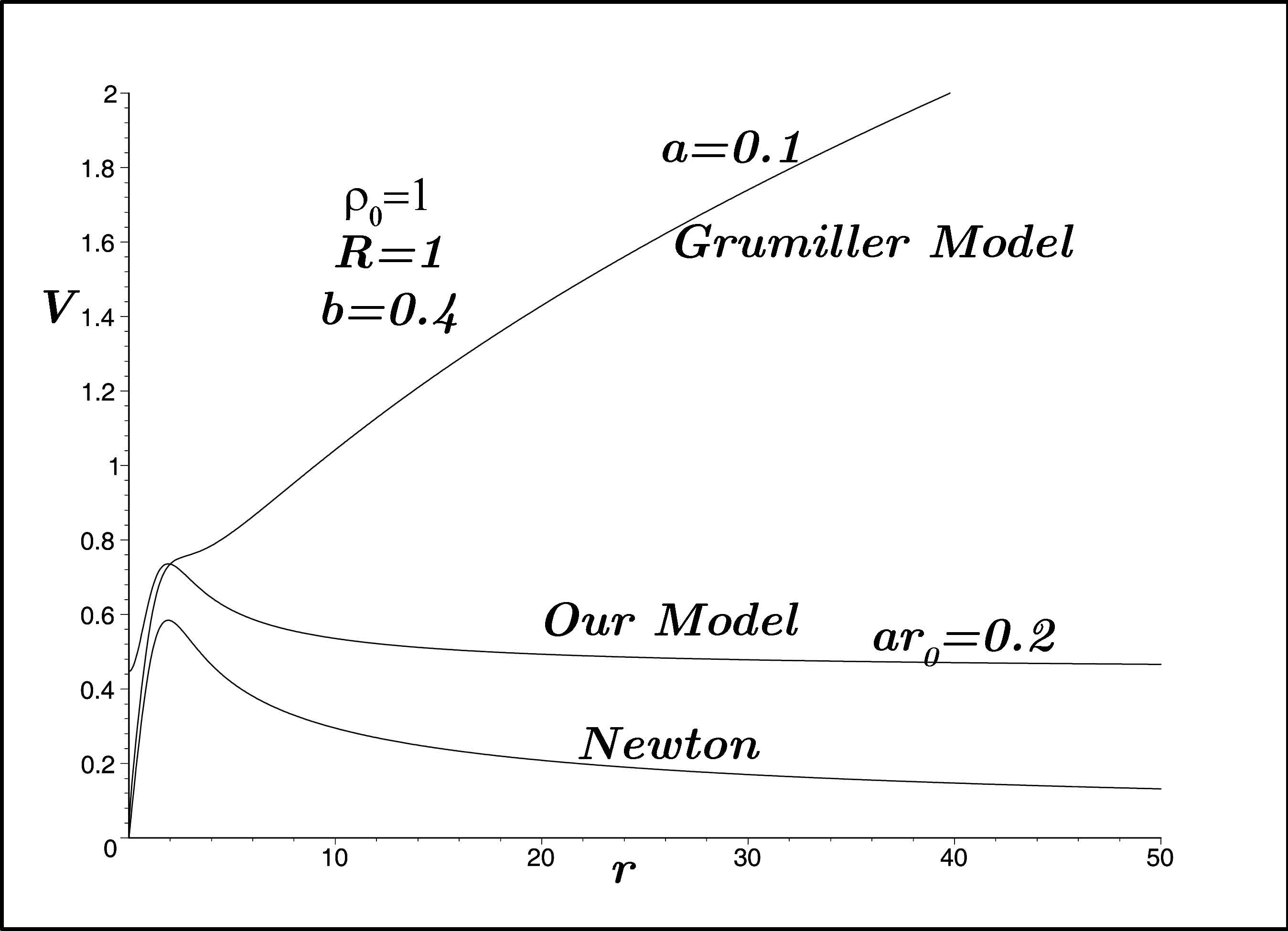
Figure 1: A plot of rotational velocity $v(r)$ versus the radial distance for three different models.

Let’s consider a model for the mass distribution of a galaxy given by

$$\rho=\frac{\rho_{0}}{1+\exp\left(\frac{r-R}{b}\right)}$$ (49)

in which $\rho_{0},$ $R$ and $b$ are real positive constants. The Fig. 1 is a plot of rotational velocity $v(r)$ for three different models.

As a side remark, the problem can be considered from the Newtonian viewpoint. From the Newtonian potential (46) the centripetal force for an object in circular orbit of radius $r$ is given by

$$F_{c}=\frac{m}{r^{2}}+\frac{ar_{0}}{r}$$ (50)

or equivalently

$$F_{c}=\frac{m_{n}}{r^{2}}+\frac{m_{d}}{r^{2}}$$ (51)

in which $m_{n}=m=$ the normal mass and $m_{d}=ar_{0}r=$ the dark mass. We assume a normal matter density $\rho_{n}$ and a dark matter density $\rho_{d}$, such that

$$m_{n}=4\pi\int\nolimits_{0}^{r}\rho_{n}r^{2}dr\text{ and }m_{d}=4\pi\int\nolimits_{0}^{r}\rho_{d}r^{2}dr.$$ (52)

One easily finds $\rho_{d}=\frac{ar_{0}}{4\pi r^{2}}$ while $\rho_{n}$ is given by (49). Now, our aim is to see how the parameters should be adjusted in order to find $\Omega=\frac{m_{d}}{m_{n}}=\frac{23}{4.6}$, i.e. the experimentally recorded ratio. The parameter $\Omega$ is defined by

$$\Omega=\left(\int\nolimits_{0}^{\frac{r_{0}}{\sqrt{e}}}\rho_{d}r^{2}dr\right)/\left(\int\nolimits_{0}^{\frac{r_{0}}{\sqrt{e}}}\rho_{n}r^{2}dr\right)$$ (53)

in which it is assumed that beyond $r_{0}$ both matter and dark matter become insignificant. The latter equation yields

$$\int\nolimits_{0}^{\frac{r_{0}}{\sqrt{e}}}\frac{\rho_{0}}{1+\exp\left(\frac{r-R}{b}\right)}r^{2}dr=\frac{ar_{0}^{2}}{4\pi\sqrt{e}\eta}.$$ (54)

In the zeroth order approximation, one considers a solid central object with a certain boundary at $r=R$ and a uniform mass distribution $\rho_{0}$ which implies ($b\rightarrow 0$)

$$\rho_{0}\left(\frac{R^{3}}{3}\right)=\frac{ar_{0}^{2}}{4\pi\sqrt{e}\xi}.$$ (55)

Herein $a=\frac{\alpha\sqrt{P}}{2\sqrt{2}},$ $r_{0}=\sqrt{P}$ and upon substitution it yields

$$\rho_{0}\left(\frac{R^{3}}{3}\right)=\frac{\alpha P\sqrt{P}}{8\sqrt{2e}\pi\Omega}$$ (56)

which gives the relation between the radius of the central object $R,$ the magnetic charge $P$ and coupling constant $\alpha.$ The normal matter $m_{n}$ will be expressed in terms of charge $\left(P\right)$ and ratio $\Omega$ ($=\frac{23}{4.6}$) by

$$m_{n}=\frac{\alpha P\sqrt{P}}{2\sqrt{2e}\Omega}.$$ (57)

Finally we comment that the effect of dark matter on perihelion precessions has been also considered in 38 .

III CONCLUSION

In conclusion, the idea of nonlinear electrodynamics (NED) popularized in 1930’s by Born and Infeld 39 to resolve singularities remains still attractive and find rooms of applications even in modern cosmology. Specifically, a pure electrical NED model serves to generate Rindler acceleration which was considered responsible for the effects of large distance gravity. A Theorem has been proved to relate the Lagrangian of NED with the metric function. Another (i.e. pure magnetic) NED model modifies the Rindler acceleration term from $\sim 2ar$ to $\sim 2ar_{0}\ln r,$ which yields better flat rotation curves to conform observations. For a detailed analysis of geodesics in the presence of the Rindler term we refer to 40 . As shown (see Fig. 1), our curve lies in between Grumiller (or MK) and Newton models. For this reason without resorting to yet unknown particles dark matter may emerge as a manifestation of NED. The models of NED we employ here have no counterpart in linear, more familiar Maxwell theory. Our models are derived in particular to satisfy the energy (Weak and Strong) conditions and explain the flat rotation curves. As a pay-off in the pure electric case, for instance a global monopole field crops up which lies beyond observation for planets in our solar system. This may be considered much like the cosmological constant, as a background, space-filling uniform electric field to act as the background energy level. Naturally such fields are attributed to topological defects as remnants of big bang which are weak enough to be detected locally. Unfortunately once this field is deleted our energy conditions will be violated. Finally, it will not be wrong to state that NED, which has rarely been appealing may encompass larger scopes in physics / cosmology than envisioned.

III.1 Acknowledgements

We wish to thank the anonymous referee for helpful suggestions. A fruitful correspondence with Prof. D. Grumiller is also appreciated.

References

- (1) N. Arkani-Hamed, S. Dimopoulos and G. R. Dvali, Phys. Lett. B 429, 263 (1998).
- (2) L. Randall and R. Sundrum, Phys. Rev. Lett. 83, 3370 (1999).
- (3) P. D. Mannheim and D. Kazanas, Astrophys. J. 342, 635 (1989).
- (4) P. D. Mannheim, Prog. Part. Nucl. Phys. 56, 340 (2006).
- (5) D. Grumiller, Phys. Rev. Lett. 105, 211303 (2010), 039901(E) (2011).
- (6) S. Carloni, D. Grumiller and F. Preis, Phys. Rev. D 83, 124024 (2011).
- (7) M. Barriola and A. Vilenkin, Phys. Rev. Lett. 63, 341 (1989).
- (8) N. Dadhich, K. Narayan and U. A. Yajnik, Pramana 50, 307 (1998).
- (9) J. Man and H. Cheng, Phys. Rev. D. 87, 044002 (2013).
- (10) J. Sultana and D. Kazanas, Phys. Rev. D 85, 081502(R) (2012).
- (11) S. Habib Mazharimousavi, M. Halilsoy and T. Tahamtan, Eur. Phys. J. C. 72, 1851 (2012).
- (12) N. P. Pitjev and E. V. Pitjeva, Astron. Lett. 39 (2013) 141.
- (13) E. V. Pitjeva and N. P. Pitjev, Mon. Not. Roy. Astron. Soc. 432, 3431 (2013).
- (14) A. Fienga, J. Laskar, P. Kuchynka, H. Manche, G. Desvignes, M. Gastineau, I. Cognard and G. Theureau, Celest. Mech. Dyn. Astr. 111, 363 (2011) .
- (15) E. V. Pitjeva, EPM Ephemerides and Relativity, in Relativity in Fundamental Astronomy, eds. S. A. Klioner, P. K. Seidelmann and M. H. Soffel, Proceedings of the International Astronomical Union, Vol. 261 (Cambridge University Press, Cambridge, 2010), pp. 170-178.
- (16) S. Weinberg, Gravitation and Cosmology: Principles and Applications of the General Theory of Relativity (Wiley, New York, 1972).
- (17) E.V. Pitjeva, Astron. Lett. 31, 340 (2005).
- (18) L. Iorio, Adv. Astron. Astrophys. 2008, 268647 (2008).
- (19) J. D. Anderson et al., Phys. Rev. Lett. 81, 2858 (1998).
- (20) L. Iorio, Int. J. Mod. Phys. D 23, 1450006 (2014).
- (21) L. Iorio, Galaxies vol. 2, no.4, pp. 482-495, 2014.
- (22) L. Iorio, Solar Physics, 281, 815 (2012).
- (23) J. Lense and H. Thirring, Physikalische Zeitschrift 19, 156 (1918). (In German).
- (24) L. Iorio, Int. J. Mod. Phys. D 23, 1450028 (2014).
- (25) L. Iorio, Mon. Not. Roy. Astron. Soc. 437, 3482 (2014).
- (26) T. Damour and G. Schafer, Nuovo Cimento B 101, 127 (1988).
- (27) N. Wex, Class. Quantum Gravity 12, 983 (1995).
- (28) D. P. Whitmire, J. J. Matese, Icarus 165, 219 (2003).
- (29) L. Iorio, JCAP 05, 019 (2011).
- (30) L. Iorio, Mon. Not. Roy. Astron. Soc. 419, 2226 (2012).
- (31) D. Grumiller and F. Preis, Int. J. of Mod. Phys. D 20, 2761 (2011).
- (32) L. Iorio and G. Giudice, New Astronomy, 11, 600 (2006).
- (33) R. H. Sanders, Mon. Not. Roy. Astron. Soc. 370, 1519 (2006).
- (34) M. Sereno and Ph. Jetzer, Mon. Not. Roy. Astron. Soc., 371, 626 (2006).
- (35) G. S. Adkins and J. McDonnell, Phys. Rev. D 75, 082001 (2007).
- (36) J. C. Fabris and J. P. Campos, Gen. Relativ. Gravit. 41:93-104,2009.
- (37) L. Iorio and M. L. Ruggiero, Scholarly Research Exchange, 2008, 968393 (2008).
- (38) L. Iorio, Galaxies, 1, 6 (2013).
- (39) M. Born and L. Infeld, Proc. Roy. Soc. A 144, 425 (1934).
- (40) M. Halilsoy, O. Gurtug and S. H. Mazharimousavi, Gen. Rel. Grav. 45, 2363 (2013).