On three dimensions as the preferred dimensionality of space via the Brandenberger-Vafa mechanism

Brian Greene¹, Daniel Kabat^1,2 and Stefanos Marnerides¹

¹Institute for Strings, Cosmology and Astroparticle Physics

and Department of Physics

Columbia University, New York, NY 10027 USA

²Department of Physics and Astronomy

Lehman College, City University of New York

Bronx, NY 10468 USA

In previous work it was shown that, in accord with the Brandenberger-Vafa mechanism, three is the maximum number of spatial dimensions that can grow large cosmologically from an initial thermal fluctuation. Here we complement that work by considering the possibility of successive fluctuations. Suppose an initial fluctuation causes at least one dimension to grow, and suppose successive fluctuations occur on timescales of order $\alpha^{\prime 1/2}$. If the string coupling is sufficiently large, we show that such fluctuations are likely to push a three-dimensional subspace to large volume where winding modes annihilate. In this setting three is the preferred number of large dimensions. Although encouraging, a more careful study of the dynamics and statistics of fluctuations is needed to assess the likelihood of our assumptions.

1 Introduction

The Brandenberger-Vafa mechanism [1] is one of the few proposals within string cosmology for a mechanism that yields dynamical cosmological growth of three spatial dimensions. The idea that the most basic property of our universe could follow from the dimensionality of fundamental strings is very appealing. For reviews see [2, 3, 4], and for numerical simulations in support of the scenario see [5].

A closer examination of string gas dynamics, however, reveals certain obstacles. To set the stage for the present work, it was found in [6, 7] that – assuming validity of the lowest-order dilaton gravity equations of motion – the dilaton can quickly roll to weak coupling, leaving the universe trapped in the Hagedorn phase. Moreover it was found that – assuming the string gas could be treated as homogeneous – there was no sharp dimension dependence in the string annihilation rate. So given these assumptions, the dynamics did not single out three dimensions as special.

By relaxing the assumption of homogeneity, it was shown in [8] that the mechanism can indeed operate if one takes into account the fact that when winding strings are dilute enough (their mean separation is large compared to their characteristic quantum thickness) they behave semi-classically and their annihilation rates are highly suppressed in more than three large spatial dimensions. The conclusion of [8] was that if the string gas fluctuates out of the Hagedorn regime to a radiation regime in $d$ effective spatial dimensions, then any remaining winding modes are indeed dilute enough that they generically freeze out for $d>3$ and annihilate for $d=3$. Therefore three dimensions is the maximum number of spatial dimensions that can grow large cosmologically due to an initial thermal fluctuation.

In the present work we would like to examine whether three dimensions is also the minimum number of large dimensions that can result from a thermal fluctuation. A priori it seems easier for one or two spatial dimensions to decompactify via the BV mechanism, since it seems more likely that winding modes will find each other in this lower dimensional subspace. If the BV mechanism is indeed the reason the universe has three cosmologically large dimensions, we should address the question of why we don’t observe an effectively lower-dimensional universe.

Answers to this question often turn to anthropic arguments. However in the original proposal of Brandenberger and Vafa, the authors argued that successive thermal fluctuations in the Hagedorn phase would eventually cause the maximum number of dimensions to decompactify. Here we would like to examine this possibility in more detail. We postulate an initial fluctuation that causes one or two dimensions to grow large, and investigate the likelihood of subsequent fluctuations causing a total of three dimensions to decompactify. Thus, in contrast to our previous work [8], we allow for multiple thermal fluctuations. We also relax the assumption of isotropy made in [8]. Besides addressing the question of how many dimensions decompactify, our results will shed light on rapid thermal fluctuations as a possible mechanism for overcoming the obstacle to the BV mechanism pointed out in [6, 7], namely the dilaton rolling to weak coupling.

Essential to our discussion is the fact that, while there might be a window of opportunity for three dimensions to decompactify once one or two dimensions have grown large, there can be no such window for more than three dimensions. That is, anisotropic expansion of one or two dimensions will never favor the eventual decompactification of more than three dimensions. To see this, consider the case of $d>3$ isotropic large dimensions, where the equilibrium state is radiation in $d$ dimensions and the winding modes want to annihilate. The annihilation rate of these winding modes depends on the size $R$ of the large dimensions in two ways [8]. First, there is an enhancement $\sim R^{2}$ reflecting the fact that longer strings are more likely to annihilate. Second, with $\Delta x\sim\sqrt{\log R}$ the characteristic quantum thickness of a string of length $R$, the amplitude has an impact parameter suppression $\sim\exp(-({b}/{\Delta x})^{2})$ in the $d-3$ large directions transverse to string collisions. This exponential suppression was put forward in [8] as essential to the BV mechanism, in the sense that winding modes will freeze out if $d>3$. Now imagine we let some of these dimensions shrink while others grow. We do this to effect anisotropy, however we preserve the total volume (and energy) so the equilibrium state does not change. This will only further (and exponentially) suppress the annihilation of winding modes around the smaller dimensions, by increasing the impact parameters in the larger dimensions. So strings winding the smaller dimensions are even less likely to annihilate than in the isotropic case studied in [8]. Since the isotropic case already singled out $d\leq 3$, we conclude that only $d\leq 3$ dimensions can decompactify as a result of anisotropic fluctuations.

Hence studying anisotropic fluctuations within a three-dimensional subspace accommodates the relevant cases for decompactification. Given an initial thermal fluctuation that causes some number of dimensions to grow, our goal is to study the likelihood of subsequent fluctuations causing three dimensions to decompactify. To keep the investigation tractable we will only consider one degree of anisotropy, namely between one large and two small dimensions, or between one small and two large dimensions.

An outline of this paper is as follows. In section 2 we set up the dynamical equations and discuss the possible equilibrium phases of the system. In section 3 we give our procedure for choosing initial conditions and sampling thermal fluctuations. In section 4 we present our numerical results, and in section 5 we discuss their implications for the Brandenberger-Vafa mechanism.

2 Dynamics

The general setup will follow the lines of [8], which the reader may refer to for more details. The difference is that here we are considering two (logarithmic) scale factors, $\nu$ and $\lambda$, respectively for the $d_{1}<3$ dimensions initially unwound and growing, and for the $d_{2}=3-d_{1}$ dimensions subsequently expanding after a fluctuation, but wrapped with winding modes.

We work in type IIA string theory, on a flat toroidal background with metric (in $\alpha^{\prime}=1$ units)

$$ds^{2}=-dt^{2}+e^{2\nu(t)}\sum_{i=1}^{d_{1}}dx_{i}^{2}+e^{2\lambda(t)}\sum_{i=d_{1}+1}^{3}dx_{i}^{2}\hskip 22.76219pt0\leq x_{i}\leq 2\pi$$ (1)

All other dimensions are held fixed at the self-dual radius. We also have the homogeneous shifted dilaton field $\varphi(t)=2\phi(t)-d_{1}\nu(t)-d_{2}\lambda(t)$. When the metric and dilaton are coupled to matter, the equations of motion are

$$\ddot{\varphi} =\frac{1}{2}(\dot{\varphi}^{2}+d_{1}\dot{\nu}^{2}+d_{2}\dot{\lambda}^{2})$$ (2)

$$\ddot{\nu} =\dot{\varphi}\dot{\nu}+\frac{1}{8\pi^{2}}e^{\varphi}P_{\nu}$$

$$\ddot{\lambda} =\dot{\varphi}\dot{\lambda}+\frac{1}{8\pi^{2}}e^{\varphi}P_{\lambda}$$

Here $P_{\nu},\,P_{\lambda}$ are the pressures along the $d_{1},\,d_{2}$ dimensions respectively. Note that we do not consider a potential for the dilaton. There is also the Hamiltonian constraint (or Friedmann equation)

$$E=(2\pi)^{2}e^{-\varphi}(\dot{\varphi}^{2}-d_{1}\dot{\nu}^{2}-d_{2}\dot{\lambda}^{2})$$ (3)

where $E$ is the total energy in matter. We take matter to consist of

• Winding modes, with $W$ denoting the winding number of strings wound with positive orientation. For simplicity we assume this winding number is carried by $W$ individual strings, each having a single unit of positive winding. This is a conservative assumption, since taking multiply-wound strings into account would lead to a larger annihilation rate. Also note that since we are working in a compact space, the net winding number must vanish, which means there are an equal number of strings wound with the opposite orientation. Since the $d_{1}$ dimensions are assumed unwound to begin with, the winding modes only wrap the dimensions $d_{2}$. These winding modes evolve according to

  $$\dot{W}=-\Gamma_{W}(W^{2}-\langle W\rangle^{2})$$ (4)

  Here $\langle W\rangle$ denotes the equilibrium average winding and $\Gamma_{W}$ is an interaction rate we specify below. The contribution to the energy from winding and anti-winding modes is $E=2d_{2}We^{\lambda}$ and their contribution to the (off-equilibrium) pressure is $P_{\lambda}=-2We^{\lambda}$.

• Radiation, or pure Kaluza-Klein modes, with $K_{\nu}$ and $K_{\lambda}$ denoting the momentum numbers of strings with positive momentum along the $d_{1}$ and $d_{2}$ dimensions respectively. We assume this momentum is carried by individual strings that each have one unit of positive Kaluza-Klein momentum; the net momentum vanishes so there must be an equal number of strings with negative momentum. These momentum modes evolve according to

  $$\dot{K}_{\nu} =-\Gamma_{K_{\nu}}(K_{\nu}^{2}-\langle K_{\nu}\rangle^{2})$$ (5)

  $$\dot{K}_{\lambda} =-\Gamma_{K_{\lambda}}(K_{\lambda}^{2}-\langle K_{\lambda}\rangle^{2})$$

  The energy in these modes is $E=2d_{1}K_{\nu}e^{-\nu}+2d_{2}K_{\lambda}e^{-\lambda}$ and their contributions to the pressures are $P_{\nu}=2K_{\nu}e^{-\nu}$, $P_{\lambda}=2K_{\lambda}e^{-\lambda}$.

• String oscillator modes which we model as pressureless matter.

2.1 Equilibrium phases

In this section we review the possible equilibrium phases of a string gas. This information will be important in the sequel, when we study fluctuations and the approach to equilibrium. A point of terminology: in the remainder of this paper, when we refer to the universe as being in one of these possible phases, we do not mean that the universe is actually in thermal equilibrium. Rather we are using these names as a convenient shorthand to indicate what the equilibrium state of the universe would be, given its energy density.

In the $d$-dimensional isotropic case the string gas has two possible equilibrium thermodynamic phases. In the Hagedorn phase massive and massless modes are in thermal equilibrium, the pressure vanishes and the energy in matter is conserved. At lower energy densities the equilibrium state of the universe is radiation dominated. This occurs when the energy density in $d$ dimensions satisfies

$$\rho_{d}=\frac{E}{V_{d}}<\rho_{H}=c_{d}T_{H}^{d+1}$$ (6)

with $T_{H}$ the Hagedorn temperature and $c_{d}$ the Stefan-Boltzmann constant in $d$ dimensions. This can be alternatively expressed in terms of temperatures. In a volume $V_{d}$ with energy $E$, a radiation gas has temperature $T_{d}=(\frac{E}{c_{d}V_{d}})^{\frac{1}{d+1}}$. The condition (6) can be then expressed as

$$T_{d}<T_{H}$$ (7)

That is, the universe is radiation-dominated when the would-be radiation temperature falls below the Hagedorn temperature.

In the anisotropic case there is an additional possibility. Recall that we have three large dimensions, with $d_{1}$ of them larger than the remaining $d_{2}=3-d_{1}$. Besides the Hagedorn phase, the system could be found in either a 3-dimensional or a $d_{1}$-dimensional radiation phase. To fix the equilibrium phase of the universe we generalize the condition (7). Given the energy of the system and the 3-dimensional and $d_{1}$-dimensional volumes, the lower of the two temperatures $T_{d_{1}}=(\frac{E}{c_{d_{1}}V_{d_{1}}})^{\frac{1}{d_{1}+1}}$ and $T_{3}=(\frac{E}{c_{3}V_{3}})^{\frac{1}{4}}$ determines the equilibrium phase. If neither of these temperatures is lower than $T_{H}$ then the system is in the Hagedorn phase. For brevity, we will refer to these equilibrium phases as $\mathcal{R}_{d_{1}}$, $\mathcal{R}_{3}$ and $\mathcal{H}$.

In equilibrium in $\mathcal{R}_{d_{1}}$ the energy is entirely carried by the massless Kaluza-Klein modes $K_{\nu}$. Treating these modes as a collection of one-dimensional gasses, the equilibrium values are [6]

$$\mathcal{R}_{d_{1}}:\hskip 8.53581pt\begin{aligned} &\langle K_{\nu}\rangle=\frac{E}{2d_{1}}e^{\nu},\\ &\langle K_{\lambda}\rangle=\langle W\rangle=0\end{aligned}$$ (8)

These values account for all of the available energy, see below (5). They correspond to pressures

$$\mathcal{R}_{d_{1}}:\hskip 8.53581pt\langle P_{\nu}\rangle=\frac{E}{d_{1}},\hskip 5.69054pt\langle P_{\lambda}\rangle=0$$ (9)

In equilibrium in $\mathcal{R}_{3}$ the energy is split between $K_{\nu}$ and $K_{\lambda}$, $E=2d_{1}K_{\nu}e^{-\nu}+2d_{2}K_{\lambda}e^{-\lambda}$. Recalling that $d=3=d_{1}+d_{2}$ the equilibrium values are

$$\mathcal{R}_{3}:\hskip 8.53581pt\begin{aligned} &\langle K_{\nu}\rangle=\frac{E}{6}e^{\nu},\\ &\langle K_{\lambda}\rangle=\frac{E}{6}e^{\lambda},\hskip 5.69054pt\langle W\rangle=0\end{aligned}$$ (10)

corresponding to pressures

$$\mathcal{R}_{3}:\hskip 8.53581pt\langle P_{\nu}\rangle=\langle P_{\lambda}\rangle=\frac{E}{3}$$ (11)

Finally in the Hagedorn phase the equilibrium values are [6]

$$\mathcal{H}:\hskip 8.53581pt\begin{aligned} &\langle K_{\nu}\rangle=\frac{1}{12}\sqrt{\frac{E}{\pi}}e^{\nu},\\ &\langle K_{\lambda}\rangle=\frac{1}{12}\sqrt{\frac{E}{\pi}}e^{\lambda},\hskip 5.69054pt\langle W\rangle=\frac{1}{12}\sqrt{\frac{E}{\pi}}e^{-\lambda}\end{aligned}$$ (12)

with pressures (due to the lack of winding around $d_{1}$)

$$\mathcal{H}:\hskip 8.53581pt\langle P_{\nu}\rangle=\frac{1}{6}\sqrt{\frac{E}{\pi}},\hskip 5.69054pt\langle P_{\lambda}\rangle=0$$ (13)

We also recall the off-equilibrium interaction rates [6]. In the radiation phases, for strings with a single unit of momentum or winding, the rates are

$$\Gamma_{K_{\nu}}=\frac{1}{\pi}e^{-2\nu+\varphi},\hskip 8.53581pt\Gamma_{K_{\lambda}}=\frac{1}{\pi}e^{-2\lambda+\varphi},\hskip 8.53581pt\Gamma_{W}=\frac{1}{\pi}e^{2\lambda+\varphi}.$$ (14)

In the Hagedorn phase these rates get multiplied by a factor $16\pi E/9$ reflecting the enhancement due to highly excited oscillator modes.

3 Fluctuations, initial conditions and procedure

We are interested in the likelihood of decompactifying three dimensions as a result of successive fluctuations. To this end we consider the following scenario. The first fluctuation occurs at time $t=0$ and takes the universe to a state in which $d_{1}<3$ dimensions are expanding and free from winding. The initial size of these dimensions is $\nu_{0}>0$ and their initial expansion rate is $\dot{\nu}_{0}>0$. For simplicity we treat all other dimensions as fixed in size, with vanishing expansion rates. Then at time $t_{f}$ some number of dimensions $d_{2}=3-d_{1}$ fluctuate to a size $\lambda(t_{f})$ and begin expanding at a rate $\dot{\lambda}(t_{f})>0$. We assume that $0<\lambda(t_{f})<\nu(t_{f})$. This models an energy fluctuation with energy flowing from matter to gravitation. We are interested in the likelihood that all three dimensions will decompactify, that is, that the winding modes wrapping the $d_{2}$ dimensions will annihilate and that all three dimensions will begin to expand. We will study this as a function of the initial conditions, the fluctuation time $t_{f}$ and the anisotropy parameter

$$r\equiv\frac{R_{\lambda}}{R_{\nu}}(t_{f})=e^{\lambda(t_{f})-\nu(t_{f})}$$ (15)

Depending on the energy density, the universe could start out at $t=0$ with any one of the three possible equilibrium phases $\mathcal{R}_{3}$, $\mathcal{R}_{d_{1}}$, or $\mathcal{H}$. If the universe starts with $\mathcal{R}_{3}$ as its equilibrium phase then there is no need for a subsequent fluctuation: there will be few or no winding strings present – from (10) we have $\langle W\rangle=0$ – so the initial conditions will most likely directly lead to three-dimensional decompactification. Another possibility is that at time $t=0$ the universe could start with $\mathcal{R}_{d_{1}}$ as its equilibrium phase. In this case it is quite possible that the strings winding around the $d_{2}$ dimensions will eventually annihilate. This would allow the universe to relax to equilibrium in the phase $\mathcal{R}_{d_{1}}$. But from (8), (9) note that in equilibrium in $\mathcal{R}_{d_{1}}$ we have $\langle K_{\lambda}\rangle=\langle W\rangle=0$, which means the pressure in the $d_{2}$ dimensions vanishes. So even though the $d_{2}$ dimensions can shed their winding, it seems unlikely that these dimensions will begin to expand. Instead we expect them to remain small and unwound. This leads us to make a conservative assumption, that if the universe finds itself with $\mathcal{R}_{d_{1}}$ as its equilibrium phase it will never become effectively three dimensional. This assumption could be lifted through a more careful study of fluctuations, which might show some probability of decompactification even starting from $\mathcal{R}_{d_{1}}$. As we do not attempt such a study here, we employ the conservative assumption that a universe which begins in $\mathcal{R}_{d_{1}}$ will never end up with three large dimensions.

Thus in order to obtain three large dimensions from successive fluctuations, at time $t=0$ the system should find itself with $\mathcal{H}$ as its equilibrium phase. Given $\nu_{0}$, this puts a lower bound on the energy at $t=0$,

$$E\geq c_{d_{1}}V_{d_{1}}T_{H}^{d_{1}+1}$$ (16)

At fixed volume, this essentially constrains the initial value of the dilaton as we will see shortly.

One might worry that starting in $\mathcal{H}$ at $t=0$ leads to a further restriction when we require that the $d_{1}$ dimensions are initially unwound. The issue is that in the Hagedorn phase the equilibrium winding number does not vanish, unless the ratio $E/e^{\nu}$ is small enough that no winding is energetically allowed. In practice this is not a concern. As we will see below, in order for the eventual decompactification of three dimensions to take place, the initial value of $\nu_{0}$ must be large enough, and the initial energy low enough, that initial conditions which allow decompactification of three dimensions are consistent with the condition that the $d_{1}$ dimensions start out unwound. Another way to see this is to assume the contrary as follows. Suppose we start deep in the Hagedorn phase where the $d_{1}$ dimensions are wound. Then when the $d_{2}$ dimensions fluctuate, it is unlikely that they will be able to push the system out of $\mathcal{H}$ and into $\mathcal{R}_{3}$. Thus if the $d_{1}$ dimensions start out wound, fluctuations can occur but will most likely just leave the universe trapped in the Hagedorn phase.

At this point we review our procedure for fixing initial conditions. The maximum value of $|\dot{\varphi}|$ consistent with the supergravity approximation is $|\dot{\varphi}|=1$. Orienting time so the universe is rolling to weak coupling, we set $\dot{\varphi}_{0}=-1$. This defines our initial time slice; the equations of motion then guarantee that $|\dot{\varphi}(t)|<1$ and $\dot{\varphi}(t)<0$ for all $t$. To explore the dependence on $\varphi_{0}$ we will scan over a range of values specified below, consistent with the universe starting in the Hagedorn phase. Given $\dot{\varphi}_{0}$ and $\varphi_{0}$, the expansion rate $\dot{\nu}_{0}$ is chosen at random. The total energy in the universe vanishes by the Hamiltonian constraint, so we assume the relevant probability distribution for $\dot{\nu}_{0}$ is given by the microcanonical ensemble. This distribution turns out to have a Gaussian form. To see this note that

$$\text{prob}(\dot{\nu}_{0})\sim\text{exp}(S)=\text{exp}(E/T_{H})\propto\text{exp}\bigl{[}-\bigl{(}\frac{4\pi^{2}d_{1}e^{-\varphi_{0}}}{T_{H}}\bigr{)}\dot{\nu_{0}}^{2}\bigr{]}$$ (17)

where we used the Hagedorn equation of state to determine the entropy, $S=E/T_{H}$, and we used the Hamiltonian constraint (3) to determine the energy available in matter. Finally we make a choice for $\nu_{0}$, which controls the size of the dimensions $d_{1}$. In practice we will test two values, $\nu_{0}=3$ and $\nu_{0}=5$. Note that via the constraint (3), the quantities $\dot{\varphi}_{0}$, $\varphi_{0}$, $\dot{\nu}_{0}$ are sufficient to determine the energy in matter at $t=0$. Given the energy in matter and a choice for $\nu_{0}$, the initial Kaluza-Klein momentum in the large dimensions $K_{\nu}(t=0)$ is set to its equilibrium value.

We then evolve the system to time $t_{f}$ using the equations of motion (2), (4), (5). During this time we hold $\lambda=0$ fixed at the self-dual radius. At time $t_{f}$ we effect a fluctuation for the dimensions $d_{2}$. To model a fluctuation we draw energy from the bath of heavy oscillator modes and re-distribute that energy to the other matter and metric modes, i.e. to the expansion rates. We specify the size of the fluctuation, that is the value of $\lambda(t_{f})$, using the anisotropy parameter $r$ defined in (15). In practice we will scan over the range $0.1<r<1$. Then using $\dot{\varphi}(t_{f})$, $\varphi(t_{f})$ and $\dot{\nu}(t_{f})$ we evaluate the energy in matter for $\dot{\lambda}=0$ and tentatively determine the equilibrium phase of the universe. This allows us to choose the expansion rate $\dot{\lambda}(t_{f})$ from a Gaussian probability distribution, where the width of the Gaussian is determined as follows. In the Hagedorn phase we have a result similar to (17),

$$\text{prob}(\dot{\lambda})\sim\text{exp}(S)=\text{exp}(E/T_{H})\propto\text{exp}\bigl{[}-\bigl{(}\frac{4\pi^{2}d_{2}e^{-\varphi}}{T_{H}}\bigr{)}\dot{\lambda}^{2}\bigr{]}$$ (18)

and we read off the variance

$$\sigma_{\mathcal{H}}^{2}=\frac{T_{H}e^{\varphi}}{8\pi^{2}d_{2}}$$ (19)

In the radiation phase $\mathcal{R}_{3}$, on the other hand, the matter entropy is

$$S={d+1\over d}c_{d}V_{d}T^{d}={d+1\over d}(c_{d}V_{d})^{1\over d+1}E^{d\over d+1}$$ (20)

Using (3) to determine the available energy and expanding in powers of $\dot{\lambda}$ we have

$$\text{prob}(\dot{\lambda})\sim\text{exp}(S)\propto\text{exp}\bigl{[}-\dot{\lambda}^{2}/2\sigma_{\mathcal{R}_{3}}^{2}\bigr{]}$$ (21)

where the variance is

$$\sigma_{\mathcal{R}_{3}}^{2}={1\over 2d_{2}}\left({\dot{\varphi}^{2}\over c_{d}V_{d}}\right)^{1\over d+1}\left({e^{\varphi}\over 4\pi^{2}}\right)^{d\over d+1}$$ (22)

Once $\dot{\lambda}(t_{f})$ is chosen we re-calculate the energy available to matter. We still need to determine the values of $K_{\lambda}(t_{f})$ and $W(t_{f})$. These are chosen from a uniform distribution. We randomly select $K_{\lambda}(t_{f})$ in the range $(K_{\text{self-dual}},K_{\text{equilibrium}})$ and $W(t_{f})$ in the range $(\text{Max}\{0.5,\langle W\rangle\},W_{\text{self-dual}})$. Note that the values at the self-dual radius ($\lambda=0$) set a lower bound on $K_{\lambda}$ and an upper bound on $W$. Also the value $0.5$ is our cutoff value for rounding down to no winding: we do not allow the fluctuation to result in vanishing winding, as our goal is to test whether the winding modes will annihilate as a consequence of interactions.

In summary, the values $\varphi_{0}$, $\dot{\varphi}_{0}$, $\nu_{0}$, $K_{\nu}(t=0)$ and $\lambda(t_{f})$ (or $r$) are fixed and we randomly choose $\dot{\nu}_{0}$, $\dot{\lambda}(t_{f})$, $K_{\lambda}(t_{f})$ and $W(t_{f})$ from the distributions given above. For $t>t_{f}$ we solve the equations of motion until the winding modes either freeze out or annihilate completely. In practice, when we numerically integrate the equations of motion, the winding modes are considered annihilated when $W<0.5$ and frozen when $\Gamma_{W}W<0.1\dot{\nu}$. (This is the relevant comparison of interaction rate and expansion rate, appropriate for the Boltzmann equation (4). The use of $\dot{\nu}$ here reflects the fact that the winding modes collide in the $d_{1}$ dimensions.) This lies at the heart of our test of the BV mechanism: the dimensions $d_{1}$ are unwound and free to expand, and we test whether the winding modes wrapping the remaining $d_{2}$ dimensions can stay in equilibrium as they compete with the expansion rate $\dot{\nu}$ of the $d_{1}$ larger dimensions.

A note is in order regarding fluctuations of the scale factors. Given the Hagedorn equation of state $S=E/T_{H}$ we assume the scale factors can fluctuate randomly with a uniform distribution, since there is no cost in entropy. This is true in the thermodynamic limit. However, the (equilibrium) entropy receives corrections at large radii, given by [10, 11]

$$\Delta S=\text{log}\left[1-\sum_{i}\Gamma(2d_{i})^{-1}(\eta_{i}E)^{2d_{i}-1}e^{-\eta_{i}E}\right],\hskip 14.22636pt\eta_{i}=T_{H}^{-1}\left(1-\sqrt{1-\frac{1}{2R_{i}^{2}}}\,\right)$$ (23)

for each set of $d_{i}$ dimensions with radius $R_{i}$. These corrections are negligible when compared to the leading term, typically by many orders of magnitude. The probability distribution resulting from this correction as a function of $R$ at constant matter energy is very flat in the Hagedorn phase. There is a mild dip around $\eta_{i}E=2d_{i}-1$, but this lies outside the Hagedorn phase except when $d_{i}=1$. We ignore these corrections and adopt a flat distribution for scale factor fluctuations.

4 Results

For the scale factor $\nu_{0}$ associated with the initial size of the universe we consider two possible values, $\nu_{0}=3$ and $\nu_{0}=5$. We will see that the results only mildly depend on the choice of $\nu_{0}$. As values of $\nu_{0}$ larger than $5$ are in a sense “too large,” since they correspond to radii far larger than the string scale, we trust that these two values provide a good test of the Brandenberger-Vafa mechanism.

Once $\nu_{0}$ is chosen, the condition (16) that the system starts in $\mathcal{H}$ at $t=0$ translates to the following condition on the value of $\varphi_{0}$:

$$\varphi_{0}\lesssim-d_{1}\nu_{0}-\log[(2\pi)^{d_{1}-2}c_{d_{1}}T_{H}^{d_{1}+1}]$$ (24)

(We’re using the fact that $\dot{\varphi}_{0}=-1$, while the Hubble rates in (3) are much smaller than 1). The above is not a severe constraint since it is consistent with the prerequisite of weak coupling, although it constrains the case $d_{1}=2$ more than $d_{1}=1$ since it pushes us to weaker values for the coupling. The condition that the $d_{1}$ dimensions start out unwound, $\langle W\rangle<0.5$, translates to

$$\varphi_{0}\gtrsim-2\nu_{0}-\log[9/\pi]$$ (25)

Taken together, (24) and (25) fix the range of dilaton values we want to test. What happens outside this range? At stronger values of the coupling, corresponding to less initial energy, the system is found in $\mathcal{R}_{d_{1}}$ at $t=0$. As discussed in the paragraph below (15), we make the conservative assumption that in this case additional dimensions will never decompactify, even if they shed their winding. On the other hand at weaker values of the coupling the system is trapped forever in the Hagedorn phase, with all dimensions wound.

For the fluctuation time $t_{f}$ we consider three possible values, $t_{f}=1$, $10$, $100$ in string units ($\alpha^{\prime}=1$). This turns out to be the most decisive parameter, with $t_{f}=1$ giving the largest window for decompactification of three dimensions.

To summarize the initial conditions, we fix $\nu_{0}\in\{3,5\}$ and $t_{f}\in\{1,10,100\}$. We then scan over $0<r<1$ and the range of $\varphi_{0}$ dictated by (24) and (25). For each choice of initial conditions we perform 100 integrations of the equations of motion to sample values of $\dot{\nu}_{0}$, $\dot{\lambda}(t_{f})$, $K_{\lambda}(t_{f})$ and $W(t_{f})$ from the distributions mentioned above.

Our results are shown in Figs. 1 and 2, where we plot the number of cases for which the winding modes annihilate as a function of $\varphi_{0}$ and $r$. The dependence on $\varphi_{0}$ and $r$ is as expected, with strong coupling (large $\varphi_{0}$) and large fluctuations (large $r$) more likely to decompactify. The dependence on $\nu_{0}$ is rather mild. The constraints (24), (25) push us to weaker coupling as $\nu_{0}$ is increased, but the enhancement in the annihilation amplitude $\sim e^{2\lambda(t_{f})}=r^{2}e^{2\nu(t_{f})}$ makes up for this suppression. A striking feature is the dependence of the plots on $t_{f}$. The reason decompactification becomes unlikely at large $t_{f}$ is the rolling of the dilaton to weak coupling. This suppresses the rates (14) and makes it impossible for wound strings to annihilate. Note that this leads to a degeneracy, that a large value for $t_{f}$ can be compensated by starting with a stronger coupling or a smaller value of $\dot{\varphi}$.

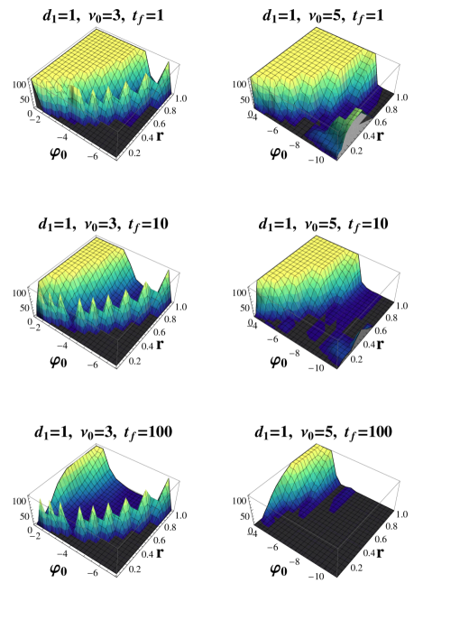
Figure 1: Number of cases decompactifying (out of 100) as a function of $\varphi_{0}$ and $r$, for $\nu_{0}=3,5$ and $t_{f}=1,10,100$ when $d_{1}=1$.

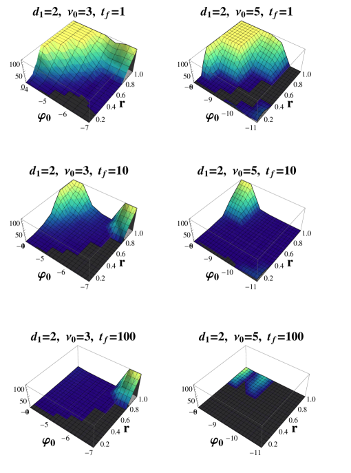
Figure 2: Number of cases decompactifying (out of 100) as a function of $\varphi_{0}$ and $r$, for $\nu_{0}=3,5$ and $t_{f}=1,10,100$ when $d_{1}=2$.

In all cases, the decisive factor for decompactification is the energy density of the universe. This is shown in Figs. 3 and 4. On these graphs we show contour plots for the number of cases decompactifying. We also show the contour (thick black line) corresponding to the energy density that separates an equilibrium phase $\mathcal{H}$ from an equilibrium phase $\mathcal{R}_{3}$. We also show the contour (thin red line) for the energy density below which more than $90\%$ of the cases result in three dimensions decompactifying.

The main lesson is that a fluctuation is quite likely to make three dimensions decompactify provided the fluctuation is large enough to push the equilibrium phase of the universe well into $\mathcal{R}_{3}$. As in [8], a small fluctuation may leave the universe trapped in $\mathcal{H}$, although what we mean by this here is that the winding modes freeze out while the $d_{1}$ dimensions keep growing. Note that there is a narrow region – near the critical energy density separating $\mathcal{H}$ and $\mathcal{R}_{3}$ – where it is possible that $\langle W\rangle$ is non-zero after the fluctuation, but drops to zero as the universe expands. If this happens while interactions are still efficient the winding modes will annihilate. This is responsible for the spiky ridge seen in Fig. 1. This discussion also makes it clear that the contours of constant decompactification probability track the contours of constant energy density. To understand this, note that energy density is the key parameter which determines whether the universe has Hagedorn or radiation as its equilibrium phase.

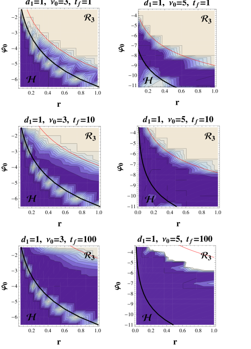
Figure 3: Contours of constant probability of decompactification for $d_{1}=1$. The thick black line is the energy density separating the equilibrium radiation and equilibrium Hagedorn phases. The thin red line is the energy density below which more than $90\%$ of the cases decompactify.

Figure 4: Same as Figure 3 but for $d_{1}=2$.

Since energy density is the most important parameter, in Table 1 we give the range of energy densities at time $t_{f}$ that lead to three dimensions decompactifying. We also express our results as a function of $d_{1}$, $\nu_{0}$ and $t_{f}$ by giving the percentage of cases that decompactify three dimensions in Table 2.

$d_{1}=1$
	$t_{f}=1$	$t_{f}=10$	$t_{f}=100$
$\nu_{0}=3$	$(1.5\sim 65)\times 10^{-9}$	$(1.5\sim 15)\times 10^{-9}$	$(1.5\sim 2.8)\times 10^{-9}$
$\nu_{0}=5$	$(2.4\sim 640)\times 10^{-11}$	$(2.4\sim 195)\times 10^{-11}$	$(2.4\sim 7.1)\times 10^{-11}$
$d_{1}=2$
	$t_{f}=1$	$t_{f}=10$	$t_{f}=100$
$\nu_{0}=3$	$(1.4\sim 6.5)\times 10^{-8}$	$(1.4\sim 3.1)\times 10^{-8}$	$0$
$\nu_{0}=5$	$(2.3\sim 10)\times 10^{-9}$	$(2.3\sim 3.9)\times 10^{-9}$	$0$

Table 1: The range of energy densities at time $t_{f}$ that lead to three dimensional decompactification.

$d_{1}=1$
	$t_{f}=1$	$t_{f}=10$	$t_{f}=100$
$\nu_{0}=3$	$82$	$53$	$20$
$\nu_{0}=5$	$65$	$47$	$17$
$d_{1}=2$
	$t_{f}=1$	$t_{f}=10$	$t_{f}=100$
$\nu_{0}=3$	$70$	$26$	$1$
$\nu_{0}=5$	$43$	$13$	$0.1$

Table 2: Percentage of cases yielding three-dimensional decompactification, showing the dependence on $d_{1}$, $\nu_{0}$, $t_{f}$.

5 Discussion

In this paper we studied a model in which successive thermal fluctuations are able to decompactify a total of three dimensions. Although these dimensions are initially anisotropic, it was argued in [9] that string gas cosmology will eventually lead to isotropization. So roughly speaking our results support the BV mechanism, as providing a candidate stringy origin of the universe we observe. However a more refined statement is that in our model the probability of decompactifying three dimensions depends on several parameters, in particular on the fluctuation time $t_{f}$ and the energy density $E(t_{f})$. We now discuss the implications of these results for the BV mechanism.

We found that three large dimensions can arise provided scale factor fluctuations in the Hagedorn phase occur frequently, on a timescale $t_{f}\sim\sqrt{\alpha^{\prime}}$. These frequent fluctuations are necessary so that the dilaton does not have time to roll to weak coupling. It seems reasonable to take $t_{f}\sim\sqrt{\alpha^{\prime}}$, since $\sqrt{\alpha^{\prime}}$ is the natural timescale of the system in the Hagedorn phase.

Assuming $t_{f}\sim\sqrt{\alpha^{\prime}}$, the energy density $E(t_{f})$ is basically fixed by the initial value of the dilaton. To address the dependence on this quantity consider two successive fluctuations, the first at time $t=0$, the second at time $t\sim\sqrt{\alpha^{\prime}}$. The initial value of the dilaton $\varphi_{0}$ determines the subsequent possibilities. First, there is a relatively narrow range towards strong coupling where the equilibrium phase at $t=0$ is $\mathcal{R}_{d_{1}}$. In this case we do not expect additional dimensions to decompactify. So other than invoking anthropic arguments, we see no way to argue for a three-dimensional outcome. But if the initial coupling is not too strong, then we start in $\mathcal{H}$ and the following possibilities remain. One possible outcome, which fortunately occupies the smallest volume in the space of initial conditions, is that the system lands in the part of $\mathcal{R}_{3}$ where the winding modes wrapping the $d_{2}$ smaller dimensions cannot annihilate. In that case, we again expect only $d_{1}$ dimensions to grow large. But for most initial conditions the universe either ends up in the part of $\mathcal{R}_{3}$ where a total of three dimensions decompactify, or remains stuck in the Hagedorn phase.

This latter possibility, of staying in the Hagedorn phase, may seem discouraging. But in fact it could work in favor of the BV mechanism, because roughly speaking it brings us back to square one. As time goes by the scale factors may evolve slightly, but if fluctuations occur frequently enough this evolution is inconsequential. The key point is that even if the $d_{1}$ dimensions are unwound and experience positive pressure, when the system is in equilibrium in $\mathcal{H}$ their growth over many string times is tiny. This is because the energy in radiation ($\sim\sqrt{E}$) is much smaller than the energy in matter ($\sim E$), and furthermore the matter energy is very nearly independent of $\nu$. This nearly constant large energy keeps the velocity of the dilaton large, but also results in large “dilaton friction” and a negligible change in $\nu$. This can be seen by writing the equations of motion in the form

$$\frac{d}{dt}(e^{-\varphi}\dot{\varphi}) =-\frac{1}{8\pi^{2}}E$$ (26)

$$\frac{d}{dt}(e^{-\varphi}\dot{\nu}) =\frac{1}{48\pi^{2}\sqrt{\pi}}\sqrt{E}$$

In our numerical solutions, even for $t_{f}=100$, the most that $\nu$ changed was by one part in a hundred, while the energy remained constant to one part in a few thousand. Thus the $d_{1}$ dimensions can “hover” in the Hagedorn phase for a long time, which allows additional fluctuations to take place. Of course during this time the dilaton is rolling monotonically towards weak coupling [6, 7], so if too much time goes by before another fluctuation takes place, the string coupling will become so small that the winding modes are unable to annihilate. But with a fluctuation timescale $t_{f}\sim\sqrt{\alpha^{\prime}}$, this may not be a significant concern. To summarize, within our model we find that there is a considerable window in which scale factor fluctuations favor the eventual decompactification of three dimensions, provided such fluctuations occur on timescales $\sim\sqrt{\alpha^{\prime}}$.

We conclude with a few issues which must be addressed in order to reach a definitive conclusion regarding the robustness of the BV mechanism.

• We found that the BV mechanism can operate provided there are fluctuations into a regime where winding strings are dilute. This raises the crucial issue of whether a dilute string gas in the early universe can evolve towards a homogeneous cosmology at late times. Studying this requires going beyond our mini-superspace approximation, in which we only kept the homogeneous modes of the metric and dilaton.

• We found that the BV mechanism can operate provided fluctuations in the scale factors occur on timescales of order $\sqrt{\alpha^{\prime}}$. It seems reasonable to assume $t_{f}\sim\sqrt{\alpha^{\prime}}$ in the Hagedorn phase. But this assumption should be validated, for example by deriving the statistics of fluctuations from a study of the stochastic evolution of scale factors coupled to a hot string gas.

Acknowledgements

The work of DK was supported in part by NSF grants PHY-0855582 and PHY-1214410 and by PSC-CUNY grants.

References

- [1] R. H. Brandenberger and C. Vafa, “Superstrings in the early universe,” Nucl. Phys. B316 (1989) 391.
- [2] T. Battefeld and S. Watson, “String gas cosmology,” Rev. Mod. Phys. 78, 435 (2006) [hep-th/0510022].
- [3] R. H. Brandenberger, “String gas cosmology,” arXiv:0808.0746 [hep-th].
- [4] R. H. Brandenberger, “String gas cosmology: Progress and problems,” Class. Quant. Grav. 28, 204005 (2011) [arXiv:1105.3247 [hep-th]].
- [5] M. Sakellariadou, “Numerical experiments on string cosmology,” Nucl. Phys. B 468, 319 (1996) [hep-th/9511075].
- [6] R. Easther, B. R. Greene, M. G. Jackson, and D. N. Kabat, “String windings in the early universe,” JCAP 0502 (2005) 009, arXiv:hep-th/0409121.
- [7] R. Danos, A. R. Frey and A. Mazumdar, “Interaction rates in string gas cosmology,” Phys. Rev. D 70, 106010 (2004) [hep-th/0409162].
- [8] B. Greene, D. Kabat and S. Marnerides, “Dynamical decompactification and three large dimensions,” Phys. Rev. D 82, 043528 (2010) [arXiv:0908.0955 [hep-th]].
- [9] S. Watson and R. H. Brandenberger, “Isotropization in brane gas cosmology,” Phys. Rev. D 67, 043510 (2003) [arXiv:hep-th/0207168].
- [10] N. Deo, S. Jain, and C.-I. Tan, “String at high energy densities and complex temperature,” Phys. Lett. B220 (1989) 125.
- [11] B. A. Bassett, M. Borunda, M. Serone, and S. Tsujikawa, “Aspects of string gas cosmology at finite temperature,” Phys. Rev. D67 (2003) 123506, arXiv:hep-th/0301180.