Mesoscopic behavior of the transmission phase through confined correlated electronic systems

Abstract

We investigate the effect of electronic correlations on the transmission phase of quantum coherent scatterers, considering quantum dots in the Coulomb blockade regime connected to two single-channel leads. We focus on transmission zeros and the associated $\pi$-phase lapses that have been observed in interferometric experiments. We numerically explore two types of models for quantum dots: (i) lattice models with up to eight sites, and (ii) resonant level models with up to six levels. We identify different regimes of parameters where the presence of electronic correlations is responsible for the increase or the decrease of the number of transmission zeros vs. electrochemical potential on the dot. We show that within the two models considered, interaction effects do not reproduce the universal behavior of alternating resonances and phase lapses, experimentally observed in many-electron Coulomb blockaded dots.

I Introduction

Quantum coherent effects in electronic transport such as Aharonov-Bohm (AB) conductance oscillations, weak localization, and universal conductance fluctuations Imry_book originate from interferences between partially scattered electronic waves. In contrast to classical transport, quantum transport is thus fundamentally influenced by scattering phases, and the transport properties of electronic nanodevices operating at low temperatures are determined by complex transmission amplitudes, instead of real transmission probabilities. However, while only the squared modulus of the transmission appears in the Landauer-Büttiker formula for the conductance,Landauer70 ; Buttiker86 transmission phases themselves cannot be directly measured.

In their pioneering phase-sensitive experiments, Yacoby et al. Yacoby95 measured the conductance oscillations of an AB interferometer with a quantum dot (QD) embedded in one of its arms. The QD operates in the Coulomb blockade (CB) regime and therefore only a single transverse channel participates in transport. The transmission of this channel through the QD is characterized by the complex amplitude $t=|t|e^{i\alpha}$. Varying the voltage $V_{\mathrm{G}}$ on a nearby plunger gate capacitively coupled to the QD allows for the addition of electrons one by one, and the phase of the AB conductance oscillations can be monitored as a function of $V_{\mathrm{G}}$. In the two-terminal setup of Ref. [Yacoby95, ], sketched in Fig. 1, the conductance reads

$$g_{\mathrm{AB}}(V_{\mathrm{G}},\phi) =g_{\mathrm{AB}}^{(0)}(V_{\mathrm{G}})$$ (1)

$$+\sum_{p}g_{\mathrm{AB}}^{(p)}(V_{\mathrm{G}})\cos{\left(2\pi p\frac{\phi}{\phi_{0}}+\beta_{p}(V_{\mathrm{G}})\right)},$$

where $\phi$ is the flux through the AB ring and $\phi_{0}=hc/e$ is the flux quantum. The conductance exhibits AB oscillations with $V_{\mathrm{G}}$-dependent characteristic phases $\beta_{p}$. An Onsager reciprocity relation dictates that $g$ is an even function of $\phi$ in a two-terminal setup.Buttiker86 Thus, $\beta_{p}(V_{\mathrm{G}})=0,\pi$ are the only two possible values.levy95 In the experiment of Ref. [Yacoby95, ], $\beta_{1}$ was monitored, and abrupt jumps between those two values were observed at values of $V_{\mathrm{G}}$ corresponding to CB resonances, i.e. where an electron is added on the QD. Assuming that $\beta_{1}$ is directly related to the transmission phase $\alpha$, such jumps could be explained by Friedel’s sum rule. More puzzling, however, were the additional, equally abrupt jumps of $\pi$ systematically observed in the CB conductance valleys in between each and every two consecutive CB resonances.

Two fundamental questions have been raised at that point. First, what is the connection between the conductance phases $\beta_{p}$ and the transmission phase $\alpha$? In other words, under which conditions is it possible to extract the transmission phase $\alpha$ from the experimentally measurable phases $\beta_{p}$? Second, what is the physical mechanism responsible for the in-phase behavior, i.e. the systematic $\pi$-jumps observed in between CB resonances?

It was understood earlylevy95 that the two-terminal setup had to be abandoned to probe the transmission phase $\alpha$. Opening the system to more terminals lifts the reciprocity constraints and allows for a one-to-one correspondence between $\alpha$ and $\beta_{1}$. This was experimentally achieved by Schuster et al. Schuster97 who opened the arms of the interferometer to additional grounded terminals – this is sketched by the dashed lines in Fig. 1. Working with such a “leaky” interferometer suppresses processes with multiple windings around the ring, so that only $\beta_{1}$ can be extracted. An appropriate tuning of the opening of the ring arms in this multiterminal setup allows for the identification of $\beta_{1}$ with $\alpha$,Aharony02 ; EntinWohlman02 and Ref. [Schuster97, ] obtained the expected Breit-Wigner behavior of the phase, with a smooth increase of $\pi$ every time a CB resonance is crossed. However, the second puzzle of Ref. [Yacoby95, ] persisted, as the systematic phase lapses of $\pi$ in-between any pair of consecutive CB resonances also appeared in the multiterminal setup.

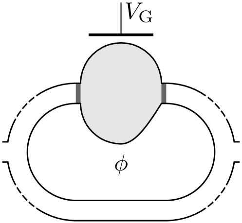
Figure 1: Aharonov-Bohm interferometer, threaded by a flux $\phi$, with a quantum dot embedded in its upper arm. The dot is capacitively coupled to a plunger gate potential $V_{\mathrm{G}}$, which tunes its electrochemical potential, and thus changes its electronic occupancy. The unsymmetrical shape of the dot reflects the presumed lack of geometric symmetry in experimental dots. The dark segments at the entrances of the dot represent tunnel barriers. The dashed lines on the arms of the interferometer stand for a number of possible additional leads.

Refs. [Yacoby95, ] and [Schuster97, ] both work with hundreds of electrons on the QD. The experiments were performed at very low temperatures ($T\approx 80$ mK) where the temperature was estimated to be the smallest energy scale in the system. In a more recent experiment at even lower temperatures ($T\approx 30$ mK), Avinum-Kalish et al. Avinum05 investigated small QD’s with zero to few tens of electrons. Their estimations of the energy scales involved in the experiments are the following: the temperature $K_{b}T\approx 0.003$ meV, the level spacing $\Delta\approx 0.5$ meV, the level width $\Gamma\approx 0.03-0.3$ meV, and the charging energy $U=1-3$ meV. Their key observation is that, as the number of electrons on the QD is reduced from 20 down to 0, $\beta_{1}$ undergoes a crossover from the universal phase behavior regime, with regularly alternating $\pi$ jumps at and in-between CB resonances, to a mesoscopic regime where phase lapses in-between CB resonances occur in a random fashion, so that the in-phase behavior of the transmission at CB resonances gets lost. These experiments provide an important hint towards the resolution of the puzzle: candidate theories applicable in the experimental regime ($T<\Gamma<\Delta<U$ ) have to be able to explain the universal to mesoscopic crossover as the QD is depopulated.

This seminal series of works motivated further experiments. The role of the magnetic field was explored by Sigrist et al. in a AB ring with one QD embedded in each of its arms. Sigrist04 The phase of a QD in the Kondo regime was measured by Ji et al. Ji00 ; Ji02 Highly controlled experiments coupled with detailed theoretical modeling for an AB device without QD also found phase lapses for some parameter values due to scattering and reflections in the arms of the ring.Kreisbeck10

The puzzles posed by the experimental data attracted a sustained theoretical interest. Refs. [Wu98, ; Kang99, ; Aharony02, ; EntinWohlman02, ] established that, under not too restrictive constraints, $\alpha$ can be extracted from $\beta_{1}$ in multi-terminal geometries. Assuming therefore that $\beta_{1}=\alpha$, Refs. [levy00, ; taniguchi99, ; Lee99, ; kim03, ] enounced the simple rules that in non- (or weakly) interacting systems, $\pi$ phase jumps occur under the two following circumstances: (i) the electrochemical potential crosses an eigenmode of the scatterer (so that one electron is added to the QD); (ii) the transmission $t$ vanishes. For non- (or weakly) interacting systems, the universal regime of transmission phase thus implies that there is one transmission zero in-between any two consecutive CB resonances. Numerical simulations on a non-interacting disordered diffusive lattice modellevy00 however showed that transmission zeros occur in-between consecutive resonances with probability close to $1/2$. From this result it is often concluded that noninteracting theories are unable to explain the experimental data.

A mechanism based on level occupation switching initially considered in Refs. [Hackenbroich97, ; Baltin99a, ] has been repeatedly used within non-interacting Oreg07 and interacting models.Silvestrov00 ; Silvestrov07 ; Goldstein09 A Fano-like scenario is assumed to stem from a given (broadened) QD level which is much more strongly coupled to the leads than all nearby (narrow) levels. Then, while the position of CB resonance peaks is determined by the energy of the narrow levels, the conductance is dominated by the transmission through the broadened level. As $V_{\mathrm{G}}$ is varied, the narrow levels are successively populated right after the CB resonance, at which point the broadened level is abruptly depopulated. It was initially argued that level occupation switching arises from specific spatial structures of the QD,Hackenbroich97 ; Baltin99a but later works went further and suggested that it generically follows from electronic correlations.Silvestrov00 ; Silvestrov07 ; Goldstein09 ; Kim06 ; Golosov06 ; bertoni07

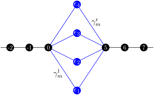
Figure 2: (Color online) Sketch of the topology of the Resonant Level Model.

More recently, lattice models for interacting fermions were numerically investigated, and an interpretation was proposed in which the electronic correlations induce the mode switching mechanism. Karrasch et al. investigated few-level, strongly interacting systems where the in-phase behavior is obtained when the single-particle level spacing on the QD becomes smaller than the level broadening due to the coupling to the leads.Karrasch07 ; Karrasch2 Varying these parameters (and the interaction strength) allowed to drive the transition between the universal and mesoscopic regime within a given dot of fixed (small) size and number of electrons, unlike the experimental case where the transition is obtained by changing the electron number and thus the filling of the dot. The mode-switching mechanism becomes relevant when the electronic population is large enough to justify a mean-field treatment of interactions. This conclusion is somehow at odds with the numerical results of Ref. [levy00, ], given that a mean-field approximation essentially delivers a single-particle theory.

Bergfield et al. considered strongly correlated models of molecules, where the universal behavior of the phase cannot be reached, unless spatial symmetries are imposed on the molecule itself and the molecule-lead couplings.Bergfield10 This latter result indicates that the universal regime requires irregular single-particle spectra, very different from regular molecular orbital spectra. Gurvitz proposed that the phase behavior in the transmission through a quantum dot results from the formation of a Wigner molecule.Gurvitz08

In another line of work, a very simple solution to the puzzle posed by Refs. [Yacoby95, ; Schuster97, ; Avinum05, ] was recently proposed.Molina12 The approach is based on the Constant Interaction Model (CIM), which treats QD in the CB regime as noninteracting, up to a constant charging energy term. The sole assumption that wave-functions have quantum chaotic spatial correlationsberry77 is able to reproduce the two main experimental observations of (i) long, universal sequences of in-phase resonances, and (ii) a crossover to a mesoscopic regime for not too large number of electrons on the QD. The probability of deviating from the universal behavior can be obtained as a function of the electron filling. Given the success of the CIM in describing different features of CB physics,Jalabert92 ; AlhassidRMP2000 it was expectable that the statistical behavior of the transmission phase were also within its reach.

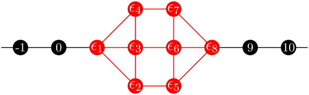
Figure 3: (Color online) Lattice model for a QD with $M=8$ sites (red) connected to two external one-dimensional leads (black).

To bring the experimental-theoretical controversy to closure, it is nevertheless important to develop and investigate more realistic models incorporating electron-electron interactions beyond the CIM (in particular including strong correlations), and check if they also can reproduce the experimental observations, for instance via the level occupation switching mechanism. This is one of the main goals of this work. In particular, we are interested in knowing if the occurrence of transmission zeros obtained with particular models of interacting electrons can account for a genuine universal regime with in-phase behavior over long sequences of resonances. For that purpose we use two different, generic models of QD: the resonant level model (RM), describing a finite number of single-particle states with repulsively interacting electrons, individually connected to external Fermi liquid leads (see Fig. 2), and lattice models (LM) with nearest-neighbor electronic repulsion, connected to two Fermi liquid leads via two sites (see Fig. 3). Our investigations are restricted to the experimentally relevant regime of zero temperature linear response and we do not address the extreme cases of models with only one or two resonant levels nor situations in which Kondo physics is relevant.Ji00 ; Ji02 ; Karrasch2

We use the DMRG-based embedding method to extract the transmission properties of the systemmolina03 ; molina04 ; MeSch03 and its recent extension to calculate the transmission phase.Molina12a We review such an approach in Appendix A and illustrate its power for a one-dimensional interacting quantum wire, including a numerical verification of the Friedel sum rule in Appendix B.

The manuscript is organized as follows. In Sec. II we introduce the one-particle version of the lattice and resonant models that we use throughout the paper. Following the standard literature, we relate the transmission zeros to a matrix resolvent and to the distribution of the coupling widths, which allows to identify the different situations in which a transmission zero can appear. Although such an analysis is not directly applicable when correlations are present, it can be extended to the many-particle case whenever an effective single-particle theory can be constructed. Furthermore, we will present numerical evidences that the behavior observed in one-particle models often also applies to strongly correlated cases. The many-particle RM is defined and studied in Sec. III. Results in the limit of large resonance widths are shown, where new zeros appear but no in-phase behavior of neighboring resonances is achieved. The next Sec. IV is devoted to many-particle lattice models, where examples are shown for different sizes and ratios between the one-particle level spacing and the level width. No significant trend towards universal behavior emerges upon inclusion of correlation effects. Finally, some conclusions and perspectives are discussed in Sec. V.

II Transmission zeros in one-particle models

Lattice models of a one-particle QD connected to one-dimensional leads were first used by Levy-Yeyati and Büttikerlevy00 for the numerical calculation of the transmission phase. The one-particle resonant level model, where the eigenstates of the QD are linked to one-dimensional leads through hopping amplitudes, was solved in Ref. [Aharony02, ] and the necessary conditions for the appearance of transmission zeros were determined. These two models have been extremely useful for discussing the behavior of the transmission phase in the non-interacting case, as well as when electron-electron interactions are treated within the CIM or at the mean-field level. In addition, both models can be further generalized to fully account for interactions by adding a Coulomb term coupling the non-interacting basis states. This is the route that we follow in Sections III and IV, and thus we start by presenting the main concepts concerning one-particle models that will be later generalized to describe the interacting case. Moreover, our discussion of one-particle models will help to systematize and classify the various approaches previously proposed to analyze the existence of transmission zeros.

An arbitrarily-shaped, non-interacting QD with $M$ sites, connected to one-dimensional leads through its 1^st and $M$^th sites, as sketched in Fig. 3, is generically described by the Hamiltonian

$$H=H_{\mathrm{D}}+H_{\mathrm{G}}+H_{\mathrm{C}}+H_{\mathrm{L}}.$$ (2)

The left and right lead Hamiltonians are given by

$$H_{\mathrm{L}}=-\sum_{i=-\infty}^{0}\left(c^{\dagger}_{i+1}c^{\phantom{\dagger}}_{i}+h.c.\right)-\sum_{i=M+1}^{\infty}\left(c^{\dagger}_{i+1}c^{\phantom{\dagger}}_{i}+h.c.\right)\,.$$ (3)

$c_{i}^{\phantom{\dagger}}$ ($c_{i}^{\dagger}$) indicate the standard operators for annihilation (creation) of a spinless fermion on site $i$ and h.c. stands for the Hermitean conjugate. We have chosen throughout this work the hopping amplitude in the leads to be the unit of energy.

Within the lattice model, the QD Hamiltonian reads

$$H_{\mathrm{D}}^{\mathrm{LM}}=-t_{\mathrm{D}}\sum_{\left<ij\right>}\left(c^{\dagger}_{j}c^{\phantom{\dagger}}_{i}+h.c.\right)+\sum_{i=1}^{M}\epsilon_{i}n_{i},$$ (4)

where $\left<ij\right>$ denotes a pair of nearest neighbor lattice sites and $n_{i}=c^{\dagger}_{i}c^{\phantom{\dagger}}_{i}$. The hopping amplitude within the dot $t_{\mathrm{D}}$ can be different from the one in the leads, and we use such a freedom in Sec. IV. In the absence of magnetic field the hopping amplitudes can be chosen to be real without loss of generality. Disorder is modeled by random on-site energies $\epsilon_{i}$, taken from a uniform distribution of width $W$.

The capacitive coupling to a nearby gate is proportional to the total number of electrons in the QD,

$$H_{\mathrm{G}}=-V_{\mathrm{G}}\sum_{i=1}^{M}n_{i}\,,$$ (5)

where capacitances are included into the definition of $V_{\mathrm{G}}$.

Since only the sites $i=1$ and $i=M$ are connected to the leads, the coupling Hamiltonian between the leads and the QD is

$$H_{\mathrm{C}}^{\mathrm{LM}}=-t_{\mathrm{C}}\left(c^{\dagger}_{0}c^{\phantom{\dagger}}_{1}+c^{\dagger}_{1}c^{\phantom{\dagger}}_{0}\right)-t_{\mathrm{C}}\left(c^{\dagger}_{M+1}c^{\phantom{\dagger}}_{M}+c^{\dagger}_{M}c^{\phantom{\dagger}}_{M+1}\right).$$ (6)

The left and right hopping amplitudes connecting the leads to the QD could in principle be different from that of the leads in order to achieve the regime of weak coupling. However, we will restrict ourselves to $t_{\mathrm{C}}=1$ throughout this work. The choice of one-dimensional leads is justified since in the tunneling regime characterizing CB physics, only a single transverse mode per lead is relevant.AlhassidRMP2000

Having defined our one-particle lattice model, we next follow Ref. [levy00, ] and discuss the conditions under which a transmission zero occurs between two resonances. Our starting point is the retarded Green’s function of the QD, which can be written as

$$G(\epsilon)=(\epsilon-H_{\mathrm{D}}-\Sigma(\epsilon))^{-1},$$ (7)

with the self-energy $\Sigma(\epsilon)$ arising from the coupling to the leads. The transmission amplitude is related to the Green’s function via the Fisher-Lee relation FisherLee

$$t(\epsilon)=i\hbar(v_{\mathrm{l}}v_{\mathrm{r}})^{1/2}G_{1M}(\epsilon),$$ (8)

where $v_{\mathrm{l(r)}}$ is the velocity in the left (right) lead for electrons with energy $\epsilon$. When leads are connected to a single QD site, the condition for having $t=0$ can be written as levy00

$${\cal C}_{1M}\left\{\epsilon-H_{D}+\Sigma(\epsilon)\right\}=0$$ (9)

where ${\cal C}_{1M}\{A\}$ stands for the cofactor of the $(1,M)$ matrix element of $A$. Since $\Sigma_{11}$ and $\Sigma_{MM}$ are the only non-zero elements of the matrix $\Sigma$, the condition expressed in Eq. (9) is entirely determined by the properties of the isolated QD and is thus independent of the coupling strength to the leads. This important observation allows us to locate the transmission zeros from those of the matrix element

$${\cal F}_{1M}(\epsilon)=\sum_{m}\frac{\psi_{m}(1)\psi_{m}(M)}{\epsilon-\epsilon_{m}},$$ (10)

of the resolvent for the isolated QD, where $\epsilon_{m}$ and $\psi_{m}(1)$($\psi_{m}(M)$) are the $m^{\rm th}$ QD’s eigenenergy and eigenfunction evaluated at site $1(M)$, respectively.

The structure of ${\cal F}_{1M}(\epsilon)$ is characteristic of physical situations where resonances are coupled to a continuum, and allows to determine the existence of zeros according to the residues of the poles. As we will see, the resonant model, that we present below, leads to equivalent conditions.

The one-particle resonant level model is obtained after a basis transformation of the QD’s degrees of freedom from the site basis to the QD’s eigenbasis. The Hamiltonian in Eq. (2) retains the same structure, with however new QD and coupling terms,

$$H_{\mathrm{D}}^{\mathrm{RM}} = \sum_{m=1}^{M}\epsilon_{m}n_{m}\,,$$ (11)

$$H_{\mathrm{C}}^{\mathrm{RM}} = \sum_{m=1}^{M}\left(\gamma_{m}^{\mathrm{l}}d^{\dagger}_{m}c^{\phantom{\dagger}}_{0}+\gamma_{m}^{\mathrm{r}}d^{\dagger}_{m}c_{M+1}+h.c.\right)\,.$$ (12)

The new fermionic operators $d_{m}=\sum_{n}\psi_{m}(n)c_{n}$ are obtained from the old ones via a unitary transformation with the eigenfunctions $\psi_{m}$ of $H_{\mathrm{D}}^{\mathrm{LM}}$, and $n_{m}=d^{\dagger}_{m}d_{m}$. In this way the levels $\epsilon_{m}$ are understood as eigenvalues of an isolated QD. Alternatively they can be interpreted as the on-site energies of a tight-binding model with the topology of Fig. 2 and hopping amplitudes given by the partial-width amplitudes $\gamma_{m}^{\mathrm{l,r}}$. The total widths are $\Gamma_{m}=|\gamma_{m}^{\mathrm{l}}|^{2}+|\gamma_{m}^{\mathrm{r}}|^{2}$.

An exact solution for the transmission amplitude in this model was presented in Ref. [Aharony02, ], which obtained

$$t(\epsilon)=\frac{2i\,f_{\mathrm{lr}}\sin{k}}{(f_{\mathrm{ll}}+e^{-ik})(f_{\mathrm{rr}}+e^{-ik})-|f_{\mathrm{lr}}|^{2}},$$ (13)

where $k$ is the wave-vector in the lead and

$$f_{\mathrm{xy}}(\epsilon)=\sum_{m}\frac{\gamma^{\mathrm{x}}_{m}\gamma^{*\mathrm{y}}_{m}}{\epsilon-\epsilon_{m}},$$ (14)

for $\mathrm{x},\mathrm{y}=\mathrm{l},\mathrm{r}$. With one-dimensional leads the partial amplitudes are proportional to the values of the resonant wave-functions at the extreme points. Therefore, $f_{\mathrm{lr}}(\epsilon)$ is simply proportional to the function $\mathcal{F}_{1M}(\epsilon)$ of Eq. (10) and to the $R$-matrix element of the corresponding scattering problem.AlhassidRMP2000 ; Jalabert92

When there are only small variations in the values of the wave-functions on the sites connecting to the leads, the behavior of ${\cal F}_{1M}(\epsilon)$ away from $\epsilon_{m}$ is dictated by the two surrounding singularities. On the other hand, large fluctuations of $\psi_{m}(1)\psi_{m}(M)$ among different $m$ might lead to values of ${\cal F}_{1M}(\epsilon)$ determined by far-away resonances. These two possible situations will be respectively referred to as Restricted Off-Resonance (ROR) behavior and Unrestricted Off-Resonance (UOR) behavior. This distinction plays a key role within the analysis of transmission phases.Hackenbroich97 ; Baltin99a ; kim03 ; Silvestrov00 ; Silvestrov07 Since large wave-function fluctuations in generic systems are rare, we will find that the ROR is the most commonly encountered scenario. Interestingly, the above classification is not only relevant for the one-particle models, but also for many-particle models (Secs. III and IV).

The existence of a transmission zero between the $m$^th and the $(m+1)$^st resonances depends on the sign of levy00 ; Silva02

$$D_{m}=\psi_{m}(1)\psi_{m}(M)\psi_{m+1}(1)\psi_{m+1}(M)\,.$$ (15)

In the ROR case, when $D_{m}>0$ (equal parity of the resonances) there is one zero between the resonances while for $D_{m}<0$ (opposite parity) there is no zero. This sign rule has been at the basis of several studies of the transmission phase. In the UOR case we have that for $D_{m}>0$ there is an odd number of transmission zeros between the $m$^th and $(m+1)$^st resonances, yielding an accumulated phase of $\pi$ between the two resonances. For $D_{m}<0$ there is no transmission zero or there is an even number of zeros, resulting in zero total phase shift between the two resonances. In the interferometric experiments on QDs operating in the CB regime it is extremely difficult to follow the transmission phase across the conductance valleys, and only the total phase between resonances is relevant. Therefore, the sign rule is also useful in the UOR case. At this point it is important to remark that the occupation switching mechanism is based on a large fluctuation of the partial width leading to the UOR behavior. As we have seen, the appearance of transmission zeros when $D_{m}<0$ is indeed possible in the UOR case, but they are bound to come in pairs, without altering the in-phase relationship of adjacent resonances.

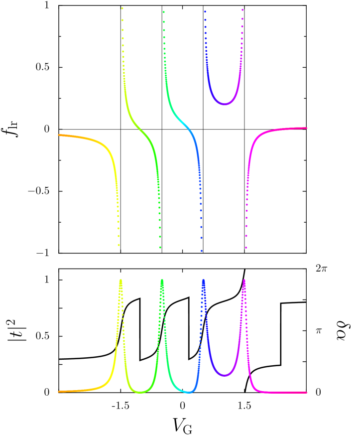
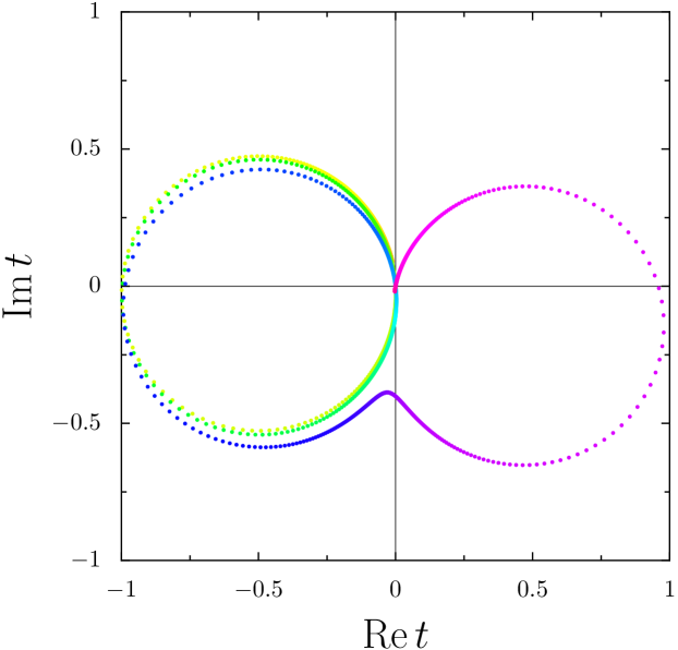
Figure 4: (Color online) Numerically obtained data for a four-resonance one-particle resonant level model with $\epsilon_{m}=m-2.5$, $\gamma^{\mathrm{l}}_{m}=\gamma^{\mathrm{r}}_{m}=0.2$ for $m=1,2,3$ and $\gamma^{\mathrm{l}}_{4}=-\gamma^{\mathrm{r}}_{4}=0.2$, exhibiting ROR behavior in all intervals. Top panel: $f_{\mathrm{lr}}$ (defined in Eq. 14). Middle panel: Transmission coefficient $|t|^{2}$ (colored data points) and phase $\alpha$ (solid black line) as a function of $V_{\mathrm{G}}$. Bottom panel: trajectories of the transmission amplitude in the complex plane when $V_{\mathrm{G}}$ is varied as on the other panels. The color rainbow scale gives the correspondence between data in different panels.

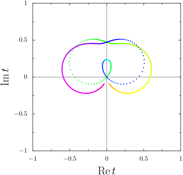
Figure 5: (Color online) Numerically obtained data for a four-resonance one-particle resonant level model with $\epsilon_{m}=m-2.5$, $\gamma_{1}^{\mathrm{l}}=\gamma_{4}^{\mathrm{l}}=-0.6$, $\gamma_{2}^{\mathrm{l}}=\gamma_{3}^{\mathrm{l}}=\gamma_{4}^{\mathrm{r}}=-0.2$, $\gamma_{2}^{\mathrm{r}}=-0.05$, $\gamma_{3}^{\mathrm{r}}=0.05$, and $\gamma_{1}^{\mathrm{r}}=0.2$, exhibiting UOR behavior between the 2^nd and 3^rd resonance. The same conventions as in Fig. 4 are adopted.

We next discuss the ROR-UOR competition and the sign rule in the one-particle RM. The experience gained in this simple one-particle situation will prove very useful for understanding the many-particle results in the next sections. Compared to the LM, the RM has the advantage that partial-width coupling amplitudes $\gamma_{m}^{\mathrm{l,r}}$ can be tuned at will. This flexibility has been a key ingredient in several theoretical works.Baltin99a ; Silvestrov00 ; Silvestrov07 ; Golosov06 ; Karrasch07 ; Karrasch2

We first show in Fig. 4 results for a system with four equidistant resonances and coupling parameters $\gamma^{\mathrm{l}}_{m}=\gamma^{\mathrm{r}}_{m}=0.2$, for all $m=1,2,3,4$, with the exception of $\gamma^{\mathrm{r}}_{4}=-0.2$. The values of the couplings all have the same magnitude, thus leading to ROR behavior. The upper panel of Fig. 4 shows the resulting function $f_{\mathrm{lr}}$ when varying the gate voltage $V_{\mathrm{G}}$ (which is equivalent to varying the energy $\varepsilon$ of the incoming particles from the lead) in arbitrary units. The middle panel of Fig. 4 shows the transmission coefficient $|t|^{2}$ and the phase $\alpha$ as a function of $V_{\mathrm{G}}$. We can see that the presence and the absence of zeros between resonances is clearly correlated with the sign of $D_{m}$. Transmission resonances and zeros correspond, respectively, to singularities and zeros of $f_{\mathrm{lr}}$. The trajectory of the transmission amplitude in the complex plane as a function of $V_{\mathrm{G}}$ is shown in the bottom panel. The trajectories crossing the origin of the complex $t$-plane occupy only one half-plane for the first three resonant peaks, and are characteristic of adjacent resonant peaks with in-phase behavior.taniguchi99 Even in this simple example there is an anomalous extra transmission zero at $V_{\mathrm{G}}\approx 2.3$ far away from the area of resonance peaks. This is a finite-size effect, arising from zeros of $f_{\mathrm{xy}}$ that lie outside the interval where the resonances are concentrated. Such a behavior is irrelevant for CB experiments with many resonances, and we only note that, according to our nomenclature, it is an UOR behavior, as the value of the transmission far from resonance is dominated by the contribution from several resonant tails. Such an effect is commonly encountered in finite size numerical simulations and it is discussed for instance in Ref.[Karrasch07, ].

Typical UOR behavior is shown in Fig. 5, where we reduced the values of the two central resonance widths to make the behavior of $f_{\textrm{lr}}$ between the second and third resonances dominated by the external resonances. A loop is formed by the trajectory in the complex plane and two new zeros appear. These zeros add phase lapses smaller than $\pi$ in the region between two resonances. The peak appearing around $V_{\mathrm{G}}=0$ is related to a small loop close to the origin of the $t$-plane and an accumulated phase smaller than $\pi$. Therefore, it does not represent a new resonance. Instead, it is the result of a broad resonance being cut by the extra Fano-like anti-resonances. We will see that similar behaviors are also found in the many-particle case where the universal behavior is not reached.

A critical UOR-ROR case arises when the two zeros of $f_{\mathrm{lr}}$ collapse in a double zero (with a horizontal tangent) yielding a kink at the origin of the complex $t$-plane with a phase shift smaller than $\pi$ (not shown). This special zero is found for specific settings of the parameters and if the couplings are perturbed infinitesimally away from that singular setting, we find either no zero or two zeros in the transmission.

The inclusion of interactions at the CIM level opens a gap of the size of the charging energy in the one-particle spectrum between the highest occupied and the lowest unoccupied dot levels without affecting the wave-functions. The UOR behavior will then be favored since many resonances contribute in the electron and hole sectors.Baltin99b However, as explained above, the sign rule dictating the phase behavior only concerns the two nearest resonances. It is therefore important to consider more refined models including arbitrary couplings and electronic correlations. We undertake this task in the forthcoming sections and discuss the results in connection with previously proposed theories and the concepts introduced in this Section.

III Many-particle resonant level model

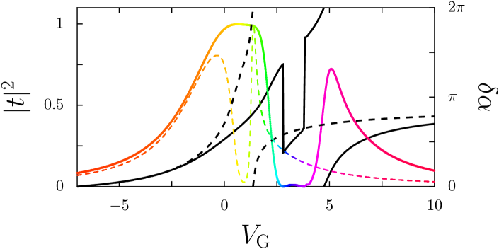
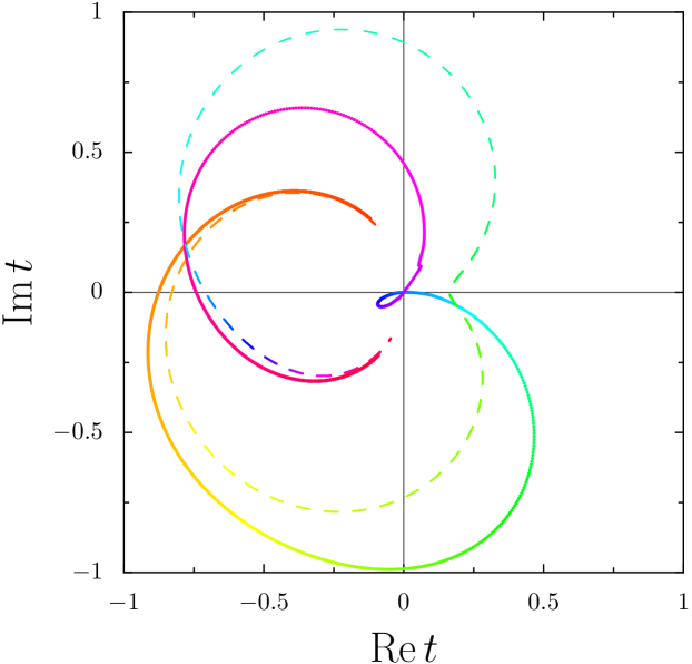
Figure 6: (Color online) Upper panel: transmission coefficient (colored) and phase (black) for non-interacting ($U=0$, dashed) and interacting ($U=2$, solid) resonance level models with three levels and parameters $\epsilon_{1}=-0.5$, $\epsilon_{2}=0.5$, $\epsilon_{3}=1.5$, $\gamma_{1}^{\mathrm{l}}=1.0$, $\gamma_{1}^{\mathrm{r}}=1.0$, $\gamma_{2}^{\mathrm{l}}=-0.5$, $\gamma_{2}^{\mathrm{r}}=0.5$, $\gamma_{3}^{\mathrm{l}}=0.4$, $\gamma_{3}^{\mathrm{r}}=0.7$ Lower panel: trajectory of the transmission in the complex plane following the convention of the last three figures.

The one-particle resonant level model is particularly useful to investigate the possibility of UOR behavior, because partial widths can be tuned at will. Since interactions at the CIM level do not favor the universal behavior of the phases, it is natural to ask whether correlation effects beyond mean field could be responsible for the experimentally observed universal behavior. This question has been analyzed by Karrasch et al., Karrasch07 via numerical investigations of many-particle resonant level models with up to $M=4$ levels and arbitrary level-lead couplings. They identified several regimes, determined by three energy scales: the mean level-width $\Gamma$, the mean one-particle level spacing $\Delta$ in the QD, and the strength of the electron-electron interactions $U$. In the case $\Gamma\lesssim\Delta$, interactions were not found to affect the behavior of transmission phases. In contrast, when $U\simeq\Gamma>\Delta$, sufficiently strong correlations appeared to favor the appearance of additional transmission zeros not predicted by the sign rule. This result was interpreted as the signature of Fano-like antiresonances between a renormalized wide resonance with several narrow single-particle levels, thus providing some justification for the level occupation switching mechanism. While the phase lapses reported in Ref. [Karrasch07, ] seem consistent with the universal regime, it is not so obvious that the zero-temperature gate-voltage dependence of the transmission reproduces the experimentally observed standard CB resonances obtained from the amplitudes of the AB oscillations in the universal regime. This is due to an incomplete filling of the resonances in the theoretical model resulting in an associated phase accumulation smaller than $\pi$, as we demonstrate below.

To better understand correlation effects on the transmission phase we reproduced and extended the results of Ref. [Karrasch07, ], working with up to $M=6$ levels in the QD. For $M=2$ and 4 our numerical calculations using the embedding technique (with Density Matrix Renormalization Group calculations) are in very good quantitative agreement with those obtained in Ref. [Karrasch07, ] with the Numerical Renormalization Group and the Functional Renormalization Group algorithms. The QD Hamiltonian of the many-particle resonant model is that of Eq. (11) plus an interaction term

$$H_{\mathrm{DU}}^{\mathrm{RM}}=\frac{U}{2}\sum_{m\neq m^{\prime}}\left(n_{m}-\frac{1}{2}\right)\left(n_{m^{\prime}}-\frac{1}{2}\right)\,.$$ (16)

In Fig. 6 we show that interactions can generate transmission zeros in dots with $\Gamma>\Delta$ already for $M=3$ states. The fluctuations of the level-widths are small enough that the non-interacting case (dashed lines) exhibits pure ROR behavior. According to the sign rule, and since there are alternating parities between consecutive resonances, there is no transmission zero. The broad peak (around $V_{\mathrm{G}}=-1$) of the non-interacting case (top panel, dashed lines) is the result of the overlap of two nearby resonances. In the interacting case with $U=2$ (top panel, solid lines), three peaks (around $V_{\mathrm{G}}=0$, 3, and 5) can be seen. Two zeros are clearly identified from the phase lapses of $\alpha$ and from the trajectories of $t$ in the complex plane (bottom panel). The small peak between the two zeros corresponds to a small loop in the complex $t$-plane, indicating the emergence of UOR behavior induced by interactions. The increase of $\alpha$ through each of the peaks is smaller than $\pi$, which would be the expected value if one electron were added to the QD.

Our example is consistent with the mechanism put forward by Karrasch et al. [Karrasch07, ], where the transmission amplitude in the vicinity of a new zero is not determined by the two nearest resonances but by an anomalously broadened level. However, the transmission phase change from one of the new zeros to the next one does not correspond to the full addition of an electron on the QD. As a direct consequence, the $V_{\mathrm{G}}$-dependence of the conductance diverges from the typical CB peak structure. We observed similar behavior in all the realizations where extra zeros appeared with interactions. The analysis of these simple cases illustrates the usefulness of the discussion presented in the previous section. Even if the function $f_{\mathrm{lr}}(\varepsilon)$ of Eq. (14) does not have meaning in a many-body situation, the concepts of ROR and UOR behavior can be addressed by varying $V_{\mathrm{G}}$ and studying the resulting trajectory in the complex $t$-plane.

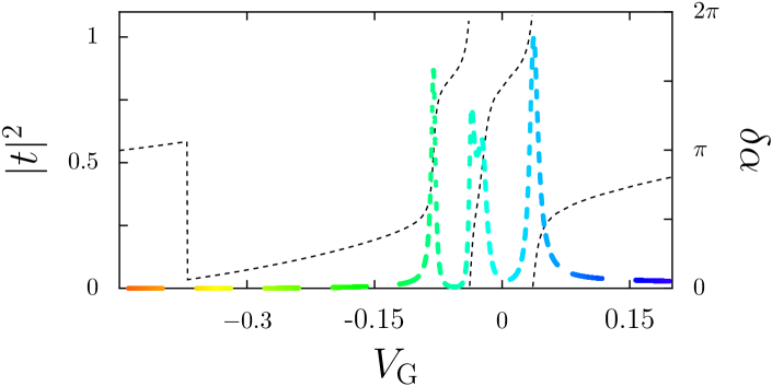
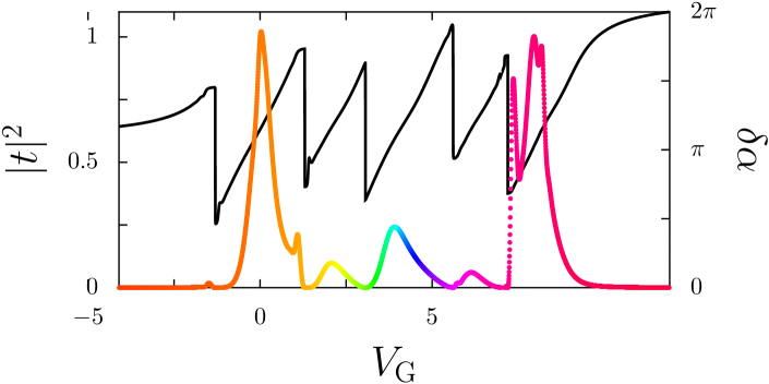
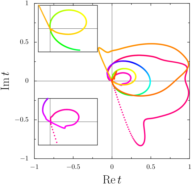
Figure 7: (Color online) Transmission coefficient (color) and transmission phase (black) of a RM with six levels for $U=0$ (upper panel, dashed) and $U=2$ (center and lower panels, solid lines and data points). The model parameters are $\epsilon_{1}=-0.113$, $\epsilon_{2}=-0.071$, $\epsilon_{3}=-0.059$, $\epsilon_{4}=0.004$, $\epsilon_{5}=0.016$, $\epsilon_{6}=0.082$, $\gamma_{1}^{\mathrm{l}}=0.3883$, $\gamma_{1}^{\mathrm{r}}=0.1775$, $\gamma_{2}^{\mathrm{l}}=-0.2106$, $\gamma_{2}^{\mathrm{r}}=0.3292$, $\gamma_{3}^{\mathrm{l}}=0.2448$, $\gamma_{3}^{\mathrm{r}}=0.1214$, $\gamma_{4}^{\mathrm{l}}=0.2581$, $\gamma_{4}^{\mathrm{r}}=-0.1936$, $\gamma_{5}^{\mathrm{l}}=0.3155$, $\gamma_{5}^{\mathrm{r}}=0.2332$, $\gamma_{6}^{\mathrm{l}}=0.4253$, $\gamma_{6}^{\mathrm{r}}=-0.1977$. The ratio between the average energy spacing and the average level width is $\Delta/\Gamma=0.26$. Bottom panel: trajectories of the transmission amplitudes in the complex plane as a function of $V_{\mathrm{G}}$. The insets show $V_{\mathrm{G}}$-intervals where transmission zeros occur together with overlapping resonances.

The advantage of our DMRG-based embedding method is that it allows to increase the QD size to larger values than previously studied, still keeping a good precision. We next extend the above analysis to larger systems, to investigate the possible crossover between the mesoscopic and the universal regime of the transmission phase. In all examples to be discussed, we randomly chose the widths $\gamma_{m}^{\mathrm{l(r)}}$, while tuning the values of the resonance energies $\epsilon_{m}$ in order to achieve different behavior in particular examples.

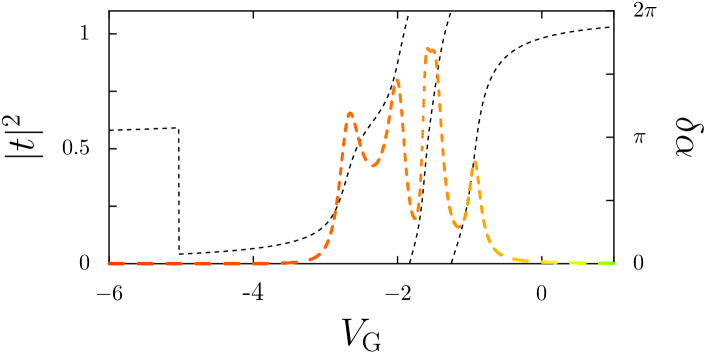
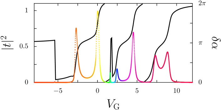
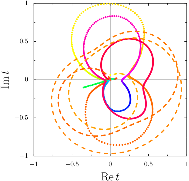
Figure 8: (Color online) Transmission coefficient (color) and transmission phase (black) of a RM with six levels for $U=0$ (upper panel, dashed) and $U=2$ (central panel, solid). The coupling amplitudes are the same as in Fig. 7, while the one-particle energies are $\epsilon_{1}=-1.7497$, $\epsilon_{2}=-1.0161$, $\epsilon_{3}=-0.6483$, $\epsilon_{4}=-0.4684$, $\epsilon_{5}=0.0428$, and $\epsilon_{6}=0.16212$, giving $\Delta/\Gamma=2.16$. Bottom panel: Trajectory of the transmission amplitude in the complex plane as a function of $V_{\mathrm{G}}$.

We show in Fig. 7 data for a QD with $M=6$ resonant levels, where the average energy spacing is much smaller than the average level width $\Delta\ll\Gamma$. The fluctuations of the coupling amplitudes are not strong enough to induce UOR behavior in the non-interacting case. The sign rule in the ROR case dictates the absence of transmission zeros between the resonances (upper panel), and there is one zero outside the region of the resonances. For $U=2$ (central panel) there is one transmission zero outside the region of the resonances and four zeros in the region of the resonances. In the same way as the previous example of a smaller QD, the phase evolution does not exhibit in-phase behavior from one resonance peak to the next, due to the non-integer filling of the dot at each resonance. The trajectory of the transmission in the complex $t$-plane shows loops typical of UOR behavior. For instance, the two resonances close to $V_{\mathrm{G}}=0$ are associated with a phase increase larger than $\pi$, and are “cut” by a zero at $V_{\mathrm{G}}\simeq 1$. The insets in the lower panel show loops between two zeros that are characteristic of conductance peaks that do not represent a resonance with the corresponding integer filling of the dot. The phase evolution in the loop is then smaller than $\pi$, and the angle of the crossing of the trajectories at the origin directly gives the missing dot filling.

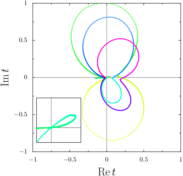
Figure 9: (Color online) Results for a resonance level model with six levels and the same parameters as in Fig. 8, at the interaction strength $U=4$. Top panel: Transmission coefficient (colored line/data points) and phase (black line). Bottom panel: Trajectory of the transmission in the complex plane as a function of $V_{\mathrm{G}}$. The inset shows the $V_{G}$ interval where the transmission zeros occur together with overlapping resonances.

We next explore the emergence of UOR behavior by taking different ratios of $\Gamma/\Delta$ within the various resonances of a given sample, considering the influence of the interaction strength $U$. We present results for a QD with $M=6$ resonant levels, where the energy spacing between the upper two levels is much smaller than all other spacings for different interaction strengths: $U=0$ and 2 (Fig. 8) and $U=4$ (Fig. 9). For $U=0$ (dashed lines) we are in the regime of overlapping resonances. This is clearly indicated by the transmission probability in the top panel of Fig. 8. There is an anomalous transmission zero outside the resonance area, arising from the same mechanism as discussed in Sec. II. The sample shows ROR behavior at $U=0$, and in agreement with the sign rule, there is no transmission zero. When the interactions are turned on, the charging energy leads to the separation of resonances, which evolve into CB peaks. Resonances no longer overlap, except the last two, whose energy separation in the non-interacting case is particularly small. The change in the behavior of the trajectory of the transmission amplitude in the complex plane induced by the effect of the interactions is remarkable. Two new zeros appear rather close to each other between the second and the third resonance thus exhibiting UOR behavior with a vanishing accumulated phase shift (see insets of the lower panels). They are located in the region where the phase evolution is driven by the beginning of the filling of the third level. No new zeros appear between the most overlapping last two resonances. As the interaction is increased further the qualitative behavior and the number of zeros is not changed. We show in Fig. 9 the results for stronger interaction strength, $U=4$, where the main difference is that CB peaks become narrower and more distant. The two zeros between the second and the third CB peak also become more separated by the effect of the increasing interaction. We checked for $U=6$ and 8 (not shown) that, except for this trivial effect, the trajectories of $t$ in the complex plane almost do not change with $U$.

In a last example of the resonant model, we kept the same couplings as in the previous examples, while significantly reducing the level spacings to enter the regime $\Delta<\Gamma$. We see in Fig. 10 that the number of zeros does not change with respect to the interacting cases of Figs. 8 and 9, but we can obtain very small loops in the $t$-plane, resulting from the extreme UOR behavior.

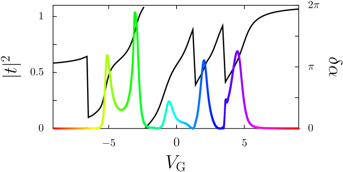
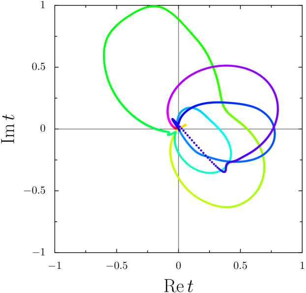
Figure 10: (Color online) Top panel: Transmission coefficient (colored line) and phase (black line) for a resonance level model with six levels and $U=2$. The coupling amplitudes are the same as in Fig. 7, while the one-particle energies are $\epsilon_{1}=-0.44976$, $\epsilon_{2}=-0.2161$, $\epsilon_{3}=-0.04683$, $\epsilon_{4}=0.0042$, $\epsilon_{5}=0.01621$, and $\epsilon_{6}=0.018$, giving $\Delta/\Gamma=0.635$. Bottom panel: Trajectory of the transmission in the complex plane as a function of $V_{\mathrm{G}}$.

The previously discussed examples show that the extrapolation towards larger systems by increasing $\Gamma/\Delta$ is delicate, and large variations of this ratio are needed in order to generate transmission zeros between each pair of consecutive resonances.

From our numerical results in the many-particle RM we conclude that (i) level occupation switching induced by interactions appears only in the extreme $\Delta\ll\Gamma$ case where the zeros can cut through resonances, and (ii) it is directly related to UOR behavior where the transmission between resonances is not simply given by the independent contributions from the nearest two resonances. There is a wide intermediate regime $\Delta\approx\Gamma$ where UOR behavior appears only for part of the resonances. The interaction must satisfy $U\gg\Delta$ and $U\gtrsim\Gamma$ for the effect to appear,Karrasch07 but once this is the case, increasing $U$ further does not induce any qualitative changes in the number of transmission zeros and the associated phase lapses. Finally, the occurrence of this mechanism should translate into a partial occupation of the dot when the special zeros induced by correlations appear. In this case, the form of the conductance peaks seems to depart significantly depart from the well resolved CB peaks observed in the universal regime.

IV Many-particle lattice models

While the RM is very useful to discuss the various possible scenarios that may lead to the appearance of transmission zeros and the associated phase lapses, the single-level energies and half-width amplitudes are independent parameters of the model. We therefore return to lattice models in this section, where the single-level parameters are determined by the geometry of the lattice system.

The dot Hamiltonian for a lattice model of spinless fermions with nearest-neighbor interaction is given by that of Eq. (4) plus the interaction term

$$H_{\mathrm{DU}}^{\mathrm{LM}}=U\sum_{\left<ij\right>}\left(n_{i}-\frac{1}{2}\right)\left(n_{j}-\frac{1}{2}\right).$$ (17)

Such a nearest-neighbor repulsion can lead to strong correlations depending on the value of the interaction strength $U$. Writing the interaction term in the basis of the one-particle dot eigenstates, it would take the form of (16), but with level-dependent interaction strengths and widths calculated from the dot eigenfunctions. The limitation to nearest-neighbor interaction considerably simplifies the numerical work, but it is not of fundamental nature.

When $U\neq 0$, it is not possible to make a priori general statements about the behavior of the zeros. We therefore performed numerical calculations using the embedding method presented in detail in the App. A. We considered systems ranging from the simplest topology of a diamond with $M=4$ sites (Fig. 1 of Ref. [Molina12a, ]) to dot sizes up to $M=8$ sites (see Fig. 3).

When the single-particle level-spacing is of the order of the level-width ($\Delta\gtrsim\Gamma$), the transmission zeros with $U\neq 0$ typically exhibit the same qualitative behavior as in the non-interacting case $U=0$ [Karrasch07, ; Molina12a, ]. This situation typically happens in small systems when $t_{\mathrm{D}}=1$. For instance, in the case with $M=4$ and on-site energies chosen such that one has a transmission zero at $U=0$, the effect of the interactions is to separate the peaks, reducing their widths without changing the qualitative behavior of the scattering phase Molina12a .

Figure 11: Transmission coefficient vs. gate voltage of a lattice model for a quantum dot with four sites and $t_{\mathrm{D}}=0.25$ for $U=0$ ($4$) in top (bottom) panel. The chosen disorder has led to on-site energies $\epsilon_{1}=0.220$, $\epsilon_{2}=0.360$, $\epsilon_{3}=0.219$, $\epsilon_{4}=-0.037$. The logarithmic scale used in the insets allows to locate the transmission zeros.

In simple models of small dots without disorder, interactions do not modify the number of transmission zeros from the non-interacting case and they do not induce a change from ROR to UOR behavior. By varying the on-site energies and taking $t_{\mathrm{D}}<1$, we occasionally obtain the displacement of a transmission zero from the region between the resonances to the zone outside the resonances. Such a behavior is shown in Fig. 11, for the case $M=4$, $t_{\mathrm{D}}=0.25$, $U=4$ and a realization of the on-site energies $\epsilon_{i}$ randomly chosen in the interval $[-W/2,W/2]$ with $W=1$. In this realization, there is a transmission zero between two groups of resonances in the case $U=4$; $t_{\mathrm{D}}=1$ and also in the non-interacting case $U=0$ when $t_{\mathrm{D}}=0.25$. However, this zero disappears in the shown case of $t_{\mathrm{D}}=0.25$ and $U=4$, while another zero appears outside the resonance area. The disappearance can be related to a change in the wave function of the dot that evolves into a charge density wave in the interacting case.

According to Ref. [Karrasch07, ], the evolution from the mesoscopic to the universal regime can be achieved if $\Delta\lesssim\Gamma\lesssim U$. To check this idea, we reached the previous condition within the many-particle LM by going to relatively large systems ($M=8$) and taking the hopping within the dot smaller than in the leads.

Systems of different sizes ($M=4$ to $8$) level spacings ($t_{\mathrm{D}}=1$ and $t_{\mathrm{D}}<1$) and interaction strengths ($U=0$ to $8$), with and without disorder, have been explored. The numerical investigations are extremely time consuming, which is why we base our analysis on $|t|$ instead of calculating the complex $t$.numericaldifficulty Below we present some illustrative examples supporting our general conclusion: interactions do not typically induce the transition from the mesoscopic to the universal regime.

Figure 12: $|t|^{2}$ vs. $V_{\mathrm{G}}$ of a lattice model for a quantum dot with $M=8$ sites and $U=0$ (4) in the top (bottom) panel. $t_{\mathrm{D}}=0.5$ and $W=1$. The inset shows the same data on a logarithmic scale.

In general, the main effect of the interaction is to separate the resonance peaks and to make them narrower. In the more common scenario the number of transmission zeros is unchanged from the non-interacting to the interacting case. In some cases, the structure of the resonances may substantially change when interactions are switched on and the position of the zeros can change accordingly. Resonances that are very close and then indistinguishable in the non-interacting case, can often be resolved in the interacting case. A scenario we have observed in several examples is the disappearance of transmission zeros beyond a given interaction strength. This situation arises because the original UOR zeros occurring in the regime $\Gamma\gg\Delta$ disappear as interactions change the ratio between $\Gamma$ and $\Delta$. Pushing a transmission zero outside the interval where the resonances are (like the example shown in Fig. 11) is another common outcome of including interactions. All cases analyzed resulted in the mesoscopic regime with a random alternation between resonances and transmission zeros and significantly less transmission zeros than resonances. In no instance did we find that interactions can induce a transition from ROR to UOR behavior as it was the case in the RM. Scaling up the system size or varying $t_{\mathrm{D}}$ and $U$ did not change these conclusions.

Figure 13: $|t|^{2}$ vs. $V_{G}$ for $U=0$ ($2$) in top (bottom) panel, of a lattice model for a quantum dot with eight sites, $t_{\mathrm{D}}=1$, and $W=1$. The inset shows the same data on a logarithmic scale.

In Fig. 12 we show an example with $M=8$, $U=2$, and $t_{\mathrm{D}}=0.5$ exhibiting the most commonly encountered behavior where the number of zeros does not change from the non-interacting to the interacting case. Even if the structure of the resonances and the position of the zeros change dramatically from one case to the other, the total number of zeros remains constant.

We finally illustrate in Fig. 13 a scenario we often observed, with less zeros in the interacting case than in the non-interacting one in a quantum dot with $M=8$, $U=2$, $W=1$, and $t_{\mathrm{D}}=1$. The double zero in the middle of the curve (around $V_{\mathrm{G}}=1$) of the $U=0$ case corresponds to an UOR case that is transformed to a normal ROR zero for $U=2$. As resonant peaks become narrower and more separated in the presence of interactions UOR behavior is not favored. This is very different from the situation in the RM, and we do not observe here the population switching mechanism.

V Conclusions

In this work, we have presented numerical investigations of the transmission phase through confined, strongly correlated electron systems. Our goal was to determine how correlation effects influence the transmission phase, and whether they are able to explain the existing experimental observations of Ref.[4,6,9,10]. In order to compute the complex transmission amplitude of the scattering matrix corresponding to strongly correlated systems we have extended the embedding method previously used for conductance computations. For the simplicity of the numerical calculations we have used a model of spinless electrons. This is appropriate since spin effects are only expected to be important for extremely small dots, while our interest is to achieve the conditions of dots large enough to reach the transition from the mesoscopic to the universal regime.

We have analyzed two different models including electron-electron interactions: the resonant level model and lattice models with nearest-neighbor interactions. The non-interacting limits of these models were also discussed in order to define different scenarios for the occurrence of transmission zeros and phase lapses. When the width of the resonances is smaller than the level spacing, the peaks are well resolved in energy. Two cases should then be considered: restricted off-resonance (ROR) behavior, in which the two nearest resonances determine the character of the transmission amplitude in-between; and unrestricted off-resonance (UOR) behavior, where the transmission amplitude between two adjacent resonances is significantly affected by other far-away resonances. In the ROR case we have one transmission zero or none, depending on the sign of $D_{m}$ [see Eq. (15)] being positive or negative, respectively. In the UOR case, and when the resonances are well separated, the number of zeros might be increased with respect to the ROR case by a multiple of two, which would not change the total phase shift accumulated in the interval between the resonances. Therefore, we have a phase shift of $\pi$ or $0$ between the resonances depending on $D_{m}$ being positive or negative, respectively.

The situation changes when the resonances are strongly overlapping and it has no meaning to treat peaks and valleys separately in the energy dependence of the transmission amplitude. In these cases the transmission is typically given by the contributions from many resonances resulting in an UOR behavior with the possible appearance of zeros. However, the phase accumulated in the region of overlapping peaks is not an integer multiple of $\pi$. The transmission zeros cut the phase evolution leading to the incomplete filling of the dot and phase shifts smaller than $\pi$. This case is clearly not representative of the experimental situation, where well-resolved peaks alternate with conductance valleys.

In the case of the resonant model we confirm previous results Karrasch07 about the possible increase in the number of zeros due to the presence of interactions in the regime of very wide resonances, depending on the choice of the coupling parameters. We relate this phenomenon to the UOR behavior studied in the non-interacting case. However, results for the RM do not fully reproduce key features of the experiment like the in-phase behavior of consecutive resonances.

We treated lattice models of dots with up to $M=8$ sites. In most of the cases the number of transmission zeros was independent of the interaction strength, while in a minority of cases we have observed that interactions can induce ROR behavior from UOR behavior as resonances become more narrow and isolated, thus reducing the number of transmission zeros. Consistently with the experimental findings, we observe the mesoscopic behavior for the small size QD that we treat numerically. In addition, when decreasing the internal hopping amplitude to achieve smaller energy level separation with respect to the level couplings, no tendency towards universality was obtained, independently of the value of the interaction strength. The exploration of a large parameter space of level separations, coupling widths, and level spacings allowed to approach the conditions of not so small QD, where the universality was claimed to arise by the effect of electronic correlations. This is not the case. Only at large enough QD ($kL_{\mathrm{S}}\gg 1$), the one-particle wave-function correlations provoke the emergence of universality, but for those relatively large sizes the electronic correlations are no longer important.AlhassidRMP2000

In the non-interacting case with chaotic underlying dynamics, the generic distribution of eigenstates and partial widths AlhassidRMP2000 favor the ROR behavior. Taking interactions at the CIM level may lead to the UOR behavior, but with well separated resonances. Therefore, in these cases the sign rule based on the one-particle wave-functions determines the phase behavior. The case of UOR with overlapping resonances is achieved by some tuning of the system parameters in the non-interacting and CIM cases.

Our main conclusion is that strong correlations cannot generically explain the experimentally observed universal behavior of transmission phases in large dots, nor the crossover from mesoscopic behavior in few-electron dots to universal behavior in many-electron dots. This result is consistent with the observationMolina12 that the emergence of the universal behavior can be obtained taking into account one-particle wave-function correlations.

Appendix A Embedding method for the transmission phase

In this appendix we reformulate the embedding approach for the transmission phase put forward in Ref. Molina12a , settling the notation and the basis of the numerical method used in Secs. III and IV. We also address the connection between scattering phase and induced charge, which are shown in App. B to provide a useful numerical test of the method beyond those used in Ref. Molina12a .

The embedding method is a powerful technique to calculate the conductance through a strongly correlated nanosystem with or without disorder.molina03 ; molina04 ; MeSch03 ; vasseur06 ; vasseurthesis ; molina05 The system of interest is connected to a one-dimensional lead that closes into itself resulting in a ring which is pierced by a magnetic field. The response of ground state properties to such a perturbation, like the persistent current or the phase sensitivity, allows to infer the conductance of the original system. While the one-dimensional setups with spinless electrons have been the most commonly used models, quasi-one dimensional leads and Hubbard chains have been recently considered,Freyn10 and nanosystems with non-trivial structure have also been studied.Moliner11 The generalization of the embedding approach to the transmission phase lies on the same basis as the original method and provides a very useful tool.

The setup of the embedding method is given by a Hamiltonian as the one of Eq. (2), where $H_{\mathrm{D}}$ stands for the Hamiltonian of the quantum dot depending on the model considered. $H_{\mathrm{G}}$ (5) allows for the application of a gate voltage, while the coupling term is given by (6) or (12). The lead Hamiltonian needs to be modified with respect to (3) in order to represent a ring pierced by a flux $\phi_{\mathrm{e}}$. It reads

$$H_{\mathrm{L}}=-\sum_{i=M+1}^{L}\left(c^{\dagger}_{i+1}c^{\phantom{\dagger}}_{i}+h.c.\right)$$ (18)

with the boundary condition $c_{0}=\exp(2\pi i\phi_{\mathrm{e}}/\phi_{0})c_{L}$. In the inset of Fig. 14 we show the embedding setup for a linear QD (a chain) as used in App. B (notwithstanding a QD of arbitrary shape like those of Figs. 3 and 2 can be treated). Despite the similarity between the embedding setup and that of the AB interferometer, they are very different since the first is a closed system with fixed number of particles and the flux $\phi_{\mathrm{e}}$ is an auxiliary one, without physical reality.

Staying at first within a one-particle model (that is, without the interaction terms (16) or (17)) and with one-dimensional leads, the transport through the nanosystem is characterized by the scattering matrix

$$S=\left(\begin{array}[]{cc}r&t^{\prime}\\ t&r^{\prime}\end{array}\right)=e^{i\zeta}\left(\begin{array}[]{cc}ie^{i\xi}\cos{\theta}&e^{i\eta}\sin{\theta}\\ e^{-i\eta}\sin{\theta}&ie^{-i\xi}\cos{\theta}\end{array}\right)\,.$$ (19)

We have chosen a generic parametrization of a $2\times 2$ unitary matrix. The transmission amplitude for particles coming from the left of the QD and as defined in the introduction is given by

$$t=|t|e^{i\alpha}=e^{i(\zeta-\eta)}\sin{\theta}\,.$$ (20)

It is related with the Green function by Eq. 8. $t^{\prime}$ is the transmission amplitude for particles impinging from the right and $r(r^{\prime})$ is the reflection amplitude for particles coming from the left (right) of the QD. The angle $\theta$ and the scattering phase $\zeta$ are restricted to the interval $[0,\pi)$, while the phases $\eta$ and $\xi$ are defined on $[0,2\pi)$.

When the Hamiltonian of the dot exhibits time-reversal symmetry, one has $\eta=0$ or $\eta=\pi$. This will be our case, since the artificial flux $\phi_{\mathrm{e}}$ used to drive the persistent current is seen by the ring, but not by the dot. When a control parameter is varied (like $V_{\mathrm{G}}$ or $\epsilon$), a jump of $\eta$ between its two possible values can only occur when the transmission amplitude vanishes ($\sin\theta=0$), in order to preserve the continuity of the scattering matrix. This observation is equivalent to that of Sec. I about the crossing of the origin of the complex plane by the transmission amplitude being typically associated with a jump of $\pi$ of its phase $\alpha$.

Right-left symmetry would restrict $\xi$ to $0$ or $\pi$. Similarly as in the case of time-reversal symmetry, jumps of $\pi$ in $\xi$ are only allowed when $\cos\theta=0$, that is, when the reflection amplitude vanishes. However, throughout this work, we consider generic QDs with arbitrary $\xi$.

When considering the phase evolution as a function of an external parameter, it is often convenient to work with the accumulated phase $\alpha_{\mathrm{c}}$, whose range of definition is not restricted to the interval $[0,2\pi)$.

Embedding the scatterer in a ring of length $L_{\mathrm{L}}$ pierced by a dimensionless flux $\Phi_{\mathrm{e}}=2\pi\phi_{\mathrm{e}}/\phi_{0}$ leads to the following quantization condition for the one-particle states of the composed systemmolina04

$$\cos(\Phi_{\mathrm{e}}-\eta)=\frac{1}{\sin{\theta}}\cos\big{(}kL_{\mathrm{L}}+\zeta\big{)}\ .$$ (21)

Since the scattering phase $\zeta$ belongs to the interval $[0,\pi)$, there are two branches for the solutions (in $k$) of (21) corresponding to the two possible values of $\eta$ (0 and $\pi$). On the other hand, the transmission phase $\alpha$ is defined in $[0,2\pi)$, which allows to write (21) in the more compact way

$$\cos(\Phi_{\mathrm{e}})=\frac{1}{\sin{\theta}}\cos\big{(}kL_{\mathrm{L}}+\delta\alpha\big{)}\ .$$ (22)

We note $L_{\mathrm{S}}$ the length of the scatterer between the leads, $L=L_{\mathrm{S}}+L_{\mathrm{L}}$ the total length of the ring, and the phase shift $\delta\alpha=\alpha-kL_{\mathrm{S}}$. We express $L$ and $k$ in Anderson units (that is, in terms of the lattice spacing). Knowing the dispersion relation in the leads $\epsilon(k)$, the sum over the energetically lowest one-body energies $\epsilon(k_{n})$ allows to obtain the ground-state energy $E(N)$ of the whole system containing $N$ particles. For an odd number of particles $N=2n_{\mathrm{F}}+1$, the lowest order terms in a $1/L$ expansion read molina04

$$E(N)=E^{(0)}(N)-\frac{2}{L}\sum_{n=1}^{n_{\mathrm{F}}}\left.\frac{\mathrm{d}\epsilon}{\mathrm{d}k}\right|_{k=k_{n}^{(0)}}\delta\alpha(k_{n}^{(0)})+O[1/L]$$ (23)

with the $k$-values in a clean ring $k_{n}^{(0)}=2\pi n/L$. The ground state energy of a clean ring (with a scatterer having perfect transmission $|t|=1$ and $\delta\alpha=0$) is given by

$$E^{(0)}(N)=\epsilon(0)+2\sum_{n=1}^{n_{\mathrm{F}}}\epsilon(k_{n}^{(0)})\,.$$ (24)

The embedding method allows to obtain the conductance of the scatterer from the flux dependence of $E(N)$, which only appears in second order in $1/L$. By changing the total number of particles, we have access, with the help of (23) and (24), to the scattering phase shift at the Fermi level ($k_{\mathrm{F}}=\lim_{L\to\infty}k_{n_{\mathrm{F}}}^{(0)}$) of the lead

$$\delta\alpha(k_{\mathrm{F}})=-\lim_{L\to\infty}\frac{L}{2}\left(\frac{E(N)-E(N-2)-2\epsilon(k_{n_{\mathrm{F}}}^{(0)})}{\left.\mathrm{d}\epsilon/\mathrm{d}k\right|_{k=k_{n_{\mathrm{F}}}^{(0)}}}\right)\,.$$ (25)

In a chain with $N=L/2+1$ (and $L$ multiple of 4) we are effectively at half filling, $k_{n_{\mathrm{F}}}^{(0)}=\pi/2$ such that Eq. 25 reduces to

$$\delta\alpha(k_{\mathrm{F}})=-\lim_{L\to\infty}\frac{L}{4}\left[E(L/2+1)-E(L/2-1)\right]\,.$$ (26)

The previous derivation is based on a single-particle approach. As in the case of the embedding method for the conductance, the passage to the many-body system is justified by the fact that the scattering properties of a many-particle scatterer can be represented by an effective one-particle scattering matrix. For instance, it has been verified molina04 ; Freyn10 that the flux-dependence of the many-particle ground state is, in the large $L_{\mathrm{L}}$ limit, reproduced by the total energy obtained from effective single-particle states (as done in the previous derivation).

In the many-body case, the scattering matrix (19) is therefore understood as an effective one, where each of its entities depends on the interaction strength $U$. This identification is made in the embedding method for the transmission phase as well as for the conductance. As a logical consequence, the results for the two quantities have to be consistent. Indeed, we obtain jumps in the transmission phase as a function of the parameters precisely at the positions where transmission zeros occur. When using Eqs. 25 or 26 in order to obtain the transmission phase, the limiting procedure is implemented by extrapolating towards large values of $L_{\mathrm{L}}$. This procedure is numerically demanding, and constitutes the bottleneck of the embedding method.molina03 ; molina04 ; Molina12a ; molina05 ; vasseur06 ; vasseurthesis ; Freyn10

The eigenphases of the scattering matrix are, for $\cos\theta\cos\xi>0$, $\varphi_{1}=\zeta+\mathrm{Arcsin}(\cos\theta\cos\xi)$ and $\varphi_{2}=\zeta+\pi-\mathrm{Arcsin}(\cos\theta\cos\xi)$, and the corresponding Wigner time is

$$\tau(\epsilon)=\frac{\hbar}{2}\sum_{q=1}^{2}\frac{\mathrm{d}\varphi_{q}}{\mathrm{d}\epsilon}=\hbar\ \frac{\mathrm{d}\zeta}{\mathrm{d}\epsilon}\ .$$ (27)

The one-particle density of states in the scattering region is related to the Wigner time as DoSm ; JP

$$d(\epsilon)=\frac{1}{\pi\hbar}\langle\tau(\epsilon)\rangle\,,$$ (28)

where the brackets stand for a spectral average over many eigenstates.

Integrating over an energy interval we recover the Friedel sum rule friedel52 ; langer61

$$\Delta\zeta=\pi\Delta N_{\mathrm{S}}$$ (29)

as a relationship between the number of particles $N_{\mathrm{S}}$ added to the scattering region and the corresponding change in the scattering phase.

The fact that the Friedel sum rule in its form (29) applies to the scattering phase $\zeta$ has been emphasized in the literature Lee99 ; levy00 ; taniguchi99 . The lapses of $\pi$ in the transmission phase $\alpha$ at the zeros of $t$ are not related with a special behavior of the density of states. However, the integration leading to (29) involves a large energy interval (on the scale of the level spacing) where many lapses appear. Since the origin of the complex plane is crossed in many different directions, the effect of the lapses tends to average out, and we can write the accumulated phase in the interval as also given by the Friedel sum rule

$$\Delta\alpha_{\mathrm{c}}=\pi\Delta N_{\mathrm{S}}\,.$$ (30)

Such an average behavior has been discussed in Ref. [Molina12, ] where the ambiguity between the lapses of $\pi$ and $-\pi$ was proposed to be lifted by applying a small magnetic field. Then, the origin in the complex $t$-plane can be avoided and well defined phase lapses with a phase change close to $\pi$ or $-\pi$ obtained. The scattering phase can then be obtained from the accumulated phase by taking $[\alpha_{\mathrm{c}}(B=0^{+})+\alpha_{\mathrm{c}}(B=0^{-})]/2$.

The existence of phase jumps in the $V_{\mathrm{G}}$-dependence of $\alpha$ can also be obtained from the standard embedding method applied to the conductance by locating the zeros of the transmission, as we do in Sec. IV. The quantization condition (21) leads to a phase sensitivitymolina04

$$\Delta E =E(N,\Phi_{\mathrm{e}}=\pi)-E(N,\Phi_{\mathrm{e}}=0)$$ (31)

$$=\frac{\hbar v_{\mathrm{F}}}{L}\left[\frac{\pi}{2}-\mathrm{Arccos}(\sin{\theta}\cos{\eta})\right]\,,$$

and therefore

$$|t|=\sin{\left(\Delta E\frac{L}{\hbar v_{\mathrm{F}}}\right)}\cos{\eta}=\sin{\left(\frac{\pi}{2}\left|\frac{\Delta E}{\Delta E^{(0)}}\right|\right)}\,,$$ (32)

where $\Delta E^{(0)}$ is the phase sensitivity of a perfectly transmitting scatterer. Since we are working with time-symmetric dots, $\eta$ can only take the values $0$ or $\pi$. The switches between these two branches may only occur when $t=0$. Therefore, the sign changes of $\Delta E$ are associated with the $\pi$ lapses in $\eta$ and $\alpha$. One should also notice that there can also be transmission zeros without phase lapses in cases when there is a zero of $\Delta E$ without a sign change. Indeed this possibility can occur for particular values of the parameters, as discussed in Sec. II.

For a strictly one-dimensional system, the sign of $\Delta E$ is fixed by Leggett’s theorem leggett ; waintal08 . For an odd number of particles we are in the branch of $\eta=0$, the transmission amplitude $t$ never vanishes, and there cannot be branch-switches or phase lapses. For a quasi-one dimensional scatterer this is no longer true, and we expect to have parameter values where $t$ vanishes and branch-switches appear.

Appendix B Transmission phase of a one-dimensional many-body scatterer

The applicability of the embedding method to obtain the transmission phase of a many-body scatterer can be conveniently tested in the one-dimensional case. As discussed at the end of A, one-dimensional systems are constrained to the branch $\eta=0$, thus $\alpha=\zeta$, and there are no transmission zeros. On the other hand, comparing the numerical results to the prediction from the Friedel sum rule constitutes a valuable test of the method.

An interacting one-dimensional chain is a particularly simple example of a many-particle lattice model where the dot Hamiltonian (Eq. 4) only has $M=L_{\mathrm{S}}$ ordered sites. For simplicity, we work in this section in the non-disordered case $\epsilon_{i}=0$ and we take $t_{\mathrm{D}}=1$. In the absence of a gate voltage $(V_{\mathrm{G}}=0)$, we work at half filling, $E(L/2+1)=E(L/2-1)$, for periodic boundary conditions in the ring and thus $\delta\alpha=0$, independent of the interaction strength. The number of electrons in the scattering region

$$N_{\mathrm{S}}=\sum_{i=1}^{L_{\mathrm{S}}}\langle n_{i}\rangle$$ (33)

is equal to $L_{\mathrm{S}}/2$. This is consistent with the findings of Ref. [molina05, ], where Fabry-Perot like oscillations of the transmission through two interacting regions in series were studied.

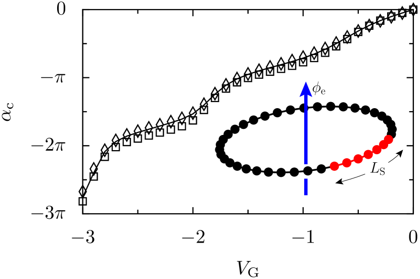
Figure 14: (Color online) Accumulated transmission phase shift for a many-body scatterer of length $L_{\mathrm{S}}=10$ with interaction strength $U=2$ (solid line), as a function of the gate voltage $V_{\mathrm{G}}$. The squares are the prediction of the Friedel sum rule based on the numerically obtained charge densities on the $L_{\mathrm{S}}$ interacting sides. The diamonds result when the densities on the $L_{\mathrm{S}}$ sites of the scatterer plus that of 10 additional sites surrounding the interacting region. The inset shows a sketch of the embedding setup for a simple one-dimensional interacting scatterer (in red).

In contrast, once an additional gate voltage is applied (Eq. 5), particle-hole symmetry is broken and $N_{\mathrm{S}}$ will differ from $L_{\mathrm{S}}/2$. The phase shift is thus expected to be nonzero. For such a setup, the embedding method has been used to show that Coulomb-blockade like oscillations of the conductance as a function of $V_{\mathrm{G}}$ appear in the presence of interactions vasseur06 even in the well coupled case. The charge in the dot region decreases in steps once $V_{\mathrm{G}}$ is increased and depletes the interacting region. We extend now these DMRG DMRG_book ; schmitteckert_thesis based calculations to compute the ground state density of rings embedding such a many-body scatterer, as well as the transmission phase resulting from (26). We choose a chain with $L_{\mathrm{S}}=10$ sites and an interaction strength $U=2$.

Data for ring sizes up to $L=120$ were used in the extrapolation towards infinite size. The results for the transmission phase are presented in Fig. 14 (solid line) together with $\pi N_{\mathrm{S}}-\pi L_{\mathrm{S}}/2$ (squares).

Both quantities should be equal according to the Friedel sum rule since $\delta\alpha=\alpha-\pi L_{\mathrm{S}}/2$ for half filling. The results have very similar behavior but small quantitative differences appear.

The difference disappears when the density modifications outside the $L_{\mathrm{S}}$ sites of the scattering region are included in the calculation of $N_{\mathrm{S}}$. Taking into account the density changes in the interacting region plus that on 5 additional sites on either side of the scatterer (diamonds), the values of $\pi N_{\mathrm{S}}-\pi L_{\mathrm{S}}/2$ are in quantitative agreement with those of $\delta\alpha$.

From this numerical example we have learned how precise the embedding method for scattering phases is, and we have checked that in order to comply with the Friedel sum rule, all the charge displacement in the neighborhood of the scatterer has to be accounted for. The effect of the charge build-up in the leads of the AB interferometer was invoked in Ref. [levy95, ] as an important ingredient in order to address the physics of the experimentally observed in-phase behavior of consecutive resonances. This kind of charge displacement and screening effects might be responsible for the phase increase smaller than $\pi$ at certain resonances which is observed in the experimental data.Schuster97

The embedding method is particularly efficient when dealing with one-dimensional leads molina04 ; Freyn10 , but the scatterer might have any topology or dimensionality. Upon this fact is based our numerical work of Secs. III and IV where the quasi-one dimensional systems that allow transmission zeros are thoroughly studied.

References

- (1) Y. Imry, Introduction to Mesoscopic Systems (Oxford University Press, Oxford, 2002), 2nd ed.
- (2) R. Landauer, Philos. Mag. 21, 863 (1970).
- (3) M. Büttiker, Phys. Rev. Lett. 57, 1761 (1986).
- (4) A. Yacoby, M. Heiblum, D. Mahalu, and H. Shtrikman, Phys. Rev. Lett. 74, 4047 (1995).
- (5) A. Levy Yeyati and M. Büttiker, Phys. Rev. B 52, R14360 (1995).
- (6) R. Schuster, E. Buks, M. Heiblum, D. Mahalu, V. Umansky, and H. Shtrikman, Nature 385, 417 (1997).
- (7) A. Aharony, O. Entin-Wohlman, B.I. Halperin, and Y. Imry, Phys. Rev. B 66, 115311 (2002).
- (8) O. Entin-Wohlman, A. Aharony, Y. Imry, Y. Levinson, and A. Schiller, Phys. Rev. Lett. 88, 166801 (2002).
- (9) M. Avinum-Kalish, M. Heiblum, O. Zarchin, D. Mahalu, and V. Umansky, Nature 436, 529 (2005).
- (10) M. Sigrist, A. Fuhrer, T. Ihn, K. Ensslin, S.E. Ulloa, W. Wegscheider, and M. Bichler, Phys. Rev. Lett. 93, 066802 (2004).
- (11) Yang Ji, M. Heiblum, D. Sprinzak, D. Mahalu, and Hadas Shtrikman, Science 290, 779 (2000).
- (12) Yang Ji, M. Heiblum, and Hadas Shtrikman, Phys. Rev. Lett. 88, 076601 (2002).
- (13) C. Kresisbeck, T. Kramer, S.S. Buchholz, S.F. Fischer, U. Kunze, D. Reuter, and A.D. Wieck, Phys. Rev. B 82, 165329 (2010).
- (14) J. Wu, B.-L. Gu, H. Chen, W. Duan, and Y. Kawazoe, Phys. Rev. Lett. 80, 1952 (1998).
- (15) K. Kang, Phys. Rev. B 59, 4608 (1999).
- (16) A. Levy Yeyati and M. Büttiker, Phys. Rev. B 62, 7307 (2000).
- (17) T. Taniguchi and M. Büttiker, Phys. Rev. B 60, 13814 (1999).
- (18) H.-W. Lee, Phys. Rev. Lett. 82, 2358 (1999).
- (19) T.-S. Kim and S. Hershfield, Phys. Rev. B 67, 235330 (2003).
- (20) G. Hackenbroich, W.D. Hwiss, and H.A. Weidenmüller, Phys. Rev. Lett. 79, 127 (1997).
- (21) R. Baltin, Y. Gefen, G. Hackenbroich, and H.A. Weidenmüller, Eur. Phys. J. B 10, 119 (1999).
- (22) Y. Oreg, New J. Phys. 9, 122 (2007).
- (23) P.G. Silvestrov and Y. Imry, Phys. Rev. Lett. 85, 2565 (2000).
- (24) P.G. Silvestrov and Y. Imry, New J. Phys. 9, 125 (2007).
- (25) M. Goldstein, R. Berkovits, Y. Gefen, and H.A. Weidenmüller, Phys. Rev. B 79, 125307 (2009).
- (26) S. Kim and H. W. Lee, Phys. Rev. B 73, 205319 (2006).
- (27) D.I. Golosov and Y. Gefen, Phys. Rev. B 74, 205316 (2006).
- (28) A. Bertoni and G. Goldoni, Phys. Rev. B 75, 235318 (2007).
- (29) C. Karrasch, T. Hecht, A. Weichselbaum, Y. Oreg, J. von Delft, and V. Meden, Phys. Rev. Lett. 98, 186802 (2007).
- (30) C. Karrasch, T. Hecht, A. Weichselbaum, J. von Delft, Y. Oreg, and V. Meden, New J. Phys. 9, 123 (2007).
- (31) J.P. Bergfield, Ph. Jacquod, and C.A. Stafford, Phys. Rev. B 82, 205405 (2010).
- (32) S. A. Gurvitz, Phys. Rev. B 77, 201302(R) (2008).
- (33) R. A. Molina, R. A. Jalabert, D. Weinmann, and Ph. Jacquod, Phys. Rev. Lett. 108, 076803 (2012).
- (34) M. V. Berry, J. Phys. A 10, 2083 (1977).
- (35) R. A. Jalabert, A. D. Stone, and Y. Alhassid, Phys. Rev. Lett. 68, 3468 (1992).
- (36) Y. Alhassid, Rev. Mod. Phys. 72, 895 (2000).
- (37) R. A. Molina, D. Weinmann, R. A. Jalabert, G.-L. Ingold, and J.-L. Pichard, Phys. Rev. B 67, 235306 (2003).
- (38) R. A. Molina, P. Schmitteckert, D. Weinmann, R. A. Jalabert, G.-L. Ingold, and J.-L. Pichard, Eur. Phys. J. B 39, 107 (2004).
- (39) V. Meden and U. Schollwöck, Phys. Rev. B 67, 193303 (2003); ibid., 035106 (2003).
- (40) R. A. Molina, P. Schmitteckert, D. Weinmann, R. A. Jalabert, and Ph. Jacquod, J. Phys.: Conf. Series 338, 012011 (2012).
- (41) D. S. Fisher and P. A. Lee, Phys. Rev. B 23, 6851 (1981).
- (42) A. Silva, Y. Oreg, and Y. Gefen, Phys. Rev. B 66, 195316 (2002).
- (43) R. Baltin and Y. Gefen, Phys. Rev. Lett. 83, 5094 (1999).
- (44) For the larger models, we had to calculate ring sizes up to keeping 1600 states in the DMRG algorithm to obtain good convergence of the embedding method. The full calculation of one of the transmission curves could amount to approximately 20000 CPU hours in an Intel Xeon processor. We were able to calculate a few different realizations of disorder for each set of parameters , , and . Calculations of converge faster than those of the full complex .
- (45) G. Vasseur, D. Weinmann, and R. A. Jalabert, Eur. Phys. J. B 51, 267 (2006).
- (46) G. Vasseur, Transport mésoscopique dans des systèmes d’électrons fortement corrélés, Ph.D. Thesis, Université Louis Pasteur Strasbourg (2006). URL: http://scd-theses.u-strasbg.fr/1155/
- (47) R. A. Molina, D. Weinmann, and J.-L. Pichard, Eur. Phys. J. B 48, 243 (2005).
- (48) A. Freyn, G. Vasseur, P. Schmitteckert, D. Weinmann, G.-L. Ingold, R. A. Jalabert, and J.-L. Pichard, Eur. Phys. J. B 75, 253-266 (2010).
- (49) M. Moliner and P. Schmitteckert, EPL 96, 10010 (2011).
- (50) E. Doron and U. Smilansky, Nonlinearity 5, 1055 (1992).
- (51) R. A. Jalabert and J.-L. Pichard, J. Phys. (France) 5, 287 (1995).
- (52) J. Friedel, Phil. Mag. 43, 153 (1952).
- (53) J. S. Langer and V. Ambegaokar, Phys. Rev. 121, 1090 (1961).
- (54) A.J. Leggett, in Granular Nanoelectronics, edited by D. K. Ferry (Plenum Press, New York, 1991), pp. 297-311.
- (55) X. Waintal, G. Fleury, K. Kazymyrenko, M. Houzet, P. Schmitteckert, and D. Weinmann, Phys. Rev. Lett. 101, 106804 (2008).
- (56) Density-Matrix Renormalization – A New Numerical Method in Physics, ed. by I. Peschel, X. Wang, M. Kaulke, and K. Hallberg (Springer, Berlin, Heidelberg, 1999).
- (57) P. Schmitteckert, Interplay between interaction and disorder in one-dimensional Fermi systems, PhD Thesis, Universität Augsburg (1996).