Signature change by GUP

Abstract

We revisit the issue of continuous signature transition from Euclidean to Lorentzian metrics in a cosmological model described by FRW metric minimally coupled with a self interacting massive scalar field. Then, using a noncommutative phase space of dynamical variables deformed by Generalized Uncertainty Principle (GUP) we show that the signature transition occurs even for a model described by FRW metric minimally coupled with a free massless scalar field accompanied by a cosmological constant. This indicates that the continuous signature transition might have been easily occurred at early universe just by a free massless scalar field, a cosmological constant and a noncommutative phase space deformed by GUP, without resorting to a massive scalar field having an ad hoc complicate potential. We also study the quantum cosmology of the model and obtain a solution of Wheeler-DeWitt equation which shows a good correspondence with the classical path.

PACS Nos: 98.80.Qc; 03.65.Fd; 03.65.-w; 03.65.Ge; 11.30.Pb
Keywords: GUP, Noncommutative, Signature Change

1 Introduction

The idea of noncommuting coordinates firstly was proposed by Wigner [1] and separately by Snyder [2]. This idea has been followed by Connes[3] and Woronowicz [4] as noncommutative (NC) geometry, leading to a new formulation of quantum gravity through NC differential calculus [5]. The link between NC geometry and string theory has also become evident by Seiberg and Witten [6], which resulted in NC field theories via the NC algebra based on the Moyal product [7]. Riemannian geometry of noncommutative surfaces has extensively been studied by Chaichian et al where they have developed a Riemannian geometry of noncommutative surfaces as a first step towards the construction of a consistent noncommutative gravitational theory [39], which is relevant to the present paper. Possible effect of spacetime noncommutativity on primordial gravitational waves in inflationary cosmology has also been studied [40]. Moreover, the fact that spacetime noncommutativity could suppress quantum fluctuations of matter fields, and dramatically constrain the random walking regime of the inflaton field at high energy scale is shown in [41].

In recent years, the existence of a minimal observable length has been predicted by different aspects in merging gravity with quantum theory of fields [8, 9, 10, 11, 12, 13, 14, 15, 16]. First, it was derived from string theory [10, 15, 17]. In the spirit of perturbative string theory, this comes from the fact that strings can not probe distances smaller than the string size. This is the natural cut-off length at which the quantum effects of gravitation become considerable in comparison with the electroweak and strong interactions and the transparent smooth view of the very notion of the space-time becomes opaque. When the energy of a string reaches the Planck mass, the excitations of string may cause a nonzero extension [15]. But creative calculations [18] show that this prediction is more reliable in quantum gravity and is not necessarily related to high energy or short distance behavior of the strings [12, 19] (examples of some other techniques can be found in [20, 21, 22, 23, 24]). There are other approaches to quantum gravity like the recently proposed Doubly Special Relativity (DSR) theories which suggest the presence of maximum observable momenta [25, 26, 27, 28], connecting to minimum positions. Other branches of high energy physics such as the very early universe, or strong gravitational fields in black hole physics are also concerned about the minimal length [18]. In fact, the usual Heisenberg Uncertainty Principle (HUP) fails for energies near the Planck scale, when the Schwarzschild radius is comparable to the Compton wavelength and both are close to the Planck length. This problem is resolved by revising the characteristic scale through the modification of HUP to what is known as the Generalized Uncertainty Principle (GUP) [29, 30]. Among all complicated footprints of GUP, the most elegant description follows from the simple deductions of Newtonian and quantum gravity [31], by considering a quantum particle such as electron, to be observed by photon in a thought instrument like the Heisenberg microscope. This elegancy explains why all of the arguments such as gedanken string collisions [10, 19], the thought experiment of black holes [18, 32], de Sitter space [2], the symmetry of massless particle [33] and wave packets [34], agree that GUP holds at all scales as [10, 13, 18]

$$\Delta x_{i}\Delta p_{i}\geq\frac{\hbar}{2}\left[1+\beta\left((\Delta p)^{2}+\langle p\rangle^{2}\right)+\beta^{\prime}\left((\Delta p_{i})^{2}+\langle p_{i}\rangle^{2}\right)\right],i=1,2,3;$$ (1)

where $p^{2}=\sum_{j=1}^{D}p_{j}^{2}$, $D$ is dimension of space, $\beta\sim l_{pl}^{2}/2\hbar^{2}$, $l_{pl}$ is Planck Length and $\beta^{\prime}$ is a constant.

Motivated by the above arguments, in this paper we try to study the influences of GUP on a Friedmann-Robertson-Walker (FRW) model of Hartle-Hawking universe. The application of Einstein’s field equations to the system of universe always faces with the problem of initial conditions. The Big Bang singularity is such a well-known problem in the standard model of cosmology. However, one can remove this problem by presenting a physical realization for the philosophical concept of a universe with no beginning. This presentation was firstly made by Hartle and Hawking [35], where they showed that in the quantum interpretation of the very early universe, it is not possible to express quantum amplitudes by 4-manifolds with globally Lorentzian geometries, instead they should be Euclidean compact manifolds with boundaries just located at a signature-changing hypersurface understood as the beginning of our Lorentzian universe. This is well known as the no boundary proposal. In this direction of thinking about quantum interpretation of the early universe, many works have also been accomplished on different cosmological models to study whether it is possible to realize a classical signature change [36, 44, 45, 46, 47] or not. Some of them have also considered the quantization of their models [44, 45, 46, 48, 49, 50]. In a recent work [51], the special attention has been paid for the case where the phase space coordinates are noncommutaive via the Moyal product approach. In the present work, we aim to study the effects of noncommutativity through the GUP approach in the phase space of a cosmological model which exhibits the signature change at the classical and quantum levels in the commutative case. We start with a FRW type metric and use a scalar field as the matter source of Einstein’s field equations. Then, we apply the noncommutativity to the minisuperspace of corresponding effective action by the use of GUP approach in deforming the Poisson bracket. The conditions for which the classical signature change is possible are then investigated. Also, we study the quantum cosmology of this noncommutative signature changing model and find the perturbative solutions of the corresponding Wheeler-DeWitt equation. Finally, we investigate the interesting issue of classical-quantum correspondence in this model.

2 Classical Signature Dynamics

We consider a model of universe with the metric [36]

$$g=-\varpi\,d\varpi\otimes d\varpi+\frac{\overline{R}^{2}(\varpi)}{1+(k/4)r^{2}}\,(dx^{i}\otimes dx^{i}),$$ (2)

where $\overline{R}(\varpi)$ is the scale factor, $k=-1,0,1$ determines the spatial curvature. The sign of $\varpi$ is responsible for the geometry to be Lorentzian or Euclidian and the hypersurface of signature change is identified by $\varpi=0$. The cosmic time $t$ is related to $\varpi$ via $t=\frac{2}{3}\varpi^{3/2}$ when $\varpi$ is definitely positive. One common way to treat the signature change problem is to obtain the exact solutions in Lorentzian region $(\varpi>0)$ and extrapolate them in Euclidian region continuously. In Lorentzian region, the line element (2) takes the form

$$ds^{2}=-dt^{2}+R^{2}(t)(dr^{2}+r^{2}d\Omega^{2}),$$ (3)

where $k=0$ is set in agreement with the current observations. We also assume an scalar field with interacting potential $U(\phi)$ as the matter source. The corresponding action

$${\cal S}=\frac{1}{2\kappa^{2}}\int d^{4}x\sqrt{-g}{\cal R}+\int d^{4}x\sqrt{-g}\left[-\frac{1}{2}(\nabla\phi)^{2}-U(\phi)\right]+{\cal S}_{YGH},$$ (4)

leads to the following point like Lagrangian

$${\cal L}=-3R\dot{R}^{2}+R^{3}\left[\frac{1}{2}\dot{\phi}^{2}-U(\phi)\right],$$ (5)

where the units are adopted so that $\kappa\equiv 1$ and the York-Gibbons-Hawking boundary term ${\cal S}_{YGH}$ is canceled by the surface terms . A change of dynamical variables defined by

$$x_{1}=R^{3/2}cosh(\alpha\phi),$$ (6)

$$x_{2}=R^{3/2}sinh(\alpha\phi),$$ (7)

$(0\leq R<\infty,-\infty<\phi<+\infty)$ casts the Lagrangian into a more convenient form

$${\cal L}=\dot{x}_{1}^{2}-\dot{x}_{2}^{2}+2\alpha^{2}U(\phi)(x_{1}^{2}-x_{2}^{2}),$$ (8)

where $\alpha^{2}=\frac{3}{8}$, and a coefficient “$-2\alpha^{2}$” is ignored by using the zero energy condition. Now, we choose the potential $U(\phi)$ [36]

$$2\alpha^{2}(x_{1}^{2}-x_{2}^{2})U(\phi)=a_{1}x_{1}^{2}+a_{2}x_{2}^{2}+2b\,x_{1}x_{2},$$ (9)

in which $a_{1},a_{2}$ and $b$ are constant parameters. Using (6) and (7), the potential is expressed in terms of $\phi$

$$U(\phi)=\lambda+\frac{1}{2\alpha^{2}}m^{2}\sinh^{2}(\alpha\phi)+\frac{1}{2\alpha^{2}}b\sinh(2\alpha\phi),$$ (10)

where the physical parameters

$$\lambda=U\mid_{\phi=0}\,=a_{1}/2\alpha^{2},$$ (11)

$$m^{2}=\partial^{2}U/\partial\phi^{2}\mid_{\phi=0}\,=a_{1}+a_{2},$$ (12)

are defined as the cosmological constant and the mass of scalar field, respectively. The Hamiltonian of system becomes

$${\cal H}(x,p)=\frac{1}{4}(p_{1}^{2}-p_{2}^{2})-a_{1}x_{1}^{2}-a_{2}x_{2}^{2}-2b\,x_{1}x_{2},$$ (13)

where $p_{1},p_{2}$ are the momenta conjugate to $x_{1},x_{2}$, respectively. The dynamical equations $\dot{x}_{i}=\{x_{i},{\cal H}\},(i=1,2)$ are then written as [36]

$$\ddot{\xi}={\sf M}\xi,$$ (14)

where

$${\sf M}=\left(\begin{array}[]{cc}a_{1}&b\\ -b&-a_{2}\\ \end{array}\right),\hskip 71.13188pt\xi=\left(\begin{array}[]{c}x_{1}\\ x_{2}\\ \end{array}\right).$$ (15)

In the normal mode basis ${\sf V}={\sf S}^{-1}\xi=\left(\begin{array}[]{c}{\sf q}_{1}\\ {\sf q}_{2}\\ \end{array}\right)$ for diagonalization of ${\sf M}$ as ${\sf S}^{-1}{\sf M}{\sf S}={\sf D}=diag({\sf m_{+}},{\sf m_{-}})$ we find

$${\sf m_{\pm}}=\frac{3\lambda}{4}-\frac{m^{2}}{2}\pm\frac{1}{2}\sqrt{m^{4}-4b^{2}},$$ (16)

and the solutions under initial conditions $\dot{{\sf V}}(0)=0$ are found as

$${\sf q}_{1}(t)=2{\sf A}_{1}\cosh(\sqrt{{\sf m_{+}}}\,t),$$

$${\sf q}_{2}(t)=2{\sf A}_{2}\cosh(\sqrt{{\sf m_{-}}}\,t),$$ (17)

where ${\sf A}_{1},{\sf A}_{2}\in\mathbb{R}$. These solutions remain real when the phase of $(\sqrt{{\sf m_{+}}}\,t)$ changes by $\pi/2$, so they are good candidates for real signature changing geometries. Note that the constants ${\sf A}_{1}$ and ${\sf A}_{2}$ are correlated by the zero energy condition [36]

$$V^{T}(0)\mathcal{I}V(0)=0,$$ (18)

where $\mathcal{I}={\sf S}^{T}{\sf J}{\sf M}{\sf S}$ and

$${{\sf J}=\left(\begin{array}[]{cc}1&0\\ 0&-1\\ \end{array}\right).}$$

The equation (18) is quadratic for the ratio $\chi={\sf A}_{1}/{\sf A}_{2}$ and its roots $\chi_{\pm}$ are determined by the parameters of $\lambda,m^{2},b$. By choosing ${\sf A}_{2}=1$, the solutions fall into two following classes

$$\xi^{\pm}(t)={\sf S}{\sf V}^{\pm}(t),$$ (19)

where

$${\sf q}^{\pm}_{1}(t)=2{\sf A}_{1}^{\pm}\cosh(\sqrt{{\sf m_{+}}}\,t),$$ (20)

and

$${\sf q}^{\pm}_{2}(t)=2\cosh(\sqrt{{\sf m_{-}}}\,t).$$ (21)

At last, the original variables $R$ and $\phi$ are recovered from $x_{1}$ and $x_{2}$ via (6) and (7) as

$$R(t)=(x_{1}^{2}-x_{2}^{2})^{1/3},$$ (22)

$$\phi(t)=\frac{1}{\alpha}\tanh^{-1}\left(\frac{x_{2}}{x_{1}}\right).$$ (23)

We conclude that: i) for both eigenvalues of M being positive, no signature transition occurs, ii) for the product of the eigenvalues less than zero, the constraint (18) is not satisfied with a real solution for the amplitude $\chi$, and iii) for both eigenvalues being negative, $x_{1}(\beta),x_{2}(\beta)$ exhibit bounded oscillations in the region $\beta>0$ and are unbounded for $\beta<0$ (see Fig.1 [36]). Such behaviour is translated into the solutions for $R$ and $\phi$ (see Fig.2 [36]). Therefore, it is possible to choose parameters so that the manifold becomes Euclidean for a finite range of $\beta<0$ and undergoes a transition at $\beta=0$ to become Lorentzian for a further finite range of $\beta>0$ [36].

3 Noncommutativity via deformation

The study of noncommutativity between phase space variables is based on the replacing of usual product between the variables with the star-product; and in flat Euclidian spaces all the star-products are c-equivalent to the so called Moyal product [37].
Let us assume $f(x_{1},..,x_{n};p_{1},..,p_{n})\,,g(x_{1},..,x_{n};p_{1},..,p_{n})$ to be two arbitrary functions. Then, the Moyal product is defined as

$$f\star_{\propto}g=f\,e^{\frac{1}{2}\overleftarrow{\partial}_{a}\propto_{ab}\overrightarrow{\partial}_{b}}g,$$ (24)

such that

$$\propto_{ab}=\left(\begin{array}[]{cc}\theta_{ij}&\delta_{ij}+\sigma_{ij}\\ -\delta_{ij}-\sigma_{ij}&\bar{\theta}_{ij}\\ \end{array}\right),$$ (25)

and $\theta_{ij},\bar{\theta}_{ij}$ are antisymmetric $N\times N$ matrices. Then, the deformed Poisson brackets read as

$$\{f,g\}_{\propto}=f\star_{\propto}g-g\star_{\propto}f.$$ (26)

Therefore, the coordinates of a phase space equipped with Moyal product satisfy

$$\{x_{i},x_{j}\}_{\propto}=\theta_{ij},\hskip 56.9055pt\{x_{i},p_{j}\}_{\propto}=\delta_{ij}+\sigma_{ij},\hskip 56.9055pt\{p_{i},p_{j}\}_{\propto}=\bar{\theta}_{ij}.$$ (27)

Considering the following transformations [38]

$$x^{\prime}_{i}=x_{i}-\frac{1}{2}\theta_{ij}p^{j},\hskip 56.9055ptp^{\prime}_{i}=p_{i}+\frac{1}{2}\bar{\theta}_{ij}x^{j},$$ (28)

one finds that $(x^{\prime}_{i},p^{\prime}_{j})$ fulfill the same commutation relations as (27) with respect to the usual Poisson brackets

$$\{x^{\prime}_{i},x^{\prime}_{j}\}=\theta_{ij},\hskip 56.9055pt\{x^{\prime}_{i},p^{\prime}_{j}\}=\delta_{ij}+\sigma_{ij},\hskip 56.9055pt\{p^{\prime}_{i},p^{\prime}_{j}\}=\bar{\theta}_{ij},$$ (29)

provided that $(x_{i},p_{j})$ follows the usual commutation relations

$$\{x_{i},x_{j}\}=0,\hskip 56.9055pt\{p_{i},p_{j}\}=0,\hskip 56.9055pt\{x_{i},p_{j}\}=\delta_{ij}.$$ (30)

This approach is so called noncommutativity via deformation.

4 Phase Space Deformation via GUP

In this section, we aim to study the effects of noncommutativity in the phase space via deformation by GUP approach. The equation (1) represents a modification of Heisenberg algebra as

$$\left[x^{\prime}_{i},p^{\prime}_{j}\right]=i\hbar\left(\delta_{ij}(1+\beta p^{\prime\,2})+\beta^{\prime}p^{\prime}_{i}p^{\prime}_{j}\right),$$ (31)

where $\beta$,$\beta^{\prime}$ are taken to be small up to the first order. Then the ansatz of classical-quantum correspondence, $[\,\,,\,]\rightarrow i\hbar\{\,,\,\}$, introduces the deformed poisson bracket of position coordinates and momenta [52]

$$\{x^{\prime}_{i},p^{\prime}_{j}\}=\delta_{ij}(1+\beta p^{\prime\,2})+\beta^{\prime}p^{\prime}_{i}p^{\prime}_{j},$$ (32)

where primes on $x,p$ denotes the modified coordinates. Assuming $\{p^{\prime}_{i},p^{\prime}_{j}\}=0$, the Jacobi identity almost uniquely specifies that [29, 53]

$$\{x^{\prime}_{i},x^{\prime}_{j}\}=\frac{(2\beta-\beta^{\prime})+(2\beta+\beta^{\prime})\beta p^{\prime\,2}}{1+\beta p^{\prime\,2}}(p^{\prime}_{i}x^{\prime}_{j}-p^{\prime}_{j}x^{\prime}_{i}).$$ (33)

Remembering the usual (non-modified) algebra $\{x_{i},p_{j}\}=\delta_{ij}$, the relations (32)-(33) can be realized by considering the following transformations

$$x^{\prime}_{i}=(1+\beta p^{2})x_{i}+\beta^{\prime}p_{i}p_{j}x_{i}+\gamma\,p_{i},\hskip 28.45274ptp^{\prime}_{i}=p_{i}.$$ (34)

$\gamma$ being an arbitrary constant given by $\gamma=\beta+\beta^{\prime}\left(\frac{D+1}{2}\right)$ [54] .

5 Signature Change in Deformed Phase Space

Let us follow the 2-dimensional model explained initially in section 2. The Hamiltonian of the deformed system is

$${\cal H}^{\prime}(x^{\prime},p^{\prime})=\frac{1}{4}(p^{\prime\,2}_{1}-p^{\prime\,2}_{2})-a_{1}x^{\prime\,2}_{1}-a_{2}x^{\prime\,2}_{2}-2bx^{\prime\,1}x^{\prime\,2},$$ (35)

It can be described in terms of commutative coordinates by the use the transformations (34) as

$${\cal H}^{\prime}(x,p)={\cal W}(p)-{\cal Z}(p)^{2}\,{\cal U}(x)-2\gamma\,{\cal Z}(p){\cal V}(x,p),$$ (36)

where $x_{i},p_{j}$ reads the common Poisson algebra, and

$${\cal W}(p)=\frac{1}{4}\left[\left(1-4a_{1}\gamma^{2}\right)p_{1}^{2}-\left(1+4a_{2}\gamma^{2}\right)p_{2}^{2}\right],$$

$${\cal U}(x)=a_{1}x_{1}^{2}+a_{2}x_{2}^{2}+2bx_{1}x_{2},$$

$${\cal V}(x,p)=a_{1}x_{1}p_{1}+a_{2}x_{2}p_{2}+2b(x_{1}p_{2}+x_{2}p_{1}),$$

$${\cal Z}=1+\beta(p_{1}^{2}+p_{2}^{2})+\beta^{\prime}p_{1}p_{2}.$$ (37)

It is usual to set $\beta^{\prime}=2\beta$ [55, 56, 57, 58] to make the shape of ${\cal Z}(p)$ more refined as ${\cal Z}({\cal P})$, ${\cal P}:=p_{1}+p_{2}$.

As is shown for a non-deformed system [36] or the system deformed by moyal product approach [51], the existence of a non-zero cross-term parameter $b$ in $U(\phi)$ is the only way to break the symmetry of the system under $\phi\rightarrow-\phi$ and make the change of signature happen. However, we show that in contrary to the moyal product approach, in GUP approach $b$ is not the only parameter responsible for signature change. To this end, we explicitly set $b=0$. On the other hand, to show that for a continuous signature transition we need not choose a massive scalar field we take a massless scalar field (i.e $a_{2}=-a_{1}$). By this set up we are going to assert that a very specific scalar field potential of the form (10) is not needed for a continuous signature transition. This makes continuous signature transition much easier than the model introduced in [36] because the justification of the complicate potential (10) at early universe is not a simple task. In the present model, however, we just need the elements i) a free massless scalar field, ii) a cosmological constant, and iii) GUP which are supposed to be trivial in the conditions at early universe.

The classical equations of motion $\dot{x}_{i}=\{x_{i},{\cal H}^{\prime}\}$, $i=1,2$, are then obtained as

$$\dot{x_{1}}=4\beta\left(p_{1}+p_{2}\right)\left[{\cal Z}(p){\cal U}(x)+\gamma\,{\cal V}(x,p)\right]+2\gamma\,a_{1}x_{1}{\cal Z}(p)-\frac{1}{2}\left(1-4\gamma^{2}a_{1}\right)p_{1},$$

$$\dot{x_{2}}=4\beta\left(p_{1}+p_{2}\right)\left[{\cal Z}(p){\cal U}(x)+\gamma\,{\cal V}(x,p)\right]-2\gamma\,a_{1}x_{2}{\cal Z}(p)+\frac{1}{2}\left(1-4\gamma^{2}a_{1}\right)p_{2}.$$ (38)

Also, the dynamical equations of momenta, $\dot{p}_{i}=\{p_{i},{\cal H}^{\prime}\}$, yield

$$\dot{p_{1}}=-2a_{1}{\cal Z}(p)\left[x_{1}{\cal Z}(p)+\gamma\,p_{1}\right],$$

$$\dot{p_{2}}=\hskip 8.53581pt2a_{1}{\cal Z}(p)\left[x_{2}{\cal Z}(p)+\gamma\,p_{2}\right].$$ (39)

where a dot denotes differentiation with respect to $t$.

To decouple these equations, we merge (5) with (5) first, and then compute the summation and subtraction of the results. This procedure leads to the following equations

$$8\beta_{1}^{2}\left(7{\cal Z}-8\right){\cal P}^{3}\dot{{\cal P}}^{6}-2{\cal Z}\left(27{\cal Z}^{2}-50{\cal Z}+24\right)\ddot{{\cal P}}\dot{{\cal P}}^{4}+2{\cal Z}^{2}\left(5{\cal Z}-4\right){\cal P}\dot{\ddot{{\cal P}}}\dot{{\cal P}}^{3}-{\cal Z}^{3}{\cal P}^{2}\ddot{\ddot{{\cal P}}}\dot{{\cal P}}^{2}$$

$$-a_{1}^{2}\left(5{\cal Z}-4\right){\cal Z}^{6}{\cal P}^{3}\dot{{\cal P}}^{2}+2{\cal Z}^{3}{\cal P}^{2}\dot{\ddot{{\cal P}}}\ddot{{\cal P}}\dot{{\cal P}}-{\cal Z}^{3}{\cal P}^{2}\ddot{{\cal P}}^{3}+a_{1}^{2}{\cal Z}^{7}{\cal P}^{4}\ddot{{\cal P}}=0,$$ (40)

$$p_{1}=\frac{1}{32a_{1}\beta^{2}\dot{{\cal P}}{\cal P}{\cal Z}}\left[a_{1}\beta{\cal Z}{\cal P}^{2}(3{\cal P}-16\beta\dot{{\cal P}})-{\cal Z}\ddot{{\cal P}}+a_{1}{\cal P}(1+\beta^{3}{\cal P}^{6})+4\beta{\cal P}\dot{{\cal P}}^{2}\right],$$ (41)

$$x_{1}=-\frac{1}{2a_{1}{\cal Z}^{2}}\left(8a_{1}\beta{\cal Z}p_{1}+\dot{p_{1}}\right),$$

$$x_{2}=-\frac{1}{2a_{1}{\cal Z}^{2}}\left(8a_{1}\beta{\cal Z}p_{2}-\dot{p_{2}}\right).$$ (42)

Eq.(5) is a differential equation with linear symmetry and it can be solved by order reduction via it’s symmetry generators. Then the particular solution is obtained as

$${\it RootOf}\left(2\int^{{\cal P}}\!{\frac{C_{1}}{\sqrt{-C_{1}\left(-4a_{1}^{2}y^{4}+4\,C_{1}^{2}C_{2}y^{2}+4C_{1}^{2}C_{2}^{2}y^{4}+C_{1}^{2}\right)}\left(1+\beta y^{2}\right)}}{dy}\,+t+C_{3}\right),$$ (43)

or equivalently

$${\it RootOf}\left\{\Pi\left(C_{1}\beta/2\mathcal{C}_{+};\arcsin(\sqrt{-2\mathcal{C}_{+}/C_{1}}{\cal P}),\sqrt{\mathcal{C}_{-}/\mathcal{C}_{+}}\right)-C_{1}\sqrt{\mathcal{C}_{+}/2}(t+C_{3})\right\},$$ (44)

where $\Pi(\nu;\vartheta,\kappa)$ is the incomplete elliptic integral of the third kind, $\mathcal{C_{\pm}}=C_{1}C_{2}\pm a_{1}$, and $C_{1}$,$C_{2}$,$C_{3}$ are constants to be detected by initial conditions.

One can check that any such particular solution still remains a solution of (5) if it is multiplied by a minus sign, or (and) if any of the transformations $t\rightarrow-t$ or (and) $t\rightarrow it$ is applied . A simplified result is obtained at the special case where $C_{1}C_{2}=a_{1}$

$${\cal P}={\frac{\sqrt{-C_{1}}\left({{\rm e}^{-\left(t+C_{3}\right)\Delta}}+1\right)}{\sqrt{\beta_{1}\,C_{1}\,\left({{\rm e}^{-\left(t+C_{3}\right)\Delta}}-1\right)^{2}+16\,a_{1}\,{{\rm e}^{-\left(t+C_{3}\right)\Delta}}}}},$$ (45)

where $\Delta=\sqrt{-4\,a_{1}+\beta_{1}\,C_{1}}$.

Physical values of $\lambda$ and $\beta$ ought to satisfy $\bar{{\cal R}}(0)=0$ and must also yield a positive $\bar{R}(\varpi)$ at the right neighborhood of $\varpi=0$, the area which can be called as Lorentzian region. The least requirement we expect is that the imaginary part of the physical functions $\bar{R}$,$\bar{\phi}$ and $\bar{\cal R}$ vanish at that area. Fig.1 and Fig.2 show the signature transition by real solutions from Euclidean to Lorentzian regions for a possible set of values.

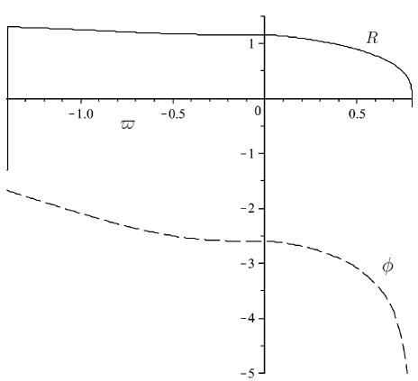
Figure 1: The real parts of scale factor (full curve) and scalar field (broken curve) in the first life with respect to $\varpi$ for $\lambda=0.27,\beta=-0.45$.

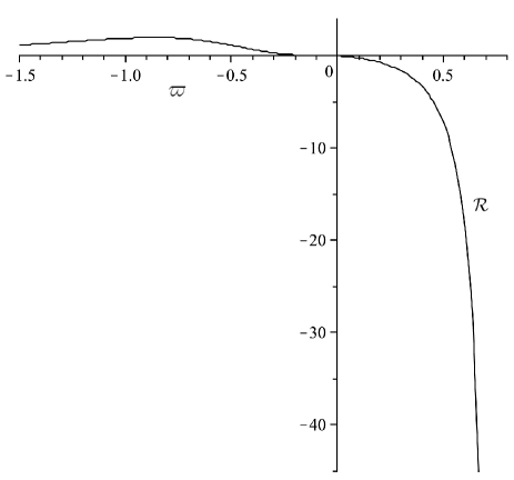
Figure 2: The behavior of Ricci scalar with respect to $\varpi$ for $\lambda=0.27,\beta=-0.45$.

6 Quantum Cosmology

The high energy and small scale of very early universe provides the possibility of having noncommutativity and GUP in the minisuperspace configurations of the model discussed here. But, in such small scale the quantum behavior is inevitable. Thus, it is necessary to study the quantized model and check if the quantization results are consistent with the classical solutions of dynamical equations.

Introducing the momentum quantum operators $\hat{p_{1}}=-i\partial/\partial x_{1},\,\hat{p_{2}}=-i\partial/\partial x_{2}$ and applying the Weyl symmetrization rule to (36) to construct the Hamiltonian operator, leads to the Wheeler-DeWitt(WD) equation of the form $\hat{{\cal H}}^{\prime}\Psi(x_{1},x_{2})=0$. Defining the real and imaginary parts of the wave function as $\Psi=\psi_{r}+i\psi_{i}$ splits WD equation in to two parts

$$H_{1}\psi_{r}-H_{2}\psi_{i}=0,\hskip 28.45274ptH_{2}\psi_{r}+H_{1}\psi_{i}=0,$$ (46)

where,

$$H_{1}=8a_{1}\beta(x_{1}-x_{2})(\partial_{1}+\partial_{2})+a_{1}(x_{1}^{2}-x_{2}^{2})\left[2\beta(\partial_{1}+\partial_{2})^{2}-1\right]-\frac{1}{4}(\partial_{1}^{2}-\partial_{2}^{2}),$$

$$H_{2}=8a_{1}\beta(x_{1}\partial_{1}-x_{2}\partial_{2}).$$ (47)

In order to obtain a quantum criterion to test the classical results of previous section, we consider the special case $\psi_{r}={\cal A}\psi_{i}\equiv F(x_{1},x_{2})$, ${\cal A}$ being a constant. This converts (46) into $H_{1}F=0$ and $\,H_{2}F=0$, the second of which is automatically satisfied if $F=F(x_{1}x_{2})$, and the first one becomes

$$\left(2a_{1}\beta(x_{1}^{2}+X)^{2}+\frac{1}{4}x_{1}^{2}\right)\frac{d^{2}F}{dX^{2}}+12a_{1}\beta\,x_{1}^{2}\,\frac{dF}{dX}-a_{1}\,x_{1}^{2}\,F=0,$$ (48)

where $X:=x_{1}x_{2}$ and $x_{1}$ is regarded as a parameter. The solution of (48) is an expression of Generalized Hypergeometric Functions as

$$F(x_{1},x_{2})=A_{1}\,\,{}_{2}\mathrm{F}_{1}\left(D_{+}(x_{1}),D_{-}(x_{1})\,;\,-S^{\prime}(x_{1})\,;\,\frac{1}{2}-a_{1}\beta S(x_{1})\left(1+\frac{x_{2}}{x_{1}}\right)\right)+$$

$$A_{2}\,h(x_{1},x_{2})\,\,_{2}\mathrm{F}_{1}\left(S^{\prime}(x_{1})-D_{-}(x_{1}),S^{\prime}(x_{1})-D_{+}(x_{1})\,;\,S^{\prime}(x_{1})+2\,;\,\frac{1}{2}-a_{1}\beta S(x_{1})\left(1+\frac{x_{2}}{x_{1}}\right)\right),$$

where $A_{1},A_{2}$ are two constants and

$$h(x_{1},x_{2})=x_{1}^{2}\left(2\sqrt{-2a_{1}\beta}(x_{1}+x_{2})-1\right)^{S^{\prime}(x_{1})+S(x_{1})}.$$ (50)

As figure 3 shows, the density plot of the quantum solution (50) is in good agreement with the classical solution obtained in the previous section.

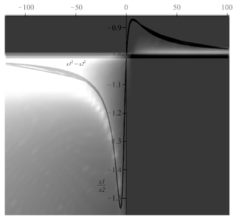
Figure 3: Density plot of $|\Psi|^{2}$ for $\lambda=0.27,\beta=-0.45$ which is in good agreement with the superimposed classical path.

7 Conclusions

Using a noncommutative phase space of dynamical variables deformed by Generalized Uncertainty Principle we have shown that continuous signature transition from Euclidean to Lorentzian may occurs for a model described by FRW metric minimally coupled with a free massless scalar field $\phi$ accompanied by a cosmological constant. The transformations of GUP in deforming the phase space breaks the symmetry of Hamiltonian under $\phi\rightarrow-\phi$ causing a possible continuous change of signature. This indicates that for a signature transition to happen, instead of a massive scalar field having an ad hoc and complicate potential, we just need a free massless scalar field, a cosmological constant and a noncommutative phase space deformed by GUP. These elements are supposed to be trivial in the extreme conditions at early universe. In commutative [36] as well as moyal transformed noncommutative Hamiltonian [51], we need a coupling $b$ in the scalar field potential to trigger the signature transition. However, using GUP in the absence of such potential and coupling, we have the expression $\beta^{\prime}p_{1}p_{2}$ in Hamiltonian (36) coming directly from the special structure of GUP deformations (34) which means that the GUP noncommutativity can cause a change of signature by itself. In other words, GUP accompanied by noncommutativity may establish a general framework for a continuous change of signature. Moreover, in principle, the signature transition is possible for both negative and positive cosmological constants. This significantly differs from the moyal approach [51] in which only the negative values of cosmological constant are acceptable. We have also studied the quantum cosmology of this model and obtained a solution of Wheeler-DeWitt equation showing a good correspondence with the classical path.

References

- [1] E. Wigner, Phys. Rev. 40 (1932) 749.
- [2] H. S. Snyder, Phys. Rev. 71 (1947) 38.
- [3] A. Connes, Inst. Hautes Etudes Sci. Publ. Math. 62 (1985) 257.
- [4] S. L. Woronowicz, Pub. Res. Inst. Math. Sci. 23 (1987) 117.
- [5] M. Maceda, J. Madore, P. Manousselis, and G. Zoupanos, Eur. Phys. J. C 36 (2004) 529.
- [6] N. Seiberg and E. Witten, JHEP 9909 (1999) 032.
- [7] J. E. Moyal: Proceedings of the Cambridge philosophical society 45 (1949) 99.
- [8] D. J. Gross and P. F. Mendle, Nucl. Phys. B 303, (1988) 407.
- [9] D. J. Gross, Phys. Rev. Lett. 60 (1988) 1229.
- [10] D. Amati, M. Ciafaloni and G. Veneziano, Phys. Lett. B 216 (1989) 41.
- [11] M. Kato, Phys. Lett. B 245 (1990) 43.
- [12] K. Konishi, G. Paffuti and P. Provero, Phys. Lett. B 234 (1990) 276.
- [13] L. G. Garay, Int. J. Mod. Phys. A 10 (1995) 145.
- [14] S. Haro, J. High Energy Phys. JHEP 10 (1998) 023.
- [15] E. Witten, Phys. Today 49 (1996) 24.
- [16] G. Amelino-Camelia, N. E. Mavromatos, J. Ellis and D. V. Nanopoulos, Mod. Phys. Lett. A 12 (1997) 2029.
- [17] G.Veneziano, Europhys.Lett.2 (1986) 199.
- [18] M. Maggiore, Phys. Lett. B 304 (1993) 65.
- [19] D. J. Gross and P. F. Mende, Phys. Lett. B 197 (1987) 129.
- [20] M.Maggiore, Phys. Lett. B 319 (1993) 83.
- [21] M. Maggiore, Phys. Rev. D 49 (1994) 5182.
- [22] S. Capozziello, G. Lambiase and G. Scarpetta [arXiv:gr-qc/9910017].
- [23] D. V. Ahluwalia, Phys. Lett. A 275 (2000) 31.
- [24] D. V. Ahluwalia, Mod. Phys. Lett. A 17 (2002) 1135.
- [25] G. Amelino-Camelia, Int. J. Mod. Phys. D 11 (2002) 35.
- [26] J. Magueijo and L. Smolin, Phys. Rev. Lett. 88 (2002) 190403.
- [27] J. Magueijo and L. Smolin, Phys. Rev. D 71 (2005) 026010.
- [28] J. L. Cortes, J. Gamboa, Phys. Rev. D 71 (2005) 065015 .
- [29] A. Kempf, G. Mangano and R. B. Mann, Phys. Rev. D 52 (1995) 1108.
- [30] A. Kempf and G. Mangano, Phys. Rev. D 55 (1997) 7909.
- [31] R. J. Adler and D. I. Santiago, Mod. Phys. Lett. A 14 (1999) 1371.
- [32] F. Scardigli, Phys. Lett. B 452 (1999) 39.
- [33] W. Chagas-Filho [arXiv:hep-th/0505183].
- [34] J. Y. Bang and M. S. Berger, Phys. Rev. D 74 (2006) 125012.
- [35] J. B. Hartle and S. W. Hawking, Phys. Rev. D 28 (1983) 2960.
- [36] T. Dereli and R. W. Tucker, Class. Quant. Grav. 10 (1993) 365.
- [37] A. C. Hirshfeld and P. Henselder, Am. J. Phys. 70 (2002) 537.
- [38] M. Chaichian, M. M. Sheikh-Jabbari, A. Tureanu, Phys. Rev. Lett. 86 (2001) 2716.
- [39] M. Chaichian, A. Tureanu, R. B. Zhang, X. Zhang, J. Math. Phys. 49 (2008) 073511.
- [40] Y.-F. Cai and Y.-S. Piao, Phys. Lett. B 657, (2007) 1.
- [41] Y.-F. Cai and Y. Wang, JCAP 0706, (2007) 022; Y.-F. Cai and Y. Wang, JCAP 0801, (2008) 001.
- [42] P. A. M. Dirac, Lectures on quantum mechanics, (Yeshiva University, Academic-Press, New York, 1997).
- [43] R. Arnowitt, S. Deser, and C. W. Misner, in Gravitation: an introduction to current research (Wiley, New York, 1962).
- [44] F. Darabi and H. R. Sepangi, Class. Quant. Grav. 16 (1999) 1565.
- [45] F. Darabi, Phys. Lett. A 259 (1999) 97.
- [46] F. Darabi, A. Rastkar, Gen. Rel. Grav. 38 (2006) 1355.
- [47] K. Ghafoori, S. S. Gusheh and H. R. Sepangi, Int. J. Mod. Phys. A 15 (2000) 1521.
- [48] T. Dereli, M. Önder and R. W. Tucker, Class. Quant. Grav. 10 (1993) 1425.
- [49] B. Vakili, S. Jalalzadeh and H. R. Sepangi, JCAP 0505 (2005) 006.
- [50] S. Jalalzadeh, F. Ahmadi and H. R. Sepangi, JHEP 0308 (2003) 012.
- [51] T. Ghaneh, F. Darabi and H. Motavalli, Mod. Phys. Lett. A 27, (2012) 1250214.
- [52] L. Nam Chang, D. Minic, N. Okamura and T. Takeuchi, Phys. Rev. D 65 (2002) 125028.
- [53] A. Kempf, J. Phys. A 30 (1997) 2093.
- [54] L. Nam Chang, D. Minic, N. Okamura and T. Takeuchi, Phys. Rev. D 65 (2002) 125027.
- [55] B. Vakili, H. R. Sepangi, Phys. Lett. B 651 (2007) 79.
- [56] S. Das and E. C. Vagenas, Phys. Rev. Lett. 101 (2008) 221301.
- [57] B. Vakili, Phys. Rev. D 77 (2008) 044023.
- [58] H. R. Sepangi, B. Shakerin and B. Vakili, Class. Quant. Grav. 26 (2009) 065003.