Pseudo-Critical Temperature and Thermal Equation of State from $N_{f}=2$ Twisted Mass Lattice QCD

Abstract:

We report about the current status of our ongoing study of the chiral limit of two-flavor QCD at finite temperature with twisted mass quarks. We estimate the pseudo-critical temperature $T_{c}$ for three values of the pion mass in the range of $m_{\mathrm{PS}}\simeq 300$ and $500\mathrm{~{}MeV}$ and discuss different chiral scenarios.

Furthermore, we present first preliminary results for the trace anomaly, pressure and energy density. We have studied several discretizations of Euclidean time up to $N_{\tau}=12$ in order to assess the continuum limit of the trace anomaly. From its interpolation we evaluate the pressure and energy density employing the integral method. Here, we have focussed on two pion masses with $m_{\mathrm{PS}}\simeq 400$ and $700\mathrm{~{}MeV}$.

1 Introduction

The order of the phase transition in the case of two-flavor QCD in the chiral limit remains an open question. While with Wilson quarks [1, 2] the transition is found to be compatible with a second order phase transition in the universality class of a 3d $O(4)$ spin model, a first order transition seems to be favoured in analyses with staggered fermions at $N_{\tau}=4$ [3, 4].

The thermal equation of state (EoS) constitutes a relevant ingredient in the hydrodynamic evolution of the quark-gluon plasma created in heavy-ion experiments. It can be determined non-perturbatively in lattice calculations. In the recent past the EoS has been studied extensively using the staggered type of quark discretization, mostly with $N_{f}=2+1$ flavors at the physical point [5, 6]. The much more compute-intensive Wilson-like discretizations are less investigated however [7, 8]. In the latter study the fixed scale approach is used as compared to the more traditional fixed $N_{\tau}$ approach.

2 Lattice Setup

The lattice setup in our ongoing investigations equals the one employed by the European Twisted Mass Collaboration (ETMC) for their $N_{f}=2$ simulations [9]. It employs the twisted mass action in terms of the twisted fields $\chi=\exp{(-i\pi\gamma_{5}\tau_{3}/4)}\psi$

$$S^{\mathrm{tm}}_{f}[U,\psi,\bar{\psi}]=\sum_{x,y}\bar{\chi}(x)\left(\delta_{x,y}-\kappa D_{\mathrm{W}}(x,y)[U]+2i\kappa a\mu\gamma_{5}\tau_{3}\delta_{x,y}\right)\chi(y)\;.$$ (1)

in the quark sector, while the gauge sector is described by the tree-level Symanzik improved gauge action

$$S_{g}^{\mathrm{tlSym}}[U]=\beta\Big{(}c_{0}\sum_{P}[1-\frac{1}{3}\mathrm{Re}\mathrm{Tr}\left(U_{P}\right)]+c_{1}\sum_{R}[1-\frac{1}{3}\mathrm{Re}\mathrm{Tr}\left(U_{R}\right)]\Big{)}\;.$$ (2)

The latter two sums extend over all possible plaquettes ($P$) and all possible planar rectangles ($R$), respectively.

3 Pseudo-Critical Temperatures and Chiral Limit

For the present study of the chiral limit we rely on simulations with $N_{\tau}=12$ at pion masses $m_{\mathrm{PS}}\simeq 320~{}\mathrm{MeV}$, $400~{}\mathrm{MeV}$ and $470~{}\mathrm{MeV}$ that have been analyzed in Ref. [10] (for historical reasons we call these ensembles A12, B12 and C12). Our determination of the pseudo-critical temperature is based on the measurement of the variance of $\bar{\psi}\psi$ over the gauge ensemble

$$\sigma^{2}_{\bar{\psi}\psi}=\frac{V}{T}\left(\left<(\bar{\psi}\psi)^{2}\right>-\left<\bar{\psi}\psi\right>^{2}\right)\;.$$ (3)

It corresponds to the disconnected part of the usual chiral susceptibility and should show a maximum in the region of $T_{c}$. This is indeed the case for all our ensembles and two representative cases are shown in the two left panels of Fig. 1. From fitting Gaussian function to the data of $\sigma^{2}_{\bar{\psi}\psi}$ around the maxima we infer values of the pseudo-critical couplings $\beta_{c}$ that are converted to a physical value of $T_{c}$ using an interpolation of $a(\beta)$ [10]. At leading order in chiral perturbation theory and for a phase transition of second order the pion mass dependence of $T_{c}$ is expected to be given as

$$T_{c}(m_{\pi})=T_{c}(0)+A\ m_{\pi}^{2/(\tilde{\beta}\delta)}\;,$$ (4)

where $T_{c}(0)$ is the critical temperature in the chiral limit and $\tilde{\beta}$ and $\delta$ are critical exponents corresponding to the universality class of second order phase transition. We have restricted ourselves to the chiral scenarios discussed in Ref. [10] including a first order scenario as well as the $O(4)$ and $Z(2)$ second order scenarios, for the latter assuming a second order endpoint located at $m_{\pi,c}=0~{}\mathrm{MeV}$ or alternatively at $m_{\pi,c}=200~{}\mathrm{MeV}$. The result of fits of Eq. (4) to our data is shown in the right most panel of Fig. 1. As the fitted curves are all describing the given data quite well we conclude that the present set of pion mass values can not discriminate among the different chiral scenarios that have been studied. For the $O(4)$ model the fit prefers a value of $T_{c}(0)=152~{}(26)\mathrm{~{}MeV}$.

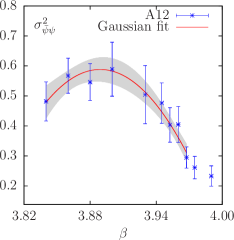
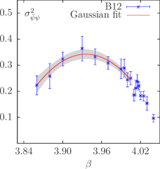
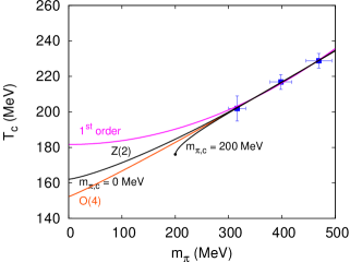
Figure 1: Determination of $T_{c}$ from $\sigma^{2}_{\bar{\psi}\psi}$ using a Gaussian fit to the maximum for the A12 and B12 ensembles. Comparison of different scenarios for the chiral limit of $T_{c}$.

4 The Trace Anomaly

For the EoS we concentrate on one of the values of pion masses used in the chiral limit study above, namely the one corresponding to $m_{\mathrm{PS}}\simeq 400~{}\mathrm{MeV}$. We have added at the same pion mass additional runs at smaller $N_{\tau}=4,~{}6\mathrm{~{}and~{}}8$ (henceforth denoted by B4, B6, B8 $\ldots$). Apart from the latter, for which $N_{\sigma}=28$ has been chosen, all lattices have a spatial extent $N_{\sigma}=32$. Moreover, further ensembles at $m_{\mathrm{PS}}\simeq 700~{}\mathrm{MeV}$ (further on referred to as the D mass) were generated with sizes $N_{\sigma}^{3}\times N_{\tau}=24^{3}\times 10,~{}20^{3}\times 8\mathrm{~{}and~{}}16^{3}\times 6$ (referred to as D10, D8 and D6).

The direct evaluation of pressure $p=T\left.\frac{\partial\ln Z}{\partial V}\right|_{T}$ and energy density $\epsilon=\left.\frac{T}{V}\frac{\partial\ln Z}{\partial\ln T}\right|_{V}$ from derivatives of the partition function $Z$ is problematic given the lattice spacing dependence of both the temperature $T=1/(N_{\tau}a)$ and the volume $V=N_{\sigma}^{3}a^{3}$. The by now standard approach is the use of the integral method to calculate the pressure as a temperature integral of the total derivative of the partition function with respect to the lattice spacing, the so called trace anomaly:

$$\begin{split}\frac{I}{T^{4}}&=\frac{\epsilon-3p}{T^{4}}=-\frac{T}{VT^{4}}\left<\frac{d\ln Z}{d\ln a}\right>_{\mathrm{sub}}\\ &=N_{\tau}^{4}B_{\beta}\frac{1}{N_{\sigma}^{3}N_{\tau}}\Bigg{\{}\frac{c_{0}}{3}\left<\mathrm{Re}\mathrm{Tr}\sum_{P}U_{P}\right>_{\mathrm{sub}}+\frac{c_{1}}{3}\left<\mathrm{Re}\mathrm{Tr}\sum_{R}U_{R}\right>_{\mathrm{sub}}+B_{\kappa}\left<\bar{\chi}D_{\mathrm{W}}[U]\chi\right>_{\mathrm{sub}}\\ &\hphantom{N_{\tau}^{4}B_{\beta}\frac{1}{N_{\sigma}^{3}N_{\tau}}\Bigg{\{}}-\left[2(a\mu)B_{\kappa}+2\kappa_{c}(a\mu)B_{\mu}\right]\left<\bar{\chi}i\gamma_{5}\tau^{3}\chi\right>_{\mathrm{sub}}\Bigg{\}}\;.\end{split}$$ (5)

Here, $B_{\beta}$, $B_{\mu}$ and $B_{\kappa}$ are related to the $\beta$-functions, the derivatives of the bare parameters with respect to the lattice spacing, as follows:

$$B_{\beta}=a\frac{d\beta}{da}\;,\quad\quad B_{\mu}=\frac{1}{(a\mu)}\frac{\partial(a\mu)}{\partial\beta}\;,\quad\quad B_{\kappa}=\frac{\partial{\kappa_{c}}}{\partial{\beta}}\;.$$ (6)

It is necessary to subtract from each term in above expression the corresponding $T=0$ vacuum contribution $\left<\ldots\right>_{\mathrm{sub}}\equiv\left<\ldots\right>_{T>0}-\left<\ldots\right>_{T=0}$ in order to achieve a finite result. Details of the subtraction on the basis of the available $T=0$ lattice data as well as on the evaluation of the $\beta$-functions will be given in the following section. In the left panels of Figs. 3 and 4 we show the trace anomaly for the two cases of pseudoscalar masses under investigation. In both cases we observe sizeable lattice artifacts in the height of the maximum and even in the falling edge at larger temperatures. Moreover, the precision in case of the smaller mass is not yet satisfactory, especially at small temperatures.

5 $\beta$-Functions and $T=0$ Subtraction

For evaluating the three $\beta$-functions we consider fits to lattice data of the Sommer scale $r_{0}$ in the chiral limit (denoted by $\left(\frac{r_{\chi}}{a}\right)$). To this end the correct asymptotic behavior is built into the fit functions explicitly following Ref. [11]. For instance we determine $B_{\beta}$ via the identity

$$B_{\beta}=\left(a\frac{d\beta}{da}\right)=-\left(\frac{r_{\chi}}{a}\right)\left(\frac{d\left(\frac{r_{\chi}}{a}\right)}{d\beta}\right)^{-1}\;,$$ (7)

by fitting $r_{\chi}/a$ to the formula

$$\left(\frac{r_{\chi}}{a}\right)(\beta)=\frac{1+n_{0}R(\beta)^{2}}{d_{0}\left(a_{\mathrm{2L}}(\beta)+d_{1}R(\beta)^{2}\right)},\quad\quad R(\beta)=\frac{a_{\mathrm{2L}}(\beta)}{a_{\mathrm{2L}}(\beta_{\mathrm{sub}})}\;.$$ (8)

The ratio $R(\beta)$ is defined in terms of the known two-loop perturbative formula $a_{\mathrm{2L}}(\beta)$ and $\beta_{\mathrm{sub}}=3.9$ has been chosen in above formula. The three parameter fit of Eq. (8) to $\left(\frac{r_{\chi}}{a}\right)$ (see the left panel of Fig. 2) yields $\chi^{2}/\mathrm{dof}=1.2$. The thus obtained $\beta$-function is shown in the middle panel of Fig. 2. The interpolation provided by the fit of Eq. (8) has also been used to set the scale using the physical value of $r_{0}=0.420(15)\mathrm{~{}fm}$ by ETMC [12].

The second $\beta$-function associated with the mass is evaluated from a similar identity [11]:

$$B_{\mu}=\frac{1}{(a\mu)}\frac{\partial(a\mu)}{\partial\beta}=B^{-1}_{\beta}+\frac{1}{r_{\chi}\mu}\frac{\partial(r_{\chi}\mu)}{\partial\beta}\;.\\$$ (9)

$r_{\chi}\mu$ as well as its derivative are obtained by fitting the following expression to $r_{\chi}\mu$:

$$r_{\chi}\mu=\left(\frac{12\beta_{0}}{\beta}\right)^{\gamma_{0}/2\beta_{0}}P(\beta),\quad\quad P(\beta)=a_{\mu}\left(1+b_{\mu}R(\beta)^{2}\right)\;,$$ (10)

where $\beta_{0}=(11-2N_{f}/3)/(4\pi)^{2}$ and $\gamma_{0}=1/(2\pi^{2})$. The third and remaining $\beta$-function involving $B_{\kappa}$ is calculated in the most straight-forward manner from an explicit derivative of $\kappa_{c}$ with respect to $\beta$ using the Padé interpolation of Ref. [13].

In order to obtain $\left<\ldots\right>_{\mathrm{sub}}$, i. e. to subtract the $T=0$ expectation values, we have used all available lattice data from ETMC. For these it has been necessary to interpolate in $a\mu$ using spline functions to match with the simulated bare mass at $T>0$. Further additional $T=0$ runs have been simulated in order to perform the subtraction more reliably. However, not all simulation points at finite temperature are supplemented with an associated $T=0$ simulation. Thus, we have performed an interpolation in $\beta$ using a polynomial ansatz of fifth order. For the plaquette, the rectangle and the Wilson hopping term $D_{\mathrm{W}}$ we have obtained values for $\chi^{2}$ per degree of freedom of $2.7$, $2.3$ and $2.9$, respectively. The remaining term, for which no fit of reasonable quality could be obtained using this ansatz, has been interpolated using splines. For the D ensembles with larger mass, sufficient $T=0$ data newly generated is available. Hence, no interpolations in the bare coupling and only few interpolations in the bare mass had to be done.

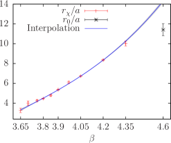
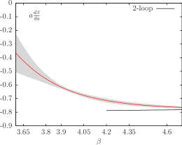
Figure 2: Left: Interpolation of $r_{\chi}/a$ in the bare coupling. The point at $\beta=4.6$ is not obtained from a chiral extrapolation and is not included in the fit. Middle: The $\beta$-function obtained according to Eq. (7). We also show the perturbative 2-loop expectation at large couplings $B_{\beta}\left(\beta\right)=-12\beta_{0}-72\frac{\beta_{1}}{\beta}$. Right: Pion mass in physical units for the B ensembles together with a constant fit over all data points.

6 Pressure and Energy Density

The evaluation of the pressure from the integral technique proceeds by integrating the identity $\frac{I}{T^{4}}=T\frac{\partial}{\partial T}\left(\frac{p}{T^{4}}\right)$ in temperature along the line of constant physics (LCP):

$$\frac{p}{T^{4}}-\frac{p_{0}}{T_{0}^{4}}=\left.\int_{T_{0}}^{T}d\tau\frac{\epsilon-3p}{\tau^{5}}\right|_{\mathrm{LCP}}\;.$$ (11)

We define the LCP in terms of the pion mass in physical units, which for the smaller mass run is shown in the right panel of Fig. 2. As can be seen it is constant within errors. For the larger mass, however, we observe a systematic rise of $m_{\mathrm{PS}}$ towards larger coupling which amounts to a violation of the LCP condition on the level of $10\%$.

We perform the integration Eq. (11) by fitting the available lattice data of $\frac{I}{T^{4}}$ to the ansatz [6]

$$\frac{I}{T^{4}}=\exp{\left(-h_{1}\bar{t}-h_{2}{\bar{t}}^{2}\right)}\cdot\left(h_{0}+\frac{f_{0}\left\{\tanh{\left(f_{1}\bar{t}+f_{2}\right)}\right\}}{1+g_{1}\bar{t}+g_{2}{\bar{t}}^{2}}\right)\;,$$ (12)

where $\bar{t}=T/T_{0}$ and $T_{0}$ is a free parameter in the fit. For the fit we use the tree-level corrected data of the trace anomaly that we obtain by normalizing it with the lattice-to-continuum ratio of the Stefan-Boltzmann pressure in the free limit $p_{\mathrm{SB}}^{L}/p_{\mathrm{SB}}$ following Ref. [6]. We check the validity of this approach by comparing the continuum limit values as obtained from the corrected as well as uncorrected data for various temperatures and find compatible results in the majority of cases. As can be observed from Figs. 3 and 4, where the thus corrected trace anomaly is shown for the various available $N_{\tau}$, the correction is efficient and overlays the data from different $N_{\tau}$.

In order to account for the large errors at small temperatures we perform fits of Eq. (12) to the upper and lower 1-$\sigma$ deviations and keep the resulting difference as the error of the interpolation. For the B (D) ensembles we have fitted data from $N_{\tau}=8,10$ and $12$ ($N_{\tau}=8$ and $10$) simultaneously and obtain acceptable fits in both cases. We subsequently integrate the interpolation curve numerically in temperature. The integration constant $p_{0}$ in Eq. (11) has been set to zero in the present evaluation. The (yet preliminary) results for the pressure and energy density are shown in the right panels of Figs. 4 and 3.

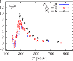
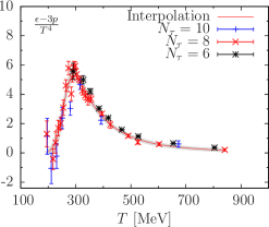
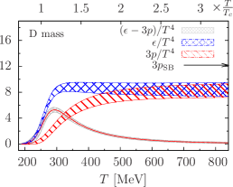
Figure 3: Left: The trace anomaly for the D ensembles (see text) obtained for different values of the temporal extent $N_{\tau}$. Middle: The trace anomaly after tree-level correction with a fit of Eq. (12). Right: Preliminary results for the pressure and the energy density.

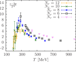
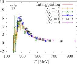
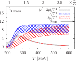
Figure 4: The same as in Fig. 3 but for the B ensembles (see text).

7 Conclusions

We have presented results for the mass dependence of the pseudo-critical temperature for several small values of the pion mass in the range of $m_{\mathrm{PS}}\simeq 320~{}\mathrm{MeV}$ and $m_{\mathrm{PS}}\simeq 470~{}\mathrm{MeV}$ in a setup with $N_{f}=2$ Wilson twisted mass quarks at $N_{\tau}=12$. The comparison of different scenarios in the chiral limit is so far inconclusive at the present masses. Further, we have presented first, yet preliminary, results of our ongoing project aiming at the determination of the EoS. The trace anomaly has been computed for two values of the pseudoscalar mass of about $400$ and $700\mathrm{~{}MeV}$ and has been tree-level corrected. The pressure has been calculated from the integral method using a smooth interpolation formula fitted to the corrected trace anomaly.

References

- [1] CP-PACS Collaboration, A. Ali Khan et al., Phys.Rev. D63 (2001) 034502, arXiv:[hep-lat/0008011].
- [2] V. Bornyakov et al., Phys.Rev. D82 (2010) 014504, arXiv:0910.2392 [hep-lat].
- [3] C. Bonati et al., Nucl.Phys. A820 (2009) 243C–246C.
- [4] C. Bonati et al., PoS LATTICE2011 (2011) 189, arXiv:1201.2769 [hep-lat].
- [5] M. Cheng et al., Phys. Rev. D81 (2010) 054504, arXiv:0911.2215 [hep-lat].
- [6] S. Borsanyi et al., JHEP 1011 (2010) 077, arXiv:1007.2580 [hep-lat].
- [7] CP-PACS Collaboration, A. Ali Khan et al., Phys.Rev. D64 (2001) 074510, arXiv:[hep-lat/0103028].
-
[8]
WHOT-QCD Collaboration, T. Umeda et al.,
Phys.Rev.
D85 (2012) 094508,
arXiv:1202.4719 [hep-lat]. - [9] ETM Collaboration, P. Boucaud et al., Comput. Phys. Commun. 179 (2008) 695, arXiv:0803.0224 [hep-lat].
- [10] tmfT Collaboration F. Burger et al., Revised version of arXiv:1102.4530 [hep-lat].
- [11] M. Cheng et al., Phys.Rev. D77 (2008) 014511, arXiv:0710.0354 [hep-lat].
- [12] ETM Collaboration, R. Baron et al., JHEP 1008 (2010) 097, arXiv:0911.5061 [hep-lat].
-
[13]
tmfT Collaboration, F. Burger et al.,
PoS LATTICE2010 (2010) 220,
arXiv:1009.3758 [hep-lat]. - [14] O. Philipsen and L. Zeidlewicz, Phys.Rev. D81 (2010) 077501, arXiv:0812.1177 [hep-lat].