A Conformal Approach for Surface Inpainting
Abstract.
We address the problem of surface inpainting, which aims to fill in holes or missing regions on a Riemann surface based on its surface geometry. In practical situation, surfaces obtained from range scanners often have holes or missing regions where the 3D models are incomplete. In order to analyze the 3D shapes effectively, restoring the incomplete shape by filling in the surface holes is necessary. In this paper, we propose a novel conformal approach to inpaint surface holes on a Riemann surface based on its surface geometry. The basic idea is to represent the Riemann surface using its conformal factor and mean curvature. According to Riemann surface theory, a Riemann surface can be uniquely determined by its conformal factor and mean curvature up to a rigid motion. Given a Riemann surface , its mean curvature and conformal factor can be computed easily through its conformal parameterization. Conversely, given and , a Riemann surface can be uniquely reconstructed by solving the Gauss-Codazzi equation on the conformal parameter domain. Hence, the conformal factor and the mean curvature are two geometric quantities fully describing the surface. With this - representation of the surface, the problem of surface inpainting can be reduced to the problem of image inpainting of and on the conformal parameter domain. The inpainting of and can be done by conventional image inpainting models. Once and are inpainted, a Riemann surface can be reconstructed which effectively restores the 3D surface with missing holes. Since the inpainting model is based on the geometric quantities and , the restored surface follows the surface geometric pattern as much as possible. We test the proposed algorithm on synthetic data, 3D human face data and MRI-derived brain surfaces. Experimental results show that our proposed method is an effective surface inpainting algorithm to fill in surface holes on an incomplete 3D models based their surface geometry.
Key words and phrases:
Surface inpainting, conformal parameterization, conformal factor, mean curvature, Gauss-Codazzi equation1991 Mathematics Subject Classification:
Primary: 53B20, 30L10, 53C21 Secondary: 53B21, 92-08.1. Introduction
Surface processing is an important topic in computer graphics, computer visions and medical imaging. Examples includes surface denoising, surface inpainting, surface remeshing and so on. Amongst the various tasks in surface processing, the problem of surface inpainting, which aims to fill in holes or missing regions on a Riemann surface, is an important pre-processing step necessary for the geometric analysis of incomplete 3D shapes. Digital 3D surfaces containing holes are common. In practical situation, real-life objects are usually captured from range scanners. Despite the recent advance in the laser scanning technology, 3D models obtained from even the most sophisticated acquisition devices are often incomplete due to occlusions, low reflectance, constraints during recording or self-occlusions of complicated geometry. This results in holes or missing regions in the obtained 3D digital models. In order to analyze the geometric objects effectively or derive a visually appealing 3D models, developing an effective algorithm for filling in holes or missing regions on a surface is of utmost importance.
In this paper, we propose a framework for filling in holes or missing regions on a Riemann surface using conformal geometry. The ultimate goal is to obtain a restored surface with holes filled based on the surface geometry, so that the basic geometry of the surface can be smoothly patched. For this purpose, a good representation of the Riemann surface describing its geometry is required. In this work, we propose to represent the Riemann surface using its conformal factor and mean curvature. According to Riemann surface theory, a Riemann surface can be uniquely determined by its conformal factor and mean curvature up to a rigid motion. Given a Riemann surface , its mean curvature and conformal factor can be computed easily through its conformal parameterization. Conversely, given and , a Riemann surface can be uniquely reconstructed by solving the Gauss-Codazzi equation on the conformal parameter domain. Hence, the conformal factor and the mean curvature are two geometric quantities fully describing the surface. Given the - representation of an incomplete surface, the problem of surface inpainting can be reformulated into the image inpainting problem of and . Using the conventional image inpainting techniques, both and can be inpainted on the conformal parameter domain. A Riemann surface can then be reconstructed which restores the 3D surface with missing holes. Since the proposed inpainting model is based on two geometric quantities fully determining the surface, the surface holes can be effectively filled , which follows the surface geometric pattern. We test the proposed algorithm on synthetic data, 3D human face data and MRI-derived brain surfaces. Experimental results show that our algorithm can effectively inpaint surface holes based on the surface geometry to restore the incomplete 3D surface models.
The contributions of this paper are two-folded. First, we consider the representation of a Riemann surface using its conformal factor and mean curvature . Given two scalar functions and , the associated Riemann surface can be reconstructed through solving the Gauss-Codazzi equation numerically. Second, we propose a surface inpainting algorithm by inpainting the scalar functions and . The surface inpainting algorithm is based on and , which are two geometric quantities fully describing the surface. Hence, the proposed surface inpainting algorithm can fill in surface holes based on the surface geometry.
Our paper is organized as follows: prior work on related topics is presented in section 2. The basic mathematical theory is discussed in section 3. In Section 4, the details of our proposed surface representation using conformal factor and mean curvature are discussed. The detailed algorithm for surface inpainting is described in Section 5. In Section 6, the numerical algorithms are summarized. Experimental results are reported in Section 7, and some conclusions and future work are discussed in Section 8.
2. Previous work
In this section, we will review some relevant works closely related to our paper.
The problem of surface inpainting was inspired by 2D image completion, which has been widely studied by different groups. Different variational models have been proposed [1, 2, 4, 5, 6]. The basic idea is to diffuse the image intensity into the inpainting domain from its surrounding regions based on various regularizations of the solution. For example, Chan et al. [1, 2] proposed the total variation (TV) models for image inpainting. Euler elastica model [4, 5, 6] has also been proposed, which is essentially a variational model with a regularizing term containing higher-order derivatives. Other examples include the active contour model based on Mumford and Shahs segmentation [10], the inpainting scheme based on the Mumford-Shah-Euler image model [3], the inpainting model with the Navier-Stokes equation [7], and wavelet-based inpainting algorithms [8, 9]. For a detailed introduction to image inpainting, we refer the readers to [4].
3D surface processing has also been extensively studied. Different surface denoising algorithms have been proposed. For example, surface smoothing by mean curvature flow or Laplace smoothing have been proposed [11, 12, 13], which are effective for removing oscillations on noisy surfaces. In order to preserve ridges and sharp corners of the surfaces, different second order anisotropic surface diffusion models have been considered [14, 15, 16, 17], which minimizes the weighted surface area. Higher-order isotropic or anisotropic flows based on minimizing the surface total curvature or weighted total curvature have also been discussed [18, 19]. Besides, various surface inpainting algorithms to fill in surface holes have been proposed [20, 23, 22, 24, 25, 21]. A common approach is to fill in the occluded regions with surface patches, which smoothly attach to the boundary vertices of the surface holes [23, 22]. For example, Clarenz et al. [23] proposed to fill in surface holes by minimizing the Willmore energy functional. The surface patches obtained is guaranteed to satisfy the continuity properties. Davis et al. [22] proposed to extend a signed distance function, which is initially defined only on domains close to the known surface, to the complete space using volumetric diffusion. The surface can then be completed, even for non-trivial hole boundaries. Later, Caselles et al. [20] proposed a level set variational framework based on the minimization of the norm of the mean curvature for surface inpainting. The algorithm produces an inpainted surface with minimal surface area given the boundary constraints, although the restored surface may produce non-smooth global geometry. Most of the above algorithms do not incorporate or only partially incorporate the geometric information of the surface into their models. The inpainting result obtained usually does not follow surface geometric pattern, and thus the restored surface might often be unnatural. In this paper, we propose to inpaint surface holes through inpainting the conformal factor and mean curvature, which are two geometric quantities fully determining the surface. The inpainted surface can better follow the surface geometric pattern.
The proposed surface inpainting model in this paper is based on the conformal structure of the Riemann surface. The problem of computing the conformal structure of a Riemann surface has been extensively studied, and different algorithms have been proposed [27, 28, 30, 35, 26, 29]. For example, Hurdal et al. [26] proposed to compute the conformal parameterization using circle packing and applied it to the registration of human brains. Gu et al. [28, 30, 29] proposed to compute the conformal parameterizations of human brain surfaces for registration using harmonic energy minimization and holomorphic 1-forms. Using conformal factor and curvatures, a shape index has also been proposed to measure geometric difference between hippocampal surfaces [32, 33]. Conformal structure has further been applied for geometric compression. In [31], the author proposed to compute the conformal structure using holomorphic one-form. The conformal structure is then applied to estimate the edge lengths of the triangulation mesh. Together with the angle between triangular faces, the surface mesh can be reconstructed by solving a linear system. Hence, instead of 3 coordinate functions, we can store the surface using only the conformal structure and angles between triangular faces.
3. Mathematical background
In this section, we describe some basic mathematical concepts relevant to describing our algorithm.
3.1. Conformal structure of a Riemann surface
A surface with a conformal structure is called a Riemann surface. All Riemann surfaces are locally Euclidean. Given two Riemann surfaces and . We can represent them locally as:
| (1) |
respectively, where are their coordinates. The inner product of the tangent vectors at each point of the surface can be represented by its first fundamental form. The first fundamental form on can be written as
| (2) |
where and . Similarly, the first fundamental form on can be written as
| (3) |
where and .
Given a map between the and . With the local parameterization, can be represented locally by its coordinates as , . Every tangent vectors on can be mapped () by to a tangent vectors on . The inner product of the vectors and , where and are tangent vectors on , is:
| (4) |
Therefore, a new Riemannian metric on is induced by and , called the . We say that the map is conformal if
| (5) |
is called the conformal factor. It is one important geometric quantity describing the Riemann surface .
A parameterization is a conformal parameterization if is a conformal map.
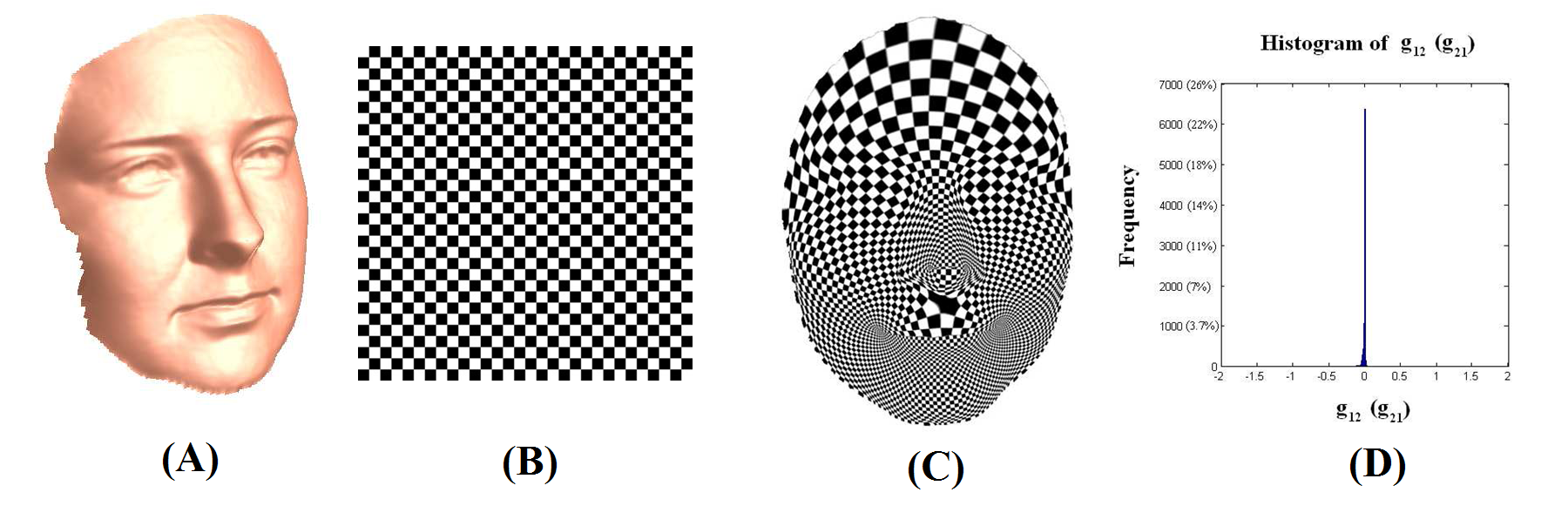
Intuitively, a map is conformal if it preserves the inner product of the tangent vectors up to a scaling factor, called the conformal factor, . An immediate consequence is that every conformal map preserves angles. Figure 1 gives an example of conformal parameterization of a human face. (A) shows a human face. It is conformally parameterized onto the 2D rectangle as shown in (B). We map the texture in (B) onto the surface, as shown in (C). Note that the right angle structure of the checkerboard texture is well-preserved. (D) shows the histogram of (or ) of the Riemannian metric. It is concentrated at 0, meaning that the mapping is conformal.
3.2. Curvatures of a Riemann surface
We next briefly describe the concept of curvatures on a Riemann surface. Given a Riemann surface , the normal curvature in some direction is the reciprocal of the radius of the circle that best approximate a normal slice of the surface in that direction. For smooth surface, it can be computed from a symmetric matrix , called the Weingarten matrix, by:
| (6) |
for any unit length vector in the tangent plane of the surface.
The principal curvatures, principal directions, mean curvatures and Gaussian curvatures can be defined by the eigenvalues and eigenvectors of . Let be the eigenvalues of and , be the eigenvectors of . Then, and are called the principal curvatures; and are called the principal directions. The mean curvature is defined as the average of the principal curvatures:
| (7) |
The Gaussian curvature is defined as the product of the principal curvatures:
| (8) |
With the conformal parameterization of , the Gaussian curvature and the mean curvature can be computed easily:
| (9) |
where is the conformal factor. And
| (10) |
where and is the (unit) surface normal.
It turns out the mean curvature together with the conformal factor are two geometric quantities fully describing the surface .
4. Surface representation by conformal factor and mean curvature
In this section, we will describe how a Riemann surface can be represented by its conformal factor and mean curvature .
Every Riemann surface is locally Euclidean, and hence it can be locally parametrized. Under the parameterization, a Riemann surface embedded in can be represented by the position vector :
| (11) |
According to the Riemann surface theory, the surface can be determined uniquely (up to a rigid motion) by its first fundamental form and second fundamental form. The first fundamental form can be written as follows:
| (12) |
where , and .
If is a conformal parameterization, and , where is the conformal factor. Hence,
| (13) |
The second fundamental form can be written as follows:
| (14) |
where , and ( is the unit surface normal).
Now, our goal is to find geometric quantities which can determine the position vector .
Let (), , , and .
Suppose is a conformal parameterization, then we must have the following:
| (15) |
Besides, the natural frame must satisfy certain equations. Consider . Then, the natural frame satisfies:
| (16) |
Clearly, the natural frame can be determined by the conformal factor , mean curvature and . Besides, can as well be determined by and through the Codazzi equation:
| (17) |
Differentiate equation (17) with respect to , we obtain
| (18) |
Given the value of on the boundary neighborhood , the natural frame can be found by solving the system of partial differential equation (16). The position vector can be reconstructed by integrating the natural frame. Therefore, the mean curvature and conformal factor are two geometric quantities fully determining a Riemann surface. Given a Riemann surface , its associated () can be computed. Conversely, given (), the associated Riemann surface can be reconstructed. We call the pair () the - representation of .
The above discussion can be summarized by the following theorem.
Theorem 4.1 (- representation).
Let be an open Riemann surface with mean curvature . Let be the conformal parameterization of with conformal factor . Suppose is a (small) boundary neighborhood of . Given the boundary value of , is uniquely determined by and .
5. Surface inpainting
In this section, we will describe a surface inpainting algorithm based on the - representation of the surface .
Suppose is an incomplete 3D surface model with holes. Let be the occluded region. Our goal is to obtain a restored surface with holes filled based on the surface geometry, so that the basic geometry of the surface can be smoothly patched. Following conventional image inpainting algorithms, we first take an initial surface with the holes roughly filled. Computationally, it can be done by creating a patch piecewise linearly with boundary vertices given by . is then iteratively modified to obtain a satisfactory inpainted surface .
One way to modify is to update the position vector of iteratively. However, this method does not consider the essential geometric information of the surface. We therefore propose to inpaint the surface by considering the conformal factor and mean curvature , which are the two essential geometric quantities determining a Riemann surface.
Let be the conformal parameterization of . We can compute the conformal factor of which is given by:
| (19) |
Suppose be the mean curvature of . Then, (, ) determines . As expected, the scalar functions and are not smooth on the occluded region in the conformal parameter domain. Our goal is to smooth out (or inpaint) and on the occluded region , while preserving the value of them on the non-occluded region .
The conformal factor and mean curvature are smooth scalar functions defined on the 2D conformal parameter domain. To ensure the smoothness of the inpainted mean curvature and conformal factor , the following inpainting model is applied:
| (20) |
subject to the constraint that:
| (21) |
Also, we apply the same inpainting model for :
| (22) |
subject to the constraint that:
| (23) |
By minimizing the variational models (20) and (22), we obtain an optimal (inpainted) conformal factor and . The surface associated with the pair can then be reconstructed, as described in the last subsection, to obtain an inpainted surface . The surface holes will be effectively filled, with the basic geometry of the surface smoothly patched.
| (24) |
subject to and .
6. Numerical algorithms
In this section, we will describe how the proposed algorithms can be implemented. We will firstly describe how the - representation can be implemented. We will then explain how the surface inpainting algorithm can be implemented.
6.1. Numerical implementation of - representation
Given a surface mesh , the - representation of can be computed easily using the conformal parameterization of . Many conformal parameterization algorithms have recently been developed and some of them are available online. We will not explain the conformal parameterizations in this paper, but refer the readers to [28, 29, 30, 32, 33, 34] for details. In this work, we use the algorithm proposed in [34] to obtain the conformal parameterization of onto the rectangular conformal parameter domain .
Let be the conformal parameterization of the surface mesh . We consider the finite difference discretization of the partial derivatives on the rectangular conformal parameter domain . Let , and . We denote and . Using equation (12), the conformal factor can be computed by:
| (25) |
And using equation (10), the mean curvature can be computed by:
| (26) |
where:
| (27) |
Conversely, given the - representation of , we can reconstruct the surface by solving the equation (16). Let be the natural frame at . Consider the central difference discretization of and as follows:
| (28) |
Hence, can be computed for all . Together with the boundary conditions, the natural frame can then be computed by solving the following linear system, which approximates the solution of the equation (16):
| (29) |
Once the natural frame is obtained, the position vector (and hence the surface mesh ) can be reconstructed by solving the linear system (with the given boundary conditions):
| (30) |
6.2. Numerical implementation of surface inpainting
Given a surface mesh with holes , we first obtain an initial mesh with the holes roughly filled. It can be obtained by the delaunay triangulation of the boundary vertices of the surface holes. The - representation of can then be computed, which are two non-smooth scalar functions of the conformal factor and mean curvature . We then inpaint (or smooth out) and at the occluded regions on the conformal parameter domain, using the inpainting models (20) and (22).
Consider the discretization of the Laplacian on the conformal parameter domain as follows:
With this discretization, the inpainting models on and can be implemented as follows:
| (31) |
with the constraints that and for all that are not in the occluded regions. is the time step.
7. Experimental results
To examine the effectiveness of the proposed method, we have tested our algorithms on synthetic data together with real surface data. In this section, we will describe the experimental results in details.
7.1. Surface reconstruction from - representation
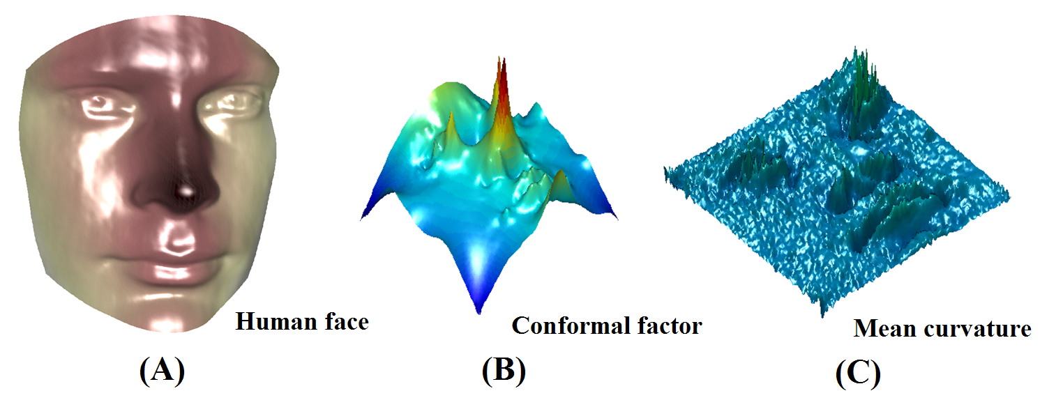
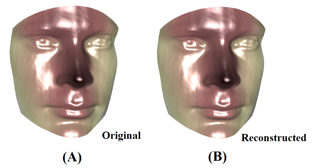
We first examine how well the - representation can represent a Riemann surface. In Figure 2, we compute the conformal factor and mean curvature of a human face. This gives the - representation of the human face. Using - representation, we can accurately reconstruct the original surface. The reconstructed surface is shown in Figure 5(B), which closely resembles to the original surface as shown in Figure 5(A).
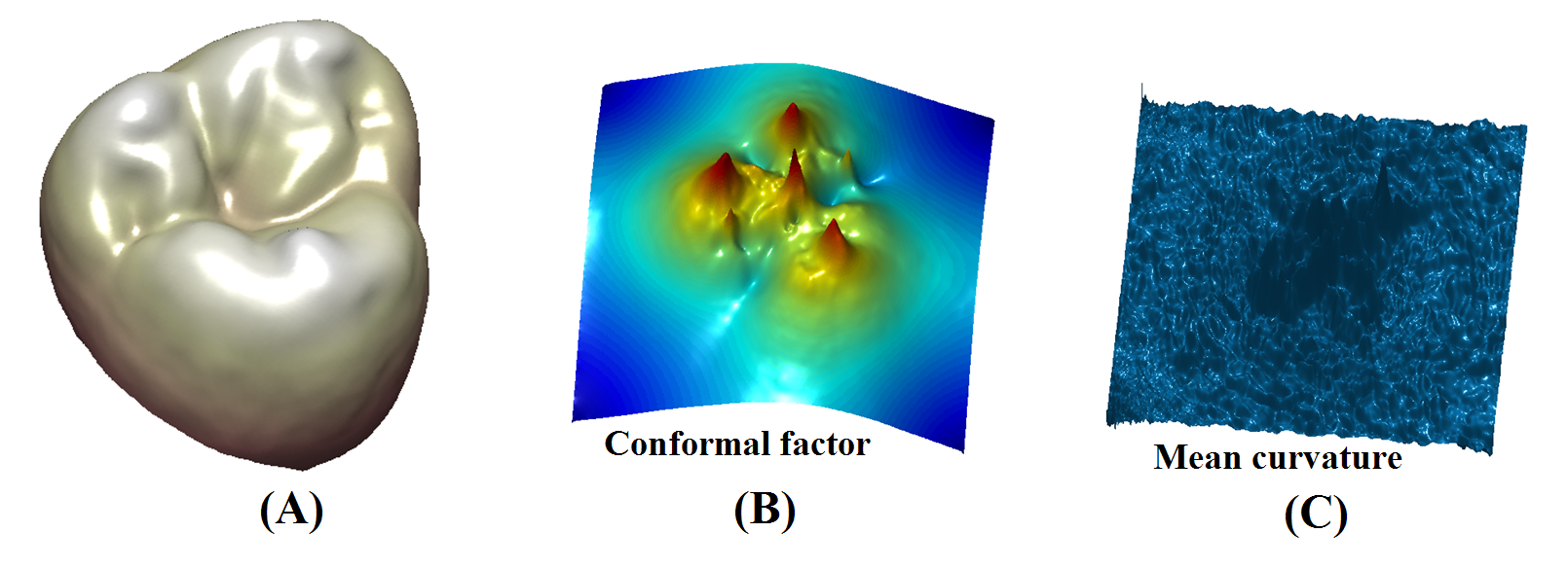
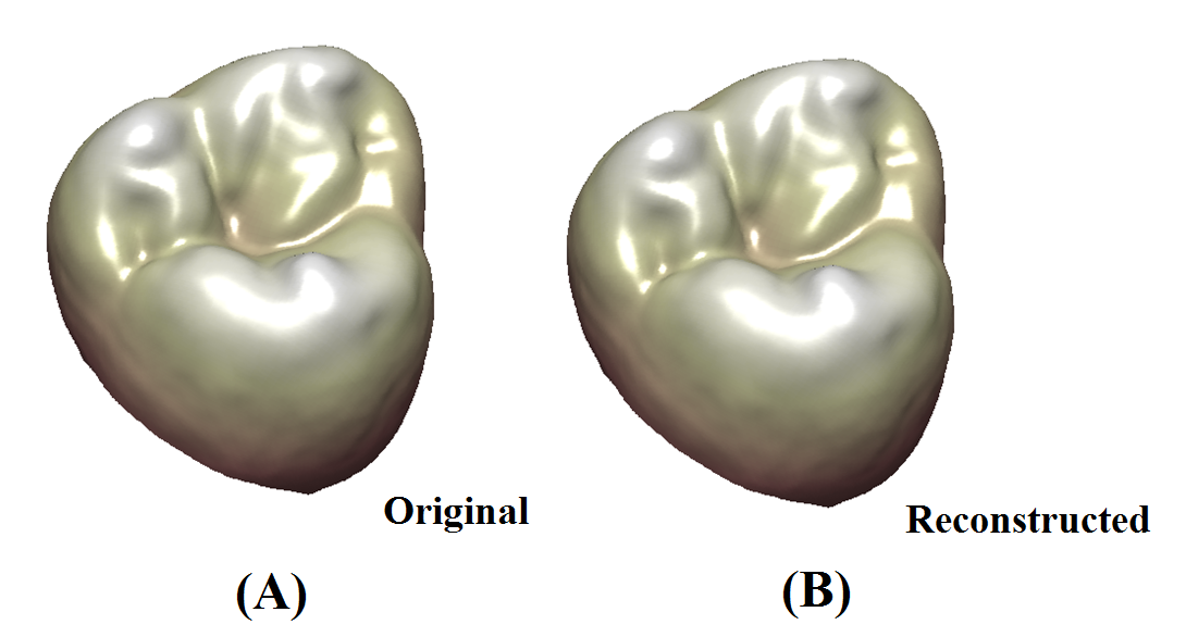
We also compute the - representation of a human tooth, as shown in Figure 3. From the - representation, the tooth surface can be effectively and accurately reconstructed. Figure 6(B), shows the reconstructed tooth surface from its - representation, which again closely resembles to the original tooth surface as shown in Figure 6(A).
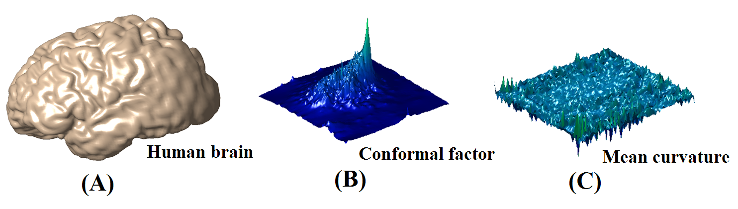
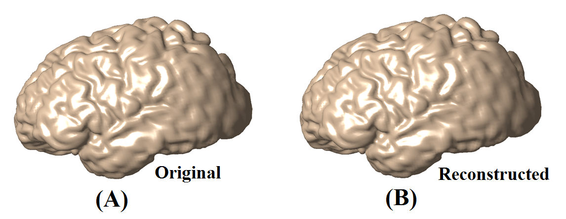
Finally, we compute the - representation of a human brain, whose geometry is complicated. The conformal factor and mean curvature of the brain surface is shown in Figure 4. From the - representation, the brain surface can be reconstructed as shown in Figure 7. The reconstructed surface is close to the original one. It demonstrates that the proposed geometric representation is effective, even for surfaces with complicated geometry.
7.2. Surface inpainting
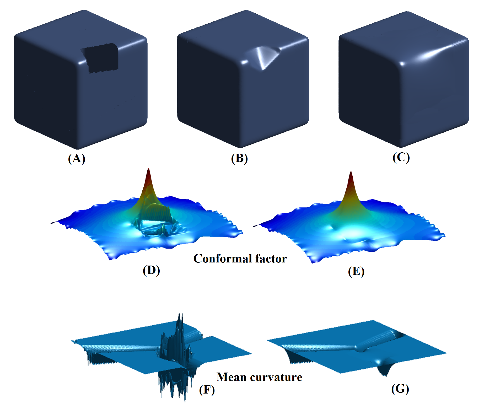
Next, we test the surface inpainting algorithm on synthetic data and real surface data. In Figure 8, we test the algorithm on a cubic surface with a hole. To inpaint the surface, a conventional way is to smoothly fill in the surface hole with its boundary representation in 3D [23, 22]. Although the surface can be smoothly filled, the inpainted surface cannot follow the surface geometry. As shown in (B), the inpainted surface generated by the conventional smooth hole-filling algorithm cannot preserve the sharp edge of the cubic surface. The sharp edge is cropped off. (C) shows the inpainted surface using our proposed conformal approach. The inpainted surface can better preserve the sharp edge. (D) and (E) shows the initial conformal factor and inpainted (smoothed) conformal factor respectively. (F) and (G) shows the initial mean curvature and inpainted (smoothed) mean curvature respectively. By inpainting the mean curvature and conformal factor, the inpainted surface follows the surface geometric pattern of the non-occluded regions of the surface.
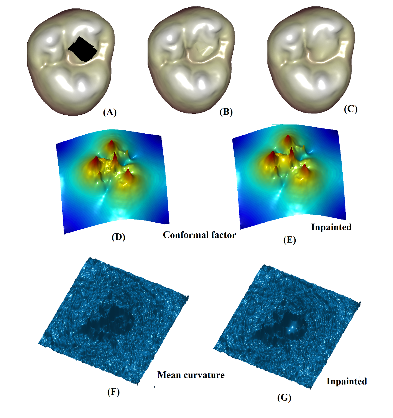
In Figure 9, we examine the proposed inpainting algorithm on a human tooth surface. (A) shows a tooth surface with an occlusion. (B) shows the inpainted surface obtained from the conventional smooth hole-filling algorithm. Again, the inpainted surface does not follow the surface geometry of the non-occluded regions of the surface. (C) shows the inpainted surface generated by our proposed inpainting method. The inpainted surface is more natural which follows the surface geometry. The basic geometry can be smoothly patched. (D) and (E) shows the initial conformal factor and inpainted (smoothed) conformal factor respectively. (F) and (G) shows the initial mean curvature and inpainted (smoothed) mean curvature respectively.
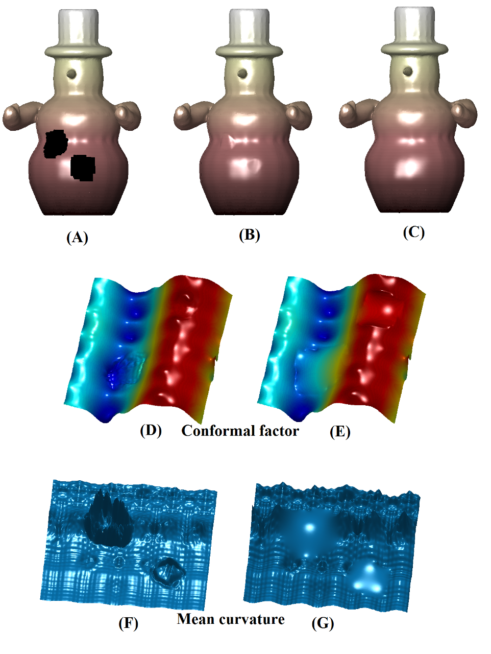
In Figure 10, we show the surface inpainting result of a snowman surface. (A) shows the snowman surface with 2 holes. (B) shows the inpainted surface obtained from the conventional smooth hole-filling algorithm. The inpainted surface patches are flatten and the inpaint surface does not follow the surface geometry. (C) shows the inpainted surface using our method. The inpainted surface is more natural which follows the surface geometry.
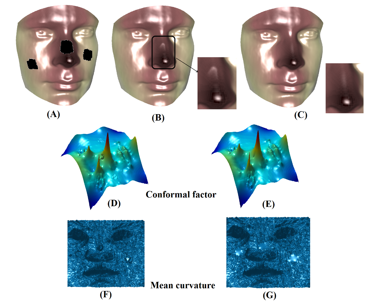
Figure 11 shows the example of surface inpainting of a human face. (A) shows a human face with 3 holes, one on the nose and two on the cheeks. (B) shows the inpainted surface obtained from the conventional smooth hole-filling algorithm. The inpainted surface is not natural and does not following the surface geometry. For example, the inpainted surface patch (inside the box) for the hole on the nose is flatten. (C) shows the inpainting result obtained by our algorithm. The reconstruct surface is more natural and follows the surface geometric pattern.
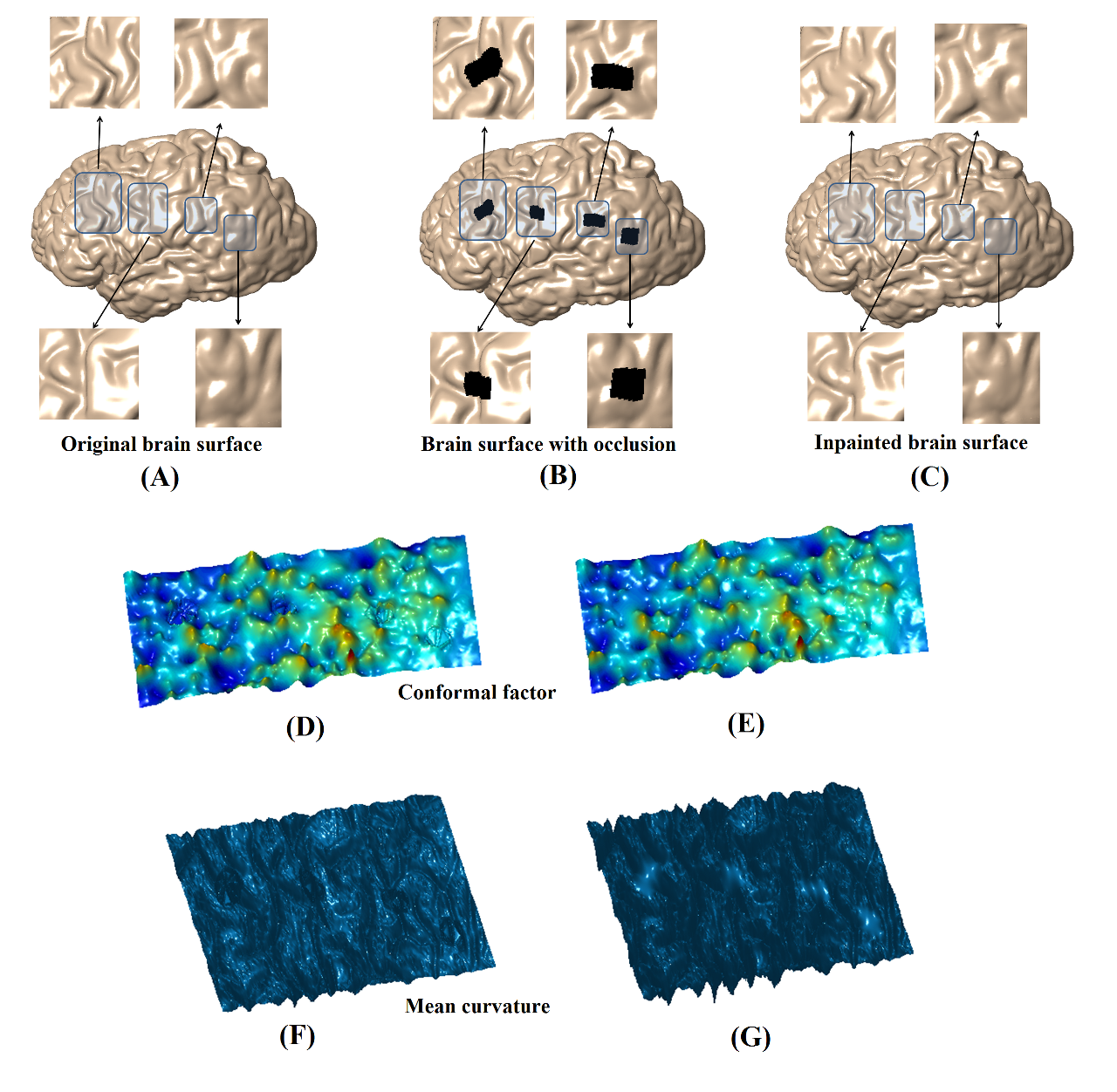
Finally, in Figure 12, we test the inpainting algorithm on a brain surface, which has more complicated geometry. (A) shows the original brain surface. We remove four regions on the brain surface, as shown in (B). The inpainted surface generated by our algorithm is shown in (C). Note that the inpainted surface patches closely resemble to the original ones (compare with (A)). This example demonstrates that our proposed inpainting algorithm perform well even on surfaces with complicated geometry.
8. Conclusion and future works
In this work, we propose a novel conformal approach for surface inpainting to fill in missing holes on an incomplete 3D surface model. It has important applications in different fields, such as in medical imaging, computer graphics and computer visions. In order to fully manipulate the surface geometry of the captured 3D model, we consider in this work a new representation of 3D surfaces based on their conformal factor and mean curvature . According to Riemann surface theory, a Riemann surface can be uniquely determined by its conformal factor and mean curvature up to a rigid motion. Given a Riemann surface , its mean curvature and conformal factor can be computed easily through its conformal parameterization. Conversely, given and , a Riemann surface can be uniquely reconstructed by solving the Gauss-Codazzi equation on the conformal parameter domain. Hence, the conformal factor and the mean curvature are two geometric quantities fully describing the surface. In this paper, we develop a numerical algorithm to reconstruct surfaces from their conformal factor and mean curvature by solving systems of linear equations. Given the - representation of an incomplete surface, the problem of surface inpainting can be reformulated into the image inpainting problem of and on the conformal parameter domain. Using the conventional image inpainting techniques, both and can be inpainted on the parameter domain. A Riemann surface can then be reconstructed which restores the 3D surface with surface holes. Since the inpainting model is based on the geometric quantities and , the restored surface follows the surface geometric pattern as much as possible. We test the proposed algorithm on synthetic data, 3D human face data and MRI-derived brain surfaces. Experimental results show that our algorithm can effectively inpaint surface holes based on the geometry of the surface to restore the incomplete 3D surface models.
Besides, we observe from our experiments that the - representation of a surface is a useful geometric representation of a surface mesh capturing the most essential geometric information. By manipulating and , the surface mesh can be edited based on the surface geometry. Thus, we believe there are several potential applications of this representation to other surface mesh editing problems, such as surface mesh compression, surface mesh denoising and so on. In the future, we will consider applying the - representation for surface stitching. We will also consider extending the - representation to point cloud. With that, point cloud compression, point cloud inpainting and point cloud denoising can be easily achieved.
References
- [1] T. F. Chan and J. Shen: Variational restoration of non-flat image features: models and algorithms. SIAM Journal on Applied Mathematics, 61(4):1338-1361, 2001.
- [2] T. F. Chan and J. Shen: Mathematical models for local non-texture inpaintings. SIAM Journal on Applied Mathematics, 62(3):1019-1043, 2001.
- [3] S. Esedoglu and J.-H. Shen: Digital inpainting based on the Mumford-Shah-Euler image model. Eureopean Journal on Applied Mathematics, 13:4, pp. 353-370, 2002.
- [4] T.F. Chan and J. Shen: Variational Image Inpainting. Communications in Pure and Applied Mathematics, 58, 579-619, 2005.
- [5] T.F. Chan, S.H. Kang, and J. Shen: Euler s elastica and curvature-based inpainting. SIAM Journal on Applied Mathematics, Vol. 63, Nr.2, pp.564 592, 2002.
- [6] S. Masnou and J. Morel: Level Lines based Disocclusion. 5th IEEE International Conference on Image Processing, Chicago, IL, Oct. 4-7, 1998, pp.259 263, 1998.
- [7] M. Bertalmio, A.L. Bertozzi, and G. Sapiro: Navier-Stokes, fluid dynamics, and image and video inpainting. Proceedings of the 2001 IEEE Computer Society Conference on Computer Vision and Pattern Recognition, 1, 355-362, 2001.
- [8] T.F. Chan, J.-H. Shen, and H.-M. Zhou: Total variation wavelet inpainting. Journal of Mathematical Imaging and Visions, 25:1, 107-125, 2006.
- [9] J. A. Dobrosotskaya, and A. L. Bertozzi: A Wavelet-Laplace Variational Technique for Image Deconvolution and Inpainting. IEEE Transaction on Image Processing, 17:5, 657 - 663, 2008
- [10] A. Tsai, Jr. A. Yezzi and A. S. Willsky: Curve evolution implementation of the Mumford-Shah functional for image segmentation, denoising, interpolation and magnification. IEEE Transaction on Image Processing, 10(8):11691186, 2001.
- [11] M. Desbrun, M. Meyer, P. Schr der, A.H. Barr: Implicit fairing of irregular meshes using diffusion and curvature flow. Proceeding of SIGGRAPH, 317-324, 1999
- [12] G. Taubin: Geometric signal processing on polygonal meshes. Eurographics , 2000
- [13] P. Smereka: Semi implicit level set methods curvature surface diffusion motion. Journal of Scientific Computing, 19, 439 456, 2003.
- [14] M. Desbrun, M. Meyer, P. Schr der, A.H. Barr: Anisotropic feature preserving denoising of height fields and bivariate data. Graphics Interface, 2000.
- [15] M. Desbrun, M. Meyer, P. Schr der, A.H. Barr: Discrete differential geometry operators in nD. Proceedings on Vis. Math 02 Berlin Germany, (2002).
- [16] U. Clarenz, U. Diewald amd M. Rumpf: Anisotropic diffusion in surface processing. Proceedings of IEEE Visualization 2000, 397 405, 2000.
- [17] C. L. Bajaj and G. Xu: Anisotropic diffusion of subdivision surfaces and functions on surfaces. ACM Transaction on Graphics, 22, 4 32, 2003.
- [18] T. Tasdizen, R. Whitaker, P. Burchard and S. Osher: Geometric surface processing via anisotropic diffusion of normals. IEEE Visualization, 125 132, 2002.
- [19] T. Tasdizen, R. Whitaker, P. Burchard and S. Osher: Geometric surface processing via normal maps. ACM Transactions on Graphics, 22,1012 1033, 2003.
- [20] V. Caselles, G. Haro, G. Sapiro, J. Verdera: On geometric variational models for inpainting surface holes. Journal of Computer Vision and Image Understanding archive, 111:3, 351-373, 2008
- [21] J. Verdera , V. Caselles , M. Bertalmio , G. Sapiro: Inpainting Surface Holes. International Conference on Image Processing, 903–906, 2003
- [22] J. Davis, S. Marschner, M. Garr, and M. Levoy: Filling holes in complex surfaces using volumetric diffusion. First International Symposium on 3D Data Processing, Visualization, and Transmission, June 2002.
- [23] U. Clarenz, U. Diewald, G. Dziuk, M. Rumpf and R. Rusu: A finite element method for surface restoration with smooth boundary conditions.. Computer Aided Geometric Design 21, 5 (2004), 427 445.
- [24] A. Sharf, M. Alexa, D. Cohen: Context-based surface completion.. ACM Transaction on Graphics, 23, 3 (2004), 878 887.
- [25] V. Savchenko and N. Kojekine: An approach to blend surfaces.. Advances in Modeling, Animation and Rendering (2002), 139 150.
- [26] M. K. Hurdal and K. Stephenson: Discrete conformal methods for cortical brain flattening, Neuroimage, 45:86–98, 2009.
- [27] B. Fischl, M. Sereno, R. Tootell, and A. Dale: High-resolution intersubject averaging and a coordinate system for the cortical surface. Human Brain Mapping, 8:272–284, 1999.
- [28] X. Gu, Y. Wang, T. F. Chan, P. M. Thompson, and S.-T. Yau: Genus zero surface conformal mapping and its application to brain, surface mapping. IEEE Transactions on Medical Imaging, 23(8):949–958, 2004.
- [29] Y. Wang, L. M. Lui, X. Gu, K. M. Hayashi, T. F. Chan, A. W. Toga, P. M. Thompson, and S.-T. Yau: Brain surface conformal parameterization using riemann surface structure. IEEE Transactions on Medical Imaging, 26(6):853–865, 2007.
- [30] X. Gu and S. Yau: Computing conformal structures of surfaces, Communication in Information System, 2(2):121–146, 2002.
- [31] X.F. Gu , Y. Wang , S.T. Yau: Geometric compression using Riemann surface structure, Communication in Information System, 3(3):171-182, 2004.
- [32] L.M. Lui, T.W. Wong, W. Zeng, X.F. Gu, P.M. Thompson, T.F. Chan and S.T. Yau: Optimization of Surface Registrations Using Beltrami Holomorphic Flow, Journal of Scientific Computing, 50(3), 557-585, 2012
- [33] L.M. Lui, T.W. Wong, X.F. Gu, P.M. Thompson, T.F. Chan and S.T. Yau: Hippocampal Shape Registration using Beltrami Holomorphic flow, Medical Image Computing and Computer Assisted Intervention(MICCAI), Part II, LNCS 6362, 323-330 (2010)
- [34] L.M. Lui, K.C. Lam, T.W. Wong, X.F. Gu: Beltrami Representation and its applications to texture map and video compression. arXiv:1210.8025 (http://arxiv.org/abs/1210.8025)
- [35] S. Haker, S. Angenent, A. Tannenbaum, R. Kikinis, G. Sapiro, and M. Halle: Conformal surface parameterization for texture mapping, IEEE Transaction of Visualization and Computer Graphics, 6, 181-189, 2000.