Knotted domain strings

Abstract

We construct meta-stable knotted domain strings on the surface of a soliton of the shape of a torus in 3+1 dimensions. We consider the simplest case of $\mathbb{Z}_{2}$ Wess-Zumino-type domain walls for which we can cover the torus with a domain string accompanied with an anti-domain string. In this theory, all $(p,q)$-torus knots can be realized as a linked pair of a(n) (un)knotted domain string and an anti-domain string.

1 Knotted vortex strings

More than 140 years ago, Lord Kelvin proposed an interesting idea that atoms could be conceived as stable knotted vortex loops. Although this idea was not successful as a theory of atoms, it led to the celebrated mathematical knot theory today. Knots are one of the most fascinating structures frequently appearing in Nature and they are found to be important in diverse areas of physics such as high energy physics, cosmology and condensed matter physics.

It was a long-standing question whether a stable knotted structure actually exists in a dynamical system. Indeed, until quite recently, no stable knot structures were found. In 1996, Gladikowski and Hellmund [1] as well as Faddeev and Niemi [2] found stable knot-like structures made of (stable) topological solitons, Hopfions, which are (un)knotted closed loops of vortex tubes in the Faddeev-Skyrme model [3]. The Faddeev-Skyrme model is an $O(3)$ nonlinear sigma model with the addition of a (four-derivative) Skyrme term. With the aid of the recent drastically improved computer power, they succeeded in constructing numerical solutions of Hopfions with small charges. Faddeev and Niemi [2] conjectured that all torus knots can be constructed from stable knotted vortex tubes. Soon after, Battye and Sutcliffe found beautiful higher-charged Hopfions numerically, which have both link and knot structures [4].

After the discovery in terms of numerical solutions, the knotted solitons have been studied extensively in the literature. However, all knotted solitons, known so far, are obtained from closed vortex flux tubes. The purpose of this Letter is to demonstrate the existence of a different type of knotted soliton, which lives on the surface of toroidal structures in 3+1 dimensions. Viz. we construct non-planar domain strings on the surface of a ring-shaped soliton, like a vorton [5], a superconducting string loop (spring) [6] or a $Q$-ring [7] etc.

2 The model

In [8, 9] it was proposed that non-planar domain wall networks might exist on the surface of a host soliton star which is a spherically compactified domain wall. This idea was investigated numerically in [10] in a simple concrete model having two complex scalar fields and $U(1)\times\mathbb{Z}_{n}$ global symmetry. In [10], the host soliton (star) is a large $Q$-ball [11] and an attempt was made to tile the surface of the $Q$-ball with almost-BPS planar domain-string networks in the Wess-Zumino model [12]. However, in [10] it was proven that only a few spherical polyhedra can be constructed on the surface of a sphere.

Although an attempt of tiling the domain-string network on a sphere did not turn out very successful, we can still ask whether it is possible to tile other Riemann surfaces with domain strings. Namely, how does the answer depend on the topology of the host soliton. Because we are interested in a solitonic object which may be dynamically produced, we choose a torus, $T^{2}$, which is one of the simplest geometries. Indeed, many ring-shaped solitons are known, e.g. a closed loop of the superconducting cosmic strings [5], springs [6] and Hopfions [1].

We will work in the framework of the simple model proposed in [10] which was used to construct the domain-string networks on $Q$-balls. That is, we will use a single complex scalar field $\phi$ with an effective potential of the Wess-Zumino type coupled to some other field which belongs to a host configuration. Hence, the Lagrangian contains two parts

$${\cal L}={\cal L}_{1}[A_{\mu},\psi_{i}]+{\cal L}_{2}[\psi_{i},\phi],$$ (1)

where $\mathcal{L}_{1}$ may include multiple scalar fields $\psi_{i}$ and gauge fields $A_{\mu}$ which are needed to form a stable ring soliton. The Wess-Zumino field $\phi$ couples to $\psi_{i}$ only via $\mathcal{L}_{2}$. We need not specify a particular model for $\mathcal{L}_{1}$, but we require it to have a solitonic field configuration admitting a ring-shaped profile function. The only condition which we require for one of the $\psi_{i}$’s, say $\psi_{1}$, is that it is non-zero inside and zero outside of the ring, see Fig. 1. Indeed, this is a universal property of the condensate field for the well-known vortons and springs.

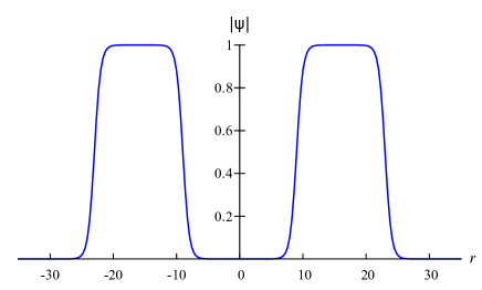
Figure 1: The cross-section profile of $\psi$ for a ring-shaped soliton at $z=0$. The ring is axially symmetric with respect to the $z$-axis.

Then, for ${\cal L}_{2}[\psi_{i},\phi]$, we consider the specific model

$${\cal L}_{2} = \frac{1}{2}|\partial_{\mu}\phi|^{2}-\beta^{2}\left|\eta[\psi_{1}]-\frac{\phi^{2}}{v^{2}}\right|^{2},$$ (2)

$$\eta[\psi_{1}] \equiv 4|\psi_{1}|^{2}\left(1-|\psi_{1}|^{2}\right).$$ (3)

As done in [10], we treat $\beta$ as a small parameter, such that the profile of the torus configuration of ${\cal L}_{1}$ receives only a negligible correction. This can be seen as follows. To be concrete, let us consider one of the simplest models as ${\cal L}_{1}$ consisting of the complex fields $(\psi_{1},\psi_{2})=(\psi,\sigma)$:

$${\cal L}_{1}[\psi,\sigma] = |\partial_{\mu}\psi|^{2}+|\partial_{\mu}\sigma|^{2}-\gamma|\psi|^{2}|\sigma|^{2}\ ,$$ (4)

$$\eta[\psi] = 4|\psi|^{2}|\sigma|^{2}=4|\psi|^{2}(1-|\psi|^{2})\ ,$$ (5)

with the constraint $|\sigma|^{2}+|\psi|^{2}=1$ and $\gamma$ takes on a positive value. The stable vorton solution in this model ($\beta=0$) was obtained in [13]. The field $\sigma=f(r)e^{ik\theta}$ is called the vorton field, and the condensate $\psi$ whose phase increases along the vorton as $\psi=g(r)e^{i(\omega t+pz)}$, with $r,\theta$ being polar coordinates. Since we just want to estimate how much the host soliton is modified by turning on a non-zero coupling, $\beta$, we simplify the problem here and consider a so-called twisted-vortex string [13] on a periodic interval, $z=2\pi/p$, instead of the vorton. Let us consider the twisted-vortex string in ${\cal L}={\cal L}_{1}+{\cal L}_{2}$. Firstly, the vacuum structure of ${\cal L}$ is not changed with respect to that of ${\cal L}_{1}$ in Eq. (5). Furthermore, all the conserved charges are independent of $\beta$. The existence of the same kinds of (host) solitonic configurations in $\mathcal{L}$ with $\beta\neq 0$ as in ${\cal L}$ with $\beta=0$ follows straightforwardly. Indeed, we obtained numerically a twisted vortex string solution which is shown Fig. 2.

Figure 2: The twisted vortex profile functions $|\psi(r)|^{2}$ (in gold/decreasing with $r$), $|\sigma(r)|^{2}$ (in violet/increasing with $r$) and $|\phi/v|^{2}$ (in blue) for $k=2$ with $\beta=0$ (dashed curves) and $\beta=v=1$ (solid curves). The parameters are chosen as $\gamma=1$, $\omega=1$ and $p=1.1$. One can increase the toroidal radius $R_{p}$ by increasing the winding number $k$ in $\mathcal{L}_{1}$.

In Fig. 2, we have chosen a relatively large value for the coupling, i.e. $\beta=1$, but the deformation of the profile functions, $\psi$ and $\sigma$, remains small. Thus we conclude that the shape of the host ring is quite insensitive to the $\beta$ coupling – even for order one values – and thus we can safely ignore the back reaction as long as $\beta$ is kept sufficiently small. There is, however, an important difference between $\beta=0$ and $\beta\neq 0$: $\phi\neq 0$ for the latter. Since $\eta[\psi_{i}]=0$ both inside and outside of the ring, $\phi$ only develops a non-zero VEV $\phi\simeq v$ near the surface of the ring, in order to minimize the energy contribution from the potential term. Clearly, there exists another configuration, namely $\phi\simeq-v$ near the surface of torus. These two configurations have exactly the same energy due to the $\mathbb{Z}_{2}$ symmetry of the model. Hence, the $\mathbb{Z}_{2}$ symmetry is spontaneously broken by the ring soliton, which gives rise to domain strings on the host ring soliton.

Once we ignore the back reaction to the host soliton, ${\cal L}_{2}$ can be seen effectively as the $2+1$ dimensional Wess-Zumino model with a $\mathbb{Z}_{2}$ discrete symmetry, where the field $\phi$ has VEVs $\langle\phi\rangle\simeq\pm v$. As well known, the Wess-Zumino model in $2+1$ dimensions admits domain strings interpolating those two vacua having tension and transverse size, respectively,

$$T=\frac{2^{5/2}}{3}\beta v,\quad d=\frac{v}{\beta}.$$ (6)

Therefore, we can take $\beta$ parametrically small keeping the size of the domain string $d$ fixed. We will choose $\beta\simeq v$ such that $d$ is of order one in the following, and hence the tension of the domain string is of order $\beta^{2}$. Since, no physical parameters depend on only $\beta$, we can keep the size of the domain strings large and choose a small value of $\beta$. In this way the back reaction is parametrically negligible and need not be a concern.

In the following, we will tile the surface of the ring soliton with these two domains.

3 Numerical calculation

We solved the partial differential equations (gradient flow equations) with a finite difference method, more precisely using a Crank-Nicolson algorithm on a $160^{2}\times 80$ square lattice times a relaxation time axis with Courant number, $\Delta t/\Delta x_{i}=0.2$:

$$-\partial_{\phi}\mathcal{E}={\rm EOM}[\nabla\phi,\phi]=\partial_{t}\phi\,,$$ (7)

such that when the configuration does not change anymore, the soliton configuration is obtained. This is the relaxation method. The spatial lattice has the lengths $60^{2}\times 30$ and stepsize $\Delta x_{i}=0.375$ and we chose $\beta=v/3=0.1$ yielding $d=\sqrt{3}$. Hence, the stepsize is small enough to resolve the domain string (there is about $4.6$ lattice points on the domain string itself). Since the Crank-Nicolson algorithm is implicit

$$\frac{1}{2}\left[-\partial_{\phi}\mathcal{E}(t)-\partial_{\phi}\mathcal{E}(t+\Delta t)\right]=\frac{\phi(t+\Delta t)-\phi(t)}{\Delta t}\,,$$ (8)

$\phi(t+\Delta t)$ needs to be calculated by means of solving a matrix equation for which we use a biconjugate gradients method. Since the equation of motion is non-linear, we linearize the equation (only for $\phi$ at time $t+\Delta t$)

$$\phi=\phi_{0}+\delta\phi\,,$$ (9)

i.e. we keep the full non-linear expression for $\phi_{0}$ but truncate $\delta\phi$ to linear order. We then iterate several times until the solution of the next time slice, $\phi(t+\Delta t)$, converges. Thereafter, the routine is continued until the variation of the field in time is small enough.

The Figs. 3–5 are obtained by the above explained Crank-Nicolson algorithm. As a check we have also carried out the same calculation using Mathematica. We obtain equally good solutions with the calculation done in Mathematica, see Figs. 6–8.

With an appropriate initial configuration, one obtains the desired results as final states of the relaxation. If the configuration is unstable, it collapses to a single vacuum. Since we obtained non-trivial domain strings by means of the relaxation, they represent stationary points of the energy.

4 Knotted domain strings

As we will explain, domain strings on the ring surface are nothing but torus knots. Therefore, they are naturally characterized by a pair of co-prime integers $(p,q)$. The number $p$ denotes the poloidal winding number (around the meridian circle), while $q$ is the toroidal winding number (around the longitudinal circle) of the torus. As well known, torus knots are prime and chiral. Torus knots with $pq>0$ are right-handed and $pq<0$ are left-handed. A $(p,q)$-knot is identical to the $(-p,-q)$-knot.

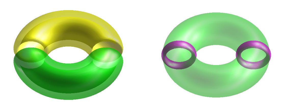
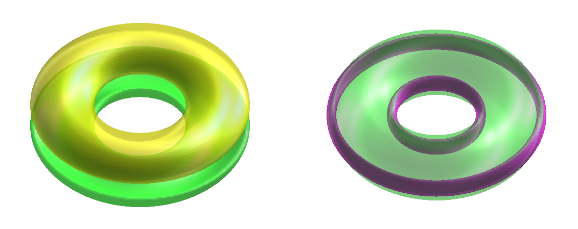
Figure 3: The left panel shows the two domains. The two domain strings (i.e. energy density isosurface) are shown in the right panel. The upper figures are for the $(1,0)$ type, i.e. poloidal strings, while the lower figures are for the $(0,1)$ type, i.e. toroidal strings.

The simplest configurations are the $(1,0)$ and $(0,1)$. These have unknotted closed domain strings sitting on the antipodal points of the torus, see Fig. 3. Clearly, the configuration $(0,1)$ is unstable against small perturbations because the smaller string loop is preferred energetically. Thus, the larger string will shrink and annihilate the smaller one since the net $\mathbb{Z}_{2}$ charge of the configuration is trivial.

The Hopf link appears for the $(1,1)$ type. The configuration is unknotted but two domain strings are singly linked which is a so-called Hopf link, see Fig. 4.

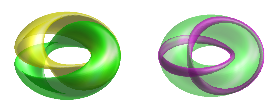
Figure 4: Hopf link $(1,1)$: The left figure shows the tiling of the surface of a torus with two domains and the right figure shows that the domain strings are linked once.

Each string loop winds both cycles of the torus once. The domain string and anti-domain string sit near the antipodal point with respect to the other on the torus. They are, however, nearly maximally separated from each other in most of the configuration.

The unknotted but doubly linked strings are obtained for the $(2,1)$ and $(1,2)$ cases. They are called Solomon’s links, see Fig. 5.

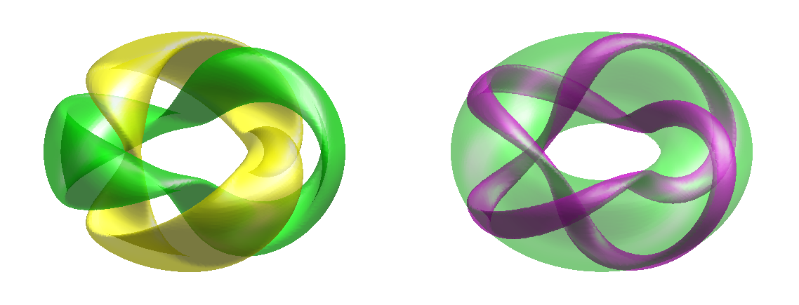
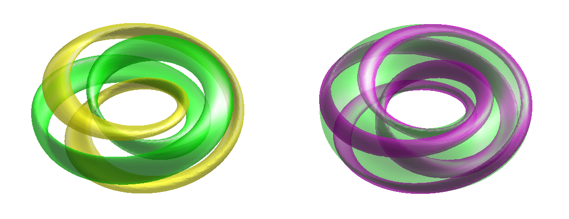
Figure 5: Solomon’s links: The upper figures show the $(2,1)$ configuration and the lower ones show the $(1,2)$-type strings. These are unknotted but doubly linked configurations.

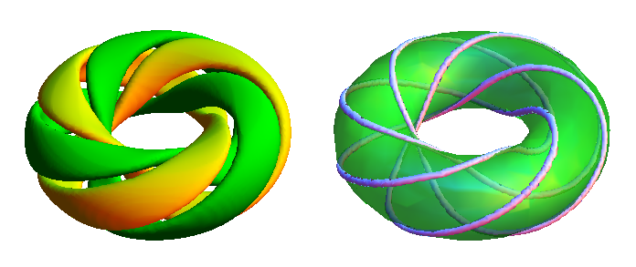
Figure 6: The sixthly linked trefoil knot with winding numbers $(3,2)$. The top-left figure shows the region where ${\rm Re}[\phi]>0$ which is a trefoil form. The top-right figure displays the two linked trefoil domain strings in the view from above. The bottom-left figure shows the two domains on the torus surface and the bottom-right figure is a 3D view of the trefoil knots.

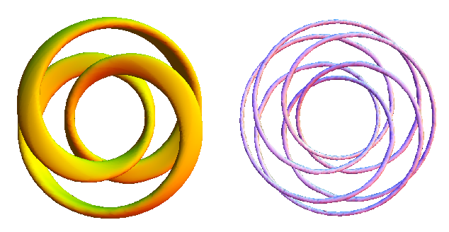
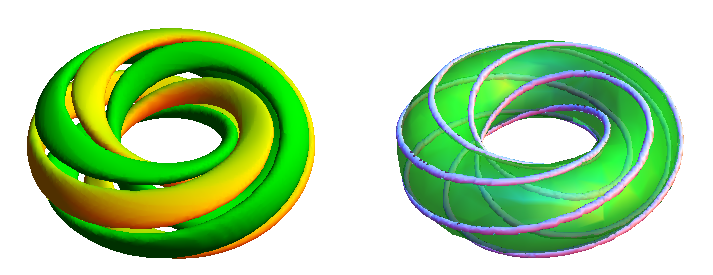
Figure 7: The sixthly linked trefoil knot with winding numbers $(2,3)$. See the caption of Fig. 6.

The next example is the linked trefoil which is the simplest knotted structure among the torus knots. Namely, they are characterized by winding numbers $(3,2)$ and $(2,3)$, see Figs. 6 and 7. The linking number is the product of $p$ and $q$. Hence, both these trefoils are linked 6 times. In [2], it was conjectured that all torus knots can be constructed as Hopfions in the Faddeev-Skyrme model, but to the best of our knowledge our solutions are the first ones realizing both the $(3,2)$ and the $(2,3)$ configuration. For these torus knots and the remaining higher-winding ones, we have decreased the domain string width $d\simeq 1$, instead of $\sqrt{3}$ as used in the lower-winding cases, see Eq. (10).

The last example is the linked knot with winding numbers $(4,3)$ and linking number 12, see Fig. 8.

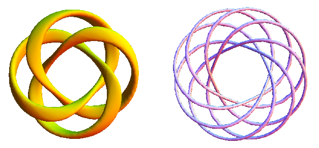
Figure 8: The linked knot with winding numbers $(4,3)$.

5 Stability

There are two types of stability issues. The first is regarding the impact of the presence of the domain strings on the host solitons; that is, the fields have a mutual coupling that potentially could destabilize the host soliton. This issue has been demonstrated in detail above to depend on $\beta^{2}$ and be parametrically unimportant for vanishing $\beta$. To this end, let us point out that the host soliton is stable for $\beta=0$. Therefore, size- or shape-changing modes of the host soliton are massive in the case of $\beta=0$. Let the shape-mode be gapped with mass $m^{2}>0$. Once $\beta>0$ is turned on, $m$ changes accordingly and could potentially become tachyonic. However, by continuity, an infinitesimal change in $\beta>0$ from $\beta=0$ is not expected to be able to drive $m^{2}$ negative from a finite positive value. Thus for sufficiently small $\beta$ this type of instability is prevented. The other type of instability is due to the domain strings coming in pairs of string and anti-string. We will discuss this issue below.

Since ${\cal L}_{2}$ is effectively the $\mathbb{Z}_{2}$ Wess-Zumino model on the surface of a torus, the domain strings are characterized by two winding numbers, $(p,q)$, and also by the $\mathbb{Z}_{2}$ charge. Each string has either $+$ or $-$ $\mathbb{Z}_{2}$ charge. All configurations are topologically protected in the sense of the topologically non-trivial winding numbers $(p,q)$. However, since the torus surface is periodic, a single domain string is always accompanied by its anti-domain string. Hence, the total $\mathbb{Z}_{2}$ charge is trivial. Therefore, all the domain-string configurations which we have obtained in this letter are non-topological solitons.

Although their stability is granted by topology, we expect meta-stability and thus a sufficiently long life time of the configurations. This is due to the interaction between the $\mathbb{Z}_{2}$ kinks being exponentially suppressed as $V\sim\exp(-mL)$ where $m$ is a mass parameter which is of the order of the inverse kink width $d$ and $L$ denotes the separation distance of the $\mathbb{Z}_{2}$ kink and anti-kink. Indeed, the asymptotic potential can be numerically calculated with the superposition of the well-known kink and anti-kink solutions, and one finds that the potential has a large plateau in the asymptotic region. Only when the two kinks are close enough together, they feel a finite (non-negligible) attractive force. Since the two domain strings in all the constructed configurations are nearly maximally separated, the attractive interactions among them are small enough to render the configurations sufficiently stable. An exception, however, is the unknot of type $(0,1)$ which clearly is unstable against small perturbations.

When we increase either winding number, $p$ or $q$, a fixed size torus leaves less and less space for the individual domain string in order not to be too close to its anti-domain string. That is, when that happens, they will simply annihilate and leave behind a single vacuum. Hence, a crude estimate of the maximum allowed winding numbers of the strings are

$$d\ll L\sim\frac{\pi R_{\rm P}R_{\rm T}}{\sqrt{q^{2}R_{\rm T}^{2}+p^{2}R_{\rm P}^{2}}},$$ (10)

where $R_{\rm P}$ is the poloidal radius and $R_{\rm T}$ is the inner toroidal radius. Here, we chose $d=v/\beta=\sqrt{3}$ (or $d\simeq 1$ in Figs. 6–8) and $R_{\rm P,T}={\cal O}(10)$.

A further point in favor of the argument of stability is the numerical method used being a relaxation method. The relaxation method only stops and gives a configuration when a locally stable, or alternatively long-lived metastable configuration has been obtained.

There are three options for improving the stability. i) Charging the domain strings in such away that they repel or attract each other by some kind of confining force. ii) A stable bound state of a string and anti-string may exist. iii) Considering a periodic model as ${\cal L}_{2}$. All of these may be realized by changing the model ${\cal L}_{2}$. The third option might be the best choice. As an example, we can choose a modified sine-Gordon model for ${\cal L}_{2}$ with a periodic field à la axion field. Because the sine-Gordon model is periodic by definition, we do not need the anti-domain string. Thus, the single domain string can exist by itself in such a model. We will report on this possibility elsewhere.

6 Conclusions

In this Letter, we obtained numerical solutions of new knotted domain strings on the surface of a ring soliton in $3+1$ dimensions. We found several torus knots with winding numbers $(1,0)$, $(2,1)$, $(3,2)$ and $(4,3)$. With these results, we expect that all torus knots, i.e. with any co-prime integers $(p,q)$ can be constructed as domain strings in dynamical systems . It is known that lots of complicated three-dimensional shapes can be formed as solitons, for instance, the Buckyball was found as a higher-charged Skyrmion. Even on such a complicated two-dimensional surface as host soliton, we may construct domain strings. We would like to emphasize that this is indeed a doable task since the method of [10] is really simple and changing the topology of the host soliton does not lead to any difficulties. We hope that the knotted domain strings found here will open new research directions in many areas of physics and mathematics.

Note added: Ref. [14] appeared recently on the arXiv and contains similar torus-knots, however in a different model.

References

- [1] J. Gladikowski and M. Hellmund, “Static solitons with nonzero Hopf number,” Phys. Rev. D 56, 5194 (1997) [hep-th/9609035].
- [2] L. D. Faddeev and A. J. Niemi, “Knots and particles,” Nature 387, 58 (1997) [hep-th/9610193].
- [3] L. Faddeev, Princeton Report No. IAS-75-QS70, 1975
- [4] R. A. Battye and P. M. Sutcliffe, “Knots as stable soliton solutions in a three-dimensional classical field theory.,” Phys. Rev. Lett. 81, 4798 (1998) [hep-th/9808129].
- [5] R. L. Davis and E. P. S. Shellard, “Cosmic Vortons,” Nucl. Phys. B 323, 209 (1989).
- [6] E. J. Copeland, N. Turok and M. Hindmarsh, “Dynamics Of Superconducting Cosmic Strings,” Phys. Rev. Lett. 58, 1910 (1987).
- [7] M. Axenides, “Semitopological Q rings,” hep-ph/0111354.
- [8] D. Bazeia and F. A. Brito, “Tiling the plane without supersymmetry,” Phys. Rev. Lett. 84, 1094 (2000) [hep-th/9908090].
- [9] F. A. Brito and D. Bazeia, “Network of domain walls on soliton stars,” Phys. Rev. D 64, 065022 (2001) [hep-th/0105296].
- [10] P. Sutcliffe, “Domain wall networks on solitons,” Phys. Rev. D 68, 085004 (2003) [hep-th/0305198].
- [11] S. R. Coleman, “Q Balls,” Nucl. Phys. B 262, 263 (1985) [Erratum-ibid. B 269, 744 (1986)].
- [12] P. M. Saffin, “Tiling with almost BPS junctions,” Phys. Rev. Lett. 83, 4249 (1999) [hep-th/9907066].
- [13] E. Radu and M. S. Volkov, “Existence of stationary, non-radiating ring solitons in field theory: knots and vortons,” Phys. Rept. 468, 101 (2008) [arXiv:0804.1357 [hep-th]].
- [14] M. Kobayashi and M. Nitta, “Torus knots as Hopfions,” arXiv:1304.6021 [hep-th].