Subhaloes gone Notts: Spin across subhaloes and finders

Abstract

We present a study of a comparison of spin distributions of subhaloes found associated with a host halo. The subhaloes are found within two cosmological simulation families of Milky Way-like galaxies, namely the Aquarius and GHALO simulations. These two simulations use different gravity codes and cosmologies. We employ ten different substructure finders, which span a wide range of methodologies from simple overdensity in configuration space to full 6-d phase space analysis of particles. We subject the results to a common post-processing pipeline to analyse the results in a consistent manner, recovering the dimensionless spin parameter. We find that spin distribution is an excellent indicator of how well the removal of background particles (unbinding) has been carried out. We also find that the spin distribution decreases for substructure the nearer they are to the host halo’s, and that the value of the spin parameter rises with enclosed mass towards the edge of the substructure. Finally subhaloes are less rotationally supported than field haloes, with the peak of the spin distribution having a lower spin parameter.

1 Introduction

Within the hierarchical galaxy formation model, dark matter haloes are thought to play the role of gravitational building blocks, within which baryonic diffuse matter collapses and becomes detectable (White & Rees, 1978; White & Frenk, 1991). Gravitational processes that determine the abundance, the internal structure and kinematics, and the formation paths of these dark haloes within the cosmological framework, can be simulated in great detail using $N$-body methods. However, the condensation of gas associated with these haloes, eventually leading to stars and galaxies we see today, is still at the frontier of present research efforts. A first exploration of the (cosmological) formation of disc galaxies has been presented in Fall & Efstathiou (1980), where it was shown that galactic spin is linked to the surrounding larger scale structure (e.g. the parent halo). In particular, the general theory put forward by Fall & Efstathiou reproduces galactic discs with roughly the right sizes, if specific angular momentum is conserved, as baryons contract to form a disc (previously suggested by Mestel (1963)) and if baryons and dark matter initially share the same distribution of specific angular momentum.

While the theory has subsequently been refined, it always included (and still includes) such a coupling between the parent halo’s angular momentum and the resulting galactic disc (cf. Dalcanton et al. (1997); Mo et al. (1998); Navarro & Steinmetz (2000); Abadi et al. (2003); Bett et al. (2010) ). The origin of the halo’s spin can now be understood in terms of tidal torque theory in which protohaloes gain angular momentum from the surrounding shear field (e.g., Peebles (1969); White (1984); Barnes & Efstathiou (1987)) as well as by the build-up of angular momentum through the cumulative transfer of angular momentum from subhalo accretion (Vitvitska et al., 2002). Whichever way the halo gains its spin, it is a crucial ingredient for galaxy formation and all semi-analytical modelling of it (Kauffmann et al., 1993, 1997; Frenk et al., 1997; Cole et al., 2000; Benson et al., 2001; Croton et al., 2006; De Lucia & Blaizot, 2007; Bower et al., 2006; Bertone et al., 2007; Font et al., 2008; Benson, 2012).

A number of studies have been performed on the spin of haloes, in particular studies by Peebles (1969); Bullock et al. (2001); Hetznecker & Burkert (2006); Bett et al. (2007); Macciò et al. (2007); Gottlöber & Yepes (2007); Knebe & Power (2008); Antonuccio-Delogu et al. (2010); Wang et al. (2011); Trowland et al. (2012); Lacerna & Padilla (2012); Bryan et al. (2012) but so far little has been done on subhaloes. These studies look at the spin of individual dark matter haloes found in cosmological simulations and generally do not focus on the substructure, or differences between substructure definition due to lack of resolution. Here we present a comparison of spin parameters across a number of detected subhaloes found by a variety of substructure finders. The finders use many different techniques to detect substructure within a larger host halo. This is a follow-up to a more general paper comparing the recovery of structure by different finders in Onions et al. (2012) and its predecessor Knebe et al. (2011).

The techniques studied here for finding substructures include real-space, phase-space, velocity-space finders, as well as finders employing a Voronoi tessellation, tracking haloes across time using snapshots, friends-of-friends techniques, and refined meshes as the starting point for locating substructure. With such a variety of mechanisms and algorithms, there is little chance of any systematic source of errors in the collection of substructure distorting the result. Subhaloes are particularly subject to distortion and evolution, more so than haloes because, by definition, they reside within a host halo with which they tidally interact. This can affect their structure and other parameters, and in this case we are particularly interested in the spin properties. We quantify the spin with the parameter $\lambda$, a dimensionless quantity that characterises the spin properties of a halo and is explained in more detail in Section 2.

The rest of the paper is structured as follows. We first describe the methods used to quantify the spin of the halo in Section 2. The data we used is described in Section 3. Next we look at the overall properties of the spin in Section 4.1. Then we look at the correlation between the host halo and the subhaloes spin in subsection 4.2. Finally we look at how the spin is built up within the subhalo as a function of mass in subsection 4.3. We conclude in Section 5.

2 Method

2.1 Spin parameter

The dimensionless spin parameter gives an indication of how much a gravitationally bound collection of particles is supported in equilibrium via net rotation compared to its internal velocity dispersion. The spin parameter varies between 0, for a structure negligibly supported by rotation, to values of order 1 where it is completely rotationally supported, and in practice maximum values are usually $\lambda\approx 0.4$ (Frenk & White, 2012). Values larger than 1 are unstable structures not in equilibrium.

There are two variants of the spin parameter that are in common use. Peebles (1969) proposed to parametrise the spin using the expression given in Equation 1.

$$\lambda=\frac{J\sqrt{\left|E\right|}}{GM^{5/2}}$$ (1)

where $J$ is total angular momentum, $E$ the energy and $M$ the mass of the structure. In isolated haloes, all of these quantities are conserved, which gives the definition a time independence.

Bett et al. (2007) measured the Peeble’s spin parameter and fitted an expression to the distribution for haloes extracted from the Millennium simulation (Springel et al., 2005); that is characterised by Equation 2

$$P(\log\lambda)=A\left(\frac{\lambda}{\lambda_{0}}\right)^{3}\exp\left[-\alpha\left(\frac{\lambda}{\lambda_{0}}\right)^{3/\alpha}\right]$$ (2)

where A is

$$A=3\ln 10\frac{\alpha^{\alpha-1}}{\Gamma(\alpha)}$$ (3)

The variables $\lambda_{0}$ and $\alpha$ are free parameters, and $\Gamma(\alpha)$ is the gamma function. The best fit they found for field haloes was with $\lambda_{0}=0.04326$ and $\alpha=2.509$.

Bullock et al. (2001) proposed a different definition of the spin parameter, $\lambda^{\prime}$, expressed in Equation 4. As it is not dependent on measuring the energy it is somewhat faster to calculate when dealing with large numbers of haloes.

$$\lambda^{\prime}=\frac{J}{\sqrt{2}MRV}$$ (4)

Here $J$ is the angular momentum within the enclosing sphere of virial radius $R$ and virial mass $M$, and $V$ is the circular velocity at the virial radius ($V^{2}=GM/R$). The Bullock spin parameter is more robust to the position of the outer radius of the structure. Bullock proposes a fitting function to the distribution as described in Equation 5 which was based on one from Barnes & Efstathiou (1987).

$$P(\lambda^{\prime})=\frac{1}{\lambda^{\prime}\sqrt{2\pi}\sigma}\exp\left(-\frac{\ln^{2}(\lambda^{\prime}/\lambda_{0}^{\prime})}{{2\sigma^{2}}}\right)$$ (5)

This has free parameters $\lambda_{0}^{\prime}$ and $\sigma$ and Bullock et al. (2001) found a best fit for field haloes at values of $\lambda_{0}^{\prime}=0.035$ and $\sigma=0.5$.

The Peebles calculation is perhaps more well defined for a given set of particles, as it is calculated directly from the particles properties, whereas the Bullock parameter is easier to calculate from gross halo statistics, and is not dependant on the density profile. For more comparisons of the two parameters the reader is referred to Hetznecker & Burkert (2006)

2.2 The SubHalo Finders

In this section we briefly list the halo finders that took part in the comparison project. More details about the specific algorithms are available in Onions et al. (2012) and the articles referenced therein.

• adaptahop (Tweed) is a configuration space over density finder (Aubert et al., 2004; Tweed et al., 2009).

• ahf (Knollmann & Knebe) is a configuration space spherical overdensity adaptive mesh finder (Gill et al., 2004; Knollmann & Knebe, 2009).

• grasshopper (GRadient ASSisted HOP) (Stadel) is a reworking of the skid group finder(Stadel, 2001) and appears within our wider comparison for the first time here, and so is described in more detail. It takes an approach like the HOP algorithm (Eisenstein & Hut, 1998) and reproduces the initial grouping of skid in two computational steps. First densities are calculated for all particles as before using the Monaghan M3 SPH kernel over 80 nearest neighbours. Second, for each particle, the gradient of the density is calculated in a way that cancels the so-called E0 error in the gradient (Read et al., 2010), by using the gradient of the M3 kernel. Then, given that the neighbours lie within a ball of radius $2h$, we create a link from this particle to the closest neighbour to the point a distance $h$ in the direction of the gradient.

  After links have been created, each particle follows the chain of links until is reaches a cycle, marking oscillation about the density peak of the group. Finally since noise below a gravitational softening length causes a lot of artificial density peaks we search for particles of a cycle which are within a distance $\tau$ of any other particles in a cycle. The parameter $\tau$ is typically set to 4 times the gravitational softening length, as was the typical case for skid. Unbinding is also performed in a nearly equivalent way to skid, but now scales as $O(n\log n)$ as opposed to $O(n^{2})$ as was the case with the original skid.

  The group finding with grasshopper is now fast enough to allow it to be performed during a simulation but gives nearly identical results to the previous skid algorithm.

• Hierarchical Bound-Tracing (hbt) (Han) is a tracking algorithm working in the time domain (Han et al., 2011).

• HOT+FiEstAS (hot3d & hot6d) (Ascasibar) is a general-purpose clustering analysis tool, working either in configuration or phase space (Ascasibar & Binney, 2005; Ascasibar, 2010).

• mendieta (Sgró, Ruiz & Merchán) is a Friends-of-Friends based finder that works in configuration space (Sgró et al., 2010).

• rockstar (Behroozi) is a phase-space halo finder (Behroozi et al., 2011).

• stf (Elahi) is a velocity space/phase-space finder (Elahi et al., 2011).

• subfind (Springel) is a configuration space finder (Springel et al., 2001).

• voboz (Neyrinck) is a Voronoi tessellation based finder (Neyrinck et al., 2005).

3 The Data

3.1 Simulation Data

The first data set used in this paper forms part of the Aquarius project (Springel et al., 2008). It consists of multiple dark matter only re-simulations of a Milky Way-like halo at a variety of resolutions performed using gadget3 (based on gadget2, Springel, 2005). We have used in the main the Aquarius-A to E halo dataset at $z=0$ for this project. This provides 5 levels of resolution, varying in complexity for which further details are available in Onions et al. (2012).

The underlying cosmology for the Aquarius simulations is the same as that used for the Millennium simulation (Springel et al., 2005) i.e. $\Omega_{M}=0.25,\>\Omega_{\Lambda}=0.75,\>\sigma_{8}=0.9,\>n_{s}=1,\>h=0.73$. These parameters are close to the latest WMAP data (Jarosik et al., 2011) ($\Omega_{M}=0.2669,\>\Omega_{\Lambda}=0.734,\>\sigma_{8}=0.801,\>n_{s}=0.963,\>h=0.71$) although $\sigma_{8}$ is a little high. All the simulations were started at an initial redshift of 127. Precise details on the set-up and performance of these models can be found in Springel et al. (2008).

The second data set was from the ghalo simulation data (Stadel et al., 2009). ghalo uses a slightly different cosmology to Aquarius, $\Omega_{M}=0.237,\>\Omega_{\Lambda}=0.763,\>\sigma_{8}=0.742,\>n_{s}=0.951,\>h=0.735$ which again are reasonably close to WMAP latest results. It also uses a different gravity solver, pkdgrav2(Stadel et al., 2002), to run the simulation therefore allowing comparison which is independent of gravity solver and to some extent the exact cosmology.

The details of both simulations are summarised in Table 1.

Table 1: Summary of the key numbers in the Aquarius and ghalo simulations used in this study. $N_{high}$ is the number of particles with the highest resolution (lowest individual mass). $N_{250}$ is the number of high resolution particles found within a sphere of radius 250 kpc/h from the fiducial centre at each resolution (i.e. those of primary interest for this study).

Simulation	$N_{high}$	$N_{250}$
Aq-A-5	2,316,893	712,232
Aq-A-4	18,535,97	5,715,467
Aq-A-3	148,285,000	45,150,166
Aq-A-2	531,570,000	162,527,280
Aq-A-1	4,252,607,000	1,306,256,871
Aq-B-4	18,949,101	4,771,239
Aq-C-4	26,679,146	6,423,136
Aq-D-4	20,455,156	8,327,811
Aq-E-4	17,159,996	5,819,864
GH-4	11,254,149	1,723,372
GH-3	141,232,695	47,005,813

3.2 Post-processing pipeline

The participants were asked to run their subhalo finders on the supplied data and to return a catalogue listing the substructures they found. Specifically they were asked to return a list of uniquely identified substructures together with a list of all particles associated with each subhalo. The broad statistics of the haloes found are summarised in Table 2.

To enable a direct comparison, all the data returned was subject to a common post-processing pipeline detailed in Onions et al. (2012). For this project we added a common unbinding procedure based on the algorithm from the ahf finder which is based on spherical unbinding from the centre. We requested data to be returned both with and without unbinding to allow a comparison of that procedure to feature in this study. Unbinding is the process where the collection of gathered particles is examined to discard those which are not gravitationally bound to the structure. This common unbinding allowed us to remove some of the sources of scatter introduced by the finders using slightly different algorithms for removing unbound particles and to find what difference this made to the results.

Table 2: The number of subhaloes containing 300 or more particles and centres within a sphere of radius 250kpc/h from the fiducial centre found by each finder after standardised post-processing (see Section 3.2).

Name	adaptahop	ahf	grasshopper	hbt	hot3d	hot6d	mendieta	rockstar	stf	subfind	voboz
Aq-A-5	24	23	23	23	18	23	17	25	22	23	21
Aq-A-4	222	189	170	169	174	176	123	182	155	154	163
Aq-A-3	-	1259	1202	1217	-	-	787	1252	1124	1117	1141
Aq-A-2	-	4230	-	4036	-	-	-	4161	-	3661	-
Aq-A-1	-	30694	-	-	-	-	-	25009	-	26155	-
Aq-B-4	-	197	-	191	-	-	-	202	-	188	-
Aq-C-4	-	152	-	146	-	-	-	158	-	137	-
Aq-D-4	-	217	-	216	-	-	-	230	-	196	-
Aq-E-4	-	218	-	219	-	-	-	221	-	205	-
GH-4	-	58	58	-	-	-	-	60	54	54	-
GH-3	-	1172	1148	-	-	-	-	1148	1033	1090	-

Both the halo finder catalogues (alongside the particle ID lists) and our post-processing software are available from the authors on request.

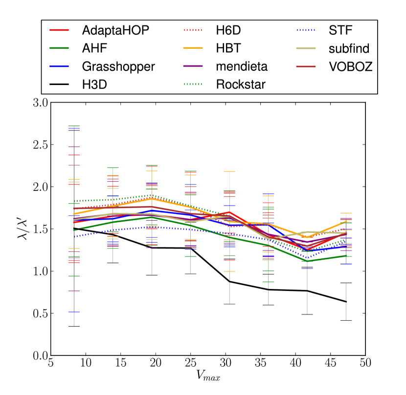
Figure 1: A comparison of the Peebles and Bullock spin parameters against $v_{\rm max}$ based on all finders using a common unbinding procedure from subhaloes with more than 300 particles. The mean value of $\lambda/\lambda^{\prime}$ is shown together with one standard deviation error bars. It shows there is a correlation between the two but not a one-to-one correspondence, with some scatter present. The scatter at low $v_{\rm max}$ where haloes have very few particles is particularly pronounced.

4 Results

The results used were restricted to subhaloes with more than 300 particles, as these produce a relatively stable value for spin. Values below this limit tend not to converge across resolutions (Bett et al., 2007).

4.1 Spin parameter

In general there is a proportional relationship between the Peebles and Bullock spin parameters recovered by all the finders for the same subhaloes, although there is some scatter as shown in Figure 1. We do not dwell on the differences between the two definitions as that has already been studied elsewhere (Hetznecker & Burkert, 2006). As both definitions of spin exist in the literature we consider both metrics when comparing how the spin is recovered across finders, placing particular emphasis on their application to subhaloes.

The majority of field haloes are found to cluster around a value of $\lambda_{0}=0.044$ for the Peebles spin parameter (Bett et al., 2007) and $\lambda_{0}^{\prime}=0.035$ for the Bullock parameter (Bullock et al., 2001) with a spread of values matched by a free parameter to give the width of the distribution.

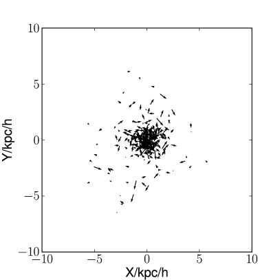
Figure 2: An example of the influence of unbinding. Left panel: particles in the object prior to unbinding. Right panel: particles in the object after unbinding the been performed. The vectors indicate the direction and velocity relative to the bulk velocity of the individual particles making up this example subhalo. The contribution from the background particles has only a minor influence on the mass and $v_{\rm max}$ of the subhalo, but a large effect on the spin parameter.

4.1.1 Spin for subhaloes with no unbinding performed

If unbinding has not been correctly implemented the high speed background particles can distort the spin parameter enormously.

To emphasise the type of structures that are found, an example of a subhalo without (left panel) and with (right panel) unbinding is shown in Figure 2. This is displayed as a vector plot of all the component particles position and velocities that make up the subhalo with the velocity vectors scaled in the same way in both panels. The bulk velocity of the subhalo has been removed and all positions and velocities are relative to the rest frame of the subhalo. Evident in the left panel of Figure 2 without unbinding are stray particles that are part of the background halo. Despite their small number these particles have both a large lever arm and large velocity relative to the halo, and significantly alter the derived value of the spin parameter due to their large angular momenta.

Comparing the two forms of the spin parameter in Figure 6 and Figure 6 we show how the spin parameter is quite chaotic, not matching a smooth Gaussian like profile as might be expected, and is clearly a long way removed from the idealised curve others have found for the distribution of spin. A significant number of the haloes have spin parameter values above 1, which is unphysical as these objects would be ripped apart by this level of rotation and so clearly cannot be equilibrium systems. This result is perhaps not surprising given the contribution from unbound background particles moving with velocities far from the mean of the object being considered but clearly shows how poor unbinding methods are relatively easy to detect by looking at the spin parameter distribution. The Peebles spin parameter is more affected by the lack of unbinding than the equivalent Bullock parameter as it takes into account the kinetic energy of all the particles. Some more objective numbers for this and subsequent comparisons are given in Table 3.

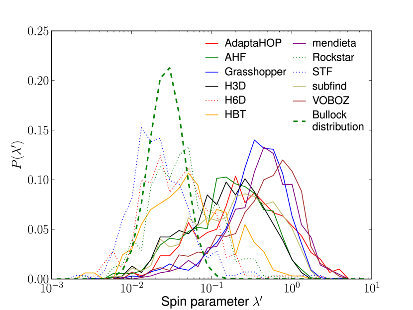
Figure 3: General profile of the Bullock spin parameter of all subhaloes found with more than 300 particles without unbinding performed, binned into 35 log bins. The results are normalised to give equal area under the visible curve. The dashed line is the field halo fit from Bullock et al. (2001). The results show a large scatter about a peak which is far distant from the fiducial fit for haloes. Dotted lines indicate finders with a phase space component of their algorithm, whereas solid lines indicate finders without a phase space component.

Figure 4: The same plot as Figure 6 but using the Peebles spin parameter and fitting function from Bett et al. (2007).

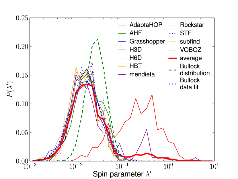
Figure 5: The same plot as Figure 6 but with the finders own unbinding processing applied to the data. This groups the spin parameters somewhat more tightly, and shows that spin is a good indicator of how well the unbinding procedure is removing spurious background particles. The adaptahop finder doesn’t perform an unbinding step, and this plot also shows up a flaw in mendieta’s unbinding procedure. The dashed line is the Bullock field halo fit curve from Bullock et al. (2001). The Bullock data fit is the best fit to the average using the Bullock fitting formula.

Figure 6: The same plot as Figure 6 except that this time the dashed line is the Peebles field halo fit from Bett et al. (2007). The Peebles best data fit is the best fit to the average of the Bett formula.

The best fit values shown by the bold dashed lines are vastly different from the fiducial values given in Section 2. It is however significant that the finders hot6d, rockstar and stf (shown by dotted lines) which all have a phase space based component in their particle collection algorithm already show a much better fit to the fiducial value than the non phase-space finders. It should be noted that when grasshopper is run without unbinding, it finds a large number of subhaloes which would normally be discarded by the unbinding procedure that is integral to the final part of the grasshopper algorithm.

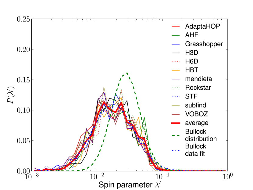
Figure 7: The same plot as Figure 6 but with a common unbinding processing applied to the data. This groups the spin parameters much more tightly, and shows that spin is a good predictor of how well the unbinding procedure performing at removing spurious background particles. The dashed line is the Bullock best fit field halo curve from Bullock et al. (2001).

Figure 8: The same plot as Figure 6 but with a common unbinding processing applied to the data. The dashed line is the Peebles best fit curve from Bett et al. (2007).

4.1.2 Spin for subhaloes with finders own unbinding performed

Including each finder’s own unbinding procedure improves the spin parameter measure considerably, as shown in Figure 6 and Figure 6. Note that as adaptahop doesn’t do any unbinding in its post-processing steps it is a clear outlier on this plot. The mendieta finder shows a double peak, which is indicative of some of the unbinding failing, an issue that the authors of the finder are currently working on.

When fitting the best fit curves to this data obtained for the spin parameter of subhaloes, the peak of the Bullock fitting curve given in Equation 4 is less than the field halo value by about 20 percent, offsetting the mean towards smaller values of the spin parameter. For the Peebles spin parameter the best fit is again offset by about 36 percent from the field halo value, again towards a smaller value of the spin parameter.

4.1.3 Spin for subhaloes with a common unbinding performed

Once a common unbinding is done, the curves move significantly closer to the idealised curve, although there is still some separation. The plots of Figure 8 and Figure 8 compare the spin parameter distribution of the different finders using a common unbinding process. It shows the match between the best fit curve quoted in Bullock et al. (2001) and Bett et al. (2007) and the haloes found by the finders taking part in the comparison. The values are now offset by 10 percent for the Bullock fit, and 30 percent for the Peebles fit. This results in the closest fit to the data, although the subhalo spin again extends to slightly lower values for both parameters, and follows the best fit line at larger values. These results also have a similar trend for the Aquarius B-E haloes and the ghalo data sets. These inclusions show that the results are not influenced greatly by the simulation, simulation engine or small changes in the cosmology used.

4.1.4 Spin at higher resolutions

Going to higher resolutions afforded by the level 1 data as shown in Figure 9, the trend to a lower spin distribution peak continues, although only three of the finders were able to manage such a computationally intensive task.

There is a more pronounced tendency to depart from the field halo fit line at low spin part of the distribution, with the peak and bulk of the distribution moving towards lower spin parameter values. The finders also show more scatter with each of them identifying the peak of the distribution in slightly different places. The agreement particularly at the low end of the spin distribution is good but with slightly lesser agreement at the high end.

Although ahf appears to find slightly more higher spin haloes, this is a result of the spherical unbinding algorithm it uses, which tends to also increase the spin distribution of the other finders slightly when used as the common unbinding procedure.

The dashed line representing the level 4 data is included to allow a direct comparison between the level 4 and level 1 average fits. It shows the continued movement of the distribution towards lower spin values with higher resolution and an increase in data.

4.1.5 Spin distribution summary

The best fit curve figures for all these plots are summarised in Table 3. Even after cleaning the catalogues significantly by utilising a common unbinding procedure for all finders there remains a definite trend for substructure spin to be less than that found for field haloes. We investigate the reason for this in the next sections.

Table 3: Summary of the best fit parameters for the graphs shown. Shown are the values for $\lambda_{0}$ and the other free parameter ($\alpha$ or $\sigma$) used in the best fit, and their difference from the published field halo fit value. The subscripts F, N, O and C are for field haloes, no unbinding, own unbinding and common unbinding respectively. The $\Delta$ values are the difference from the field halo values, and the change is the percentage difference. All results are for level 4 data except the last which is level 1

Plot	$\lambda_{0}$	$\Delta\lambda_{0}$	change	$\sigma/\alpha$	$\Delta\sigma/\alpha$	change
BullockF	0.035			0.5
PeeblesF	0.044			2.509
BullockN	1.646	1.611	+4600%	1.36	0.86	172%
PeeblesN	12.6	12.573	+29000%	41	39.2	1560%
BullockO	0.028	-0.007	-20%	0.727	0.227	45.5%
PeeblesO	0.028	-0.016	-36%	3.643	1.134	45.2%
BullockC	0.031	-0.004	-10.4%	0.75	0.25	50.0%
PeeblesC	0.03	-0.013	-30%	3.96	1.448	57.7%
Bullock-L1O	0.022	-0.013	-38%	0.693	0.193	38.6%

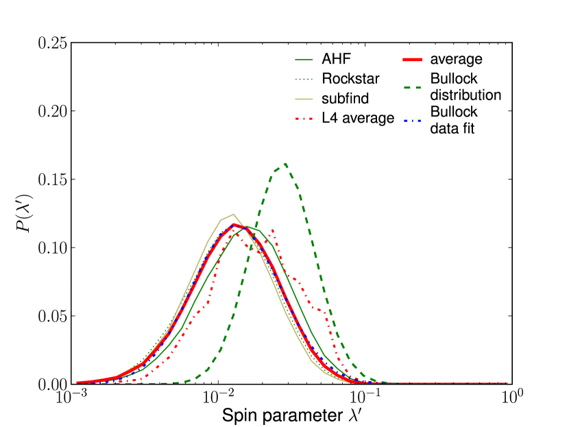
Figure 9: The same plot as Figure 6 but using the level 1 data which has much higher resolution. The lower spin haloes are more obvious in this plot, as is the difference between finders. The level 4 average is included for comparison.

4.2 Host halo radial comparison

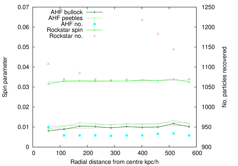
Figure 10: The spin parameter as recovered by ahf (Peebles and Bullock) and rockstar (Peebles) of an outer subhalo repositioned progressively closer to the centre. The finders own spin calculations were used in this case rather than the full pipeline. The spin is seen to be approximately unchanging across the radius.

Next we consider whether the location of a subhalo within a host halo has any effect on the recovered spin parameter. First we demonstrate in Figure 10 that any effect is not an artefact of the finding process. Substructures closer into the centre of the host halo are more difficult to detect particularly by some finders, and therefore subject to a loss of constituent particles that could be attached to the subhalo as shown in Muldrew et al. (2011). To test this supposition we took a subhalo found in the outskirts of the Aquarius-A main halo, and repositioning it at points closer to the location of the centre of the halo. Then two of the finders (ahf and rockstar) were rerun on the new data and the spin value calculated anew. The results shown in Figure 10 indicate that there is little change in the value of the spin parameter with radius despite some variation in the recovered number of particles.

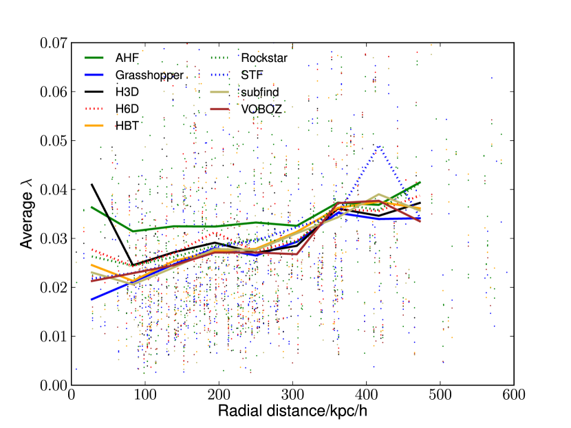
Figure 11: Comparison of mean spin parameter against radius from the centre of the host halo. Common unbinding was applied in the pipeline in this case. There is some additional scatter at low radial values as few haloes above 300 particles are found there. The background points indicate the measured spin parameter for individual subhaloes.

Next we look at whether the mean value of the measured spin parameters changes with respect to the distance from the centre of the host halo. Figure 11 displays this radial dependence for the indicated finders after a common unbinding step has been applied. The background points indicate the scatter in the spin parameter for any individual halo, as seen in the previous section. This shows a small trend for a lower mean spin as the subhaloes get closer to the centre of the host halo. This confirms the result that were found in Reed et al. (2004) but is shown here at higher resolution and across more finders than the earlier paper.

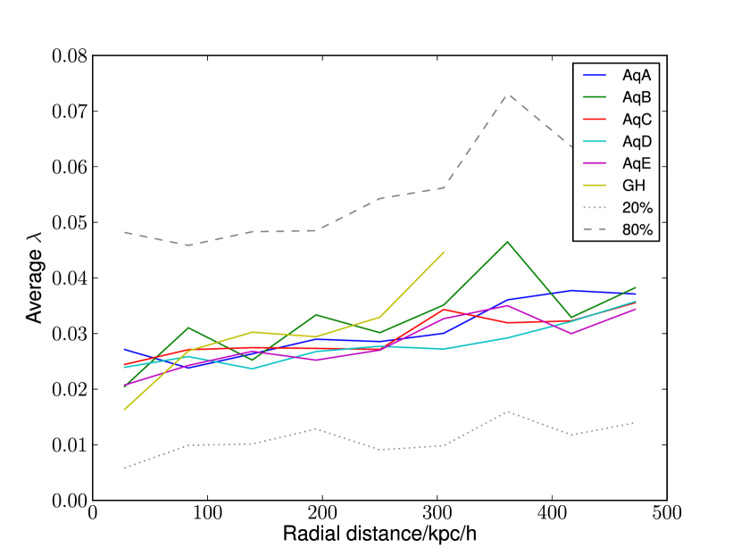
Figure 12: Comparison of mean spin parameter against radius from the centre of the host halo for several different haloes. The finders own unbinding procedure was used in the pipeline in this case. Each line is the average of the spin parameter binned into 10 bins across all finders partaking (ahf, grasshopper, rockstar, subfindand stf). The haloes used were the Aquarius-A to E and ghalo all at level 4 of the resolution. The dashed/dotted lines indicate 20 and 80 maximum percentiles across all data.

Equivalent results are found when we compare 6 different simulations generated by two different N-body codes and aggregate the average of the different finders across multiple haloes in Figure 12. This effect (as noted in Reed et al. 2004) is difficult to detect observationally, as most substructure will form galaxies before falling in so will have its spin detectable from observations of galactic rotation curve already fixed (Kauffmann et al., 1993). The possible exception to this are galaxies forming at high redshift where the infalling substructure has not yet formed stars, such as gas-rich dark galaxies (Cantalupo et al., 2012), made entirely of dark matter and gas, which may form structure after falling into a parent halo.

4.3 Build up of the spin parameter within a subhalo

This leads to the question of what causes the drop in the measured spin parameter with proximity to the centre of the host halo. Figure 13 shows the average change in the measured spin parameter as the detected subhalo is analysed from the centre outwards to its radius. This procedure is computed after the common processing and unbinding steps have been done. The subhaloes analysed in this way are then further binned into radial bins determined from the centre of the host halo. The outermost subhaloes, which are the least disrupted, show an initial decrease in measured spin parameter as particles are removed from their outer edges. Subhaloes extracted from nearer the centre of the host halo do not show this initial decrease but instead have a monotonically rising spin parameter as material is removed.

This trend suggest that subhaloes are preferentially stripped of high angular momentum particles which are likely to be the most weakly bound particles, leading to a decrease in the spin parameter as they enter the host halo. The outermost particles are usually those least bound so are the most likely to be removed on infall.

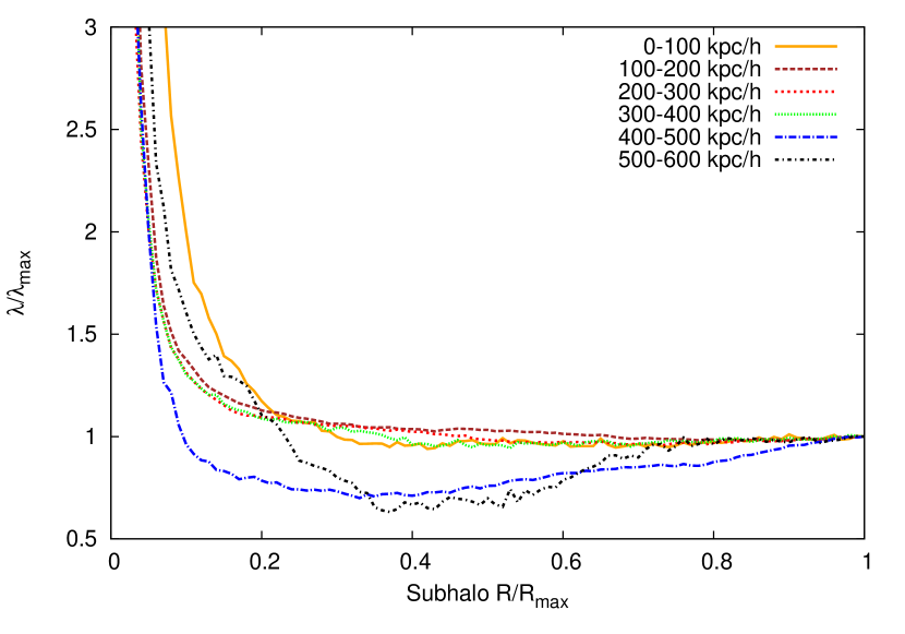
Figure 13: The radial profile of the spin parameter across the the subhalo. This shows the change in the measured spin parameter as spin is analysed from the centre to the radius of the subhalo. Here $R_{max}$ is the subhaloes maximum radius. Each line represents a different host halo radial bin. Subhaloes near the centre of the host halo show monotonically rising spin parameter values spin, whereas further out the spin parameter initially drops before rising.

We can also examine how the spin parameter is built up as mass is added to a subhalo. In Figure 14 we look at how the spin parameter changes at various mass cuts of the subhalo, $M(<M_{tot})$. This shows how the spin is built up across the structure of the subhalo. For each halo we calculate the spin parameter at 0.25, 0.5, 0.75, 0.95 of the subhalo’s total mass for all the contributing halo finders. We plot the mean and the standard deviation at each mass cut.

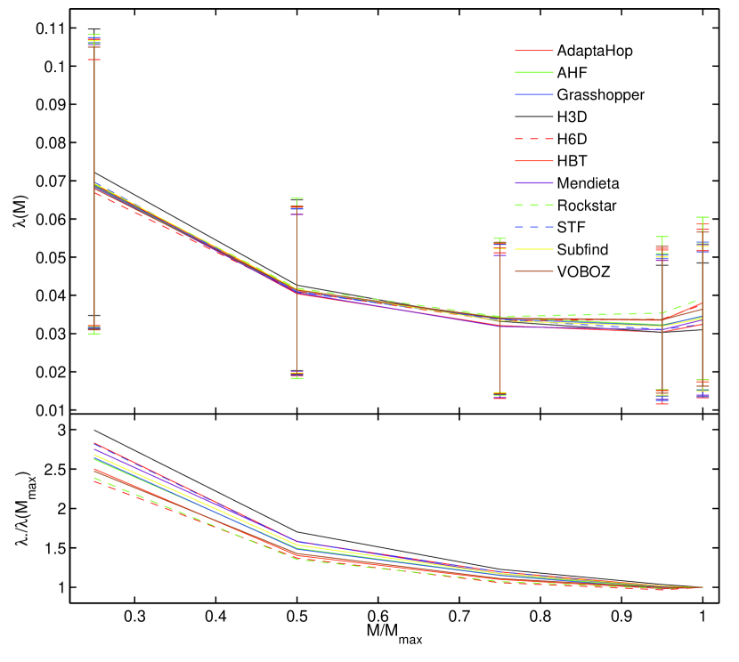
Figure 14: Comparison of the normalised mean Peebles spin at different mass shells of all subhaloes. The cuts were taken at 0.25, 0.5, 0.75, 0.95 and the complete mass of the subhalo. A common unbinding procedure was run on the results. There is a clear decrease in spin with increasing contained mass, and about a 3-fold drop is evident. The top plot shows the value of the spin parameter, and the bottom plot the spin parameter normalised to the value of $\lambda$ at the subhaloes $R_{max}$. Error bars are one standard deviation.

As expected from Figure 13 all finders agree that the calculated spin increases as the fraction of the subhalo mass that is used to calculate the spin parameter is reduced. Note that haloes have steeply rising density profiles and so the inner $50\%$ of the mass is contained within a much smaller fraction of the radius and that this result is averaged over all the recovered haloes and not split in radial bins.

5 Summary & Conclusions

There is a good level of agreement amongst the finders on the recovery of the distribution of the spin of subhaloes, although differences are still evident, causing scatter in some of the comparisons. Undoubtedly some of the scatter is due to different types of subhalo that are being recovered by the finders, some finders focusing on stream like structures and some on simple overdensities. There is still some room for improvement of the finders as the common unbinding test shows. Some of the possible improvements and sources of error will be outlined in Knebe et al. (in prep).

The distribution of spin provides a very good indicator of the finders unbinding ability and seems broadly unaffected by the cosmology and simulation engine in use. As such, the spin distribution serves as a mechanism to detect if substructure finders are performing the unbinding correctly. The unbinding errors can be masked in other comparisons such as $v_{\rm max}$ and mass plots but show up in an obvious way when the spin distribution is examined. Phase-space finders are less sensitive to poor unbinding as they have some implicit unbinding in their selection criteria when looking at velocity components. Indeed Hetznecker & Burkert (2006) and D’Onghia & Navarro (2007) both show there is a good correlation between the virialisation of haloes and the spin parameter, thus indicating its use for the determination of how relaxed the halo is, which is not unrelated to the unbinding process.

The mean spin parameter of subhaloes decreases as they approach the host halo’s centre. This is a real effect and not an artefact of any difficulty in recovering structure as the subhalo approaches the centre of the main halo. This effect is apparent in the spin parameter distribution which matches that of field haloes at larger radii but has a broader width than other published fits, extending to lower spin values. This difference between the spin properties of subhaloes and field haloes needs to be taken into account if precise measurement of the spin parameter distribution are to be made.

The recovered spin parameter goes through a minimum for subhaloes near the edge of the host at about half the $r_{\rm max}$ value. Here, if outer particles are stripped tidally as a substructure falls into a host halo, the result will be a decrease in the spin. This implies a radial dependant factor needs to be taken into account when compiling substructure catalogues, as the infalling haloes tend to have their outer particles removed. Once the outer layer has been lost the spin parameter generally increases to smaller radii as less and less mass is considered.

The value of the spin parameter measured is dependent upon the choice of where to place the outer edge and precisely which material is included in the calculation. As we have shown here and elsewhere these choices are very halo finder dependent and so care should be taken when inter-comparing spin parameter measurements from different codes.

In a future project we plan to look more closely at the difference between field and substructure haloes, to compare more directly the spin parameter found.

References

- Abadi et al. (2003) Abadi M. G., Navarro J. F., Steinmetz M., Eke V. R., 2003, The Astrophysical Journal, 591, 499
- Antonuccio-Delogu et al. (2010) Antonuccio-Delogu V., Dobrotka A., Becciani U., Cielo S., Giocoli C., Macciò A. V., Romeo-Veloná A., 2010, MNRAS, 407, 1338
- Ascasibar (2010) Ascasibar Y., 2010, Comput. Phys. Commun., 181, 1438
- Ascasibar & Binney (2005) Ascasibar Y., Binney J., 2005, MNRAS, 356, 872
- Aubert et al. (2004) Aubert D., Pichon C., Colombi S., 2004, MNRAS, 352, 376
- Barnes & Efstathiou (1987) Barnes J., Efstathiou G., 1987, ApJ, 319, 575
- Behroozi et al. (2011) Behroozi P. S., Wechsler R. H., Wu H.-Y., 2011, ArXiv preprint arXiv:1110.4372
- Benson (2012) Benson A. J., 2012, New Astronomy, 17, 175
- Benson et al. (2001) Benson A. J., Pearce F. R., Frenk C. S., Baugh C. M., Jenkins A., 2001, MNRAS, 320, 261
- Bertone et al. (2007) Bertone S., De Lucia G., Thomas P. A., 2007, MNRAS, 379, 1143
- Bett et al. (2007) Bett P., Eke V., Frenk C. S., Jenkins A., Helly J., Navarro J., 2007, MNRAS, 376, 215
- Bett et al. (2010) Bett P., Eke V., Frenk C. S., Jenkins A., Okamoto T., 2010, MNRAS, 404, 1137
- Bower et al. (2006) Bower R. G., Benson A. J., Malbon R., Helly J. C., Frenk C. S., Baugh C. M., Cole S., Lacey C. G., 2006, MNRAS, 370, 645
- Bryan et al. (2012) Bryan S. E., Kay S. T., Duffy A. R., Schaye J., Dalla Vecchia C., Booth C. M., 2012, ArXiv preprint arXiv:1207.4555
- Bullock et al. (2001) Bullock J. S., Dekel A., Kolatt T. S., Kravtsov A. V., Klypin A. A., Porciani C., Primack J. R., 2001, ApJ, 555, 240
- Cantalupo et al. (2012) Cantalupo S., Lilly S. J., Haehnelt M. G., 2012, MNRAS, 425, 1992
- Cole et al. (2000) Cole S., Lacey C. G., Baugh C. M., Frenk C. S., 2000, MNRAS, 319, 168
- Croton et al. (2006) Croton D. J., Springel V., White S. D. M., De Lucia G., Frenk C. S., Gao L., Jenkins A., Kauffmann G., Navarro J. F., Yoshida N., 2006, MNRAS, 365, 11
- Dalcanton et al. (1997) Dalcanton J. J., Spergel D. N., Summers F. J., 1997, ApJ, 482, 659
- De Lucia & Blaizot (2007) De Lucia G., Blaizot J., 2007, MNRAS, 375, 2
- D’Onghia & Navarro (2007) D’Onghia E., Navarro J. F., 2007, MNRAS, 380, L58
- Eisenstein & Hut (1998) Eisenstein D. J., Hut P., 1998, ApJ, 498, 137
- Elahi et al. (2011) Elahi P. J., Thacker R. J., Widrow L. M., 2011, MNRAS, 418, 320
- Fall & Efstathiou (1980) Fall S., Efstathiou G., 1980, MNRAS, 193, 189
- Font et al. (2008) Font A. S., Bower R. G., McCarthy I. G., Benson A. J., Frenk C. S., Helly J. C., Lacey C. G., Baugh C. M., Cole S., 2008, MNRAS, 389, 1619
- Frenk & White (2012) Frenk C., White S., 2012, Annalen der Physik, 524, 507
- Frenk et al. (1997) Frenk C. S., Baugh C. M., Cole S., Lacey S., 1997, in Persic M., Salucci P., eds, Dark and Visible Matter in Galaxies and Cosmological Implications Vol. 117 of Astronomical Society of the Pacific Conference Series, Numerical and Analytical Modelling of Galaxy Formation and Evolution. p. 335
- Gill et al. (2004) Gill S. P., Knebe A., Gibson B. K., 2004, MNRAS, 351, 399
- Gottlöber & Yepes (2007) Gottlöber S., Yepes G., 2007, ApJ, 664, 117
- Han et al. (2011) Han J., Jing Y. P., Wang H., Wang W., 2011, Arxiv preprint arXiv:1103.2099
- Hetznecker & Burkert (2006) Hetznecker H., Burkert A., 2006, MNRAS, 370, 1905
- Jarosik et al. (2011) Jarosik N., Bennett C. L., Dunkley J., Gold B., Greason M. R., Halpern M., Hill R. S., Hinshaw G., Kogut A., Komatsu E., Larson D., Limon M., Meyer S. S., Nolta M. R., Odegard N., Page L., Smith K. M., Spergel D., Tucker G. S., Weiland J. L., Wollack E., Wright E. L., 2011, ApJS, 192, 14
- Kauffmann et al. (1997) Kauffmann G., Nusser A., Steinmetz M., 1997, MNRAS, 286, 795
- Kauffmann et al. (1993) Kauffmann G., White S. D. M., Guiderdoni B., 1993, MNRAS, 264, 201
- Knebe et al. (2011) Knebe A., Knollmann S. R., Muldrew S. I., Pearce F. R., Aragon-Calvo M. A., Ascasibar Y., Behroozi P. S., Ceverino D., Colombi S., Diemand J., 2011, MNRAS, pp 819–
- Knebe & Power (2008) Knebe A., Power C., 2008, ApJ, 678, 621
- Knollmann & Knebe (2009) Knollmann S. R., Knebe A., 2009, ApJS, 182, 608
- Lacerna & Padilla (2012) Lacerna I., Padilla N., 2012, MNRAS, 426, L26
- Macciò et al. (2007) Macciò A. V., Dutton A. A., Van Den Bosch F. C., Moore B., Potter D., Stadel J., 2007, MNRAS, 378, 55
- Mestel (1963) Mestel L., 1963, MNRAS, 126, 553
- Mo et al. (1998) Mo H. J., Mao S., White S. D. M., 1998, MNRAS, 295, 319
- Muldrew et al. (2011) Muldrew S. I., Pearce F. R., Power C., 2011, MNRAS, 410, 2617
- Navarro & Steinmetz (2000) Navarro J. F., Steinmetz M., 2000, ApJ, 538, 477
- Neyrinck et al. (2005) Neyrinck M. C., Gnedin N. Y., Hamilton A. J. S., 2005, MNRAS, 356, 1222
- Onions et al. (2012) Onions J., Knebe A., Pearce F. R., Muldrew S. I., Lux H., Knollmann S. R., Ascasibar Y., Behroozi P., Elahi P., Han J., Maciejewski M., Merchán M. E., Neyrinck M., Ruiz A. N., Sgró M. A., Springel V., Tweed D., 2012, MNRAS, 423, 1200
- Peebles (1969) Peebles P., 1969, ApJ, 155, 393
- Read et al. (2010) Read J. I., Hayfield T., Agertz O., 2010, MNRAS, 405, 1513
- Reed et al. (2004) Reed D., Governato F., Quinn T., Gardner J., Stadel J., Lake G., 2004, MNRAS, 359, 1537
- Sgró et al. (2010) Sgró M. A., Ruiz A. N., Merchán M. E., 2010, BAAA, 53, 43
- Springel (2005) Springel V., 2005, MNRAS, 364, 1105
- Springel et al. (2008) Springel V., Wang J., Vogelsberger M., Ludlow A., Jenkins A., Helmi A., Navarro J. F., Frenk C. S., White S. D., 2008, MNRAS, 391, 1685
- Springel et al. (2005) Springel V., White S. D. M., Jenkins A., Frenk C. S., Yoshida N., Gao L., Navarro J., Thacker R., Croton D., Helly J., Peacock J. A., Cole S., Thomas P., Couchman H., Evrard A., Colberg J., Pearce F., 2005, Nat, 435, 629
- Springel et al. (2001) Springel V., White S. D. M., Tormen G., Kauffmann G., 2001, MNRAS, 328, 726
- Stadel (2001) Stadel J., 2001, PhD thesis, University of Washington
- Stadel et al. (2009) Stadel J., Potter D., Moore B., Diemand J., Madau P., Zemp M., Kuhlen M., Quilis V., 2009, MNRAS, 398, L21
- Stadel et al. (2002) Stadel J., Wadsley J., Richardson D., , 2002, High performance computational astrophysics with pkdgrav/gasoline
- Trowland et al. (2012) Trowland H. E., Lewis G. F., Bland-Hawthorn J., 2012, ArXiv preprint arXiv:1201.6108
- Tweed et al. (2009) Tweed D., Devriendt J., Blaizot J., Colombi S., Slyz A., 2009, A&A, 506, 647
- Vitvitska et al. (2002) Vitvitska M., Klypin A. A., Kravtsov A. V., Wechsler R. H., Primack J. R., Bullock J. S., 2002, The Astrophysical Journal, 581, 799
- Wang et al. (2011) Wang H., Mo H. J., Jing Y. P., Yang X., Wang Y., 2011, MNRAS, 413, 1973
- White & Frenk (1991) White S., Frenk C., 1991, ApJ, 379, 52
- White (1984) White S. D. M., 1984, ApJ, 286, 38
- White & Rees (1978) White S. D. M., Rees M. J., 1978, MNRAS, 183, 341