Laser-induced effects on the electronic features of graphene nanoribbons

Abstract

We study the interplay between lateral confinement and photon-induced processes on the electronic properties of illuminated graphene nanoribbons. We find that by tuning the device setup (edges geometries, ribbon width and polarization direction), a laser with frequency $\Omega$ may either not affect the electronic structure, or induce bandgaps or depletions at $\pm\hbar\Omega/2$, and/or at other energies not commensurate with half the photon energy. Similar features are also observed in the dc conductance, suggesting the use of the polarization direction to switch on and off the graphene device. Our results could guide the design of novel types of optoelectronic nano-devices.

The extraordinary properties of graphene Geim2009 ; CastroNeto2009 ; Dubois2009 led to an unprecedented narrowing in the expected gap between the understanding of new phenomena and the development of disruptive applications Geim2009 . Though originally focused mainly on pure electronic, mechanical or optical properties, much attention is now devoted to the interplay between these variables Bonaccorso et al. (2010). Graphene optoelectronics Bonaccorso et al. (2010); Xia et al. (2009); Gabor et al. (2011); Karch et al. (2011); Koppens et al. (2011); Ren2009 ; McIver2012 , in particular, is one of the most active and promising fields with flagship applications including energy harvesting devices Gabor et al. (2011) and novel plasmonic properties Koppens et al. (2011); Chen2012 .

Recently, the captivating possibility of controlling the electronic properties of graphene through simple illumination with a laser field Syzranov et al. (2008); Oka and Aoki (2009) has been re-examined through atomistic calculations Calvo et al. (2011), calculations of the optical response Zhou and Wu (2011); Busl et al. (2012) and proposals for tuning the topological properties of the underlying photon-induced states Kitagawa et al. (2011); Gu et al. (2011); Dóra et al. (2012); Suarez Morell and Foa Torres (2012), among other interesting issues Abergel and Chakraborty (2009); Kibis (2010); Savel’ev and Alexandrov (2011); Iurov et al. (2012); Liu et al. (2012); San-Jose et al. . The basic idea is that laser illumination may couple states on each side of the charge neutrality point inducing a bandgap at $\pm\hbar\Omega/2$, if the field intensity and frequency are appropriately tuned. This non-adiabatic and non-perturbative effect relies crucially on the low dimensionality and peculiar electronic structure of graphene and has attracted much recent attention Kitagawa et al. (2011); Gu et al. (2011); Dóra et al. (2012); Suarez Morell and Foa Torres (2012). Notwithstanding, most of these predictions were restricted to bulk graphene. One may wonder about the possible consequences of reduced dimensionality and quantum confinement.

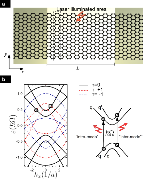
Figure 1: (Color online) $a$- Scheme of the considered setup: A graphene nanoribbon illuminated by a mid-infrared laser within a finite region of length $L$. The unit cell for the case of an armchair ribbon is marked with a rectangle (dashed line) and contains $4N$ atoms in the notation used in the text. $b$- Floquet quasi-energy dispersion for a small ribbon ($N=2$). For the sake of better visualization, we show the quasi-energy spectrum without radiation (this allows to better distinguish the crossings between levels) and choose arbitrary frequency and intensity values. More realistic results are shown in Figs. 2 and 3. The scheme on the right shows the electronic states for two of such transitions.

Here, we address the effects of laser illumination on graphene nanoribbons and show that lateral confinement plays a crucial role: tuning the sample size and the direction between the laser polarization relative to the sample edges, linearly polarized light may or not induce bandgaps or depletions in the density of states and the conductance spectra. Strikingly, for finite size samples these features may appear at energies different from integer multiples of $\pm\hbar\Omega/2$. This is in stark contrast with bulk graphene where the electrical response is insensitive to the linear polarization direction. Our results fill the gap in the understanding of the laser-induced control of the electrical response and may guide the design of new experiments on optoelectronic devices.

Hamiltonian model and solution scheme. We consider an infinite graphene nanoribbon illuminated by a laser only in a finite region of length $L$ and perpendicular to it (as shown schematically in Fig. 1-$a$). Electrons in the graphene ribbon are modeled through a nearest neighbours $\pi$-orbitals Hamiltonian Dubois2009 ; SaitoBook : $H_{e}=\sum_{i}E_{i}c_{i}^{+}c_{i}-\sum_{\left\langle i,j\right\rangle}[\gamma_{i,j}c_{i}^{+}c_{j}+\mathrm{H.c.}]$, where $c_{i}^{+}$ and $c_{i}$ are the electronic creation and annihilation operators at site $i$, $E_{i}$ are the on-site energies and $\gamma_{i,j}$ the nearest-neighbors carbon-carbon hoppings amplitudes which are taken equal to $\gamma_{0}=2.7\,\mathrm{eV}$ Dubois2009 . Radiation is described through a time-dependent electric field $\mathbf{E}$. By choosing a gauge such that $\mathbf{E}=-\partial\mathbf{A}/\partial t$, where $\mathbf{A}$ is the vector potential, the hopping matrix elements acquire a time-dependent phase according to: $\gamma_{ij}=\gamma_{0}\exp\left(\mathrm{i}\frac{2\pi}{\Phi_{0}}\int_{\mathbf{r}_{i}}^{\mathbf{r}_{j}}\mathbf{A}(t)\cdot\mathrm{d}\mathbf{r}\right)$, where $\Phi_{0}$ is the magnetic flux quantum.

Retaining non-perturbative and non-adiabatic corrections to the electrical response is crucial for the results presented hereafter. In this regime, Floquet theory provides an appropriate framework. An efficient solution using this scheme is used to obtain the average density of states and the dc component of the conductance, which is computed from the inelastic transmission probabilities in Floquet space Kohler et al. (2005). The interested reader may find further generalities of the method in Refs. Kohler et al. (2005); Foa Torres (2005), while more technical details will be published elsewhere JPCM2012 . For a periodic modulation of the hoppings, the spectral and transport properties can be derived from the so-called Floquet Hamiltonian: $H_{F}=H_{e}-i\hbar\partial/\partial t$. Such Hamiltonian has a time-independent representation in the Floquet space, which is the direct product between the usual Hilbert space and the space of time-periodic functions with the same period as the Hamiltonian $H_{e}$ Shirley ; Kohler et al. (2005). Therefore, on top of the $k$ label, our states have a second label which indicates the number $n$ of photon excitations in the system. In the absence of radiation, the quasi-energies spectrum of $H_{F}$ are given by $\varepsilon(\mathbf{k},n)=\varepsilon_{0}(\mathbf{k})+n\hbar\Omega$ ($\varepsilon_{0}(\mathbf{k})$ is the spectrum of $H_{e}$).

Electronic properties of irradiated graphene nanoribbons. The first question we address is whereas the response of graphene nanoribbons to a laser is sensitive to the (linear) polarization direction. While in the bulk limit both the conductance and the density of states are independent on the polarization direction, the picture turns out to change radically in confined geometries.

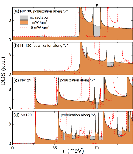
Figure 2: (Color online) Average density of states for armchair graphene nanoribbons with $N=130$ ($a$,$b$) and $N=129$ ($c$,$d$) for two values of the laser power $P$: $1\,\mathrm{mW/\mu m^{2}}$ (solid black line with orange shaded area) and $10\,\mathrm{mW/\mu m^{2}}$ (dotted red line). Panels $a$ and $c$ ($b$ and $d$) are for polarization along the $x$ direction ($y$ direction). The energy corresponding to $\hbar\Omega/2$ is marked with an arrow for reference in the top of the panel. The DOS in absence of radiation is also shown for comparison (dashed lines, grey shaded area).

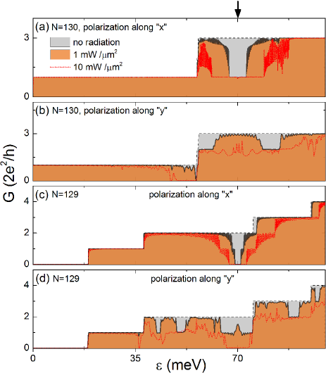
Figure 3: (Color online) DC conductance for armchair graphene nanoribbons with $N=130$ ($a$,$b$) and $N=129$ ($c$,$d$). Panels $a$ and $c$ ($b$ and $d$) are for polarization along the $x$ direction ($y$ direction).

Figure 2 shows the average density of states as a function of the Fermi energy for a frequency in the mid-infrared regime ($\hbar\Omega=140\,\mathrm{meV}$). Two different armchair nanoribbons sizes and polarizations are chosen: $N=130$ ($a$ and $b$), $N=129$ ($c$ and $d$); and linear polarization along the $x$ ($a$ and $c$) and $y$ ($b$ and $d$) directions. For $N=130$ one sees the appearance of strong depletions at $\pm\hbar\Omega/2$. These depletions are located at the same energy as the ones for the bulk system Calvo et al. (2011) and correspond to the excitation of an electron between the conjugate states at $\pm\hbar\Omega/2$. In striking contrast, the DOS is restored at $\pm\hbar\Omega/2$ for y-polarized laser, whereas new features occur at energies incommensurate with $\hbar\Omega$.

The DOS for the ribbon with $N=129$ ($c$ and $d$) also exhibit a laser-induced fragmentation of the spectrum, with in this case the observation of fully depleted energy regions (bandgap) at $\pm\hbar\Omega/2$. One observes that by increasing the laser intensity, some DOS modifications are further enhanced (see for instance the DOS depletion around $\hbar\Omega/2$ for Fig. 2-$a$), complemented by the emergence of new fine structure. Figure 3 shows the dc conductance as a function of the Fermi energy position for the same cases shown in Fig. 2. Here, we see that the depletions in the DOS have the same conductance fingerprints. One can see that switching the polarization direction may produce a marked on-off ratio if the Fermi energy is appropriately tuned.

To rationalize these differences, it is instructive to write $H_{e}$ in a basis of independent transversal channels or modes as discussed in Refs. Rocha et al. (2010); Zhao and Guo (2009). In the absence of radiation, the Floquet spectrum of the system is just the sum of the contributions from each of the modes $\varepsilon_{0}(\mathbf{k})$ plus their Floquet replicas: $\varepsilon(\mathbf{k},n)=\varepsilon_{0}(\mathbf{k})+n\hbar\Omega$. An illustration for a very small system is shown in Fig. 1-$b$, each mode contains an electron and a hole branch. At the crossings between the different lines, one may expect for the effects of radiation to be stronger (if it provides the necessary coupling between the corresponding states).

From the Floquet spectrum in Fig. 1-$b$ one can see that there are two kind of crossings: the ones that connect an electronic (hole) state with a hole (electron) state belonging to the same mode plus or minus an integer number of photons (like the one marked with an open circle); and the ones that connect states in different modes (as the one marked with an open square in Fig. 1-$b$). In such cases, a non-vanishing matrix element of the Floquet Hamiltonian will give intra and inter-mode transitions respectively. Given the electron-hole symmetry of the spectrum, intra-mode transitions always connect states which are symmetric relative to the Dirac point, i.e. integer multiples of $\pm\hbar\Omega/2$. On the other hand, inter-mode transitions always couple states which are not symmetrically located from the Dirac point, as can be seen on Fig. 1-$b$. A scheme showing these two type of transitions is shown in Fig. 1-$b$.

For armchair graphene nanoribbons, it turns out that a laser with linear polarization along the transport direction ($x$) does not mix these transversal modes, leading to features in the density of states only at $\pm n\hbar\Omega/2$ as can be seen in Fig. 1-$b$. On the other hand, calculation of the matrix elements shows that when the polarization is along $y$, inter-mode processes are allowed and intra-mode ones are forbidden. Depletions or gaps appear now at the crossing between Floquet states corresponding to different modes leading to the features observed in Fig. 2-$b$ and $c$.

A complementary approach to this problem is possible by using the k.p model, which could be accurate enough for medium-sized ribbons Brey . A careful analysis shows consistent results: inter-mode processes lead to gaps/depletions located away from $\pm\hbar\Omega/2$ while polarization along $y$ suppresses the depletions at $\pm\hbar\Omega/2$. In the bulk limit, as the energy difference between subbands gets smaller, the crossings between Floquet states accumulate close to $\pm\hbar\Omega/2$ leading to the same behavior for both polarizations (along $x$ and $y$). A flavor of this can be seen in the red dotted lines in Fig. 2-$b$ and $c$: The two depletions seen in Fig. 2-$d$ black line merge when increasing the laser power.

Another interesting feature is that the metallic modes/subbands in armchair ribbons are quite insensitive to the radiation (as seen in Figs. 2 and 3). Hence, very small metallic armchair ribbons containing only one transport channel within the energy range of interest will not experience relevant changes in their electronic properties. We emphasize that this is a peculiar property of armchair graphene nanoribbons JPCM2012 .

Figures 2 and 3 correspond to a laser frequency in the mid-infrared, which gives an optimum playground to test these predictions in the laboratory. Going to higher frequencies may help to achieve device miniaturization but the size of the gaps and depletions at constant laser power diminishes, whereas at very low frequencies (THz) the gaps further decrease. Experiments would require temperatures below $20\,\mathrm{K}$ for $P\simeq 1\,\mathrm{mW/\mu m^{2}}$.

In summary, we show that the interplay between photon-induced inelastic processes and lateral confinement in graphene nanoribbons leads to diverse modifications in the band structure and transport properties not evident in the bulk limit. In the case of moderate sized nanoribbons (ca. $10\,\mathrm{nm}$), the careful tuning of the polarization direction may widen the opportunities for achieving control of the electrical response in optoelectronic devices.

Acknowledgments. We acknowledge support by SeCyT-UNC, ANPCyT-FonCyT (Argentina). LEFFT acknowledges the support from the Alexander von Humboldt Foundation and ICTP-Trieste, as well as discussions with G. Usaj.

References

- (1) A. K. Geim, Science 324, 1934 (2009); A. K. Geim and K. S. Novoselov, Nat. Mat. 6, 183 (2007).
- (2) A. H. Castro Neto, F. Guinea, N. M. R. Peres, K. S. Novoselov and A. K. Geim, Rev. Mod. Phys. 81, 109 (2009).
- (3) S.M.-M. Dubois, Z. Zanolli, X. Declerck, and J.-C. Charlier, Eur. Phys. J. B 72, 1 (2009); J.-C. Charlier, X. Blase, and S. Roche, Rev. Mod. Phys. 79, 677 (2007).
- Bonaccorso et al. (2010) F. Bonaccorso, Z. Sun, T. Hasan, and A. C. Ferrari, Nat Photon 4, 611 (2010).
- Xia et al. (2009) F. Xia, T. Mueller, Y.-m. Lin, A. Valdes-Garcia, and P. Avouris, Nat Nano 4, 839 (2009).
- Gabor et al. (2011) N. M. Gabor, J. C. W. Song, Q. Ma, N. L. Nair, T. Taychatanapat, K. Watanabe, T. Taniguchi, L. S. Levitov, and P. Jarillo-Herrero, Science 334, 648 (2011).
- Karch et al. (2011) J. Karch, C. Drexler, P. Olbrich, M. Fehrenbacher, M. Hirmer, M. M. Glazov, S. A. Tarasenko, E. L. Ivchenko, B. Birkner, J. Eroms, et al., Phys. Rev. Lett. 107, 276601 (2011).
- Koppens et al. (2011) F. H. L. Koppens, D. E. Chang, and F. J. García de Abajo, Nano Lett. 11, 3370 (2011).
- (9) L. Ren, C. L. Pint, L. G. Booshehri, W. D. Rice, X. Wang, D. J. Hilton, K. Takeya, I. Kawayama, M. Tonouchi, R. H. Hauge and
- (10) J. W. McIver, D. Hsieh, H. Steinberg, P. Jarillo-Herrero and N. Gedik, Nat. Nanotech. 7, 96 (2012).
- (11) J. Chen, M. Badioli, P. Alonso-Gonzalez, S. Thongrattanasiri, F. Huth, J. Osmond, M. Spasenovic, A. Centeno, A. Pesquera, Ph. Godignon, A. Zurutuza Elorza, N. Camara, F. J. Garcia de Abajo, R. Hillenbrand and F. H. L. Koppens, Nature (2012), doi:10.1038/nature11254.
- Syzranov et al. (2008) S. V. Syzranov, M. V. Fistul, and K. B. Efetov, Phys. Rev. B 78, 045407 (2008).
- Oka and Aoki (2009) T. Oka and H. Aoki, Phys. Rev. B 79, 081406 (2009).
- Calvo et al. (2011) H. L. Calvo, H. M. Pastawski, S. Roche, and L. E. F. Foa Torres, Appl. Phys. Lett. 98, 232103 (2011).
- Zhou and Wu (2011) Y. Zhou and M. W. Wu, Phys. Rev. B 83, 245436 (2011).
- Busl et al. (2012) M. Busl, G. Platero, and A.-P. Jauho, Phys. Rev. B 85, 155449 (2012).
- Kitagawa et al. (2011) T. Kitagawa, T. Oka, A. Brataas, L. Fu, and E. Demler, Phys. Rev. B 84, 235108 (2011).
- Gu et al. (2011) Z. Gu, H. A. Fertig, D. P. Arovas, and A. Auerbach, Phys. Rev. Lett. 107, 216601 (2011).
- Dóra et al. (2012) B. Dóra, J. Cayssol, F. Simon, and R. Moessner, Phys. Rev. Lett. 108, 056602 (2012).
- Suarez Morell and Foa Torres (2012) E. Suarez Morell and L. E. F. Foa Torres, Physical Review B 86, 125449 (2012).
- Abergel and Chakraborty (2009) D. S. L. Abergel and T. Chakraborty, Appl. Phys. Lett. 95, 062107 (2009).
- Kibis (2010) O. V. Kibis, Phys. Rev. B 81, 165433 (2010).
- Savel’ev and Alexandrov (2011) S. E. Savel’ev and A. S. Alexandrov, Phys. Rev. B 84, 035428 (2011).
- Iurov et al. (2012) A. Iurov, G. Gumbs, O. Roslyak, and D. Huang, Journal of Physics: Condensed Matter 24, 015303 (2012).
- Liu et al. (2012) J.-T. Liu, F.-H. Su, H. Wang, and X.-H. Deng, New Journal of Physics 14, 013012 (2012).
- (26) P. San-Jose, E. Prada, H. Schomerus, and S. Kohler, Appl. Phys. Lett. 101, 153506 (2012).
- (27) R. Saito, G. Dresselhaus, and M. S. Dresselhaus, 1998, Physical Properties of Carbon Nanotubes (Imperial College Press, London).
- Kohler et al. (2005) S. Kohler, J. Lehmann, and P. Hänggi, Physics Reports 406, 379 (2005).
- Foa Torres (2005) L. E. F. Foa Torres, Phys. Rev. B 72, 245339 (2005).
- (30) H. L. Calvo, P. Perez Piskunow, H. M. Pastawski, S. Roche, L. E. F. Foa Torres, unpublished.
- (31) J. H. Shirley, Phys. Rev. 138, B979 (1965); H. Sambe, Phys. Rev. A 7, 2203 (1973).
- (32) L. Brey, H.A. Fertig, Phys. Rev. B 73, 235411 (2006); P. Marconcini and P. Maccuci, Riv. del Nuovo Cimento 34, 489 (2011).
- Rocha et al. (2010) C. G. Rocha, L. E. F. Foa Torres, and G. Cuniberti, Phys. Rev. B 81, 115435 (2010).
- Zhao and Guo (2009) P. Zhao and J. Guo, Journal of Applied Physics 105, 034503 (2009).