Temperature-dependent classical phonons from efficient non-dynamical simulations

Abstract

We present a method to calculate classical lattice-dynamical quantities, like the temperature-dependent vibrational spectrum, from simulations that do not require an explicit solution of the time evolution. We start from the moment expansion of the relevant time-correlation function for a many-body system, and show that it can be conveniently rewritten by using a basis in which the low-order moments are diagonal. This allows us to approximate the main spectral features (i.e., position and width of the phonon peaks) from thermal averages available from any statistical simulation. We illustrate our method with an application to a model system that presents a structural transition and strongly temperature-dependent phonons. Our theory also clarifies the status of previous heuristic schemes to estimate phonon frequencies.

Is it possible to compute any equilibrium property of a material from appropriate thermal averages? From an atomistic simulation perspective, an affirmative answer to this question implies that, if we can characterize the configuration space accessible at a temperature $T$ – as can be done e.g. with Monte Carlo (MC) methods –, we can also calculate any quantity of interest. In particular, time-correlation functions would become available, which would allow us to compute non-trivial properties like $T$-dependent phonon spectra or lattice thermal-transport coefficients without explicitly solving the equations of motion. Such a non-dynamical approach would have many advantages: as in MC schemes, fixing $T$ would become trivial, and we would avoid the problems associated with the use of thermostats in molecular-dynamics (MD) simulations; there would be no need for very long MD runs to access low-frequency phenomena, etc.

In the particular case of the vibrational spectrum, several heuristic schemes have been proposed to realize such a goal. For example, Hellman et al. hellman11 compute phonons at finite $T$ from an effective dynamical matrix that they postulate and obtain in a computationally efficient way; a similar effective potential is used in Refs. brooks95, and wheeler03, to capture anharmonic effects in the vibrational spectrum; others have used the harmonic relation between a normal-mode frequency and the amplitude of its oscillations to compute dynamical properties even from powder diffraction data book-dove05 ; goodwin04 ; goodwin05 . While such methods are valuable, we have to resort to earlier works to find a rigorous and general treatment. As recognized in a variety of fields vanvleck48 ; degennes59 ; mori65 , a time-correlation function can be obtained from the knowledge of its moments, which are static quantities that can be computed from efficient statistical simulations. In the context of lattice-dynamical studies, the moment-based approach introduced by Mori mori65 ; balucani03 has been used to investigate a number of simple systems at both the quantum and classical levels cuccoli92 ; cuccoli93 ; cowley94 ; macchi96 ; balucani03 ; however, it has failed to gain popularity in the field of classical MD. As far as we can see, this is probably because (1) we lack a general scheme to tackle arbitrarily complex materials with many atoms in the cell and (2) there has not been enough work to identify the simplest approximations that may render useful results (i.e., reliable phonon frequencies and possibly peak widths). Here we present our own derivation of a moment-based formalism for the classical case, remedying the mentioned deficiencies. The resulting theory allows us to clarify the status of the heuristic methods in the literature and, in our opinion, should become a standard tool in the field of classical simulations.

General formalism.– We define the classical correlation function of quantities $A_{i}$ and $B_{j}$ as

$$C^{AB}_{ij}(t)=\langle A_{i}(0)B_{j}(t)\rangle=\int_{-\infty}^{\infty}C^{AB}_{ij}(\omega)\,e^{i\omega t}\,d\omega$$ (1)

where $\langle...\rangle$ indicates thermal averaging and $C^{AB}_{ij}(\omega)$ is the corresponding spectral function. Below we will identify $A_{i}$ and $B_{j}$ with atomic positions or velocities, $i$ and $j$ being composite indices that label an atom and a direction in space. Note that $C^{AB}_{ij}(t)$ is real, which implies $C^{AB}_{ij}(-\omega)=[C^{AB}_{ij}(\omega)]^{*}$. For simplicity, we will work with the real part $\widetilde{C}^{AA}_{ij}(\omega)$ = $\Re[C^{AA}_{ij}(\omega)]$, as this will contain the information about the vibrational spectrum fn_real_part . Thus, in the time domain we have

$$\widetilde{C}^{AA}_{ij}(t)=\int_{-\infty}^{\infty}\widetilde{C}^{AA}_{ij}(\omega)\,cos(\omega t)\,d\omega\,,$$ (2)

which is even with respect to time inversion and can be Taylor expanded in the following way

$$\widetilde{C}_{ij}^{AA}(t)=\sum_{n=0}^{\infty}\,(-1)^{n}\,\frac{\mu_{ij}^{A,2n}}{(2n!)}\,t^{2n}\,,$$ (3)

with the moments given by

$$\mu_{ij}^{A,2n}=\int_{-\infty}^{\infty}\,\omega^{2n}\,\widetilde{C}_{ij}^{AA}(\omega)\,d\omega\,.$$ (4)

The next key step is to prove that these moments can be written as certain correlation functions at $t=0$, and can thus be computed as regular thermal averages. By successive partial integration, one can see that

$$\begin{split}\widetilde{C}_{ij}^{AA}(\omega)&=\omega^{-2}\,\widetilde{C}_{ij}^{A^{(1)}A^{(1)}}(\omega)=-\omega^{-2}\,\widetilde{C}_{ij}^{A^{(2)}A}(\omega)\\ &=\frac{(-1)^{m+n}}{\omega^{2m+2n+2p}}\,\widetilde{C}^{A^{(2m+p)}A^{(2n+p)}}_{ij}(\omega)\,,\end{split}$$ (5)

where $A^{(n)}_{i}$ is the $n$-th time derivative of $A_{i}$. These identities allow us to rewrite Eq. (4) in different ways. From a computational viewpoint, it is convenient to use

$$\mu_{ij}^{A,2n}=\int_{-\infty}^{\infty}\widetilde{C}^{A^{(n)}A^{(n)}}_{ij}(\omega)\,d\omega=\langle A_{i}^{(n)}(0)A_{j}^{(n)}(0)\rangle\,,$$ (6)

which involves time derivatives of the lowest possible order. Finally, the derivatives can be computed using Hamilton’s equation of motion

$$\begin{split}&\frac{dA}{dt}=\frac{\partial A}{\partial t}+\{A,H\}\,,\\ &\{A,H\}=\sum_{i}\left(\frac{\partial A}{\partial x_{i}}\frac{\partial H}{\partial p_{i}}-\frac{\partial A}{\partial p_{i}}\frac{\partial H}{\partial x_{i}}\right)\,.\end{split}$$ (7)

The Hamiltonian is

$$H=\sum_{i}\frac{{p}_{i}^{2}}{2m_{i}}+V(\{x_{i}\})\,,$$ (8)

where $m_{i}$, $x_{i}$, and $p_{i}$ are mass, position and momentum, respectively, and $V$ is a velocity-independent potential. It is convenient to introduce $x_{i}^{\prime}$ = $\sqrt{m_{i}}x_{i}$ to get rid of the mass dependence in the kinetic energy. We will thus work with the moments $\mu^{A^{\prime},2n}_{ij}$ of the correlation function $\widetilde{C}_{ij}^{A^{\prime}A^{\prime}}(t)$ = $\sqrt{m_{i}m_{j}}\widetilde{C}_{ij}^{AA}(t)$, where $A_{i}^{\prime}$ = $\sqrt{m_{i}}A_{i}$. The simplest object that gives information about the vibrational spectrum is the position-position correlation function. By taking $A_{i}^{\prime}$ = $\bar{x}_{i}^{\prime}$ = $x_{i}^{\prime}-\langle x_{i}^{\prime}\rangle$, we obtain

$$\begin{split}\mu^{\bar{x}^{\prime},0}_{ij}&=\sqrt{m_{i}m_{j}}\,\left(\langle x_{i}x_{j}\rangle-\langle x_{i}\rangle\langle x_{j}\rangle\right)\,,\\ \mu^{\bar{x}^{\prime},2}_{ij}&=\beta^{-1}\delta_{ij}\,,\\ \mu^{\bar{x}^{\prime},4}_{ij}&=\frac{1}{\sqrt{m_{i}m_{j}}}\,\left\langle\frac{\partial V}{\partial x_{i}}\frac{\partial V}{\partial x_{j}}\right\rangle\,,\\ \mu^{\bar{x}^{\prime},6}_{ij}&=\frac{\beta^{-1}}{\sqrt{m_{i}m_{j}}}\sum_{k}\,\frac{1}{m_{k}}\,\left\langle\frac{\partial^{2}V}{\partial x_{i}\partial x_{k}}\frac{\partial^{2}V}{\partial x_{k}\partial x_{j}}\right\rangle\,,\end{split}$$ (9)

for the four lowest moments of Eq. (3). Here we reversed the mass scaling at the last step of the derivation, so as to express the moments in terms of the regular atomic positions. We also used $\langle p_{i}^{\prime}p_{j}^{\prime}\rangle$ = $k_{\rm B}T\delta_{ij}$ = $\beta^{-1}\delta_{ij}$ and $\langle f(\{p_{i}^{\prime}\})g(\{x_{i}^{\prime}\})\rangle$ = $\langle f(\{p_{i}^{\prime}\})\rangle\langle g(\{x_{i}^{\prime}\})\rangle$, where $f$ and $g$ are arbitrary functions. Let us stress that this procedure renders $\mu^{\bar{x}^{\prime},2}_{ij}$ proportional to the identity matrix, a fact that will be advantageous later. As an example of the freedom we have in writing the moments, note that alternatively we can get

$$\mu_{ij}^{\bar{x}^{\prime},4}=-\langle{x}_{i}^{\prime(3)}{x}_{j}^{\prime(1)}\rangle=\frac{\beta^{-1}}{\sqrt{m_{i}m_{j}}}\left\langle\frac{\partial^{2}V}{\partial x_{i}\partial x_{j}}\right\rangle\,.$$ (10)

It is also interesting to note that other time-correlation functions can be readily computed from Eq. (9). Indeed, it can be seen from Eqs. (4) and (5) that

$$\mu_{ij}^{A^{(1)},2n}=\mu_{ij}^{A,2n+2}\,.$$ (11)

Thus, for example, the lowest non-diagonal moment of the velocity-velocity correlation function is $\mu_{ij}^{v^{\prime},2}=\mu_{ij}^{\bar{x}^{\prime},4}$.

In order to gain physical insight, consider the case of a single harmonic oscillator. There, we know the exact form of $C^{\bar{x}^{\prime}\bar{x}^{\prime}}(\omega)$ = $\mu^{\bar{x}^{\prime},0}[\delta(\omega-\omega_{0})+\delta(\omega+\omega_{0})]/2$, and from Eqs. (4) and (9) we obtain $\omega_{0}^{2n}=\mu^{\bar{x}^{\prime},2n}/\mu^{\bar{x}^{\prime},0}$; then, for $n=1$ we have $m\,\omega_{0}^{2}$ = $[\beta(\langle{x}^{2}\rangle-\langle x\rangle^{2})]^{-1}$. We thus find that the fluctuations of the position give us the frequency of the (phonon) peak in the $C^{\bar{x}^{\prime}\bar{x}^{\prime}}(\omega)$ spectrum. (This is essentially the quasi-harmonic result used in Refs. book-dove05, ; goodwin05, .) Similarly, for $C^{v^{\prime}v^{\prime}}(\omega)$ we get $m\,\omega_{0}^{2}$ = $\langle\partial^{2}V/\partial x^{2}\rangle$, i.e., the frequency is given by the thermal-averaged dynamical matrix in this case. These intuitive relations, which are exact in the harmonic limit and are generalized below to the many-body case, are implicitly underlying the heuristic methods to estimate phonon frequencies mentioned above hellman11 ; brooks95 ; wheeler03 .

Practical scheme.– In general we will have many interacting atoms and an anharmonic potential $V$. To simplify the problem, let us make a unitary coordinate transformation $A_{a}^{\prime}=\sum_{i}T_{ai}^{*}A_{i}^{\prime}$ that will be analogous to the usual change into a normal-mode basis. We write the transformed correlation function and moments as

$$\widetilde{C}^{A^{\prime}A^{\prime}}_{ab}(t) = \sum_{ij}T^{*}_{ai}\widetilde{C}^{A^{\prime}A^{\prime}}_{ij}(t)T_{bj}\,,$$ (12)

$$\mu^{A^{\prime},2n}_{ab} = \sum_{ij}T^{*}_{ai}\,\mu^{A^{\prime},2n}_{ij}\,T_{bj}\,.$$ (13)

We choose $T_{ai}$ to diagonalize the lowest non-diagonal moment $\check{\mu}_{ij}^{A^{\prime}}$, so that

$$\sum_{ij}T^{*}_{ai}\,\check{\mu}^{A^{\prime}}_{ij}\,T_{bj}=\check{\mu}^{A^{\prime}}_{a}\delta_{ab}\,.$$ (14)

Note that $T_{ai}$ gives the polarization vectors of our normal modes. We then approximate fn_evenness

$$\begin{split}\widetilde{C}^{A^{\prime}A^{\prime}}_{ij}(t)&=\sum_{ab}T_{ia}^{*}\,\widetilde{C}^{A^{\prime}A^{\prime}}_{ab}(t)\,T_{jb}\\ &\approx\sum_{a}T_{ia}^{*}\,C^{A^{\prime}A^{\prime}}_{aa}(t)\,T_{ja}\,,\end{split}$$ (15)

where the second equality is exact to low order in the moment expansion. Hence, to investigate the spectrum given by $\widetilde{C}_{ij}^{A^{\prime}A^{\prime}}(\omega)$, we will work with the collection of anharmonic oscillators $C_{aa}^{A^{\prime}A^{\prime}}(\omega)$ fn_evenness .

Now, we have $\check{\mu}^{\bar{x}^{\prime}}_{ij}$ = $\mu^{\bar{x}^{\prime},0}_{ij}$ and $\check{\mu}^{v^{\prime}}_{ij}$ = $\mu^{v^{\prime},2}_{ij}$. Interestingly, thanks to the mass-scaling transformation, $\mu^{\bar{x}^{\prime},2}_{ij}$ and $\mu^{v^{\prime},0}_{ij}$ are proportional to the identity matrix and will remain diagonal in our normal-mode basis. Thus, since the two lowest-order moments are diagonal for both $\widetilde{C}_{ab}^{\bar{x}^{\prime}\bar{x}^{\prime}}$ and $\widetilde{C}_{ab}^{v^{\prime}v^{\prime}}$, it seems reasonable to propose the following effective-harmonic approximation

$$\begin{split}C^{A^{\prime}A^{\prime}}_{aa}(t)&=\mu^{A^{\prime},0}_{aa}\left(1-\frac{1}{2}\frac{\mu^{A^{\prime},2}_{aa}}{\mu^{A^{\prime},0}_{aa}}t^{2}+\ldots\right)\\ &\approx\mu^{A^{\prime},0}_{aa}\cos(\omega_{a}t)\,,\end{split}$$ (16)

where $\omega_{a}=\sqrt{\mu^{A^{\prime},2}_{aa}/\mu^{A^{\prime},0}_{aa}}$.

For $A_{i}^{\prime}$ = $\bar{x}_{i}^{\prime}$, Eq. (14) involves the diagonalization of $\mu_{ij}^{\bar{x}^{\prime},0}$ = $\sqrt{m_{i}m_{j}}(\langle x_{i}x_{j}\rangle-\langle x_{i}\rangle\langle x_{j}\rangle)$; for $A_{i}^{\prime}$ = $v_{i}^{\prime}$ we diagonalize $\mu_{ij}^{v^{\prime},2}$ = $\mu_{ij}^{\bar{x}^{\prime},4}$, which can be expressed as the thermal-averaged dynamical matrix of Eq. (10). Hence, the eigenvalues of these matrices provide us with a rigorously justified approximation to the position of the (phonon) peaks in the $C_{aa}^{A^{\prime}A^{\prime}}(\omega)$ spectra; as described above, they render the exact phonon frequencies in the harmonic limit.

In order to capture more complex line shapes, we need a strategy to treat the full $C_{aa}^{A^{\prime}A^{\prime}}(\omega)$. One possibility is to assume an analytic form for it, with free parameters that can typically be written as a function of the low-order moments. We worked with some physically motivated choices, i.e., Gaussians, Lorentzians, and combinations of delta functions. Such an approach allowed us to compute the peak frequencies for a variety of model systems, even in the presence of significant non-linear effects (i.e., overtones). However, the scheme failed to provide a quantitative estimate of the peak widths; further, for models with very strongly $T$-dependent frequencies, we sometimes obtained non-physical solutions for the parameters of the trial spectral functions.

Fortunately, we found it possible to treat $C_{aa}^{A^{\prime}A^{\prime}}(\omega)$ in a robust and accurate way by resorting to Mori’s continued-fraction representation mori65 . Using the notation of Ref. cuccoli92, , we write for a generic, real autocorrelation function $C(\omega)$

$$\begin{split}&C(\omega)=\frac{\mu^{0}}{\pi}\Re[\psi_{0}(i\omega)]\,,\\ &\psi_{n}(z)=\frac{1}{z+\delta_{n+1}\psi_{n+1}(z)}\,,\end{split}$$ (17)

where the $\delta_{n}$ parameters are explicit functions of the moments. The first three are given by cuccoli92

$$\delta_{1}=\frac{\mu^{2}}{\mu^{0}},\;\delta_{2}=\frac{\mu^{4}}{\mu^{2}}-\frac{\mu^{2}}{\mu^{0}},\;\delta_{3}=\frac{1}{\delta_{2}}\left[\frac{\mu^{6}}{\mu^{2}}-\left[\frac{\mu^{4}}{\mu^{2}}\right]^{2}\right]\,.$$ (18)

A continued fraction is usually terminated by assuming the last $\psi_{n}(z)$ term to be the Laplace transform of some model function. Many terminations have been used in the literature cuccoli92 ; cuccoli93 ; cowley94 ; macchi96 ; balucani03 ; yet, we found that, for the model systems we investigated, the line shape is quite insensitive to the termination scheme when including up to sixth moments; thus, we simply used for $\psi_{2}(z)$ the Gaussian termination described in Ref. cuccoli92, . Obviously, in this scheme a separate continued-fraction expansion must be calculated for each $C^{A^{\prime}A^{\prime}}_{aa}(\omega)$. In practice, we first compute the atomic moments $\mu_{ij}^{A^{\prime},2n}$, and then obtain those corresponding to our normal modes by using Eq. (13).

Example of application.– To test our approach, we used it to compute vibrational spectra – with moments calculated from MC simulations – and compared the results with the exact ones obtained from MD fn_methods ; allen89 . We worked with model systems, which gave us full control of the potential-energy surface and allowed us to try the method in very diverse and challenging situations. Overall we found that our approach renders excellent results for the main features of the vibrational spectrum. To illustrate the method, here we describe a particularly demanding case, namely, a system undergoing a structural phase transition driven by a soft phonon mode.

Let us consider a cubic crystal with three degrees of freedom $x_{l\alpha}$ per cell $l$, where $\alpha$ = $x$, $y$, and $z$. For simplicity we take $m=1$ and write the Hamiltonian as

$$\begin{split}H=&\;\frac{1}{2}\sum_{l\alpha}p_{l\alpha}^{2}+c_{1}\sum_{l}(|\vec{x}_{l}|^{2}-1)^{2}\;+\\ &c_{2}\sum_{l}(x_{lx}^{2}x_{ly}^{2}+x_{ly}^{2}x_{lz}^{2}+x_{lz}^{2}x_{lx}^{2})\;+\\ &\frac{1}{2}\sum_{ll^{{}^{\prime}}}{}^{{}^{\prime}}\left[c_{3}|\vec{x}_{l}-\vec{x}_{l^{{}^{\prime}}}|^{2}+c_{4}|x_{l\alpha(ll^{\prime})}-x_{l^{\prime}\alpha(ll^{\prime})}|^{2}\right]\,,\end{split}$$ (19)

where the primed sum is restricted to nearest-neighboring cells. In essence this is the well-known discrete $\phi^{4}$ model rubtsov00 ; fnmeanfield ; bruce80 , extended to include (1) an on-site anisotropic term ($c_{2}>0$) chosen so that the ground state has a tetragonal symmetry and (2) a coupling between nearest-neighbors ($c_{4}$) that breaks the symmetry between longitudinal and transversal phonon branches. Here we show representative results obtained for a choice of parameters ($c_{1}$ = $0.25$, $c_{2}$ = $0.50$, $c_{3}$ = $1.00$, $c_{4}$ = $0.50$) that leads to a second-order displacive fnorderdisorder phase transition. While the energy units are arbitrary, this model renders a realistic representation of a phase transition at room temperature.

We simulated the model in a periodically-repeated 20$\times$20$\times$20 supercell. We carefully checked the convergence of the MC and MD simulations. For example, the MD results shown here were obtained by Fourier transforming time-correlation functions computed from constant-energy trajectories whose starting points were snapshots taken from a constant-$T$ Langevin simulation. For each $T$ investigated, ten different starting points were considered, the final spectral function being an average.

In periodic systems the moments, as well as the time-correlation and spectral functions, become block-diagonal in the Bloch representation. Hence, instead of the $\widetilde{C}_{ij}^{A^{\prime}A^{\prime}}$ and $C_{aa}^{A^{\prime}A^{\prime}}$ functions in the formulas above, in the following we will use the Fourier-transformed $\widetilde{C}_{\mathbf{q},\alpha\beta}^{A^{\prime}A^{\prime}}$ and $C_{\mathbf{q},aa}^{A^{\prime}A^{\prime}}$, where $\mathbf{q}$ is a vector in the first Brillouin zone of our model crystal; the corresponding moments are $\mu_{\mathbf{q},\alpha\beta}^{A^{\prime},2n}$, etc.

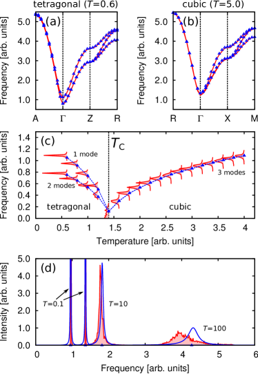
Figure 1: (Color online.) Dynamical properties of our model system. We show the results obtained from our approach based on MC simulations (blue) and the exact MD results (red). Panels (a) and (b): Phonon bands at two different $T$’s. Panel (c): Spectrum at the $\Gamma$ point, for $T$’s around the critical temperature $T_{\rm C}$. Panel (d): $\Gamma$ spectrum at selected $T$’s. All spectra are normalized to unity. See text for more details.

Figures 1(a) and 1(b) show the phonon bands at low and high $T$’s, respectively. The MD results were obtained from the first moment of the peaks in the spectrum given by the trace of $\widetilde{C}_{\mathbf{q},\alpha\beta}^{v^{\prime}v^{\prime}}(\omega)$. The MC results were obtained by diagonalizing $\mu_{\mathbf{q},\alpha\beta}^{v^{\prime},2}$ within our effective-harmonic approximation [Eq. (16)]. The agreement is excellent.

Figure 1(c) shows the $T$-dependent frequencies of the phonons at the $\Gamma$ point ($\mathbf{q}=0$). In the cubic phase, the frequencies decrease as $T$ is reduced, and essentially vanish at the critical temperature $T_{\rm C}$. Then, below $T_{\rm C}$ the frequencies increase as $T$ decreases. We have three $\Gamma$ phonons in both phases: they are three-fold degenerate in the cubic structure, but split in two groups when the symmetry is lowered to tetragonal. In the figure we show the trace of the $\widetilde{C}_{\Gamma,\alpha\beta}^{\bar{x}^{\prime}\bar{x}^{\prime}}(\omega)$ functions resulting from MD simulations, as well as the frequencies computed at the effective-harmonic level by diagonalizing $\mu_{\Gamma,\alpha\beta}^{\bar{x}^{\prime},0}$ obtained from MC. This approximation gives excellent results, even in the immediate vicinity of $T_{\rm C}$ where the system is strongly anharmonic.

Figure 1(d) shows the line shapes from the continued-fraction representation of $C_{\Gamma,aa}^{\bar{x}^{\prime}\bar{x}^{\prime}}(\omega)$, using up to the sixth-order moments, together with the MD results. We can appreciate that the widths of the peaks obtained with our method are semi-quantiatively correct. We include a result at an unrealistically high $T=100$, where the peak broadening is very significant. Even in such extreme conditions, our approximate spectral function provides a fair representation of the exact one.

Final remarks.– We have shown that the main features of classical vibrational spectra can be accurately computed from knowledge of the low-order moments of the appropriate time-correlation functions. More precisely, we have presented a way to compute a normal-mode-like basis that renders the low-order moments diagonal, which allows us to approximate the full spectrium by a collection of anharmonic oscillators [Eq. (15)]. Further, we have introduced an effective-harmonic approximation [Eq. (16)] that makes it possible to obtain very accurate results for the vibrational frequencies from simple statistical averages of atomic positions or forces. We have also shown that it is possible to reproduce the line shape of the spectral functions in a semi-quantitative way, provided higher moments are available.

The moments can be obtained as thermal averages from MC simulations. Alternatively, one may obtain them from MD simulations, without the need to explicitly compute the time-correlation functions; this should allow for shorter MD runs (only as long as needed to compute accurate thermal averages) and simplify the use of thermostats (as their interfering with the dynamics would be unimportant).

Our effective-harmonic treatment provides a rigorous justification for some of the assumptions underlying previous schemes in the literature hellman11 ; brooks95 ; wheeler03 . Further, first-principles methods like the one proposed in Ref. hellman11, could greatly benefit from results such as the identity $\langle\partial^{2}V/\partial x_{i}\partial x_{j}\rangle$ = $\beta\langle(\partial V/\partial x_{i})(\partial V/\partial x_{j})\rangle$, which we have proven here and constitutes a conveneint way to obtain the thermal-averaged force-constant matrix (computationally very costly) from appropriate products of forces (readily available). Finally, our effective-harmonic approximation can be connected with quasi-harmonic methods that have been applied in a variety of contexts book-dove05 ; goodwin04 ; goodwin05 ; our results support the applicability of such schemes even in cases with significant anharmonicity.

We hope the methods here discussed will become standard tools in classical simulations, where they can be used to a great advantage.

Work supported by the EC-FP7 project OxIDes (Grant No. CP-FP 228989-2) and MINECO-Spain (Grants No. MAT2010-18113, No. MAT2010-10093-E, and No. CSD2007-00041). Discussions with J.C. Wojdeł are gratefully acknowledged.

References

- (1) O. Hellman, I. A. Abrikosov, and S. I. Simak, Phys. Rev. B 84, 180301 (2011)
- (2) B. R. Brooks, D. Janežič, and M. Karplus, Journal of Computational Chemistry 16, 1522 (1995)
- (3) R. A. Wheeler, H. Dong, and S. E. Boesch, ChemPhysChem 4, 382 (2003)
- (4) M. T. Dove, Introduction to Lattice Dynamics, Cambridge Topics in Mineral Physics and Chemistry (Cambridge University Press, 2005) ISBN 9780521398947
- (5) A. L. Goodwin, M. G. Tucker, M. T. Dove, and D. A. Keen, Physical Review Letters 93, 075502 (2004)
- (6) A. L. Goodwin, M. G. Tucker, E. R. Cope, M. T. Dove, and D. A. Keen, Physical Review B 72, 214304 (2005)
- (7) J. H. Van Vleck, Physical Review 74, 1168 (1948)
- (8) P. G. De Gennes, Physica 25, 825 (1959)
- (9) H. Mori, Progress of Theoretical Physics 34, 399 (1965)
- (10) U. M. Balucani, H. Lee, and V. Tognetti, Physics Reports 373, 409 (2003)
- (11) A. Cuccoli, V. Tognetti, A. A. Maradudin, A. R. McGurn, and R. Vaia, Phys. Rev. B 46, 8839 (1992)
- (12) A. Cuccoli, V. Tognetti, A. A. Maradudin, A. R. McGurn, and R. Vaia, Phys. Rev. B 48, 7015 (1993)
- (13) E. R. Cowley and F. Zekaria, Phys. Rev. B 50, 16380 (1994)
- (14) A. Macchi, A. A. Maradudin, and V. Tognetti, Phys. Rev. B 53, 5363 (1996)
- (15) The intermediate scattering function for neutron diffraction can be approximated as , where the sum runs over the cell vectors and , the atoms and , and the spatial directions and . is hermitian, and real; thus, only the real part of the off-diagonal elements contributes to the sum. Additionally, the vibrational density of states is often computed as , which is real; here again, the imaginary part of the off-diagonal spectral functions plays no role.
- (16) We can write the autocorrelation functions and without a tilde because they are even, as the corresponding spectral functions and are real.
- (17) The statistical methods we used are standard. A description can be found, for example, in Ref. allen89, .
- (18) M. P. Allen and D. J. Tildesley, Computer Simulation of Liquids, Oxford science publications (Oxford University Press, USA, 1989) ISBN 0198556454
- (19) A. N. Rubtsov, J. Hlinka, and T. Janssen, Physical Review E 61, 126 (2000)
- (20) This kind of models have been studied extensively (see Ref. bruce80, for a review) and solved in approximate ways. Our method might seem related with some of the mean-field schemes discussed in the literature, such as the so-called independent-mode approximation. However, that resemblance is misleading, as we do simulate the true equilibrium state of the material, and introduce approximations only to extract the dynamical information.
- (21) A. D. Bruce, Advances in Physics 29, 111 (1980)
- (22) The so-called displacive and order-disorder (OD) limits for a phase transition can be studied with the model rubtsov00 . In the OD limit, the soft-mode vibrational spectrum presents additional features that do not correspond to those of a regular phonon. Our scheme is not well suited to render accurate results in such a case.