Abstract

We start a systematic investigation of the possibility to have supersymmetry (SUSY) to be an asymptotic state of the gauge theory in the high energy (UV) limit, due to the renormalization group running of coupling constants of the theory. The answer on whether this situation takes place or not, can be resolved by dealing with the running of the ratios between Yukawa and scalar couplings to the gauge coupling. The behavior of these ratios does not depend too much on whether gauge coupling is asymptotically free (AF) or not. It can be shown that the UV stable fixed point for the Yukawa coupling is not supersymmetric. Taking this into account, one can break down SUSY only in the scalar coupling sector. We consider two simplest examples of such breaking, namely $N=1$ supersymmetric QED and QCD. In one of the cases one can construct an example of SUSY being restored in the UV regime.

Keywords:   Renormalization group,  Supersymmetry,  Asymptotic properties.

PACS:  11.10.Hi,  11.15.-q,  11.10.Jj.  

MSC-AMS:  81T60,   81T17,   81T15.  

1 Introduction

One of the strongest theoretical motivations for SUSY is its ability to soften the high-energy behavior of quantum field theories by reducing the number of uncorrelated ultraviolet divergences. This is because in supersymmetric theories there are some restrictions on both the number of the fermionic and bosonic degrees of freedom of the theory and on the values of the coupling constants. These restrictions provide cancellations between fermionic and bosonic contributions to the ultraviolet divergences, thus providing a best high-energy behavior. Specifically, supersymmetry ensures the absence of quadratic divergences to all orders in the loop expansion. This exciting feature of supersymmetry offers a hope of solving the hierarchy problem [1, 2]. Roughly speaking, the solution to this problem consists in explaining the reason for the enormous ratio between the Planck energy scale, $\approx 10^{19}$ GeV, and the energy scale $\approx 300$ GeV that characterizes the Standard Model of the particle physics.

Even if the power-like divergences cancel, one has to deal with the logarithmic divergences. In principle, SUSY enables one to consider examples of a field theory with vanishing beta-functions, see, e.g., [3, 4, 5, 6, 7, 8]. The most of these examples are based on the theories with extended supersymmetry .

Renormalizable quantum field theories without supersymmetry like the Minimal Standard Model of the particle physics (MSM) suffer from the quadratic divergence problem, although they are very successful from the phenomenological point of view. In this type of theory, a systematic treatment of divergent integrals in perturbation theory was development by means of suitable renormalization schemes. Compared to this, the gauge models with SUSY are not currently enjoying much support from the phenomenological side, despite there are still good chances to see SUSY at the LHC (see, e.g., [10]).

The world of unbroken SUSY could be perfect, but it is not a real thing. One of the difficulties of phenomenological SUSY is that it should be broken at low energies, at the first place this is needed to reproduce MSM. There are different approaches to break SUSY, e.g., dynamical [11] and soft [12] breaking schemes. In both these cases the realistic SUSY imposes some strong constrains on the parameters of the theory, such as masses and couplings [13]. It is tentative to formulate and study the following question: is it possible to reduce these constrains such that the main advantage of SUSY, namely the natural solution of hierarchy problem, remains valid? One of the possibilities has been suggested long ago by Odintsov and Shapiro [14] (see also [15]), on the basis of renormalization group running of the parameters. In this work it was proposed to consider a rigid breaking of SUSY in the theory with zero beta-functions and look for the situation when both SUSY and finiteness get restored in the UV by quantum effects and corresponding running of the couplings. It looks interesting to generalize this result for the realistic versions of supersymmetric Stardard Model or Grand Unification Theories and see what would be the possible impact of the breaking of SUSY in the couplings sector to the SUSY breaking mechanisms.

In the present work, we study the possibility that if the restrictions on the coupling constants imposed by supersymmetry are violated at low energies, then they can be restored in the UV regime. To do so, we mainly use the renormalization group method to study the behavior of the scalar coupling constants, because the situation with Yukawa couplings is much more simple. The result depends on the details of scalar self-interaction and in the present work we intend to deal with the simplest possible models, such that the situation becomes qualitatively clear. For this reason we consider an Abelian and non-Abelian cases with the simplest possible fields content admitting SUSY.

This paper is organized as follows. In Sect. 2 we present a brief discussion of the running of Yukawa coupling and also formulate the framework for dealing with scalar couplings. In Sect. 3 we explore the behavior of the scalar coupling constants within supersymmetric QED, assuming that these constants initially differ from their values imposed by supersymmetry. According to what was explained above, in this section we simply ignore the fact that supersymmetric QED is not AF theory. It is shown that there is an example of asymptotic SUSY in this case, however the theory with soft SUSY breaking meets certain physical difficulties in this case. In Sect. 4 we analyze the same possibility in a supersymmetric QCD and show that the situation is different in this case. Finally, a summary and discussion of the results is given in Sect. 5.

2 Model-indepent part: Yukawa couplings running

Let us start by describing the way SUSY can be broken and restored in the UV limit [14, 16]. SUSY implies rigid relations between gauge $g$, Yukawa $h$ and scalar $f$ couplings. For the sake of simplicity, consider a theory with a single Yukawa coupling and assume that the SUSY relation between the Yukawa and gauge couplings has the form $h=g$. Let us now break this relation down and assume that the value of ${\bar{h}}=h/g$ is arbitrary. It is well known (see, e.g., [17]), that the general form of the renormalization group equation (all consideration will be restricted to one-loop order) for $h$ has the form

$$\frac{dh^{2}}{dt}=\mu\,\frac{dh^{2}}{d\mu}=a_{1}h^{4}-a_{2}g^{2}h^{2}\,,\qquad h(\mu_{0})=h_{0}\,,$$ (1)

where we introduced a useful notation $t=\log(\mu/\mu_{0})$ and $a_{1,2}$ are positive and otherwise model-dependent coefficients. Taking into account the renormalization group equation for $g(t)$,

$$\frac{dg^{2}}{dt}=\pm b^{2}g^{4}\,,$$ (2)

we can write the equation for the ratio in the form

$$\frac{d{\bar{h}}^{2}}{dt}=g^{2}(t)\big{[}a_{1}{\bar{h}}^{4}-(a_{2}\pm b^{2}){\bar{h}}^{2}\big{]}\,.$$ (3)

It is easy to see that the existence of SUSY imposes a constraint on the values of the coefficients of the last equation. One can see that the last equation indicates a universal fixed point ${\bar{h}}=0$. Furthermore, we know that the value of ${\bar{h}}=1$ corresponding to SUSY is also a fixed point, because the theory with SUSY is renormalizable [18, 19]. Therefore, the Eq.(3) can be rewritten as

$$\frac{d{\bar{h}}^{2}}{dt}=a_{1}g^{2}(t)\,{\bar{h}}^{2}\,\big{[}{\bar{h}}^{2}-1\big{]}\,.$$ (4)

In the case of finite $g\equiv g_{0}$ or asymptotically free theory, this means that, independent on the value of $a_{1}$ the SUSY fixed point is unstable in the UV limit. Any violation of the constraint $h=g$ such that $h_{0}<g_{0}$ means that the renormalization group trajectory for ${\bar{h}}(t)$ end at the zero value in the UV fixed point. In case $h_{0}>g_{0}$ one can observe the behavior ${\bar{h}}(t)\to\infty$ in the UV, when $\,t\to\infty$, such that the SUSY is not restored in the UV anyway. The conclusion we can draw is that the violation of the SUSY constraint for the Yukawa coupling does not lead to the UV restoration of SUSY. Hence in what follows we shall always assume that the ratio $h/g=1$ is not violated and concentrate our attention on the sector of scalar coupling $f$, where we still have a chance to meet asymptotic SUSY.

3 Abelian Case

First, we consider the supersymmetric QED. The field content consist of a Dirac field $\psi$, two complex scalar fields $\phi_{+}$ and $\phi_{-}$, a vector field $A_{\mu}$ and four-component Majorana field $\lambda_{M}$. The Lagrange density has the form

$$\mathcal{L}_{\textrm{SQED}} = -\frac{1}{4}F_{\mu\nu}F^{\mu\nu}+\frac{i}{2}\bar{\lambda}_{M}\gamma^{\mu}\partial_{\mu}\lambda_{M}+i\bar{\psi}\gamma^{\mu}D_{\mu}\psi+\left|D_{\mu}\phi_{+}\right|^{2}+\left|D_{\mu}^{\dagger}\phi_{-}\right|^{2}$$ (5)

$$-\sqrt{2}g\left(\phi_{+}^{*}\bar{\lambda}_{M}\psi_{L}+\bar{\psi_{L}}\lambda_{M}\phi_{+}-\phi_{-}\bar{\lambda}_{M}\psi_{R}-\bar{\psi_{R}}\lambda_{M}\phi_{-}^{*}\right)$$

$$-\frac{g^{2}}{2}\left(\left|\phi_{+}\right|^{2}-\left|\phi_{-}\right|^{2}\right)^{2}\,+\,\textrm{(mass terms)}\,+\,\textrm{(gauge-fixing terms)}\,,$$

where $\psi_{L,\,R}\equiv\frac{1}{2}\left(1\mp\gamma_{5}\right)\psi$ and $D_{\mu}=\partial_{\mu}+igA_{\mu}$. The mass terms are not relevant to the present analysis, and the gauge-fixing terms here are assumed to correspond the Landau gauge. It is important that supersymmetry imposes a relation on the Yukawa and scalar $\left|\phi_{\pm}\right|^{4}$ couplings, i.e., both these couplings are proportional to the gauge coupling $g$.

Now we consider the possibility that if we break these relations between coupling constants imposed by supersymmetry in Eq.(5), they will be recovered at high energies. In other words, will they appear asymptotically with supersymmetry restored or not?

In order to study this possibility, we trade the term

$$-\frac{g^{2}}{2}\left(\left|\phi_{+}\right|^{2}-\left|\phi_{-}\right|^{2}\right)^{2}$$

in Eq.(5) for a more general expression

$$-\frac{f_{+}}{4}\left|\phi_{+}\right|^{4}-\frac{f_{-}}{4}\left|\phi_{-}\right|^{4}+f_{\pm}\left|\phi_{+}\right|^{2}\left|\phi_{-}\right|^{2}\,.$$ (6)

After this modification the theory remains renormalizable, but it is not supersymmetric anymore. In what follows we shall consider the one-loop approximation to the renormalization group equations for the effective couplings $f_{+}(t)$, $f_{-}(t)$ and $f_{\pm}(t)$ and analyze the asymptotic behavior of these effective coupling constants. In order to perform this consideration, we divide our analysis into three cases:

• Case 1: $f_{+}=f_{-}=2f_{\pm}=f$ with $f\neq 2g^{2}$;

• Case 2: $f_{+}=f$, $f_{-}=2g^{2}$ and $f_{\pm}=g^{2}$ (or equivalently $f_{-}=f$, $f_{+}=2g^{2}$ and $f_{\pm}=g^{2}$) with $f\neq 2g^{2}$;

• Case 3: $f_{+}=f_{-}=2g^{2}$ and $f_{\pm}=f$ with $f\neq g^{2}$.

Note that, in all of the cases above, the only symmetry of the Lagrangian in Eq.(5) that has been broken is supersymmetry. The gauge symmetry and the discrete symmetry usually called $R-$parity are still held in the three cases.

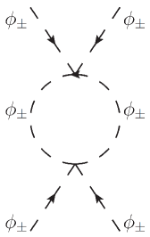
(a) ref1

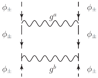
(b) ref2

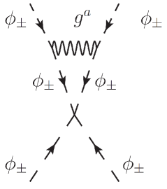
(c) ref3

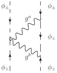
(d) ref4

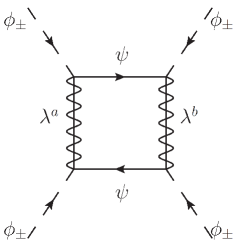
(e) ref5

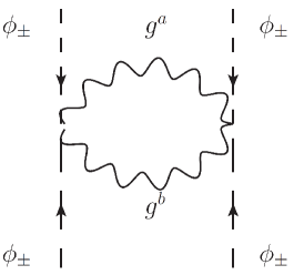
(f) ref6

?figurename? 1: One-loop diagrams contributing to the $\beta$-functions for scalar self-couplings, discussed in the next two Sections.

The diagrams needed to calculate the one-loop $\beta$-functions in the theory with broken SUSY are presented in Fig.1. We will not discuss the details of this calculations, which are quite standard (see, e.g., [17, 20]), but go directly to the renormalization group equations of our interest. In the Case 1, we can write down the scalar $\beta$-function in the following form

$$\beta_{f} = \frac{1}{{(4\pi)^{2}}}\left(6f^{2}-4fg^{2}-8g^{4}\right)\,.$$ (7)

In order to analyze the asymptotic behavior of $f(t)$, it is convenient to define $\bar{f}\equiv f/g^{2}$. Then we arrive at the renormalization group equation

$$\frac{d\bar{f}}{dt}\,=\,\beta_{\bar{f}} = \frac{6\,g^{2}}{(4\pi)^{2}}\,\Big{(}\bar{f}-2\Big{)}\Big{(}\bar{f}+\frac{2}{3}\Big{)}\,,$$ (8)

where we have used the known expression $\beta_{g}=2g^{3}/(4\pi)^{2}$. From Eq.(8), we see that the $\beta_{\bar{f}}$ function has one fixed point that correspond to the supersymmetric case ($\bar{f}_{\textrm{SUSY}}=2$), as it should be, since the supersymmetry is not anomalous at one-loop. At the same time, one can see that the supersymmetric fixed point is stable in the infrared, i.e. the relation $f/g^{2}=2$ imposed by supersymmetry at tree level is restored when $t\rightarrow-\infty$. Concerning the UV limit it is easy to see that there in no asymptotic SUSY in the Case 1.

Now, let us continue with the Case 2. In this case the $\beta_{f}$ and $\beta_{\bar{f}}$ take the form

$$\beta_{f} = \frac{1}{(4\pi)^{2}}\left(5f^{2}-4fg^{2}-4g^{4}\right),$$

and

$$\frac{d\bar{f}}{dt}\,=\,\beta_{\bar{f}} = \frac{g^{2}}{(4\pi)^{2}}\,5\,\left(\bar{f}-2\right)\left(\bar{f}+\frac{2}{5}\right)\,.$$ (9)

From Eq.(9), we see that in this case the supersymmetric value, $\bar{f}_{\textrm{SUSY}}=2$ is, once again, an infrared stable fixed point. Consequently, there is no asymptotic SUSY in the UV limit in this case.

Finally, we find that in Case 3, the $\beta_{f}$ and $\beta_{\bar{f}}$ functions can be written as

$$\beta_{f} = -\frac{1}{(4\pi)^{2}}\left(f^{2}-fg^{2}-g^{4}\right),$$

and

$$\frac{d\bar{f}}{dt}\,=\,\beta_{\bar{f}} = -\frac{g^{2}}{(4\pi)^{2}}\left(\bar{f}-1\right)\left(\bar{f}+1\right)\,.$$ (10)

From Eq.(10) one can see that, this time, the supersymmetric value $\bar{f}_{\textrm{SUSY}}=1$, is an ultraviolet stable fixed point. In other words, it is an attractive fixed point for the initial values of the renormalization group trajectory with the initial point satisfying the inequality $\bar{f}_{0}>-1$. In this case $\bar{f}\rightarrow\bar{f}_{\textrm{SUSY}}$ when $t$ goes to $\infty$.

4 Non-Abelian Case

As a second example, consider a supersymmetric Non-Abelian theory. For our purposes, it is enough to take the case of such a theory with one “flavor” of “quarks” and “squarks”, taking the gauge group to be $SU\left(N\right)$, with $(N\geq 2)$. Here, we are using the terms flavor, quarks and squarks, despite the theory is reduced compared to a real QCD. Also, what we mean by one flavor is that there is both a left-handed quark (and a superpartner squark) in the $N-$dimensional (fundamental) representation of the $SU(N)$ gauge group as well as a left-handed quark in the anti-fundamental representation. Indeed, this theory is often referred to in the literature as supersymmetric QCD. The Lagrange density has the form

$${\cal L}_{\textrm{SQCD}} = -\frac{1}{4}F_{\mu\nu}^{a}F^{\mu\nu a}+\frac{i}{2}\bar{\lambda}_{M}^{a}\gamma^{\mu}\left(\delta^{ac}\partial_{\mu}-gt^{abc}A_{\mu}^{b}\right)\lambda_{M}^{c}+i\bar{\psi}\gamma^{\mu}D_{\mu}\psi+\left|D_{\mu}\phi_{+}\right|^{2}+\left|D_{\mu}\phi_{-}^{*}\right|^{2}$$ (11)

$$-\sqrt{2}g\left(\phi_{+}^{\dagger}\bar{\lambda}_{M}^{a}T^{a}\psi_{L}+\bar{\psi}_{L}T^{a}\lambda_{M}^{a}\phi_{+}-\phi_{-}^{T}\bar{\lambda}_{M}^{a}T^{a}\psi_{R}-\bar{\psi_{R}}\lambda_{M}^{a}T^{a}\phi_{-}^{*}\right)$$

$$-\frac{1}{2}g^{2}\sum_{a=1}^{N^{2}-1}\left(\phi_{+}^{\dagger}T^{a}\phi_{+}-\phi_{-}^{\dagger}\bar{T}^{a}\phi_{-}\right)^{2}+\,(\textrm{mass terms)}$$

$$+\,\textrm{(gauge-fixing and ghost terms)}\,,$$

where $D_{\mu}=\partial_{\mu}+igT^{a}A_{\mu}^{a}$, with $T^{a}$, $a=1,\cdots,\,N^{2}-1$, being the generators of the $SU\left(N\right)$ group in the fundamental representation and $\bar{T}^{a}$ are the corresponding complex conjugate matrix; $t^{abc}$ are the structure constants for $SU\left(N\right)$ in the standard form; the hermitian conjugation and the transposition in Eq.(11) are in the $SU\left(N\right)$ internal space.

Now, we proceed by analogy with the Abelian case and trade the scalar self-interaction term

$$-\frac{1}{2}g^{2}\sum_{a=1}^{N^{2}-1}\left(\phi_{+}^{\dagger}T^{a}\phi_{+}-\phi_{-}^{\dagger}\bar{T}^{a}\phi_{-}\right)^{2}$$

in Eq.(11) by

$$-\frac{1}{4}\,f_{+}\left(\frac{N-1}{N}\right)\left(\phi_{+}^{\dagger}\phi_{+}\right)^{2}-\frac{1}{4}\,f_{-}\left(\frac{N-1}{N}\right)\left(\phi_{-}^{\dagger}\phi_{-}\right)^{2}\,,$$

$$+\frac{1}{2}\,f_{1}\left(\phi_{+}^{\dagger}\phi_{-}^{*}\right)\left(\phi_{-}^{*\dagger}\phi_{+}\right)-\frac{1}{2N}\,f_{2}\left(\phi_{+}^{\dagger}\phi_{+}\right)\left(\phi_{-}^{\dagger}\phi_{-}\right),$$ (12)

where we have used the relation

$$\sum\limits_{a=1}^{N^{2}-1}T_{ML}^{a}T_{NP}^{a}=\frac{1}{2}\left(\delta_{MP}\delta_{LN}-\frac{1}{N}\delta_{ML}\delta_{NP}\right)\,,$$

where $M,\,P,\,L,\,N$ are the indices in the internal gauge space. Now, for the sake of simplicity, we divide our analysis into three cases:

• Case 1: $f_{+}=f_{-}=f_{1}=f_{2}=f$ with $f\neq g^{2}$;

• Case 2: $f_{+}=f,$ $f_{-}=f_{1}=f_{2}=g^{2}$ (or equivalently $f_{-}=f$, $f_{+}=f_{1}=f_{2}=g^{2}$) with $f\neq g^{2}$;

• Case 3: $f_{+}=f_{-}=g^{2}$, $f_{1}\neq g^{2}$ and $f_{2}\neq g^{2}$.

In Case 1, we can write down the $\beta_{f}$ and $\beta_{\bar{f}}$ functions in the one-loop approximation as

$$\beta_{f} = \frac{1}{(4\pi)^{2}}\,\left[\frac{N^{2}+4N-4}{N}f^{2}-2\frac{N^{2}-1}{N}fg^{2}-\frac{5N^{2}+2N-2}{N}g^{4}\right],$$

and

$$\frac{d\bar{f}}{dt}\,=\,\beta_{\bar{f}} = \frac{g^{2}}{(4\pi)^{2}}\,\frac{N^{2}+4N-4}{N}\,\left(\bar{f}-1\right)\left(\bar{f}+\frac{5N^{2}+2N-2}{N^{2}+4N-4}\right),$$ (13)

where $\bar{f}\equiv f/g^{2}$ and we also have used $\beta_{g}=-g^{3}\left(3N-1\right)/(4\pi)^{2}$.

For $N\geq 2$, we have

$$\frac{N^{2}+4N-4}{N}>0\quad\mbox{and}\quad\frac{5N^{2}+2N-2}{N^{2}+4N-4}>0\,.$$

Then, $\bar{f}_{\textrm{SUSY}}=1$ is an infrared-stable fixed point.

In Case 2, the $\beta_{f}$ and $\beta_{\bar{f}}$ functions in the one-loop approximation have the following form

$$\beta_{f} = \frac{1}{(4\pi)^{2}}\,\left[\frac{\left(N-1\right)\left(N+4\right)}{N}f^{2}-2\frac{N^{2}-1}{N}fg^{2}-\frac{5N^{2}+N-2}{N}g^{4}\right],$$

and

$$\frac{d\bar{f}}{dt}\,=\,\beta_{\bar{f}} = \frac{1}{(4\pi)^{2}}\,\frac{\left(N-1\right)\left(N+4\right)}{N}\,\left(\bar{f}-1\right)\left(\bar{f}+\frac{5N^{2}+N-2}{\left(N-1\right)\left(N+4\right)}\right)\,.$$ (14)

For $N\geq 2$, we have

$$\frac{\left(N-1\right)\left(N+4\right)}{N}>0\quad\mbox{and}\quad\frac{5N^{2}+N-2}{\left(N-1\right)\left(N+4\right)}>0\,.$$

Hence, once again, $\bar{f}_{\textrm{SUSY}}=1$ is an infrared-stable fixed point.

Finally, in the Case 3 we consider simultaneously $f_{1}\neq g^{2}$ and $f_{2}\neq g^{2}$. At the one-loop approximation the $\beta_{f_{1}}$, $\beta_{f_{2}}$, $\beta_{\bar{f}_{1}}$ and $\beta_{\bar{f}_{2}}$ functions can be written as

$$\beta_{f_{1}} = \frac{1}{(4\pi)^{2}}\,\left[-Nf_{1}^{2}+\frac{4}{N}f_{1}f_{2}+2\left(1-N\right)f_{1}g^{2}-\left(3N+\frac{4}{N}\right)g^{4}\right],$$ (15)

$$\beta_{f_{2}} = \frac{1}{(4\pi)^{2}}\,\left[\frac{2}{N}f_{2}^{2}+Nf_{1}^{2}+2\left(1-N\right)f_{1}g^{2}-\left(5N+\frac{2}{N}\right)g^{4}\right],$$ (16)

and

$$\beta_{\bar{f}_{1}} = \frac{g^{2}}{(4\pi)^{2}}\,\left[-N\left(\bar{f}_{1}-1\right)\left(\bar{f}_{1}-3\right)+\frac{4}{N}\left(\bar{f}_{1}\bar{f}_{2}-1\right)\right],$$ (17)

$$\beta_{\bar{f}_{2}} = \frac{g^{2}}{(4\pi)^{2}}\,\left[\frac{2}{N}\left(\bar{f}_{2}-1\right)\left(\bar{f}_{2}+3N^{2}+1\right)+N\left(\bar{f}_{1}-1\right)^{2}+2\left(\bar{f}_{1}-\bar{f}_{2}\right)\right],$$ (18)

where $\bar{f}_{1}\equiv f_{1}/g^{2}$ and $\bar{f}_{2}\equiv f_{2}/g^{2}$. Using Eqs. (17) and (18), we can analyze the perturbative behavior of $\beta_{\bar{f}_{1}}$ and $\beta_{\bar{f}_{2}}$ in the neighborhood of the supersymmetric fixed points, $\bar{f}_{1\,\textrm{SUSY}}=1$ and $\bar{f}_{2\,\textrm{SUSY}}=1$.

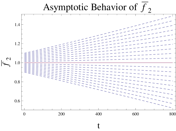
?figurename? 2: Behavior of $\bar{f}_{2}$ vs $t$ for supersymmetric $SU\left(3\right)$. We have used $t_{0}=0.2$, $\bar{f}_{1}\left(t_{0}\right)=1$ and $\bar{f}_{2}\left(t_{0}\right)=0.9+k\cdot\Delta$ (with $\Delta=0.01$, and $k=0,\cdots,20$) as initial conditions. The dashed lines correspond to $\bar{f}_{2}(t)$ for the different values of $\bar{f}_{2}\left(t_{0}\right)$. We see from the figure that $\bar{f}_{2\,\textrm{SUSY}}=1$ is an ultraviolet unstable fixed point.

First, we consider the case that $\bar{f}_{1}=\bar{f}_{1\,\textrm{SUSY}}=1$, but $\bar{f}_{2}\neq\bar{f}_{2\,\textrm{SUSY}}$. Note that, despite the fact that $\bar{f}_{2}$ is not actually equal to $\bar{f}_{2\,\textrm{SUSY}}$, we consider it to be close. Doing so, we have

$$\left.\beta_{\bar{f}_{2}}\right|_{\bar{f}_{1}=\bar{f}_{1\textrm{SUSY}}} = \frac{g^{2}}{(4\pi)^{2}}\,\frac{2}{N}\left(\bar{f}_{2}-1\right)\left(\bar{f}_{2}+3N^{2}-N+1\right).$$ (19)

From Eq.(19) above, we see that $\bar{f}_{2\,\textrm{SUSY}}$ is an infrared stable fixed point. The same analysis can be done for the case that $\bar{f}_{2}=\bar{f}_{2\,\textrm{SUSY}}$, but $\bar{f}_{1}\neq\bar{f}_{1\,\textrm{SUSY}}$ . In this case, we have

$$\left.\beta_{\bar{f}_{1}}\right|_{\bar{f}_{2}=\bar{f}_{2\textrm{SUSY}}} = -\frac{g^{2}}{(4\pi)^{2}}\,N\left(\bar{f}_{1}-1\right)\Big{[}\bar{f}_{1}-\Big{(}3+\frac{4}{N^{2}}\Big{)}\Big{]}\,.$$ (20)

As in the previous case, from Eq.(20), one can see that $\bar{f}_{1\,\textrm{SUSY}}$ is an infrared stable fixed point. In order to illustrate the behavior of $\bar{f}_{2}$ in function of $t$, we have numerically integrated the Eqs.(17) and (18) for the particular case of supersymmetric $SU\left(3\right)$. We have used the initial conditions  $g\left(t_{0}\right)=0.2$,  $\bar{f}_{1}\left(t_{0}\right)=1$ and $\bar{f}_{2}\left(t_{0}\right)=0.9+k\cdot\Delta$, where $\Delta=0.01$ and $k=0,\cdots,20$. The plots illustrating the running of $\bar{f}_{2}$ are shown in the Fig.2.

5 Conclusions

The theories with supersymmetric particle/field content, but with a non-supersymmetric choice of coupling constants are potentially interesting, especially because SUSY may get restored asymptotically, in the UV limit [14]. If this asymptotic behavior really takes place, one may hope to solve the hierarchy problem with less restrictions on the parameters of the theory, which maybe a welcome feature from the phenomenological viewpoint. In order to address this possibility, we have considered a one-loop running in the models with violated SUSY. The fate of the violation in the Yukawa sector can be traced back in the general form, and we conclude that the SUSY is always an IR fixed point, independent on the details of the theory. Then our main attention has been paid to the situation with a violation in the sector of scalar self-interaction couplings.

To summarize our results, we have shown that in both Abelian and non-Abelian cases, the function $\beta_{\bar{f}}$, at one-loop approximation, has the following form:

$$\beta_{\bar{f}} = c_{1}\,\left(\bar{f}-\bar{f}_{\textrm{SUSY}}\right)\left(\bar{f}-\bar{f}_{1}\right)\,,$$ (21)

where $c_{1}$ is the model-dependent coefficient and the value of $\bar{f}_{1}$ corresponds to a non-supersymmetric version of the gauge theory.

We have considered several particular ways to violate SUSY in both Abelian and non-Abelian models. In most cases we have found that the two fixed point satisfy the inequality $\bar{f}_{\textrm{SUSY}}>\bar{f}_{1}$. For $c_{1}>0$ this means that the SUSY is an IR-stable fixed point, and not an UV-stable. Obviously, the IR running based on the Minimal Subtraction renormalization scheme is not a clear issue, because the sparticle are supposed to be massive and, therefore, the running (if any) should be strongly modified by decoupling of massive degrees of freedom.

Only in one particular case, with Abelian gauge group, we have found the UV-stable asymptotic SUSY, due to the negative sign of the $c_{1}$ coefficient. Let us note that the negative sign here does not lead to problems with stability, because other $\beta$-functions remain positive. The real advantage of dealing with Abelian model is its simplicity, which gives an opportunity to better control the fixed points for the ratio between scalar and gauge couplings. The fact that the theory under consideration is Abelian does not look too important for the distribution of zeroes of $\beta_{\bar{f}}$, so we have simply ignored the positive sign of the $\beta$-function for the gauge coupling. Of course, it would be interesting to extend the present consideration to the more realistic cases of the gauge models with possible asymptotic SUSY.

In a similar situation (Case 3) in the supersymmetric QCD we have found $c_{1}<0$, but unfortunately with $\bar{f}_{\textrm{SUSY}}<\bar{f}_{1}$. As a consequence, $\bar{f}_{\textrm{SUSY}}$ is not an UV stable fixed point in this case. The particular examples considered here are not sufficient to see whether the consistent solution with UV asymptotic SUSY is possible or not, but is worthwhile to study this subject further.

All in all, it remains unclear whether the asymptotic SUSY can be achieved within some version of realistic supersymmetric gauge theory, including non-minimal Standard Model. Our consideration shows that this possibility can not be ruled out and therefore some further work in this direction looks interesting to do. In case of a positive output, the corresponding gauge theory would be a promising model to study particle phenomenology.