Dynamic Compression of in situ Grown Living Polymer Brush: Simulation and Experiment

Abstract

A comparative dynamic Monte Carlo simulation study of polydisperse living polymer brushes, created by surface initiated living polymerization, and conventional polymer monodisperse brush, comprising linear polymer chains, grafted to a planar substrate under good solvent conditions, is presented. The living brush is created by end-monomer (de)polymerization reaction after placing an array of initiators on a grafting plane in contact with a solution of initially non-bonded segments (monomers). At equilibrium, the monomer density profile $\phi(z)$ of the LPB is found to decline as $\phi(z)\propto z^{-\alpha}$ with the distance from the grafting plane $z$, while the distribution of chain lengths in the brush scales as $c(N)\propto N^{-\tau}$. The measured values $\alpha\approx 0.64$ and $\tau\approx 1.70$ are very close to those, predicted within the framework of the Diffusion-Limited Aggregation theory, $\alpha=2/3$ and $\tau=7/4$. At varying mean degree of polymerization (from $\langle L\rangle=28$ to $\langle L\rangle=170$) and effective grafting density (from $\sigma_{g}=0.0625$ to $\sigma_{g}=1.0$), we observe a nearly perfect agreement in the force-distance behavior of the simulated LPB with own experimental data obtained from colloidal probe AFM analysis on PNIPAAm brush and with data obtained by Plunkett et. al., [Langmuir 2006, 22, 4259] from SFA measurements on same polymer.

I Introduction

After the recent advances in the nanostructuring of surfaces, polymers can now be end-grafted on nanometer scale structures Dyer ; Gates . The recent progress in the production of nanoscale polymer structures has, however, only partially been matched by advances in the experimental methods of measuring the properties of such systems Kawaguchi . Available contactless methods, for example, optical methods, average the brush properties over areas that are larger than the nanoscale so that fine spatial resolution is lost. To retain sufficient spatial resolution, atomic force microscopy (AFM) is conventionally used Binnig ; Magonov ; Garcla ; Kaholek . However, the necessary contact between the AFM tip and the polymer thin layer distorts the layer and thus the object that it intends to study Wilder .

AFM measurements of polymers, tethered on surfaces with various geometries, illustrate a more general and fundamental class of problems, namely, the response of soft matter to external forces. Polymer brushes, that is, densely packed arrays of polymer chains end-attached to an interface, have been studied extensively (for reviews see Halperin1 ; Klein1 ; Szleifer ; Grest1 ; Kaholek ; Binder ) due to their ability to modify surface properties, prevent colloid aggregation, and enhance lubrication or adhesion Kaholek ; Napper ; Hamilton ; Pastorino . When properly designed, polymer brushes in good solvent conditions have been shown to remarkably reduce friction Klein2 . The brush structure and its properties can be controlled by tuning the grafting density, and variation of polymer molecular weight, temperature, and solvent quality Auroy1 . Numerous theoretical Alexander ; Milner1 ; Milner2 ; Halperin2 ; Biesheuvel1 ; Biesheuvel2 ; de Gennes ; Wijmans , experimental Auroy2 ; Cho ; Smith ; de Vos1 ; de Vos2 , and simulational Grest2 ; Murat1 ; Lai1 ; Lai2 ; Lai3 ; Neelov1 ; Neelov2 ; Neelov3 ; He ; Coluzza ; Seidel ; Kreer ; Dimitrov1 ; Dimitrov2 studies have examined the structure and properties of polymer brushes. There exist, however, sometimes significant differences between the theoretical and the experimental investigations of polymer brushes. So most theories assume strong stretching of polymer chains in the brush, while it is hard for an experimentalist to achieve densities high enough so as to meet this assumption Milner3 . The polydisperse nature of the synthesized brushes poses another significant difference. While it is practically impossible for an experimentalist to produce a perfectly monodisperse polymer brush, to the best of our knowledge, most of the theoretical works so far have not taken into consideration the intrinsic polydispersity of the brushes with a realistic chain length distribution, see, however, the early work of Milner et al. Milner4 .

The interaction between an AFM tip and a nanodesigned polymer brush bears resemblance to the problems mentioned above. Previous works on the interaction between a uniformly grafted polymer brush and an external object usually neglected effects of polydispersity and high grafting density of the tethered chains Jeon1 ; Jeon2 ; Subramanian ; McCoy ; Steels ; Pang even though the properties of living polymers in the bulk have been considered by Flory Flory , Wheeler Wheeler , Pfeuty Pfeuty and others. A step toward understanding the role of polydispersity in soft matter outdoor response was done by the investigation of “equilibrium polymers” (EP) as summarized in Wittmer2 . EPs (or, living polymers) denote polymer solutions where the chains are dynamic objects with the unique feature of constantly fluctuating lengths. Subject to external perturbation, concentration, or temperature change, they are able to respond via polymerization - depolymerization reactions allowing new thermodynamic and chemical equilibrium to be established. An important example of such constant process of dynamic equilibrium between polymers and their respective building units is that of surfactant molecules forming long flexible cylindrical aggregates, the so called wormlike giant micelles (GM) Wittmer2 , which break and recombine constantly at random points along the sequence. EPs are intrinsically polydisperse and their Molecular Weight distribution (MWD) in equilibrium is expected Cates1 ; Flory to follow an exponential decay with chain length.

An efficient way to create polymer brushes is the growth of living polymer chains from active sites on a surface whereby brushes with given polydispersity index and grafting density can be synthesized Vidal ; Ruehe . One of the earliest works investigating theoretically the growth of polymer chains from a surface was carried out by Wittmer et. al., Wittmer1 , combining elements of diffusion-limited aggregation (DLA) Witten with the theory of polydisperse strongly stretched polymer brushes Alexander ; Guiselin . Generalizing the “needle growth” problem Meakin , they considered the formation of the brush as a particular case of diffusion-limited aggregation without branching (DLAWB).

The interaction between a polydisperse grafted layer, commonly referred to as living polymer brush (LPB), and an AFM tip is similar to that of a polymer layer with a particle of mesoscopic size. A theoretical discussion of the latter has already been presented by Subramanian et. al., Subramanian . Their treatment considered both dense brush (high grafting density) and ’mushroom’ (low grafting density) regime. For fixed brushes, in which the anchoring points on the surface are immobile, they assumed that when the particle is pushed against the grafted chains, these chains undergo pure compression and do not splay. Under such an assumption, the force of compression (force $F$ divided by cross-sectional area of the compressing particle $A$) per unit area, $F/A$, does not depend on the radius of the compressing particle and is identical to the force for a brush pressed by a flat (infinite radius) plate. In the mushroom regime, they allowed the chains to deform and escape compression, and in this case Subramanian et. al., Subramanian found that the chains do splay to the side to avoid being compressed. A nanopatterned polydisperse polymer brush, however, is a much more complex system as its distributed correlation length is of the same order as the size of the system. Therefore, the brush can evade to the side, which is impossible for the monodisperse grafted brush, making the nanopatterned polydisperse brush effectively “softer”.

The force measured in an AFM experiment is rarely the quantity that one is ultimately interested in. The noteworthy exception to this statement are studies of the chemical nature of the brush surface where the degree of sticking is the sought-after information Magonov . In most other cases, the measured force $F$ first has to be converted, or “gauged”, to yield, for example, the brush density $\phi$. However, already for a homogeneously monodisperse polymer brush, computing the density $\phi$ is not possible from the knowledge of the force F alone - instead, additional information about the brush is needed Murat2 , such as its grafting density, $\sigma_{g}$, and this information frequently might not be available.

Still, for the case of monodisperse polymer brush, a relation between $F$ and $\phi$ always exists and it also does not depend on the transversal position of the AFM tip. All of this changes when a polydisperse polymer brush is considered instead. Even for the same brush, identical values of the force $F$ now correspond to different values of the density $\phi$ (or some other quantity of interest). This hinders a deeper understanding of the polymer brush properties via direct interpretation of AFM results.

Thus, the need to understand the response of polydisperse polymer brushes to local external forces is both fundamental and practical. In this communication, we first grow the polydisperse living polymer brush (LPB) in situ, monomer by monomer, from a functionalized seed carrying polymerization initiators, that is representative for a wider range of realistic systems. We then perform coarse grained off-lattice Monte-Carlo (MC) simulations Milchev4 ; Milchev6 of the interaction between the polydisperse living brush and a piston as representative for the AFM tip. The simulations represent roughly $2000-20000$ g/mol chains ($30-260$ coarse-grained monomers per chain) over a range of grafting densities. The high grafting densities examined in this study are achievable experimentally by “grafting from” techniques such as atom transfer radical polymerization (ATRP) von Werne ; Ell . Anticipating, we observe good agreement between simulational and experimental force - distance relationships.

The outline of the remainder of the paper is as follows. In the next Section II we sketch briefly the basis of the analytical treatment of LPB and the principal properties of living polymer brushes. In Section III we introduce the Monte Carlo model, employed in our study, and elucidate the salient features of the underlying algorithm.

The steric repulsion exerted on an impenetrable and semi-permeable wall in compression experiments with in situ grown LPB are presented in section V. In this section, we ask what happens when a layer of polydisperse polymer chains, grafted to a planar substrate by special groups, is subjected to external force (such a AFM tip). We also examine the effect of keeping the concentration of single non-grafted monomers in the box constant by using a semi-permeable wall so that the mean degree of polymerization in the brush does not change when the wall is moved. In the next section VI, the comparison between experiment and simulation is presented in more detail in view of our own experimental data obtained from colloidal probe AFM measurements. We briefly discuss the physical significance of the conversion factors for chain conformation sizes and length scales in real application, from the simulation to experiment. Eventually, in the last section, VII, we end this work by a brief summary of our findings.

II Theoretical Framework

II.1 Analytical Predictions of the Distribution of Chain Length

On a coarse-grained level, systems of living polymers are characterized by the monomer volume fraction $\phi$, the energy difference $E$ between saturated and unsaturated bond states, the persistence length $l_{p}$, and the excluded volume size $b$ of the monomer. For chains that are long compared to persistence length $l_{p}$, reversibility of the self-assembly process ensures that the molecular weight distribution (MWD) $c(N)$ of the polymeric species is in thermal equilibrium. Polymer brushes are usually created by means of surface-initiated polymerization Olivier and are characterized by non-negligible polydispersity Knoll . A large variety of synthetic routes for the generation of polymer brushes includes, e.g., ionic- Advincula , ring-opening- (ROP) Voccia , atom transfer radical- (ATRP) Jankova , and reversible addition-fragmentation chain transfer- (RAFT) Chiefari polymerization.

Most frequently in living polymers one observes a Flory-Schulz Molecular Weight Distribution (MWD) distribution of chain lengths:

$$c(N)=(1-p_{r})p_{r}^{N-1}=\frac{M_{0}}{M_{n}}\left(1-\frac{M_{0}}{M_{n}}\right)^{N-1},$$ (1)

where $c(N)$ is the fraction of chains with length $N$, $p_{r}\leq 1$ is the probability that a monomer has reacted, $M_{0}$ is the molecular weight of a monomer, and $M_{n}$ - the number-averaged molecular weight. Physically, Eq. (1) reflects a case when the reactivity of building units is independent of macromolecular weight.

In the case of dilute chains in the bulk, it has been shown that the MWD takes the form of Schulz-Zimm distribution Grosberg

$$c(l)=\frac{\gamma^{\gamma}}{\Gamma(\gamma)}\left(\frac{l}{\langle L\rangle}\right)^{\gamma-1}\exp\left(-\gamma\frac{l}{\langle L\rangle}\right)\quad$$ (2)

and an mean chain length is given by

$$\langle L\rangle\propto\phi^{\alpha}\exp(\delta E)\quad$$ (3)

In Eqs. (2) - (3 one has Wittmer2 $\alpha=\delta=(1+\gamma)^{-1}$ whereby $\gamma\approx 1.165$ in three dimensions.

In living polymers the semi-dilute conditions correspond to the case $L^{*}\ll\left<L\right>$ and $\phi>\phi^{*}$, where $L^{*}$ and $\phi^{*}$ mark the mean chain length and the density at crossover regime. Eventually, proceeding as in the ideal case, one may recover in the semi-dilute case a simple exponential expression for the molecular weight distribution,

$$c(l)=\frac{\phi}{\left<L\right>^{2}}{\rm exp}\left(-\frac{l}{\left<L\right>}\right),$$ (4)

with a slightly different expression for the average polymer length

$$\langle L\rangle\propto\phi^{\alpha}\exp(\delta E),\quad\delta=\frac{1}{2},\quad$$ (5)

where $\alpha=\frac{1}{2}\left(1+\frac{\gamma-1}{3\nu-1}\right)\approx 0.6$ Wittmer2 .

Turning now from living polymers in the bulk to a living polymer brush (LPB), one retains the unique feature that the chains are dynamic objects with constantly fluctuating lengths. Subject to external perturbation, inter alia to pressure through a piston, they are able to respond dynamically via polymerization - depolymerization reactions allowing new thermodynamic equilibrium to be attained. Here we consider a typical case of living ionic polymerization whereby chains grow from initiators, fixed on a grafting plane, by end-monomer mediated attachment - detachment events whereby the total number of chains remains constant.

Making use of scaling considerations Wittmer2 , one may try to predict the power law exponents that govern LPB structure under various conditions. In the simplest case of dilute non-overlapping living polymers (mushrooms), tethered to a plane in a good solvent, one expects $F_{chain}(N)=\tau\ln(N)$ with the exponent $\tau=1-\gamma_{s}$ where the universal ’surface’ exponent $\gamma_{s}\approx 0.65<1$. Hence, one expects to find a weakly singular $c(N)\propto N^{-\tau}\exp(-\mu_{1}N)$. Thus, in a weakly stretched polymer brush at low grafting density $\sigma_{g}$, when the living polymers do not overlap strongly, the excluded volume interactions are expected to favor longer chains which can explore broader regions of the living polymer brush. This would lead to a power law MWD (plus exponential cutoff). Therefore, for a self-similar mushroom structure of the living polymer brush with blob size $\xi(z)\propto z$ the monomer density would scale as $\phi(z)\propto z^{-\alpha},\;\alpha=(3\nu-1)/\nu$. The chain-end density, like the blob density, $\rho_{e}(z)\propto 1/\xi(z)^{3}\propto z^{-\beta}$ with $\beta=3$. Since $c(N)dN=\rho_{e}(z)dz$, one readily finds a power-law distribution, $c(N)\propto N^{-\tau}$ with $\tau=1+2\nu\approx 11/5$.

In contrast, assuming that the polymer brush may be viewed as a compact layer of concentration blobs $\xi(z)\propto\phi(z)^{-\nu/(3\nu-1)}$, within the Alexander-de Gennes picture of a strongly stretched brush (the so called Strong Stretching Limit - SSL), the chains are described within the Self-Consistent Field Theory approach (SCFT) as classical trajectories, that are strongly stretched at distances, larger than $\xi$. If scaling holds, one may then use power-law functions to express $\phi(z)\propto z^{-\alpha},\;\rho_{e}(z)\propto z^{-\beta},\;c(N)\propto N^{-\tau}$ and $z(s)\propto s^{\nu_{\bot}}$, as in the case of the weak stretching limit. Assuming that in the SSL a living polymer brush may be considered as grown by diffusion-limited aggregation (DLAWB) without branching, one obtains then set of exponents Milchev5 as $\alpha=2/3,\;\beta=2,\;\tau=7/4,\;\nu_{\bot}=3/4$ Wittmer1 . Indeed, one can verify that these theoretical predictions agree well with earlier MC simulation results Milchev5 and our present observations (see below) of a dense LPB in equilibrium. Given that the DLAWB model Wittmer1 pertains to a steady state process of brush growth under irreversible polymerization in conditions of adiabatically slow influx of free monomers, this result appears somewhat surprising. Even, if one could provide some arguments that the structure of a steadily growing ’needle forest’ under certain conditions may be viewed as close to that of a LPB in dynamic equilibrium, the two cases clearly differ, and this interesting result (whose study is beyond the scope of the present study) certainly needs special investigation.

Regarding the force, exerted by a polymer brush on a plane at distance $D$ from the grafting surface, the problem was first considered using the Alexander-de Gennes Alexander model, one assumes that the force is strictly zero for $h<D$, (corresponding to zero osmotic pressure at the outer end of the brush). Using a Flory type argument, one estimates a force-distance relation Kappl

$$\tilde{f}(D)=\frac{k_{B}Th\sigma_{g}^{3/2}}{2a^{3}D}\left[\left(\frac{h}{D}\right)^{5/4}-\left(\frac{D}{h}\right)^{7/4}\right],\quad h>D$$ (6)

The first term in Eq. (6) stems from the contribution to free energy due to confinement whereas the second term is due to the energy of stretching. Note that for small relative compression $\varepsilon=1-D/h$ the force $\tilde{f}$ scales linear in $\varepsilon$. Here $\sigma_{g}$ is the grafting density, $h$ is the theoretical brush height (thickness), $k_{B}$ - the Boltzmann constant, and $T$ - denotes the temperature.

Regarding the force of interaction, $f$, for the geometry of a grafted plane and a spherical body of radius $R$ at distance $D$ between the surfaces can be described by a slightly modified equation Helm ; Butt ; Curro ; Vancso ,

$$\frac{f}{R}=\frac{8k_{B}Th\sigma_{g}^{3/2}}{35}\left[7\left(\frac{h}{D}\right)^{5/4}+5\left(\frac{D}{h}\right)^{7/4}-12\right].$$ (7)

where the constant term is included to ensure that the force goes to zero when $h=D$. Eq. (7) has been used also by Plunket et al. Plunket .

While the theoretical results, Eqs. (6), (7) have been derived for monodisperse brushes, it is also interesting to examine the effect of polydispersity on the effective mean height of a polymer brush, and the ensuing force exerted by the polymer brush on a plane upon compression. As shown by Milner, Witten and Cates Milner1 , the height of a polydisperse brush within the SSL-SCFT is Milchev4

$$h[\sigma_{g}]=\sqrt{\frac{12}{\pi^{2}}}\int_{0}^{N_{max}}dn\sqrt[3]{\sigma_{g}-\sigma_{g}(n)},$$ (8)

where $\sigma_{g}(n)$ is the grafting density of chains per unit area of length less than $n$. Therefore, one can estimate that the effective height $h(\Delta)=h_{0}(1+\Delta/(2\bar{N}))$ (e.g., for a narrow uniform molecular weight distribution) increases as a square root of the variance $\Delta^{2}$, where $M_{w}/M_{n}=1+\Delta^{2}/(3\bar{N}^{2})$. Accordingly, at small compression the repulsive force of the polydisperse brush increases and is always larger than that of a monodisperse polymer brush with chains of length equal to the mean length of the polydisperse brush $\bar{N}$. At large compression, the two forces should be identical MWC . For a broad distribution $c(N)$, cf. Eq. (2), this effect may also be estimated, and one would expect a quartic force law up to compressions of order $h$ MWC .

III Method: Model and Simulation Aspects

We use a coarse grained off-lattice bead spring model to describe the polymer chains in our two systems: LPB and MPB. As far as for many applications in a biological context rather short grafted chains are used Semal , and in order to do a reasonable comparison, we restrict ourselves to the range of $\langle L\rangle=28-170$ and $N=32,64,128$ at various grafting densities $\sigma_{g}$ in the cases of LPB and MPB, respectively.

III.1 Living Polymer Brush (LPB)

For the off-lattice version presented here we have now harnessed a very efficient bead-spring algorithm for polymer chains (for technical details see Ref. Gerroff ) and this off-lattice scheme is characterized by the bonded and non-bonded interactions shown in Figure 1a.

It is clear that in a system of EP where scission and recombination of bonds constantly take place, the particular scheme of bookkeeping should be no trivial matter Milchev2 . Since self-assembled EP chains are only transient objects the data structure of the chains can only be based on the individual monomers or, rather, on the saturated or unsaturated bonds of each monomer Wittmer2 . As sketched in Figure 1b, in the polymerized and depolymerized (recombination and scission) state a reacting monomer $1$ is either randomly linked to another reacting monomer $2$ through a given bonding potential and thus contributes to the final conformation of the polymer chain, or non-bonded, belonging thus to the fully free single reacting monomers (yellow particles). It is further imposed that in the state in which living polymerization and depolymerization events take place simultaneously (Figure 1b), the polymerizing monomer is located within the region of low intermolecular energy determined by a suitable bonding potential. Note that active chain ends do not react (recombine) with one another.

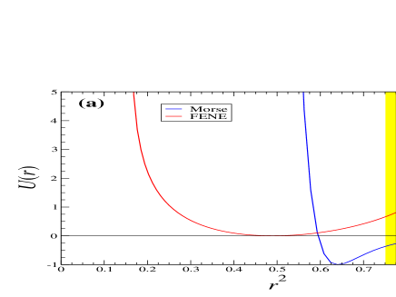
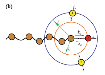
Figure 1: (a) Plots of bonded (FENE) and nonbonded (Morse) interactions used in the present model. The shaded area denotes distances where scission-recombination events may take place. (b) Two-dimensional projection of the living polymerization-depolymerization process with corresponding rates of polymerization $k_{p}$ and depolymerization $k_{d}$: chains consists of successively connected bonds, labeled by pointers. The pointers of end-bonds point to NIL (red particles). The breaking of a saturated bond ibond requires to set the pointers of the two connected bonds ibond and jbond = pointer(ibond) to NIL ( yellow particles, $2,\;4$). Setting $pointer(3)=1$ and $pointer(1)=3$ connects the end-monomer $imon=1$ and the individual reacting monomer $jmon=3$.

Using the assumption that no branching of chains is permitted, each bond is considered as a pointer, originating at a given monomer and pointing to the respective other bond with which the couple forms a nearest neighbor (brown particles), or to NIL (red particles), if the bond is free (unsaturated). The two possible bonds of each monomer imon are called ibond = imon and ibond = -imon. No specific meaning (or direction) is attached to the sign and this is merely a convenience for finding the monomer from the bond list: imon = $\arrowvert{\it ibond}\arrowvert$. Pointers are taken to couple independently of sign and the bonds are coupled by means of a pointer list in a completely transitive fashion.

In the LPB, only two simple operations are required for polymerization or depolymerization processes. Unsaturated bonds at chain ends point to NIL (nowhere) and only these bonds may recombine (pair) with the unsaturated bond of a free monomer. Therefore, the main difference with respect to EPs is that the monomer may attach or dissociate reversibly only to / from end-monomers of grafted LPB chains (following the model definition sketched in Figure 2) and no explicit distinction between the end-monomers, middle monomers or free monomers is required.

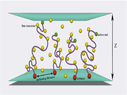
Figure 2: Schematic representation of the model LPB growth between two parallel plates. Polymer chains grow reversibly from the initiator molecules (red spheres) fixed on the impenetrable bottom wall. They are in thermal equilibrium with a reservoir of free monomers (gold spheres). We suppose that both the scission energy $J$ and the activation barrier are independent of the monomer position (along the chain contour as well as in space) and density. Desorption events occur only at the active chain ends (green spheres) and chains are not allowed to break along the backbone. Branching of chains is forbidden as well. The opposite im(semi)permeable wall is a bare surface at distance $z$ from the grafting plane.

As an example, Figure 3 shows snapshot pictures of LPB corresponding to mean chain length $\left<L\right>=32$ (left) and $\left\langle L\right\rangle=64$ (right) and grafting density $\sigma_{g}=1.0$. Each bond is described by a shifted FENE potential,

$$U_{\rm FENE}(l)=-K(l_{\rm max}-l_{0})^{2}\ln\left[1-\left(\frac{l-l_{0}}{l_{\rm max}-l_{0}}\right)^{2}\right]-J$$ (9)

where $\it J$ corresponds to the constant scission energy. Note that $U_{\rm FENE}\left(l=l_{0}\right)=-J$ and $U_{\rm FENE}$ near its minimum at $l_{0}$ is harmonic, with $K$ being the spring constant, and the potential diverges to infinity both when $l\rightarrow l_{\rm max}$ and $l\rightarrow l_{\rm min}=2l_{0}-l_{\rm max}$. Following Ref. Milchev2 , we choose the parameters $l_{\rm max}-l_{0}=l_{0}-l_{\rm min}=0.3$ and $K/k_{B}T=20$, $T$ being the absolute temperature. The units are such that the Boltzmann’s constant $k_{B}=1$. The nonbonded interactions between brush and free chain segments are described by the Morse potential, $r$ being the distance between the beads,

$$\frac{U_{M}\left(r\right)}{\epsilon_{M}}=\exp\left[-2\alpha\left(r-r_{\rm min}\right)\right]-2\exp\left[-\alpha\left(r-r_{\rm min}\right)\right]$$ (10)

with parameters $\alpha=24$, $r_{\rm min}=0.8$, and $\epsilon_{M}/k_{B}T$ standing for the strength of monomer-monomer interactions. In our present study we take typically $\epsilon_{M}/k_{B}T=0.2$ which corresponds to good solvent conditions since the $\Theta$-point of the coil-globule transition for a (dilute) solution of polymers described by the model, Eqs. 9 and 10, has been estimated Milchev4 as $k_{B}\Theta/\epsilon_{M}\approx 0.62$.

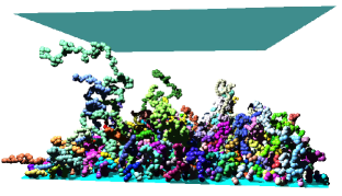
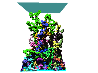
Figure 3: Snapshot picture of two LPB with $\sigma_{g}=1.0$, $\left<L\right>=32$ (left part) and $\sigma_{g}=1.0$, $\left<L\right>=64$ (right part) in their unperturbed states. The substrates are highlighted by cyan color, the opposite walls are in green color, while monomers of polydisperse brush belonging to short and long chains are displayed by different colors for more distinction. The ambient free monomers are not displayed for the sake of clarity. Only the shorter chains do sufficiently overlap and, hence, are somewhat stretched by the density gradient.

The model can be simulated fairly efficiently with a dynamic MC algorithm, as described previously Milchev3 ; Milchev4 . The trial update involves choosing a monomeric unit at random and attempting to displace it randomly by displacements $\Delta x,~{}\Delta y,~{}\Delta z$ chosen uniformly from the interval $-0.5\leq\Delta x,\Delta y,\Delta z\leq 0.5$. The transition probability for the attempted move is calculated from the $\delta U$ of the potential energies before and after the move as $W=\exp(-\Delta U/k_{B}T)$. Moves are then accepted according to the Metropolis criterion, if $W$ exceeds a random number uniformly distributed in the interval $\left[0,1\right)$ and one Monte Carlo Step (MCS) involves as many attempted moves as there are monomers in the system. In addition, during each MCS as many bonds as there are initiators in the system are chosen at random at the active ends of the grafted chains, and an attempt is made to break them according to the Metropolis algorithm. Attempts are also made to create new bonds between the end-monomers and free monomers within the potential range of $U_{M}$ (i.e., a new bond with energy $U_{\rm FENE}$).

In order to keep the system in equilibrium with the ambient phase of single free monomers and prevent the longer polymer chains from touching the top of the container, we have used a rather low value of the bond energy $J=2.0$. The lattice constant $s$ of the square grid of activated initiators is taken as a rule as $s=1$ for the case of a dense brush and, as a special case of a loose mushroom-like layer, $s=4$.

In $z-$direction the simulation box is bound by smooth (unstructured) impenetrable walls using the so called Weeks-Chandler-Andersen (WCA) potential, $U_{\text{WCA}}(r)$, (i.e., by the shifted and truncated repulsive branch of the Lennard-Jones potential), cf, Fig. 2,

$$U_{\text{WCA}}(r)=\begin{cases}4\epsilon\left[\left(\frac{r_{0}}{r}\right)^{12}-\left(\frac{r_{0}}{r}\right)^{6}\right]+\epsilon,&\text{for}~{}~{}r\leq 2^{1/6}r_{0}\\ 0,&\text{for}~{}~{}r>2^{1/6}r_{0}\end{cases}$$ (11)

which prevents particles from leaving the container. In Eq. (11) we set $r_{0}=1.0$. Thus, while the substrate plane is fixed at $z=0$, the top wall can be shifted in vertical direction like a piston to some desirable height $Z_{top}$ whereby all particles at distances closer than $Z_{top}-r_{0}$ to it are subject to repulsive force taken as the derivative of Eq. (11).

Typically, boxes of size $L_{x}\times L_{y}\times L_{z}$ and periodic boundary conditions in $x$ and $y$ directions have been used in the simulations with $L_{x}=L_{y}=16,32$ and $64\leq L_{z}\leq 256$ (all length in units of $l_{\max}$) for systems from $M_{t}=4096$ up to $32768$ monomers. Before starting to derive statistical averages, the grafted living polymer brush is equilibrated by MC method for a period of $10^{7}$ MCS (depending of the average chain length $\left<L\right>$ this period is varied) whereupon one performs 100 measurement runs, each of length $5\times 10^{7}$ MCS.

In order to calculate the force, resulting from compression of the LPB, the simulation starts with a well equilibrated in situ grown dense LPB ($\sigma_{g}=1.0$) containing chains of, say, $\left\langle L\right\rangle=32$ and the upper wall far enough above the top of the LPB so that it is not in contact with the brush. The wall is then gradually pushed down against the brush with different moving rates along a line normal to the grafting surface. After moving the wall to a specified distance from the grafting surface, the position of the wall is held fixed and measurements are carried out.

III.2 Homogeneous Monodisperse Polymer Brush (MPB)

In this case we also used the efficient off-lattice Monte Carlo method with the first monomer of each chain being rigidly fixed to grafting sites that are arranged regularly on a square lattice as shown in Figure 4 . The grafting surface is located at $z=0.0$, and a second non-adsorbing wall is put at $\it L_{z}$. The second wall is placed originally at a far enough distance from the grafting plane such that it does not affect the chain configurations for the chain length considered in the simulations. We study the system of polymer chains consisting of $N$ monomer with $N=32,~{}64$, and $128$ for the highest value of grafting density $\sigma_{g}=1.0$. Periodic boundary conditions were applied in the $xy$ direction. The brush was created in a fully stretched configuration and was then equilibrated over times much longer than the longest relaxation time $\tau_{R}$ of an single chain with excluded-volume interactions to obtain totally independent and relaxed start configuration for compression runs. It is well-known Gurler that for a chain with $N$ beads and under excluded-volume interactions, the largest (Rouse) relaxation time $\tau_{R}$ is given by, in units of $N$, $\tau_{R}\approx 0.25N^{2.19}$ in the absence of explicit solvent. In the monodisperse case, we have equilibrated the system for a time $\tau=10\tau_{R}\rm MCS$.

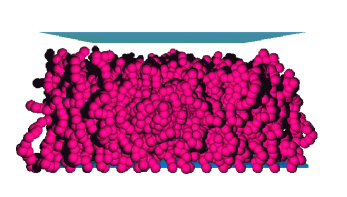
Figure 4: Snapshot of a MPB with chain length $N=32$ at grafting density $\sigma_{g}=1.0$ at equilibrium. Polymer chains are red, substrate atoms are cyan, and upper wall is green. Solvent particles are omitted for clarity.

Same as LPB system, in the MPB case, each bond is described by FENE potential where a bond of length $l$ has a maximum at $l_{max}=1.0$ (Eq. 9) and the nonbonded interaction between effective monomers is described by a Morse-type potential (Eq. 10).

IV Experimental studies

Materials. N-Isopropylacrylamide (NIPAAm, Aldrich, 97%) was purified by passing through an inhibitor removal column using a mixture of dichloromethane and hexane (v/v $\approx 1:1$) as the solvent and then recrystallized twice from a toluene/hexane solution (50% v/v) and dried under vacuum prior to use. Copper(I) bromide (CuBr, Aldrich, 98%) was purified by stirring in glacial acetic acid, filtering, and washing with ethanol three times, followed by drying in vacuum at room temperature overnight. Copper(II) bromide (Sigma-Aldrich, $\geq$ 99%), $N,N,N^{\prime},N^{\prime\prime},N^{\prime\prime}$-pentamethyldiethylenetriamine (PMDETA; 98%, Acros Organics), ethyl 2-bromoisobutyrate (E2Br-iB, 98%, Aldrich), (3-Aminopropyl)trimethoxysilane (APTMOS, 99%, Acros), bromoisobutyryl bromide (BIBB, 99%, Aldrich), and anhydrous toluene (Merck) were used as received. Milli-Q water (with a minimum resistivity of 18.2 M$\Omega$-cm) was obtained from a Millipore Direct-Q 5 ultrapure water system. THF for reactions and washings were dried by sodium before use. Double-sided polished silicon wafers (P-doped, (100)-oriented, 10-20 $\Omega$-cm resistivity, 0.56-mm thickness) were supplied by University Wafer Company (Boston, MA) and cut into $5\times 5\rm mm^{2}$ pieces using a Micro Ace Series 3 dicer (Loadpoint Ltd, England). Ultra-high-purity-grade argon was used in this study.

Initiator Synthesis. The ATRP initiator, 2-bromo-2-methyl-$N$-3-[(trimethoxysilyl)propyl]propanamide (BrTMOS), was synthesized using a procedure modified from literature Sun : To a stirred solution of APTMOS (1.79 g, 10 mmol) and triethylamine (1.01 g, 10 mmol) in 50 mL of dried THF, BIBB (3.45 g, 15 mmol) was added drop-wise at 0 ^∘C for 2 h under argon. The reaction was heated to room temperature and kept for 12 h with stirring and under argon protection. The precipitate was filtered off using a frit funnel. The product was a yellowish oil after the removal of the solvent. The product was redissolved with $\rm CH_{2}Cl_{2}$ (20 mL) and washed with 0.01 N HCl (2$\times$ 20 mL) and cold water (2$\times$ 20 mL), respectively. The organic phase was dried with anhydrous $\rm CaCl_{2}$. After the removal of the solvent, the final product was a colorless oil with a yield of 90.5%. ¹H NMR (300 MHz, $\rm CHCl_{3}$): 6.91 (s, 1H, NH), 3.49 (s, 9H, $\rm SiOCH_{3}$), 3.25 (t, 2H, $\rm CH_{2}N$), 1.95 (s, 6H, $\rm CH_{3}$), 1.68 (m, $\rm 2H,CH_{2}$), 0.67 (t, 2H, $\rm SiCH_{2}$). ¹³C NMR (600 MHz, $\rm CHCl_{3}$): 171.98, 62.57, 50.29, 42.62, 32.44, 22.52, 7.64.

Surface-initiated atom transfer radical polymerization (SI-ATRP). Silicon wafers were sonicated for $5$ min in ethanol and water, activated for $30$ min at $150$ ^∘C in piranha solution ($\rm H_{2}O_{2}$ (30 wt% in $\rm H_{2}O)/H_{2}SO_{4}$ (98 wt%), v/v $\approx 3:7$) (CAUTION: piranha solutions are strongly oxidizing and should not be allowed to contact organic solvent.) ,thoroughly rinsed with water and ethanol, dried in a stream of argon. A self-assembled monolayer (SAM) of the ATRP initiator was attached to the silicon wafer by immersion in a $10$ mM solution of BrTMOS in dry toluene at room temperature overnight. Next, the wafers were rinsed with anhydrous toluene, sonicated for $1$ min in acetone and in a water/$tert$-butanol mixture (v/v $\approx 1:1$), rinsed with water, dried in a stream of argon and transferred to the appropriate reactors for the polymerizations.

SI-ATRP of NIPAAm monomer was carried out at room temperature from a monolayer containing the SAM-Br initiator as follows: A mixture of MeOH/$\rm H_{2}O$ (v/v $\approx 1:1$) was degassed through four freeze-pump-thaw cycles before being introduced into the controlled atmosphere glove box. NIPAAm ($5.0$ g, $44$ mmol), CuBr ($40.0$ mg, $0.278$ mmol), $\rm CuBr_{2}$ ($\rm 14~{}mg$, $\rm 0.063~{}mmol$), and PMDETA ($175$ $\rm\mu L$, $0.835$ mmol) were dissolved in $30$ mL of MeOH/$\rm H_{2}O$ inside the glove box. The solution was then transferred via a cannula into a vial containing silicone wafer with uniform initiator SAM and sacrificial initiator E2Br-iB ($10$ $\rm\mu L$, $0.07$ mmol), and then vial was sealed and kept at room temperature for polymerization. After polymerization for a times ranging from $\rm 30~{}min$ to $\rm 120~{}min$, the substrate were removed from the vial and rinsed with copious amount of DI water, followed by sonication in EtOH and then $\rm H_{2}O$. After drying with a stream of argon, the samples were stored under Ultra-high-purity-grade argon.

AFM measurements. Force measurements were carried out with a NanoScope IIIa multimode atomic force microscope (Digital Instruments, Veeco-Bruker, Santa Barbara, CA, USA) equipped with a standard liquid cell on SI-ATRP grown PNIPAAm films in a liquid environment filled with deionized water. One micrometer in diameter $\rm SiO_{2}$ colloidal probe (Novascan Technologies, Inc., Ames, CA, USA) with a spring constant of $\rm 0.050~{}\pm~{}0.003~{}Nm^{-1}$ (determined using the thermal tune method) and a diameter of $\rm 1.00~{}\pm~{}0.006~{}\mu m$ (determined by a scanning a tip array) was used in the experiments. PNIPAAm coated wafer was placed on liquid cell and degassed DI water was injected into the cell and then the film was allowed to equilibrate for $\rm 1~{}hr$. The AFM cantilever was then set on top of the sample and started to move toward the sample surface with Z-ramp size of $\rm 2~{}nm$ and a dwell time of $\rm 100~{}ms$ per step. Cantilever deflection was recorded and averaged at each interval until tip-sample forces caused a deflection by $\rm 10~{}nm$, after which the cantilever was withdrawn from the surface in the same manner.

V SIMULATION RESULTS

As far as our main concern in this work is the comparison of experimentally measured compression force of a LPB with data, we mention very briefly some related results obtained from our Monte Carlo simulation. An interesting question thereby is to what extent the structure of the LPB meets theoretical predictions, mentioned in Section II. Therefore, in Figure 5(a) we present the observed density profiles of grafted monomers, $\phi(z)$, in an equilibrated LPB system at various temperatures after a $T$-quench from an initial equilibrium state at $k_{B}T=1.0$. It should be noted that all profiles are normalized to unity as $\int_{0}^{z}\phi(z)dz=1$. Evidently, in logarithmic coordinates, Figure 5b, one observes a power law decay of the density profiles, $\phi(z)\propto z^{-\alpha}$, manifested as a straight line, whereby the observed power $\alpha\approx 0.64$ at $T=1.0$ is shown to be in good agreement the theoretically expected one $\alpha\approx 2/3$ Milchev5 .

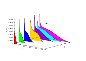
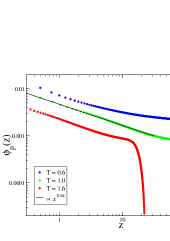
Figure 5: (a) Density profile of LPB, $\phi_{p}(z)$, at different temperatures (in units of $k_{B}T$) for LPB with total density of the system $\phi_{t}=0.5$ at $\sigma_{g}=1.0$. (b) Double logarithmic plot of density profiles at different temperatures, confirming the scaling behavior $\phi(z)\propto z^{-\alpha}$.

The data shown in Fig. 5 corresponds to equilibrated LPBs whereby the total monomer concentration in the container has been kept constant. We observe the same value of the exponent $\alpha$ when the temperature is further increased. Small deviations from the expected scaling behavior are found only during quenching of LPB chains to lower temperatures, Figure 5(b), for the higher $z$. We believe that this is probably due to single rather long chains which get repelled by the ceiling of the simulation container and bend backwards, increasing the local monomer density under the upper plane of the box. The reader may get impression about such effects from the snapshots shown in Fig. 6 where we display the variation of the average chain length $\langle L\rangle$ in a LPB with the total monomer concentration $\phi_{t}$.

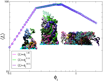
Figure 6: The average chain length $\langle L\rangle$ for a wide range of total monomer concentration $\phi_{t}$ confirming the scaling Eqs. 3 and 5. The three slopes correspond to dilute, semi-dilute, and concentrated regimes at $\sigma_{g}=1.0$. The observed slopes are $1.42,\;0.18,$ and $-0.51$ respectively. Sample snapshots belonging to each regimes are inserted in the plot.

The measured variation of the mean chain length $\langle L\rangle$ versus total monomer concentration, along with visual evidence from snapshots taken in the course of compositional variation, Figure 6, suggest the existence of several distinct regimes in terms of $\phi_{t}$. One may conclude from Figure 6 that the mean chain length of a LPB in a wide range of concentration is governed by a power-law relationships, confirming the scaling Eqs. (3) and (5) with exponents that differ from the predicted values for living polymers in bulk. Interestingly, at rather high concentrations the mean length $\langle L\rangle$ decreases with further growth of $\phi_{t}$, i.e., the LPB gets more compact as the longest chains are hindered in their growth due to the finite size of the simulation box. Thus, the polymerization process is shifted and this affects increasingly the many short chains living in the bottom. Clearly, more comprehensive investigation and increased computational efforts are needed to elucidate this aspect of the LPB behavior which we postpone for a separate publication.

V.1 Compression of in situ Grown LPB

In this section we examine the interaction between a LPB chains immersed in a good solvent and a test surface using coarse-grained off-lattice Monte-Carlo simulations. Our purpose is to obtain force-displacement curves for the penetration of such an AFM tip (test surface) into a polydisperse chains of LPB as a function of layer characteristics. To this end, the test surface is

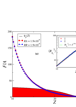
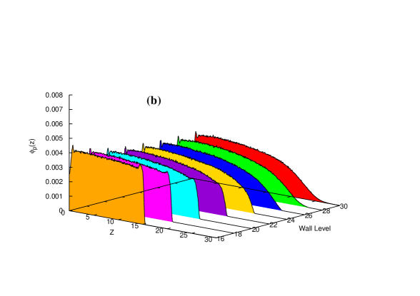
Figure 7: (a) Force-displacement curves for relaxed MPB with grafting density $\sigma_{g}=1.0$ and chain length $N=32$ during the loading $\Downarrow$ and unloading $\Uparrow$ process at $k_{B}T=1.0$. The rates of approaching and retraction as unit of ${\rm MCS}^{-1}$ are given as parameter. The inset shows a plot of the mean squared gyration radius component $\left\langle R_{g_{z}}^{2}\right\rangle$ in direction perpendicular to the grafting surface vs height of the mobile compressing surface (repulsive wall) during loading and unloading. (b) Density profile of MPB, $\phi_{p}(z)$, for different wall positions in the loading experiment.

represented either as an impenetrable or as semi-permeable surface, consisting of a long cylinder of cross-section area $A$. The interaction between a LPB and a AFM tip can easily be simulated by a slight variation of the algorithms used to study forces between two test surfaces in which one of them bears an end-grafted polymer brush. In the simulations results given below, we assumed a repulsive force between the monomers and the surface Murat3 , taken as a Weeks-Chandler-Andersen potential, i.e. as the repulsive (and shifted) branch of a Lennard-Jones potential. One might also use a Lennard-Jones with an attractive short-range components Grest3 ; Grest4 . Both of these forces gave qualitatively similar results.

For the sake of comparison, we also simulated an equilibrated monodisperse polymer brush (MPB) containing chains of equal length $N=32$ at high grafting density $\sigma_{g}=1.0$. Originally, the mobile wall is far enough so that it is not in contact with the brush. To simulate the loading and unloading processes of wall, we move it downwards at rate $RA$, and then up at retraction rate $RR$, measured as distance per time units of MCSteps.

Figure 7(a) shows the results of the force-displacement curve for an equilibrated high density MPB at vanishing rates $RA=RR=1.9\times 10^{-6}$. The force $F$ is normalized by the area $A$ of contact and describes thus the pressure on the wall. As shown in the main panel of Figure 7(a), during the loading from $z_{i}=30$ to $z_{f}=10$, the tip goes into the sample down to a depth $\delta=z_{f}-z_{i}$, causing deformation of the brush. During the wall retraction, it goes back from $z_{f}=10$ to $z_{i}=30$. Since the rate of approaching and retraction at well equilibrated conditions are negligible, the MPB behaves as an elastic material and regains step by step its own shape, exerting equal pressure on the wall. The $F$ vs $z$ curves for the approaching / retracting wall lie on top of each other and are virtually indistinguishable. Therefore, during such an “infinitely“ slow loading and unloading one observes no hysteresis in the force - height relationship. In the inset to Figure 7(a) we plot the mean squared gyration radius component $\left\langle R_{g_{z}}^{2}\right\rangle$ in direction perpendicular to the grafting surface as function of the wall position. Evidently, in logarithmic coordinates these transients appear as straight lines, suggesting that the height of the perturbed MPB changes by a power law, $\left\langle R_{g_{z}}^{2}\right\rangle\propto z^{\alpha}$, whereby the observed power $\alpha\approx 1.96$, i.e. $h\propto z$ for $z<30$.

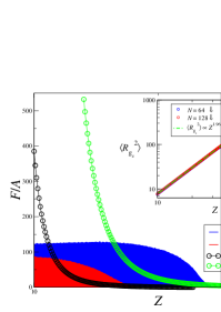
Figure 8: Comparison between force-displacement curves of two relaxed MPB with grafting density $\sigma_{g}=1.0$ and chain length $N=64$ and $N=128$ in the loading experiment $\Downarrow$. The density profile (shaded area) is included for comparison. The inset shows the same trend for $\left<R_{g_{z}}^{2}\right>$ as $N=32$.

In Figure 7(b), we show the monomer distribution of the MPB along the $z$-direction at different piston positions (wall level) during the loading experiments. As can be seen from Figure 7(b), the histograms follow indeed the parabolic characteristics of ”dead“ monodisperse brushes Winehold in the beginning of the process (nearly unperturbed state) while at stronger compression, for $z\leq 22$, the histograms indicate a flat uniform distribution of matter in the compressed MPB. Eventually, one ends up with a rather sharply peaked $\phi_{p}(z)$ (not included for the sake of clarity) near the grafting surface, characterizing a “proximal zone” with density oscillations typical for all fluids “packed” in the vicinity of a hard wall.

In the main panel of Figure 8 we compare the pressure of grafted monomers along direction $z$, normal to the grafting surface for two MPBs with chain lengths $N=64$ and $N=128$, both at highest grafting density, i.e., $\sigma_{g}=1.0$. The density profiles are included for the sake of comparison. It becomes evident from Figure 8 that both simulations demonstrate a qualitatively similar behavior to that of picture Figure 7. In the inset to Figure 8 one may see the same scaling of mean squared gyration radius component $\left\langle R_{g_{z}}^{2}\right\rangle$ in direction perpendicular to the grafting surface as in Figure 7(a), whereby the force-displacement curves again collapse on a single master curve. This behavior is characteristic for large tip AFM experiments Subramanian . Because of the large grafting density and the excluded-volume interactions, the chains are strongly stretched and resemble rods with small probability for the chains to escape compression by moving away from the test surface.

In Figure 9, a force-displacement approach curve obtained for LPB system with $\left\langle L\right\rangle=32$ is compared to the equivalent MPB with length $N=32$ of the grafted chains. For both cases the data corresponds to polymer brushes at their highest grafting density, i.e., $\sigma_{g}=1.0$. For better interpretation, the resulting brush profiles are also included in the main panel of Figure 9 by shaded area. It is common to define the layer thickness $\langle z\rangle$ of a MPB as the first moment of the monomer density profile $\phi_{p}(z)$, i.e., the average distance of a chain monomer from the surface

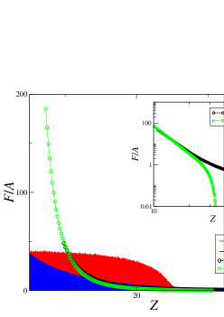
Figure 9: Force-displacement curves of relaxed LPB and MPB in loading experiment for $\left\langle L\right\rangle=32$ (LPB) and $N=32$ (MPB) at $\sigma_{g}=1.0$. The rate of wall displacement is $RA=1.9\times 10^{-6}$ for both LPB and MPB.

$$\langle z\rangle=\frac{2\int z\phi_{p}(z)dz}{\int\phi_{p}(z)dz}$$ (12)

The equilibrium profile of such a monodisperse “dead” brush is more compact with a steeper slope near $z\approx\langle z\rangle$, than that of the analogous LPB system (as shown in Figure 9) which goes to far larger $z$. In agreement with the theoretical predictions Milner4 , cf., Section II, it is seen from Figure 9 that the weak compression force of the LPB exceeds significantly the one due to MPB.

At large compression ($z<\langle z\rangle=22.75$) or small separations, of course, the two force-displacement relations are indistinguishable. The pressure in this limit is exerted by the uniform density of the compressed brush suggesting that the repulsive force is well approximated by the corresponding osmotic pressure of a non-grafted semidilute solution. Hence the two interaction forces become identical when the MPB height $\langle z\rangle=22.75$ is much less than the average chain length $\langle L\rangle=32$ of the corresponding LPB case.

For small compressions ($z\approx\langle z\rangle=22.75$), the force-displacement curve of the MPB vanishes abruptly in contrast to the equivalent LPB case (see inset to Figure 9). This important distinction is due to the existence of few much longer chains in the LPB. Therefore, the reactive force of a LPB extends to larger separations and the simulation predicts a non-vanishing force at $z>\langle z\rangle=22.75$.

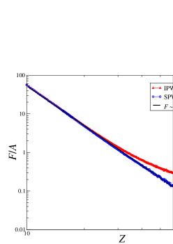
Figure 10: Comparison between force-displacement curves of relaxed LPB, obtained with both impermeable and semi-permeable wall for $\left\langle L\right\rangle=32$ at $\sigma_{g}=1.0$.

In order to be as close as possible to real applications of LPB, in which a LPB is subjected to force measurement either by AFM or SFA instruments, we also examined the case of a semi-permeable wall (SPW) as opposed to that of completely impenetrable rigid wall (IPW). With a SPW, a complete equilibration of the whole LPB takes place under conditions when the unreacted single monomers may move freely through the wall and enter the volume above it. In this way the monomer concentration under the moving wall is not affected by the wall motion and remains equal to that in the whole volume regardless of the wall position as is the case with an AFM tip. Otherwise, any change in the wall position would have induced a change in the average chain length $\langle L\rangle$ because of growing $\phi_{t}$, according to Eq. (5) and, therefore, also in the reactive force of the LPB even before the wall gets in touch with the brush. With other words, any variation of an impenetrable wall would produce an essentially different LPB which precludes a meaningful study of the force - wall position relationship at fixed monomer concentration $\phi$. In order to avoid inaccuracies and in view of the additional time the monomers need to move through the SPW, we chose in this case the equilibration periods twice longer than in the IPW case with rate in the range of $10^{-8}-10^{-10}$.

The result of such simulation for force-displacement curve in loading experiment is shown in Figure 10, together with the curve for the same LPB, compressed by an IPW of identical area. The average chain length in both cases is $\langle L\rangle=32$ and the grafting density is $\sigma_{g}=1.0$. The force exerted by the LPB on the SPW excludes the interaction between non-grafted monomers and the test surface. One can immediately see that the SPW clearly gives a weaker force compared to that with IPW at small compressions. This difference becomes indistinguishable at lower separation or large degrees of compression, and the curves in both cases superimpose perfectly for $z\leq 20$ as expected. It is evident from Figure 10 that the force-displacement curves appear as straight lines in logarithmic coordinates, suggesting a power law scaling, $F\propto z^{-\alpha}$, where the observed exponent $\alpha\approx 3.4$ is shown to describe a dense LPB system both in the SPW and IPW case.

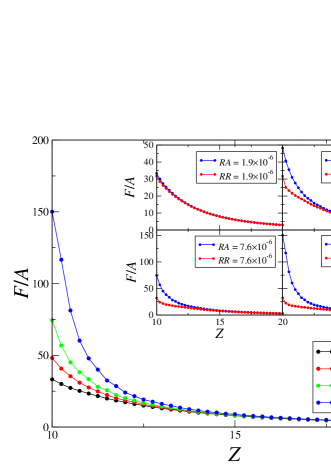
Figure 11: The effect of moving velocity of the test wall on the force - displacement curve of LPB with $\langle L\rangle=32$ and $\sigma_{g}=1.0$ during the loading process. In the inset a detailed view of the force hysteresis during loading and unloading experiments for a LPB is shown. Results for four incoming and retraction velocities are included, as indicated.

Eventually, in Figure 11 we present the effects of tip scan rate on the hysteresis behavior in the force-displacement curve during a loading/unloading experiment. Recently, the response of a compressed monodisperse polymer brush as function of $\sigma_{g}$ and compression rate $RA/RR$ was studied by Brownian Dynamics simulation Elvingson . Our simulations for a LPB system are performed with an average chain length $\langle L\rangle=32$ and grafting density $\sigma_{g}=1.0$. The main panel of Figure 11 shows the observed force-displacement curve in loading experiments for different indentation/compression rate. Evidently, as the scan rate gets faster, the final values of the response force at small separations $z<15$ grow while the superposition region is shifted to lower compressions. These predictions are found to agree well with experimental interpretations of Hoh and Engel Hoh in their AFM indentation test even though our approaching rates are about three order of magnitude smaller than in a real AFM indentation experiment. In the inset plots of Figure 11 one may see the hysteresis becomes stronger with increasing loading / unloading rate which reflects also growing energy dissipation given by the enclosed area of the indentation and retraction curves. The values of energy dissipation has been measured experimentally for different systems Treventhan . As can be seen from the Figure 11, by decreasing the scan rate the hysteresis may be completely eliminated when full equilibrium is reached without energy dissipation. The latter shows an elastic behavior of a thin layer in which the material can regains step by step its own shape during the withdrawal process Lee .

In practice, the sample may loose elasticity in the process of compression so that when the tip is withdrawn, it does not regain immediately its former shape. The load gradually decreases whereas the penetration depth stays the same. Hence indentation and retraction curves seldom overlap. At a given penetration depth the force of the unloading curve is smaller than the force at loading. This difference between the indentation and the withdrawal force curves appears as a “loading-unloading hysteresis”. The hysteresis may lead to an incorrect determination of displacements and, in particular, because of the hysteresis, the load in the loading curve for a given displacement may appear bigger and finally overcome those of the unloading curve. Experimentally, Hoh and Engel Hoh have shown that the loading/unloading hysteresis is scan rate- (or, velocity)-dependent. At high scan rates the separation between the contact lines in indentation and retraction modes is large and a considerable hysteresis appears. As the scan rate is decreased, the system has more time to recover and this separation reaches a minimum so that the hysteresis becomes smaller and may vanish.

VI Comparison Between Experiment and Simulation

Here we focus on the comparison of our simulations exclusively with own AFM-based, colloidal probe compression measurements. PNIPAAm brush was grafted on the surface of a self-assembled monolayer containing the initiator, using surface-initiated atom transfer radical polymerization (ATRP). Varying the reaction time and monolayer initiator concentration controlled the molecular weight and grafting density, respectively. For details on the synthesis of PNIPAAm brush samples and evaluation of grafting density see Supporting information. AFM measurements were performed on ATRP grown PNIPAAm films in a standard fluid cell containing deionized water as a good solvent at $26~{}{\rm C^{\circ}}$ which was below the LCST temperature of PNIPAAm.

Experimentally, a surface force apparatus (SFA) was used by Zhu et. al.,Zhu and Plunket et. al.,Plunket to measure the force encountered between tethered poly(N-isopropylacrylamide) (PNIPAAm) at, below, and above lower critical solution temperature (LCST) and plain mica surfaces and mica surfaces coated with lipid bilayers. In the SFA technique, the force of interaction between two perpendicular crossed cylinders can be measured as a function of the distance between the two cylindrical surfaces. Plunkett et. al.,Plunket coated the surface of one cylinder with terminally anchored PNIPAAm and kept the surface of the other cylinder bare.

In our simulation, force was measured between a LPB and a wall, taken either as a hard impenetrable, or a semi-permeable layer, and compared to experimental data obtained for PNIPAAm under good solvent condition (below LCST) as well as to the simulation results for monodisperse MPB case. This comparison makes sense only when the length of chains in the MPB brush, $N$, is equal to the mean chain length $\langle L\rangle$ of the LPB. However, for a living polymer $\langle L\rangle$ depends essentially on the concentration of free monomers in the container Wittmer2 , and in the case of impenetrable wall will therefore change dynamically with the variation of monomer concentration as the wall is moved with respect to the grafting plane. To prevent this and examine solely the effect of polydispersity at equal length of the chains in both LPB and MPB brush, we use in our simulation also a semi-permeable wall that is impenetrable for the grafted polymers yet completely permeable for the single non-polymerized monomers. These monomers can then move freely through the mobile wall and thus keep the total concentration in the box constant.

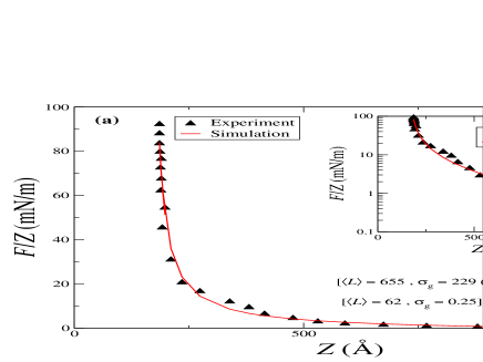
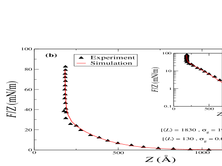
Figure 12: (a) Normalized force of Plunkett et. al.,Plunket for $\langle L\rangle^{\rm exp}=$ 655 plotted vs the distance between untreated mica and a PNIPAM brush polymerized at grafting density $229$ Ų/chain and comparing to simulated interaction force for a given grafting density and degree of polymerization, as indicated. (b) Same as (a) but for $\langle L\rangle^{\rm exp}=1830$, grafting density $1930$ Ų/chain and simulated interaction force for a different set of grafting density and degree of polymerization, as indicated.

Figure 12 illustrates the starting point of our analysis: from the data presented by Plunkett et. al., Plunket for a range of end grafted PNIPAM polymers that were synthesized by living polymerization (ATRP) on a gold flat surface with different grafting density (${\sigma_{g}}^{\rm exp}$) and degree of polymerization ($\left<L\right>^{\rm exp}$), we can identify a number of choices (${\sigma_{g}}^{\rm exp}$, $\left<L\right>^{\rm exp}$) where a quantitatively precise mapping of the experimental force-displacement curve on the simulated interaction force, for carefully chosen pairs of parameters (${\sigma_{g}}^{\rm sim},\left<L\right>^{\rm sim}$), is possible. Here we use subscripts “exp” and “sim” to distinguish the real experimental data from their simulation counterparts, respectively. Thus, apart from suitable adjustment of pair parameters, the length scale of the simulation (i.e., the lattice spacing) $s$ is adjusted to physical units by requiring that

$$\left(\frac{s}{2\left<R_{F}^{2}\right>^{1/2}}\right)^{\rm exp}=\left(\frac{s}{2\left<R_{F}^{2}\right>^{1/2}}\right)^{\rm sim}$$ (13)

The results of this fitting process for two experimentally calculated values $\left({s}/{2\left<R_{F}^{2}\right>^{1/2}}\right)=0.033$ and $0.046$ (obtained by Plunkett et. al. Plunket ) are shown in Figure 12. As can be seen from the figure, a good fit over the entire range of separations $z$ is obtained for $\left<L\right>=62$ and $\sigma_{g}=0.25$ in case (a) and for $\left<L\right>=130$ and $\sigma_{g}=0.0625$ in case (b). The corresponding experimental values for $\left<L\right>$ and $\sigma_{g}$ are indicated in the figure. It should be noted, from experimental point of view, that all experimentally determined grafting densities are sufficiently high Plunket so that the excluded volume interactions make the chains extend away from the substrate and form a brush structure. Therefore, the selected experimental grafting density for the comparison with simulated data at $\phi=0.5$ (which corresponds to semi-dilute brush regime in the simulation) confirmed that the experimentally synthesized grafted layer is in the genuine brush regime.

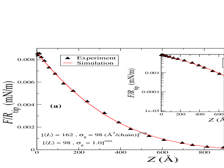
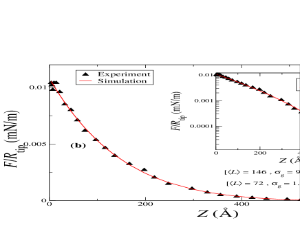
Figure 13: (a) Normalized force for $\langle\it{L}\rangle^{\rm exp}=$ 162 plotted vs the distance between AFM colloidal tip and a PNIPAM brush polymerized at grafting density $98$ Ų/chain and comparing to simulated interaction force for a given grafting density and degree of polymerization, as indicated. (b) Same as (a) but for $\langle L\rangle^{\rm exp}=146$, grafting density $98$ Ų/chain and simulated interaction force for a different set of grafting density and degree of polymerization, as indicated.

Bearing in the mind that the self-similar character of the conformation of the chains allows for some arbitrariness of the scales, one has to do an explicit mapping of a coarse-grained model of a flexible linear polymer either in grafted or non-grafted form on the real material. The principles of this mapping originate from the assumed general shape of the free energy of a chain $f_{p}$, when one compares it with the properties of ideal chains in good solvents with an end-to-end distance $R$. The free energy of a single chain for a regular solution is obtained by inserting the excluded volume contribution $f_{p}^{e}$ and entropic component $f_{p}^{s}$ into the equation $f_{p}=f_{p}^{e}+f_{p}^{s}$. The excluded volume contribution to the free energy of a single chain is obtained by integration over the occupied volume, hereby calculating the average over the all conformations

$$f_{p}^{e}=\frac{1}{2}\int kT\upsilon_{e}\left<c_{m}^{2}\left(\bf r\right)\right>d^{3}\bf r$$ (14)

where $\left<c_{m}^{2}(\bf r)\right>$ is square average local monomer density and $\upsilon_{e}$ is excluded volume interaction parameter. If we choose for the description of the mean local density $\left<c_{m}\left(\bf r\right)\right>$ a Gaussian function, with a radius of gyration $R_{g}$, we obtain

$$f_{p}^{e}=\frac{kT}{2}\upsilon_{e}N^{2}\left(\frac{3}{4\pi R_{g}^{2}}\right)^{3/2}$$ (15)

Eventually, one may choose the ideal state with vanishing excluded volume forces and coil size in thermal equilibrium $R_{0}$, where $R_{g}=R_{g,0}$ and $R_{0}^{2}=a_{0}^{2}N$, and replace $R_{g}$ by $R$ assuming $R\sim R_{g}$. Thus one may express $f_{p}^{e}$ as

$$f_{p}^{e}=\frac{kT}{2}3^{3/2}\psi\left(\frac{R_{0}}{R}\right)^{3}$$ (16)

The parameter $\psi=\left(3/2\pi\right)^{3/2}\left(\upsilon_{e}/a_{0}^{4}\right)R_{0}$, is dimensionless and determines the excluded volume energy associated with a single chain.

A further requirement is that one needs an expression to take into account the conformational entropy indicating the elastic force built up on a coil expansion. This equation yields the second part of the free energy, $f_{p}^{s}$, and is given by

$$f_{p}^{s}\approx kT\left(\frac{R}{R_{0}}\right)^{2}$$ (17)

Finally, combination of the Eqs. (16) and (17) yields the free energy of a chain as a function of $R$. One may determine the important relation between $R_{F}$ and the degree of polymerization $N$ by calculating the equilibrium value of $R$ at the minimum of the free energy $f_{p}$, where $df_{p}/d(R/R_{0})=0$. $R_{0}$ is the coil size in thermal equilibrium. This leads to the relation $R\simeq\left(\nu_{e}/a_{0}^{4}\right)^{1/5}R_{0}^{6/5}=\left(\nu_{e}a_{0}^{2}\right)^{1/5}N^{3/5}$. One may identify $R$ with the Flory radius $R_{F}$ and it can be represented thus as $R_{F}=a_{F}N^{3/5}$ with $a_{F}\backsimeq\left(\nu_{e}a_{0}^{2}\right)^{1/5}$.

The scaling law Eq. (13) is indeed in full accord with experiments (e.g., see ref 94) and it can be used for the translation of experimental findings to results of simulation in the case of various expanded polymer system in a good solvent. Of particular interest, we applied the same criteria in order to map our coarse-grained level simulations of force-displacement curve of a LPB to the experimental results obtained by SFA experiment (see Figure 12) and own colloidal probe AFM analysis on PNIPAAm brush in the good solvent. Since in the case of LPB system, there is only a single factor relating the length scale of the simulation to the real length scale and leads to a mapping process that conserves the chain conformation during translation, it can be expected that the precise description of coarse-grained model for force-displacement curve in Figure 12 is restricted to special cases. As an example, Figure 13 presents the force-displacement behavior in a AFM analysis for the pairs ($\left<L\right>=162,~{}\sigma_{g}=98$ Ų/chain)^exp, and ($\left<L\right>=146,~{}\sigma_{g}=98$ Ų/chain)^exp. All force data are normalized by the colloidal tip radius $R_{\rm tip}$. As can be seen from Figure 13, we find the closest corresponding translated pairs in simulation data as ($\left<L\right>=98,~{}\sigma_{g}=1.0$)^sim, and ($\left<L\right>=72,~{}\sigma_{g}=1.0$)^sim. The inset in Figure 13(a) shows that for very small compressions, the semi-log plot of the force-displacement curve deviates somewhat from the coarse-grained model and near $z\approx 900$ Å the simulation curve $\left<L\right>^{\rm sim}=98$ slightly underestimates the experimental data. As shown in the inset to Figure 13(b), in the case of lower degree of polymerization, $\left<L\right>^{\rm sim}=72$, the same deviation is also observed for lower separations while the underestimation is slightly decreased.

VII CONCLUSIONS

In the present work we have studied and tried to reproduce the force exerted by a LPB chains on a test surface. Our studies have been carried out by means of an efficient off-lattice Monte Carlo algorithm. To this end comprehensive Monte Carlo simulations of the properties of a LPB made of flexible living polymer chains under good solvent conditions have been carried out. Most of our studies consider moderate and high grafting densities of the chains whereby the ensuing polymer brush may be classified as strongly stretched.

An examination of the static properties of such LPB suggests that the observed monomer density profiles reveal power-law decline of the density $\phi(z)$ with increasing distance $z$ perpendicular to the grafting plane, $\phi(z)\propto z^{\alpha}$ with $\alpha\approx 0.64$ which is very close to the theoretically predicted value of $\alpha=2/3$ for diffusion-limited aggregation Wittmer1 . The probability distribution $c(N)$ of chain lengths $N$ in the strongly polydisperse living polymer brush is also found to follow a power law relationship, $c(N)\propto N^{-\tau}$, which qualitatively differs from the exponential Flory-Schulz Molecular Weight Distribution typical for living polymers in the bulk. The observed value of $\tau\approx 1.70$ is again rather close to the value of $\tau=7/4$, predicted for the case of “needle growth“ (Diffusion-Limited Aggregation Without Branching) Wittmer1 , except for cases of rather short LPBs, grown at high temperature $T>1.0$, where the chains do not stretch strongly and an exponential MWD is observed. One may thus conclude that the static properties of a LPB at equilibrium are very different from those of a semi-dilute or dense solution of living polymers in the bulk, and are governed by different laws.

One of the main concerns of this work has been the study of the force, exerted by a LPB on a test surface, and the comparison of simulational data with that from our own and other laboratory experiments. We have compared the force-displacement behavior from the set of experiments Plunket , obtained by SFA analysis on PNIPAAm brush under good solvent condition at temperature below LCST of PNIPAAm (Figure 12), and also our own experimental results obtained by colloidal probe AFM measurements on PNIPAAm brush at same conditions of SFA (Figure 13) with data from the present simulation. Generally, by adjusting the conformational parameter $s/2\langle R_{F}^{2}\rangle^{1/2}$ and the conversion factor from model lattice spacings to realistic nanometer scale, we find an almost perfect agreement. Small deviations between simulation results and experiment are only found for weak compression where in the case of SFA measurements, the simulation slightly overestimates the data and in the case of AFM experiments, the simulation slightly underestimates them.

It is clear, however, that more work is needed until full understanding of the properties of living polymer brushes, obtained by ATRP is achieved. Especially interesting and unexplored is the problem of LPBs, grown on curved surfaces, including the corresponding force-distance relationship which we see as our next target for research.

Supporting Information Available

Full details of the experimental characterization used in this study are provided as a file in Supporting Information. This material is available free of charge via the Internet at http://pubs.acs.org.

Table of Contents Graphic:
”Dynamic Compression of in situ Grown Living Polymer Brush: Simulation and Experiment”,
by K. Jalili, F. Abbasi, and A. Milchev K. Jalili^1,2, F. Abbasi², A. Milchev

References

- (1) Dyer, D. J. AdV. Funct. Mater. 2003, 13, 667.
- (2) Gates, B. D.; Xu, Q.; Stewart, M.; Ryan, D.; Willson, C. G.; Whitesides, G. M. Chem. ReV. 2005, 105, 1171.
- (3) Kawaguchi, M.; Takahashi, A. AdV. Colloid Inter. Sci. 1992, 37, 219.
- (4) Binnig, G.; Quate, C. F. Phys. ReV. Lett. 1986, 56, 930.
- (5) Magonov, S. N.; Reneker, D. H. Annu. ReV. Mater. Sci. 1997, 27, 175.
- (6) García, R.; Pérez, R. Surf. Sci. Rep. 2002, 47, 197.
- (7) Kaholek, M.; Lee, W.-K.; LaMattina, B.; Caster, K. C.; Zauscher, S. In Polymer Brushes; Advincula, R. C., Brittain, W. J., Caster, K. C., Rühe, J., Eds.; Wiley-VCH: Weinheim, Germany, 2004; pp 381.
- (8) Wilder, K.; Quate, C. F.; Singh, B.; Alvis, R.; Arnold, W. H. J. Vac. Sci. Technol. B 1996, 14, 4004.
- (9) Halperin, A.; Tirrell, M.; Lodge, T. Adv. Polym. Sci. 1992, 100, 31.
- (10) Klein, J. Annu. Rev. Mater. Sci. 1996, 26, 581.
- (11) Szleifer, I.; Carignano, M.A. Adv. Chem. Phys. 1996, 94, 165.
- (12) Grest, G. S. Adv. Polym. Sci. 1999, 138, 149.
- (13) Binder, K.; Kreer, T.; Milchev, A. Soft Matter 2011, 7, 5669.
- (14) Napper, D. H. Polymeric Stabilization of Colloidal Dispersions; Academic Press: London, 1983.
- (15) Hamilton, W. A.; Smith, G. S.; Alcantar, N. A.; Majewski, J.; Toomey, R. G.; Kuhl., T. L. J. Polym. Sci., Part B: Polym. Phys. 2004, 42(17), 3290.
- (16) Pastorino, C.; Binder, K.; Kreer, T.; Muller, M. J. Chem. Phys. 2006, 124(6), 064902.
- (17) Klein, J.; Kumacheva, E.; Mahalu, D.; Perahia, D.; Fetters, L. J. Nature 1994, 370(6491), 634.
- (18) Auroy, P.; Auvray, L.; Léger, L. Phys. Rev. Lett. 1991, 66(6), 719.
- (19) Alexander, S. J. Phys. 1977, 38, 983.
- (20) Milner, S. T.; Witten, T. A.; Cates, M. E. Macromolecules 1988, 21(8), 2610.
- (21) Milner, S. T.; Witten, T. A.; Cates, M. E. Europhys. Lett. 1988, 5(5), 413.
- (22) Halperin, A.; Zhulina, E. B. Macromolecules 1991, 24(19), 5393.
- (23) Biesheuvel, P. M. J. Colloid Interface Sci. 2004, 275(1), 97.
- (24) Biesheuvel, P. M.; de Vos, W. M.; Amoskov, V. M. Macromolecules 2008, 41(16), 6254.
- (25) de Gennes, P. G. Macromolecules 1980, 13(5), 1069.
- (26) Wijmans, C. M.; Scheutjens, J. M. H. M.; Zhulina, E. B. Macromolecules 1992, 25(10), 2657.
- (27) Auroy, P.; Mir, Y.; Auvray, L. Phys. Rev. Lett. 1992, 69(1), 93.
- (28) Cho, J.-H. J.; Smith, G. S.; Hamilton, W. A.; Mulder, D. J.; Kuhl, T. L.; Mays, J. Rev. Sci. Instrum. 2008, 79(10), 103908.
- (29) Smith, G. S.; Kuhl, T. L.; Hamilton, W. A.; Mulder, D. J.; Satija, S. Physica B: Condensed Matter 2006, 385-386 (Part 1), 700.
- (30) de Vos, W. M.; Biesheuvel, P. M.; de Keizer, A.; Kleijn, J. M.; Cohen Stuart, M. A. Langmuir 2008, 24(13), 6575.
- (31) de Vos, W. M.; Biesheuvel, P. M.; de Keizer, A.; Kleijn, J. M.; Cohen Stuart, M. A. Langmuir 2009, 25(16), 9252.
- (32) Grest, G. S. J. Chem. Phys. 1996, 105(13), 5532.
- (33) Murat, M.; Grest, G. S. Macromolecules 1989, 22(10), 4054.
- (34) Lai, P. Y.; Zhulina, E. B. Macromolecules 1992, 25(20), 5201.
- (35) Lai, P.-Y.; Binder, K. J. Chem. Phys. 1992, 97(1), 586.
- (36) Lai, P.-Y.; Binder, K. J. Chem. Phys. 1993, 98(3), 2366.
- (37) Neelov, I. M.; Binder, K. Macromol. Theory Simul. 1995, 4(1), 119.
- (38) Neelov, I. M.; Borisov, O. V.; Binder, K. Macromol. Theory Simul. 1998, 7(1), 141.
- (39) Neelov, I. M.; Borisov, O. V.; Binder, K. J. Chem. Phys. 1998, 108(16), 6973.
- (40) He, G.-L.; Merlitz, H.; Sommer, J.-U.; Wu, C.-X. Macromolecules 2007, 40(18), 6721.
- (41) Coluzza, I.; Hansen, J.-P. Phys. Rev. Lett. 2008, 100, 016104.
- (42) Seidel, C.; Netz, R. R. Macromolecules 2000, 33(2), 634–.
- (43) Kreer, T.; Metzger, S.; Muller, M.; Binder, K.; Baschnagel, J. J. Chem. Phys. 2004, 120(8), 4012–4023.
- (44) Dimitrov, D. I.; Milchev, A.; Binder, K. J. Chem. Phys. 2006, 125(3), 034905.
- (45) Dimitrov, D. I.; Milchev, A.; Binder, K. J. Chem. Phys. 2007, 127(8), 084905.
- (46) Milner, S. T. Science 1991, 251, 905.
- (47) Milner, S. T. Europhys. Lett. 1988, 7, 695.
- (48) Jeon, S. I.; Lee, J. H.; Andrade, J. D.; Gennes, P. G. D. J. Colloid Interface Sci. 1991, 142, 149-158.
- (49) Jeon, S. I.; Andrade, J. D. J. Colloid Interface Sci. 1991, 142, 159-166.
- (50) Subramanian, G.; Williams, D. R. M.; Pincus, P. A. Macromolecules 1996, 29, 4045-4050.
- (51) McCoy, J. D.; Curro, J. G. J. Chem. Phys. 2005, 122, 164905.
- (52) Steels, B. M.; Koska, J.; Haynes, C. A. J. Chromatogr. B 2000, 743, 41-56.
- (53) Pang, P.; Koska, J.; Coad, B. R.; Brooks, D. E.; Haynes, C. A. Biotechnol. Bioeng. 2005, 90, 1-13.
- (54) Flory, P. J. Principles of Polymer Chemistry; Cornell University Press: Ithaca, NY, 1953.
- (55) Wheeler, J. C.; Pfeuty P. Phys. Rev. Lett. 1981, 46, 1409.
- (56) Pfeuty P.; Wheeler J. C., Phys. Lett. 1981, A 84, 493.
- (57) Wittmer, J. P.; Milchev, A.; Cates, M. E. J. Chem. Phys. 1998, 109, 834.
- (58) Cates, M. E.; Candau, S. J. J. Phys.: Condens. Matter 1990, 6869.
- (59) Vidal, A.; Guyot, A.; Kennedy, J. P. Polym. Bull. (Berlin) 1982, 6, 401-407.
- (60) Advincula, R. C.; Brittain, W. J.; Caster K. C.; Rühe, J. (eds.) Polymer Brushes: Synthesis, Characterization, Applications 2004 Wiley-VCH, Weinheim
- (61) Wittmer, J. P.; Cates, M. E.; Johner, A.; Turner, M. S. Europhys. Lett. 1996, 33, 397.
- (62) Witten, T. A.; Sander, L. M. Phys. Rev. B 1983, 27, 5686.
- (63) Guiselin, O. Europhys. Lett. 1992, 17, 225.
- (64) Meakin, P. Phys. Rev. A 1986, 33, 3371; Krug, J.; Kassner, K.; Meakin, P.; Family, F. Europhys. Lett. 1993, 24, 527.
- (65) Murat, M.; Grest, G. S. Macromolecules 1996, 29, 8282-8284.
- (66) Milchev, A.; Paul, W.; Binder, K. J. Chem. Phys. 1993, 99, 4786.
- (67) Milchev, A.; Binder, K. Macromol. Theory Simul. 1994, 3, 915.
- (68) von Werne, T.; Patten, T. E. J. Am. Chem. Soc. 2001, 123(31), 7497-7505.
- (69) Ell, J. R.; Mulder, D. E.; Faller, R.; Patten, T. E.; Kuhl, T. L. Macromolecules 2009, 42(24), 9523–9527.
- (70) Deutsch, H. P.; Binder, K. J. Chem. Phys. 1991, 94, 2294.
- (71) Zhu, X.; Yan, C.; Winnik, F. M.; Leckband, D. E. Langmuir 2007, 23, 162.
- (72) Plunket, K. N.; Zhu, X.; Moor, J. S.; Leckband, D. E. Langmuir 2006, 22, 4259.
- (73) Butt, H.-J.; Capella, B.; Kappl, M. Surf. Sci. Rep. 2005, 59, 1 - 152.
- (74) Block, S.; Helm, C J. Phys. Chem. B 2008, 112, 9318 - 9327.
- (75) Wang, J. Butt, H. J. Phys. Chem. B 2008, 112, 2001 - 2007.
- (76) Mendez, S.; Andrzejewski, B. P.; Canavan, H. E.; Keller, D. J.; McCoy, J. D.; Lopez, G. P.; Curro, J. G. Langmuir, 2009, 25, 10624 - 10632.
- (77) Kutnyanszky, E.; Julius Vancso, G. Europ. Polym. J. 2012, 48, 8 - 15.
- (78) Milner, S. T; Witten, T. A.; Cates, M. E. Macromolecules 1989, 22, 853 - 861.
- (79) A. Olivier, F. Meyer, J.-M. Raquez, P. Damman, and P. Dubois, Prog. Polym. Sci. 37, 157 (2012)
- (80) M. Ruths, D. Johannsmann, J. Rühe, and W. Knoll, Macromolecules, 33, 3860 (2000)
- (81) G. Sakellariou, M. Park, R. Advincula, J. W. Mays, and N. Hadjichhristidis, J. Polym. Sci. A, 44, 769 (2006)
- (82) S. Voccia, L. Bech, B. Gilbert, R. Jerome, and C. Jerome, Langmuir, 20, 10670 (2004)
- (83) C. J, Frustrup, K. Jankova, and S. Hvilsted, Soft Matter, 5, 4623 (2009)
- (84) J. Chiefari, Y. K. Chong, F. Ercole, J. Krstina, J. Jeffery, T.P.T. Le, R.T.A. Mayadunne, G. F. Meijs, C. L. Moad, G. Moad, E. Rizzardo, and S. H. Thang, Macromolecules, 31, 5559 (1998)
- (85) Grosberg, A. Y.; Khokhlov, A. R. Statistical Physics of Macromolecules; AIP Press: New-York, 1994.
- (86) Milchev, A.; Wittmer, J. P.; Landau, D. P. J. Chem. Phys. 2000, 112, 1606.
- (87) Milchev, A.; Rouault, Y; Landau, D. P. Phys. Rev. E 1997, 56, 1946.
- (88) Semal, S.; Vou, M.; de Ruijter, M. J.; Dehuit, J.; de Coninck, J. J. Phys. Chem. B 1999, 103, 4854.
- (89) Gerroff, I.; Milchev, A.; Paul, W.; Binder, K. J. Chem. Phys. 1993, 98, 6526.
- (90) Milchev, A.; Wittmer, J. P.; Landau, D. P. Phys. Rev. E 2000, 61, 2959.
- (91) Milchev, A.; Binder, K. Macromolecules 1996, 29, 343.
- (92) Gurler, M. T.; Crabb, C. C.; Dahlin, D. M.; Kovac, J. Macromolecules 1983, 16, 398.
- (93) Sun, Y. B.; Ding, X. B.; Zheng, Z. H.; Cheng, X.; Hu, X. H.; Peng, Y. X. Eur. Polym. J. 2007, 43, 762.
- (94) Murat, M.; Grest, G. S. Phys. Rev. Lett. 1989, 63, 1074.
- (95) Grest, G. S.; Murat, M. Macromolecules 1993, 26, 3108.
- (96) Grest, G. S. Macromolecules 1994, 27, 418.
- (97) Winehold, J. D.; Kumar, S. K. J. Chem. Phys. 1994, 101, 4312.
- (98) Carlsson T,; Kamerlin N.; Arteca G. A.; Elvingson C. Phys. Chem. Chem. Phys. 2011, 13, 16084-16094.
- (99) Hoh, J. H.; Engel, A. Langmuir 1993, 9, 3310.
- (100) Trevethan, T.; Kantorovich, L. Nanotechnology 2006, 17, S205.
- (101) Lee, C.; Wei, X.; Kysar, J. W.; Hone, J. Science 2008, 321, 385.
- (102) Strobl, G. R. The physics of polymers: Concepts for understanding their structures and behavior; Springer-Verlag: New York, 1996.