Merging Multi-leg NLO Matrix Elements with Parton Showers

Abstract:

We discuss extensions the CKKW-L and UMEPS tree-level matrix element and parton shower merging approaches to next-to-leading order accuracy.

The generalisation of CKKW-L is based on the NL³ scheme previously developed for $\mathrm{e}^{+}\mathrm{e}^{-}$-annihilation, which is extended to also handle hadronic collisions by a careful treatment of parton densities. NL³ is further augmented to allow for more readily accessible NLO input.

To allow for a more careful handling of merging scale dependencies we introduce an extension of the UMEPS method. This approach, dubbed UNLOPS, does not inherit problematic features of CKKW-L, and thus allows for a theoretically more appealing definition of NLO merging.

We have implemented both schemes in PYTHIA8, and present results for the merging of $\mathrm{W}$- and Higgs-production events, where the zero- and one-jet contribution are corrected to next-to-leading order simultaneously, and higher jet multiplicities are described by tree-level matrix elements. The implementation of the procedure is completely general and can be used for higher jet multiplicities and other processes, subject to the availability of programs able to correctly generate the corresponding partonic states to leading and next-to-leading order accuracy.

1 Introduction

Particle physics phenomenology has been awed by the accuracy of LHC analyses. The precision at which, for example, the Higgs candidate mass has been measured could only be achieved through a very detailed understanding of the structure of collision events in an environment that can safely be called messy. Remnants of single collisions alone give rise to large numbers of hadronic jets, leptons and photons – even before pile-up events are taken into account. In order to separate and determine the characteristics of rare signal events, highly accurate methods have evolved to describe background processes.

Precise theoretical calculations for scatterings with multiple jets in particular are necessary for reliable background estimates. For generic processes this, until recently, meant that multi-jet tree-level matrix element and parton shower merging (MEPS) techniques were the method of choice, with CKKW-inspired prescriptions [1, 2, 3, 4, 5] being widely used. These methods impose a weight containing the parton shower resummation on tree-level-weighted $n$-parton phase space points. Phase space points with soft and/or collinear partons in the matrix element (ME) event generation are removed by a jet-resolution cut, leaving only $n$-parton phase space points that contain exactly $n$ resolved jets. The same cut is also used to restrict the parton shower (PS) to only produce unresolved partons as long as tree-level calculations for the resulting state are available. The combination of reweighting and phase space slicing (by the jet separation cut) allows to add tree-level samples with different jet multiplicity without introducing any phase space overlap.

This method has an evident drawback, even if we would be content with a tree-level prescription of multiple jets: Simply adding $n$-resolved-jet states cannot guarantee a stable inclusive (lowest-multiplicity) cross section. In particular, the inclusive cross will depend on the jet separation parameter, $t_{\textnormal{\tiny{MS}}}$, so that choosing $t_{\textnormal{\tiny{MS}}}$ unwisely may result in significant cross section uncertainties. This problem is remedied by the UMEPS method [6], which infers the notion of parton shower unitarity to derive an add-subtract scheme to safeguard a fixed inclusive cross section.

However, MEPS methods only improve the description of the shape of multi-jet observables, and cannot describe overall normalisations or decrease theoretical uncertainties due to scale variations. This requires predictions of next-to-leading order (NLO) QCD. Through formidable efforts of the fixed-order community, we have recently witnessed an NLO revolution, meaning that today, the automation of NLO calculations is practically a solved problem. Such calculations become directly comparable to LHC data by incorporating the NLO results into General-Purpose event generators. NLO matrix element and parton shower matching methods like POWHEG [17, 18, 19, 20] and MC@NLO [21, 22, 23, 24] have – in parallel with the NLO revolution – become robust tools that allow a coalescence of resummation, low-scale effects and hadronisation with NLO calculations.

The latest step in these developments are multi-jet NLO merging prescriptions [25, 26, 27, 28]. These address the problem of simultaneously describing observables for any number of (additional) jets with NLO accuracy, and are thus direct successors of the tree-level schemes. The problem in NLO multi-jet merging is twofold. It is firstly mandatory – as in tree-level merging – to ensure that configurations with $n$ hadronic jets are described by the $n$-jet ME. If we have a better calculation at hand, we do not want to predict rates for $n$ hadronic jets by adding a parton shower emission to the $(n-1)$-jet NLO calculation. This problem has already been solved in tree-level merging methods. Secondly, each $n$-jet observable has to be described with NLO accuracy (if an NLO calculation of the $n-$jet cross section was used as input), while all higher orders in $\alpha_{\mathrm{s}}$ should be given by the parton shower resummation (possibly with improvements). This problem can be overcome by

1. Using tree-level matrix elements only as seeds for higher-order corrections, i.e. including the full resummation in tree-level events, and safeguarding that the weighting of $n$-jet tree-level configurations does not introduce $\mathcal{O}(\alpha_{\mathrm{s}}^{n+1})$-terms.

2. Defining an NLO cross section for $n$-parton states that does not include $n+1$ resolved jets, and making sure that no (uncontrolled) $\mathcal{O}(\alpha_{\mathrm{s}}^{n+2})$-corrections are introduced by the NLO calculation.

3. Adding the corrected tree-level and the NLO events.

This means that we have to decide how to define NLO cross section for $n$-parton states that do not include $n+1$ resolved jets. We call an NLO calculation “exclusive” if it contains weights for $n$-jet phase space points that include Born, virtual and unresolved real corrections, where the resolution criterion is defined by exactly the same function as the merging scale. If all real emission corrections are projected onto $n$-jet kinematics, the calculation will be called “inclusive” instead. It is feasible to make an inclusive calculation exclusive by introducing explicit counter-events that are distributed according to the resolved-emission contribution, and subtracting these events from events generated according to the inclusive NLO cross section.

The points (1) - (3) will schematically lead to an algorithm of the form

• Reweight $n$-resolved-jet tree-level events with weight used in the tree-level merging scheme.

• Subtract the $\mathcal{O}(\alpha_{\mathrm{s}}^{n})$ and $\mathcal{O}(\alpha_{\mathrm{s}}^{n+1})$ terms introduced by this prescription from the tree-level events.

• Add NLO-weighted $n$-resolved-jet events.

Many variations of this basic form are possible. The first conceptual paper on NLO merging [29] for example advocated subtracting $\mathcal{O}(\alpha_{\mathrm{s}}^{n+1})$-terms from the NLO cross section. This is also the case in the MINLO NLO matching scheme [30], and the NLO merging scheme introduced for aMC@NLO [28]. MEPS@NLO [26, 27] exerts full control over the NLO calculation to avoid point (1). We hope that the near future will bring detailed comparisons of all these schemes.

Moving beyond tree-level merging prescriptions has long been regarded the next crucial step in background simulations for the LHC. The aim of this article is to present a comprehensive guide to NLO merging schemes in PYTHIA8 [31]. We will present two different NLO merging schemes, choosing to generalise both the CKKW-L and UMEPS methods. We will refer to the NLO version of CKKW-L as NL³, since this is an extension of the NLO merging scheme for $\mathrm{e}^{+}\mathrm{e}^{-}$-collision presented in [25] to hadronic collisions, now also allowing for POWHEG input. The virtue of this method is its relative simplicity in combining NLO accuracy with PS resummation. However, it inherits violations of the inclusive cross section from CKKW-L. Cross section changes are the result of adding higher-multiplicity matrix elements – containing logarithmic terms that are beyond the accuracy of the parton shower, and can thus not be properly cancelled. At tree-level, this issue was resolved by the UMEPS method. Thus, we believe that a NLO generalisation of UMEPS, which also cancels new logarithmic contributions appearing at NLO, is highly desirable. This method will be coined UNLOPS for unitary next-to-leading-order matrix element and parton shower merging.

This publication is split into a main text and a large appendix section. The main text should be regarded as an introduction of the methods, while all technical details and derivations are collected in appendices. Sections in the main body are intended to give an overview of NL³ and UNLOPS, and explain some benefits with simple examples. The appendices are aimed at completeness, and in principle allow an expert reader to implement our methods in detail. As such, the appendices can also be considered a technical manual of the PYTHIA8 implementation.

We begin by reviewing the CKWW-L method (section 2.1) and the UMEPS improvement (section 2.2). Then, we move to NLO merging methods (section 3), discuss NL³ in section 3.1, and describe UNLOPS in section 3.2. After these, we show the feasibility of the NLO merging schemes by presenting results for $\mathrm{W}$-boson production (sections 4.1 and 4.3) and for $\mathrm{H}$-boson production in gluon fusion (section 4.2). Then, we end the main text by concluding in section 5.

In appendix A we discuss some of the prerequisites that we need in order to derive our merging schemes, such as our choice of merging scale (A.1), the form of NLO input events that is required for NLO merging in PYTHIA8 (A.2), a detailed description of the notation we use (A.3) and an outline of how the POWHEG-BOX program can be used to produce the desired NLO input (A.4).

All technical details on how weights and subtraction terms are generated is deferred to appendix B, ending in a summary (appendix B.4). From there, we move to a motivated derivation of the general NL³ method in appendix C, which can also be understood as a validity proof. The corresponding derivation of UNLOPS is given in appendix D, to which a comment on pushing this method to NNLO is attached (section D.1). We finally discuss the addition of multiparton interactions to NLO-merged results in appendix E.

Before moving to the main text, we would like to apologise for the inherent complexity of NLO merging methods. Also, we would like to affirm that in PYTHIA8, intricacies are handled internally, so that with reasonable input, producing NLO-merged predictions should not be difficult. The schemes described in this paper will be part of the next major PYTHIA8 release.

2 Tree-level multi-jet merging

Since the methods presented in this article are heavily indebted to tree-level merging methods, we would like to start with a brief discussion of CKKW-inspired schemes. Let us first introduce some technical jargon.

We think of the results of fixed-order calculations as matrix element (ME) weights, integrated over the allowed phase space of outgoing particles. In the following, we will refer to a phase space point (i.e. a set of momentum-, flavour- and colour values for a configuration with $n$ additional partons) as a $n-$parton event, $n-$parton state or simply $S_{+n}$. Let us use the term “$n$-resolved-jet phase space point” (often shortened to $n$-jet point, $n$-jet configuration or $n$-jet state) for a point in the integration region for which all $n$ partons have a jet separation larger than a cut $t_{\textnormal{\tiny{MS}}}$. We further classify any configuration of hadronic jets by the number of resolved jets from which it emerged. The goal of merging schemes is to describe configurations with $n$ hadronic jets with $n$-jet fixed-order matrix elements, meaning that the distribution of hadronic jets is governed by the “seed” partons in the $n-$jet phase space point, while parton showers only dress the seed partons in soft/collinear radiation. We will often use the notation $\mathcal{O}\left(S_{+nj}\right)$ to indicate that the observable $\mathcal{O}$ has been evaluated on configurations containing $n$ resolved jets.

Tree-level merging schemes have to ensure that an $n$-resolved-jet configuration never evolves into a state with $n+1$ well-separated hadronic jets. This can be achieved by applying Sudakov factors to the ME input events and by vetoing emissions above $t_{\textnormal{\tiny{MS}}}$. To capture the full parton shower resummation, it is common to also reweight the input events with a running coupling. Because no $n$-resolved-jet event evolves to an $(n+1)$-resolved-jet state, it is possible to add all contributions, and combine the tree-level description of well-separated jets with the resummation of parton showers, which can then be processed by hadronisation models.

To summarise, tree-level merging is realised by calculating tree-level-weighted $n$-jet phase space points for up to $N$ additional jets, reweighting these events, guaranteeing that ME events do not fill overlapping regions of phase space, and combining the different event samples for predictions of observables. It is not reasonable to limit observable predictions to only include configurations with up to $N$ additional resolved jets. Instead, the parton shower is used to generate resolved jets for all multiplicities $n>N$, for which no tree-level calculation is available. This is accomplished by not restricting the emissions off the highest multiplicity ($N$-jet) ME state to unresolved partons only.

There are in principle different ways how to combine the reweighted samples in tree-level merging. CKKW-inspired methods use an additive scheme, while unitarised MEPS opts for an add-subtract prescription. In the following, we will briefly discuss CKKW-L and UMEPS.

2.1 CKKW-L

The CKKW-L method [2, 3, 5] imposes tree-level accuracy on the parton shower description of phase space regions with $n\leq N$ well-separated partons. To this purpose, tree-level-weighted phase space point are generated in the form of Les Houches Event files [33]. The cross section of producing a state $S_{+n}$ with $n$ partons has to be regularised by a cut $t_{\textnormal{\tiny{MS}}}$ on the momenta of the partons. In CKKW-L, any (collection of) cuts that regularise the calculation are allowed. $t_{\textnormal{\tiny{MS}}}$ is commonly called merging scale.

The events with $n=1,\dots,N$ additional partons will then be reweighted to incorporate parton shower resummation. The parton shower off states $S_{+n<N}$ is further forbidden to generate radiation that passes the cut $t_{\textnormal{\tiny{MS}}}$. Reweighting with no-emission probabilities, and ensuring that parton shower emissions do not fill phase space regions for which events are available from other ME multiplicities, will guarantee that there is no double-counting between events with different number of partons in the ME calculation. In this publication, we will use the minimal parton shower evolution variable $\rho$ as regularisation cut, and hence denote the merging scale by $\rho_{\textnormal{\tiny MS}}$. This choice is discussed in appendix A.1.

The full CKKW-L weight to make $n$-parton events exclusive, and minimise the dependence on $\rho_{\textnormal{\tiny MS}}$, is given by

$$w_{n} = \tfrac{x_{0}^{+}f_{0}^{+}(x_{0}^{+},\rho_{0})}{x_{n}^{+}f_{n}^{+}(x_{n}^{+},\mu_{F})}\tfrac{x_{0}^{-}f_{0}^{-}(x_{0}^{-},\rho_{0})}{x_{n}^{-}f_{n}^{-}(x_{n}^{-},\mu_{F})}\times\left(\prod_{i=1}^{n}\tfrac{x_{i}^{+}f_{i}^{+}(x_{i}^{+},\rho_{i})}{x_{i-1}^{+}f_{i-1}^{+}(x_{i-1}^{+},\rho_{i-1})}~{}\tfrac{x_{i}^{-}f_{i}^{-}(x_{i}^{-},\rho_{i})}{x_{i-1}^{-}f_{i-1}^{-}(x_{i-1}^{-},\rho_{i-1})}\right)$$ (2)

$$\times\left(\prod_{i=1}^{n}\tfrac{\alpha_{\mathrm{s}}(\rho_{i})}{\alpha_{\mathrm{s}}(\mu_{R})}\right)\times\left(\prod_{i=1}^{n}\Pi_{S_{+i-1}}(x_{i-1},\rho_{i-1},\rho_{i})\right)\times\Pi_{S_{+n}}(x_{n},\rho_{n},\rho_{\textnormal{\tiny MS}})$$

$$= \tfrac{x_{n}^{+}f_{n}^{+}(x_{n}^{+},\rho_{n})}{x_{n}^{+}f_{n}^{+}(x_{n}^{+},\mu_{F})}\tfrac{x_{n}^{-}f_{n}^{-}(x_{n}^{-},\rho_{n})}{x_{n}^{-}f_{n}^{-}(x_{n}^{-},\mu_{F})}$$

$$\times\prod_{i=1}^{n}\Bigg{[}\frac{\alpha_{\mathrm{s}}(\rho_{i})}{\alpha_{\mathrm{s}}(\mu_{R})}\tfrac{x_{i-1}^{+}f_{i-1}^{+}(x_{i-1}^{+},\rho_{i-1})}{x_{i-1}^{+}f_{i-1}^{+}(x_{i-1}^{+},\rho_{i})}\tfrac{x_{i-1}^{-}f_{i-1}^{-}(x_{i-1}^{-},\rho_{i-1})}{x_{i-1}^{-}f_{i-1}^{-}(x_{i-1}^{-},\rho_{i})}\Pi_{S_{+i-1}}(x_{i-1},\rho_{i-1},\rho_{i})\Bigg{]}$$

$$\times\,\,\Pi_{S_{+n}}(x_{n},\rho_{n},\rho_{\textnormal{\tiny MS}})~{},$$

where $\rho_{i}$ are reconstructed emission scales. The first PDF ratio in eq. (2) means that the total cross section is given by the lowest order Born-level matrix element, which is what non-merged PYTHIA8 uses. The PDF ratio in brackets comes from of the fact that shower splitting probabilities are products of splitting kernels and PDF factors. The running of $\alpha_{\mathrm{s}}$ is correctly included by the second bracket. Finally, the event is made exclusive by multiplying no-emission probabilities. The PYTHIA8 implementation reorders the PDF ratios according to eq. (2), so that only PDFs of fixed flavour and x-values are divided, thus making the weight piecewise numerically more stable. This will also later be useful when expanding the CKKW-L weight. For the highest multiplicity, the last no-emission probability $\Pi_{S_{+N}}(x_{N},\rho_{N},\rho_{\textnormal{\tiny MS}})$ is absent to not suppress well-separated emissions for which no ME calculation is available.

The calculation of the CKKW-L weight is made possible by using a parton shower history. Parton shower histories are crucial for all merging methods, so it is necessary to elaborate. The matrix element state, $S_{+n}$, (read from a LHE file) is interpreted as the result of a sequence of PS splittings, evolving from a zero-jet state, $S_{+0}$, to a one-jet state, $S_{+1}$, etc. until the the state $S_{+n-1}$ splits to produce the input $S_{+n}$. All splittings occur at associated scales $\rho_{1},\ldots,\rho_{n}$. A parton shower history (short PS history) for an input state $S_{+n}$, i.e. a sequence of states, $S_{+0},\dots,S_{+n}$, and scales $\rho_{1},\dots,\rho_{n}$, is constructed from the input event by inverting the parton shower phase space on $S_{+n}$. This means that in a first step, we identify partons in $S_{+n}$ that could have resulted from a splitting, recombine their momenta, flavours and colours, and iterate this procedure on $S_{+n-1},\dots,S_{+0}$. Clearly, there can be many ways of constructing such a history “path”. Indeed, we construct all possible parton shower histories for each input state $S_{+n}$, and then choose one history path probabilistically, using the product of PS branching probabilities as discriminant. More on this matter can be found in [5].

A CKKW-L merged prediction for and observable $\mathcal{O}$ is obtained by adding all contributions for fixed numbers of resolved jets $\mathcal{O}({S_{+nj}})$, given by the reweighted (i.e. exclusive) the $S_{+n}$ events, for all multiplicities $n=1,\dots,N$. Using the symbol $\textnormal{B}_{n}$ for the fully differential $n$-parton tree-level hadronic cross section, the prediction for $\mathcal{O}$ is given by

$$\langle\mathcal{O}\rangle = \int d\phi_{0}\Bigg{\{}\mathcal{O}({S_{+0j}})\textnormal{B}_{0}w_{0}+\int\mathcal{O}({S_{+1j}})\textnormal{B}_{1}w_{1}+\int\!\!\!\int\mathcal{O}({S_{+2j}})\textnormal{B}_{2}w_{2}+$$

$$\qquad\qquad\dots~{}+~{}\int\!\dots\!\int\mathcal{O}({S_{+Nj}})\textnormal{B}_{N}w_{N}~{}\Bigg{\}}$$

$$= \sum_{n=0}^{N}\int d\phi_{0}\int\!\dots\!\int\mathcal{O}({S_{+nj}})~{}\textnormal{B}_{n}w_{n}~{},$$ (4)

where we have used the symbol $S_{+nj}$ to indicate states with $n$ resolved jets, resolved meaning above the cut $\rho_{\textnormal{\tiny MS}}$ as defined by the merging scale definition. The contribution of states with more than $N$ resolved jets is included by allowing the parton shower to produce emissions above the merging scale when showering the $N$-jet ME events.

2.2 UMEPS

The idea of unitarised matrix element + parton shower (UMEPS) merging [6] is to supplement CKKW-L merging with approximate higher orders for low-multiplicity states, in order to exactly preserve the $n$-jet inclusive cross sections. In UMEPS, events with additional jets, which are simply added in CKKW-L, are also subtracted, albeit from lower-multiplicity states. This subtraction is motivated by the mechanism for how non-corrected parton showers would preserve the inclusive cross section. The contribution for a jet being emitted off $S_{+0}$ at scale $\rho$, for example, is cancelled with contributions for no jet being emitted between $\rho_{max}$ and $\rho$. UMEPS makes this cancellation explicit by constructing subtraction terms through integration over the phase space of the last emitted jet. The guiding principle is “subtract what you add”: If $n-$parton events are added, those events should, in an integrated form, be subtracted from $(n-1)-$parton states. Improvements in multi-jet observables are retained, since integrated $n$-parton events and “standard” events contribute to different jet multiplicities.

In UMEPS, Les Houches events with (initially) $n-$partons are reweighted with

$$w_{n}^{\prime} = \tfrac{x_{n}^{+}f_{n}^{+}(x_{n}^{+},\rho_{n})}{x_{n}^{+}f_{n}^{+}(x_{n}^{+},\mu_{F})}\tfrac{x_{n}^{-}f_{n}^{-}(x_{n}^{-},\rho_{n})}{x_{n}^{-}f_{n}^{-}(x_{n}^{-},\mu_{F})}$$ (5)

$$\times\prod_{i=1}^{n}\Bigg{[}\tfrac{\alpha_{\mathrm{s}}(\rho_{i})}{\alpha_{\mathrm{s}}(\mu_{R})}\tfrac{x_{i-1}^{+}f_{i-1}^{+}(x_{i-1}^{+},\rho_{i-1})}{x_{i-1}^{+}f_{i-1}^{+}(x_{i-1}^{+},\rho_{i})}\tfrac{x_{i-1}^{-}f_{i-1}^{-}(x_{i-1}^{-},\rho_{i-1})}{x_{i-1}^{-}f_{i-1}^{-}(x_{i-1}^{-},\rho_{i})}\Pi_{S_{+i-1}}(x_{i-1},\rho_{i-1},\rho_{i})\Bigg{]}~{}.$$

This is the CKKW-L weight $w_{n}$ without the last no-emission probability $\Pi_{S_{+n}}(x_{n},\rho_{n},\rho_{\textnormal{\tiny MS}})$ (i.e. for the highest multiplicity $N$: $w_{N}^{\prime}=w_{N}$). As before, we make use of a PS history to calculate this weight. Denoting the tree-level differential $n$-parton cross section by $\textnormal{B}_{n}$, and introducing the notation

$$\textnormal{B}_{n}w_{n}^{\prime}~{}=~{}\widehat{\textnormal{B}}_{n}\qquad\textnormal{and}\qquad\int d^{n-m}\phi~{}\textnormal{B}_{n}w_{n}^{\prime}~{}=~{}\int_{s}\widehat{\textnormal{B}}_{n\rightarrow m}~{},$$ (6)

we can write the UMEPS n-jet merged prediction for an observable $\mathcal{O}$ as

$$\langle\mathcal{O}\rangle = \int d\phi_{0}\Bigg{\{}\mathcal{O}({S_{+0j}})\left[\widehat{\textnormal{B}}_{0}~{}-~{}\int_{s}\widehat{\textnormal{B}}_{1\rightarrow 0}~{}-~{}\int_{s}\widehat{\textnormal{B}}_{2\rightarrow 0}~{}-~{}\dots~{}-~{}\int_{s}\widehat{\textnormal{B}}_{N\rightarrow 0}~{}\right]$$ (7)

$$\qquad\quad+\int\mathcal{O}({S_{+1j}})\left[\widehat{\textnormal{B}}_{1}~{}-~{}\int_{s}\widehat{\textnormal{B}}_{2\rightarrow 1}~{}-~{}\dots~{}-~{}\int_{s}\widehat{\textnormal{B}}_{N\rightarrow 1}~{}\right]$$

$$\qquad\quad+\phantom{\int}\dots$$

$$\qquad\quad+\int\!\dots\!\int\mathcal{O}({S_{+N-1j}})\left[\widehat{\textnormal{B}}_{N-1}~{}-~{}\int_{s}\widehat{\textnormal{B}}_{N\rightarrow N-1}~{}\right]$$

$$\qquad\quad+\int\!\cdots\!\int\mathcal{O}({S_{+Nj}})~{}\widehat{\textnormal{B}}_{N}~{}\Bigg{\}}$$

$$= \sum_{n=0}^{N}\int d\phi_{0}\int\!\dots\!\int\mathcal{O}({S_{+nj}})~{}\left\{\widehat{\textnormal{B}}_{n}~{}-~{}\sum_{i=n+1}^{N}\int_{s}\widehat{\textnormal{B}}_{i\rightarrow n}~{}\right\}~{}.$$

Many parts of standard CKKW-L implementations can be recycled to construct UMEPS predictions. The letter $s$ on the integrals in the samples $\int_{s}\widehat{\textnormal{B}}_{n+i\rightarrow n}$ indicates that the integrated states can directly be read off from intermediate states in the parton shower history. If a one-particle integration includes revoking the effect of recoils, it is possible that the state after performing one integration contains unresolved partons. In this case, we decide to perform further integrations (as indicated by the integration measure in 6), until the reconstructed lower-multiplicity state involves only resolved jets. Multiple integrations will include the effect of $\rho_{\textnormal{\tiny MS}}$-unordered emissions into the description of lower-multiplicity states. We think of these ($\rho_{\textnormal{\tiny MS}}$-unordered, sub-leading) contributions as improvements to a strictly ordered parton shower.

It might however not always be possible to find any parton shower histories that will permit at least one integration. If the flavour and colour configurations of a $+n$-parton phase space point cannot be projected onto an “underlying Born” configuration with $n-1$ partons, we call the parton shower history of the phase space point incomplete [5]. The existence of configurations with incomplete histories is reminiscent of which particles are consider radiative partons, meaning that if $\mathrm{W}$-radiation were allowed, a history

$$\mathrm{c}\bar{\mathrm{c}}\to\mathrm{u}\bar{\mathrm{d}}\mathrm{W}^{-}\qquad\Longrightarrow\qquad\mathrm{c}\bar{\mathrm{c}}\to\mathrm{u}\bar{\mathrm{u}}$$

is possible, while otherwise, the history of $\mathrm{c}\bar{\mathrm{c}}\to\mathrm{u}\bar{\mathrm{d}}\mathrm{W}^{-}$ is incomplete. Note that the effect of incomplete configurations on the cross section is minor, since such contributions are related to flavour changes of fermion lines through radiation. Configurations with incomplete histories are not regarded as corrections to the lowest-multiplicity process, and will be treated as completely new process. Therefore, we will not (and cannot) subtract configurations with incomplete histories from lower-multiplicity states, which leads to marginal changes in the inclusive cross section.

2.3 Getting ready for NLO merging

Following appendix A.1, we define the merging scale in terms of the shower evolution variable, thus putting $t_{\textnormal{\tiny{MS}}}=\rho_{\textnormal{\tiny MS}}$. We further rescale the weights $w_{n}$ and $w_{n}^{\prime}$ by a $K$-factor, $K=\int\bar{B}/\int B$, to arrive at a better normalisation of the total cross section. This means the introduction of additional $\mathcal{O}(\alpha_{\mathrm{s}}(\mu_{R}))-$terms, which have to be removed later on. Appendix B discusses the generation of these $K$-factors, which were introduced in [25] to avoid dicontinuities across the merging scales. Note that we include $K$-factors only because we do not see a formal reason against rescaling. In this publication, we attempt to provide a general definition of our new NLO merging schemes, and thus include these factors.

Parton showers make $\alpha_{\mathrm{s}}$ a tunable parameter, so that e.g. $\alpha_{\mathrm{s}}(\textnormal{M}_{\textnormal{\tiny{Z}}})$ is chosen to fit data as closely as possible. This means $\alpha_{\textnormal{s\tiny{PS}}}(\textnormal{M}_{\textnormal{\tiny{Z}}})$ used in the parton shower might not be the value $\alpha_{\textnormal{s\tiny{ME}}}(\textnormal{M}_{\textnormal{\tiny{Z}}})$ used in the matrix element calculation. We can recover a uniform $\alpha_{\mathrm{s}}$-definition by shifting

$$\alpha_{\textnormal{s\tiny{PS}}}(\rho)=\alpha_{\textnormal{s\tiny{ME}}}(b_{i}\rho),$$ (8)

where $b_{i}$ might be take different values, $b_{I}$ or $b_{F}$, if $\alpha_{\textnormal{s\tiny{PS}}}(\textnormal{M}_{\textnormal{\tiny{Z}}})$ is different for initial and final state splittings. If $\alpha_{\textnormal{s\tiny{ME}}}(b_{I/F}\rho)$ would then be used instead of $\alpha_{\mathrm{s}}$ everywhere, a uniform $\alpha_{\mathrm{s}}$ definition would be recovered. For this paper, we choose $\alpha_{\textnormal{s\tiny{PS}}}(\textnormal{M}_{\textnormal{\tiny{Z}}})=\alpha_{\textnormal{s\tiny{ME}}}(\textnormal{M}_{\textnormal{\tiny{Z}}})=\alpha_{s,\textnormal{\tiny{PDF}}}(\textnormal{M}_{\textnormal{\tiny{Z}}})$, i.e. fix the value of $\alpha_{\mathrm{s}}(\textnormal{M}_{\textnormal{\tiny{Z}}})$ to the one used in the parton distributions. In the future, when developing a NLO tune, we will interpret $\alpha_{\textnormal{s\tiny{PS}}}(\textnormal{M}_{\textnormal{\tiny{Z}}})$ as a tuning parameter, so that we can check the influence of NLO merging on the (rather high) parton shower $\alpha_{\mathrm{s}}$ value. For the results in this publication, we will drop the index ”ME” on $\alpha_{\mathrm{s}}$, and understand $b_{i}=1$. Our starting point for NLO merging are $n-$parton samples reweighted by

$$w_{n}^{\prime} = K\cdot\tfrac{x_{n}^{+}f_{n}^{+}(x_{n}^{+},\rho_{n})}{x_{n}^{+}f_{n}^{+}(x_{n}^{+},\mu_{F})}\tfrac{x_{n}^{-}f_{n}^{-}(x_{n}^{-},\rho_{n})}{x_{n}^{-}f_{n}^{-}(x_{n}^{-},\mu_{F})}$$ (9)

$$\times\prod_{i=1}^{n}\Bigg{[}\tfrac{\alpha_{\mathrm{s}}(\rho_{i})}{\alpha_{\mathrm{s}}(\mu_{R})}\tfrac{x_{i-1}^{+}f_{i-1}^{+}(x_{i-1}^{+},\rho_{i-1})}{x_{i-1}^{+}f_{i-1}^{+}(x_{i-1}^{+},\rho_{i})}\tfrac{x_{i-1}^{-}f_{i-1}^{-}(x_{i-1}^{-},\rho_{i-1})}{x_{i-1}^{-}f_{i-1}^{-}(x_{i-1}^{-},\rho_{i})}\Pi_{S_{+i-1}}(x_{i-1},\rho_{i-1},\rho_{i})\Bigg{]}$$

$$w_{n} = w_{n}^{\prime}\Pi_{S_{+n}}(x_{n},\rho_{n},\rho_{\textnormal{\tiny MS}})~{},$$ (10)

in the case of UMEPS and CKKW-L, respectively. When referring to the weight in UMEPS and CKKW-L we will from now on always allude to the weights including a $K$-factor.

Since we aim at interfacing two different program codes – NLO matrix element generators and parton shower event generators – we need to make sure that the output of one stage (i.e. the NLO ME generator) is completely understood, before using it as input for the event generation step. Thus, we require that all fixed-order calculations are performed with fixed factorisation and renormalisation scale, since dynamic scale choices in the fixed-order calculation result in subtle changes in higher orders. All higher-order terms due to $\alpha_{\mathrm{s}}-$running and PDF evolution will be carefully taken into account in the merging algorithm by reweighting with eq. (9) (or eq. (10)).

3 Next-to-leading order multi-jet merging

Before sketching the NLO merging schemes we want to present here, we apologise that the discussion is (even after shifting most technical details into appendices) unfortunately very notation-heavy.

Multi-jet merging schemes act on exclusive fixed-order input. This, for example, means that all phase space points that are allowed in the evaluation of tree-level matrix elements with $n$ outgoing partons correspond to configurations with exactly $n$ resolved jets, and no unresolved jets. The resolution criterion is given by the minimal separation of jets, with the relative transverse momentum used as shower evolution variable defining the separation.

The idea of using exclusive inputs is adopted for NLO merging, however, the notion of exclusive cross section needs to be refined for next-to-leading order calculations: We consider an $n-$jet NLO calculation exclusive if the output consists of $n-$parton phase space points with weights that correspond to the sum of Born, virtual and unresolved real radiation terms, where by unresolved real emission, we mean that the additional emission does not produce an additional resolved jet. It is possible to amend the NLO merging scheme if the requirement that all real emission terms are unresolved is not met (see discussion about exclusive vs. inclusive NLO calculations in appendix A.2 for details).

For an NLO merging scheme it is however crucial that virtual and unresolved real contributions contribute to the same phase space points, since otherwise, it is not possible to guarantee an implementation that is independent of the infrared regularisation in the NLO calculation. This problem is solved in POWHEG and MC@NLO, where real-emission contributions are projected onto $n-$jet phase space points by integrating over the radiative phase space. In this article, we use the POWHEG-BOX program [19] as NLO matrix element generator.

Note that we do not require any change in the NLO matrix element generator. It is acceptable to produce LHE output with only minimal cuts. The merging scale jet separation will then be enforced internally in PYTHIA8, meaning that after reading the input momentum configuration from LHE file, any event not passing the cut will be dismissed. PYTHIA8 itself can decide if the required number of resolved jets are found, thus rendering the input exclusive.

The aim of this section is to briefly describe two NLO merging algorithms. Each description will be split into a more formal part, and an algorithmic section, with the goal of presenting an overview of the NLO merging prescriptions coined NL³ and UNLOPS. So that the flow of the narrative is not overly cluttered with technicalities, we have shifted all details into appendices. We however wish to introduce the reader to the symbols

$\textnormal{B}_{n}$:	Tree-level matrix element for $n$ outgoing partons.
$\int_{s}\textnormal{B}_{n\rightarrow m}$:	Sum of tree-level cross sections with $n$ outgoing partons in the input ME events, after integration over the phase space of $n-m$ partons.
$\textnormal{B}_{n+1|n}$:	Sum of tree-level configurations with $n+1$ partons with a definite correspondence to a $n$-parton tree-level matrix element.
$\textnormal{V}_{n}$:	Virtual correction matrix element for $n$ outgoing partons.
$\textnormal{D}_{n+1|n}$:	Sum of infrared regularisation terms for $n$ resolved and one unresolved parton.
$\textnormal{I}_{n+1|n}$:	Sum of integrated infrared regularisation terms for $n$ resolved and one unresolved parton.
$\overline{\textnormal{B}}_{n}$:	Inclusive NLO matrix element for $n$ outgoing partons, i.e. sum of Born, virtual and all real contributions as weight of $n-$parton phase space points.
$\widetilde{\textnormal{B}}_{n}$:	Exclusive NLO matrix element for $n$ outgoing partons, i.e. sum of Born, virtual and unresolved real contributions as weight of $n-$parton phase space points.
$\int_{s}\overline{\textnormal{B}}_{n\rightarrow m}$:	Inclusive NLO cross sections with $n$ outgoing partons in the input ME events, after integration over the phase space of $n-m$ partons.
$\int_{s}\widetilde{\textnormal{B}}_{n\rightarrow m}$:	Exclusive NLO cross sections with $n$ outgoing partons in the input ME events, after integration over the phase space of $n-m$ partons.
$\widehat{\textnormal{B}}_{n}$:	UMEPS-processed $n$-resolved-jet tree-level events.
$\int_{s}\widehat{\textnormal{B}}_{n\rightarrow m}$:	UMEPS-processed tree-level cross sections with initially $n$ resolved jets in the input ME events, after integration over the phase space of $n-m$ partons.
$\left[\vphantom{\sum}A\right]_{-a,b}$:	Contribution $A$, with terms of powers $\alpha_{\mathrm{s}}^{a}$ and $\alpha_{\mathrm{s}}^{b}$ removed.
$\left[\vphantom{\sum}A\right]_{c,d}$:	Contribution $A$, with only terms of power $\alpha_{\mathrm{s}}^{c}$ and $\alpha_{\mathrm{s}}^{d}$ retained.

Appendix A.3 is intended to give more thorough explanations of the notation. Particularly the last two short-hands are helpful when isolating orders in $\alpha_{\mathrm{s}}$. For example, we have

$$\left[\vphantom{\sum}\textnormal{B}_{2}\right]_{-2} = ~{}0$$

$$\left[\vphantom{\sum}\widetilde{\textnormal{B}}_{0}\right]_{1} = ~{}\textnormal{V}_{n}+\textnormal{I}_{n+1|n}+\int d\Phi_{\textnormal{rad}}\Big{[}~{}\textnormal{B}_{n+1|n}\Theta\left(\rho_{\textnormal{\tiny MS}}-t(S_{+n+1},\rho)\right)-\textnormal{D}_{n+1|n}~{}\Big{]}$$

$$\left[\vphantom{\sum}\textnormal{B}_{0}w_{0}\right]_{-0,1} = ~{}\textnormal{B}_{0}\Big{\{}w_{0}-\left[\vphantom{\sum}w_{0}\right]_{0}-\left[\vphantom{\sum}w_{0}\right]_{1}\Big{\}}$$

$$= ~{}\textnormal{B}_{0}\mathop{{{\Bigg{\{}}}}\Pi_{S_{+0}}(x_{0},\rho_{0},\rho_{\textnormal{\tiny MS}})-1$$

$$+\int^{\rho_{0}}_{\rho_{\textnormal{\tiny MS}}}\!\!d\rho~{}dz~{}\frac{\alpha_{\mathrm{s}}(\mu_{R})}{2\pi}\left[\sum_{a\in\{\textnormal{\tiny{outgoing}}\}}\!\!\!\sum_{j}P_{j}^{a}\left(z\right)~{}+\!\!\!\sum_{a\in\{\textnormal{\tiny{incoming}}\}}\!\!\!\sum_{j}\frac{f_{j}^{a}(\frac{x_{i}^{a}}{z},\mu_{F})}{f_{i}^{a}(x_{i}^{a},\mu_{F})}P_{j}^{a}\left(z\right)\right]\mathop{{{\Bigg{\}}}}}$$

All details on the expansion of the tree-level weights can be found in appendix B. We are now equipped for extending CKKW-L and UMEPS tree-level merging to next-to-leading order accuracy.

3.1 NL³: CKKW-L at next-to-leading order

The NL³ prescription [25] in principle starts from the CKKW-L-weighted tree-level cross sections $\textnormal{B}_{n}w_{n}$, adds events weighted according to the exclusive NLO cross sections $\widetilde{\textnormal{B}}_{n}$, and removes approximate $\mathcal{O}(\alpha_{\mathrm{s}}^{0}(\mu_{R}))$ and $\mathcal{O}(\alpha_{\mathrm{s}}^{1}(\mu_{R}))$ terms in the CKKW-L weight $w_{n}$. Since exclusive NLO samples are rarely accessible, we instead use the inclusive NLO cross section $\overline{\textnormal{B}}_{n}$, and generate explicit subtraction events by using higher-multiplicity tree-level matrix elements. For details of this choice, we refer to appendix A.4.

All details about the derivation of the NL³ method can be found in appendix C. Here, let us assume the construction of NLO accuracy + parton shower higher orders is possible for configurations with exactly $m$ resolved jets, and that the desired accuracy is achieved for any number of resolved jets $m\in\{0,\dots,M\}$. On top of these NLO-correct multiplicities, NL³ allows the inclusion of tree-level matrix elements with $n\in\{M+1,\dots,N\}$ additional partons. The highest-multiplicity tree-level sample further allows the generation of more than $N$ resolved jets, by allowing parton shower emissions to produce resolved partons. The complete result is then obtained by simply adding the partial results for each jet multiplicity. This means that the NL³ result for an observable $\mathcal{O}$, when merging $N$ tree-level, and $M<N$ next-to-leading order calculations, is

$$\langle\mathcal{O}\rangle = \sum_{m=0}^{M}\int d\phi_{0}\int\!\cdots\!\int\mathcal{O}(S_{+mj})~{}\Bigg{\{}\left[\vphantom{\sum}\textnormal{B}_{m}w_{m}\right]_{-m,m+1}+\overline{\textnormal{B}}_{m}-\int_{s}\textnormal{B}_{m+1\rightarrow m}\quad\Bigg{\}}$$ (11)

$$+ \sum_{n=M+1}^{N}\int d\phi_{0}\int\!\cdots\!\int\mathcal{O}(S_{+nj})\textnormal{B}_{n}w_{n}$$

where the crucial change from CKKW-L (c.f. eq. (4)) is in the first line, where we add the exclusive NLO events and remove the corresponding $\alpha_{\mathrm{s}}$-terms from the CKKW-L weight. From a technical point of view, it is often convenient to think of this in terms of processing the samples

$$\mathbb{T}_{m}^{\prime} = ~{}\left[\vphantom{\sum}\textnormal{B}_{m}w_{m}\right]_{-m,m+1}=\textnormal{B}_{m}\left\{w_{m}-\left[\vphantom{\sum}w_{m}\right]_{0}-\left[\vphantom{\sum}w_{m}\right]_{1}\right\} \qquad\textnormal{ for }m\leq M$$ (12)

$$\mathbb{V}_{m} = ~{}\phantom{-}\overline{\textnormal{B}}_{m} \qquad\textnormal{ for }m\leq M$$ (13)

$$\mathbb{S}_{m} = ~{}-\int_{s}\textnormal{B}_{m+1\rightarrow m} \qquad\textnormal{ for }m\leq M$$ (14)

$$\mathbb{T}_{n} = ~{}\phantom{-}\textnormal{B}_{n}w_{n} \qquad\textnormal{ for }M<n\leq N$$ (15)

and writing simply

$$\langle\mathcal{O}\rangle = \sum_{m=0}^{M}\int d\phi_{0}\int\!\cdots\!\int\mathcal{O}(S_{+mj})~{}\Bigg{\{}\mathbb{T}_{m}^{\prime}+\mathbb{V}_{m}+\mathbb{S}_{m}~{}\Bigg{\}}$$ (16)

$$+ \sum_{n=M+1}^{N}\int d\phi_{0}\int\!\cdots\!\int\mathcal{O}(S_{+nj})\mathbb{T}_{n}$$

The prediction for a generic observable can be obtained by calculating the result $\mathcal{O}_{b}(S_{+k})$, measured for $k-$jet phase space points, filling the histogram bin $\mathcal{O}_{b}$ with weight $\mathbb{T}_{k}$ (or $\mathbb{T}_{k}^{\prime}$/$\mathbb{V}_{k}$/$\mathbb{S}_{k}$, depending on the sample), and summing over all multiplicities $k$.

The construction of the necessary weights is done with the help of a parton shower history and is detailed in appendix B. Once the weights are calculated, further parton showering is attached. The shower off inclusive NLO events and phase space subtractions is started at the last reconstructed scale, and all emissions above $\rho_{\textnormal{\tiny MS}}$ vetoed. This means that all higher-order terms above the merging scale are taken solely from the reweighted tree-level matrix elements, thus ensuring that the prescription preserves the parton shower description corrections beyond the reach of the NLO calculation. All samples have to be added to produce NLO-accurate $m=0,\dots,M$ jet observables, with higher-order corrections given by CKKW-L. Details on how the weights of different samples are motivated, as well as a proof of NLO + PS correctness, are given appendix C.

Here, let us illustrate how NLO accuracy is achieved for one particular jet multiplicity. For this, we examine the samples contributing to $M-$jet observables (where M is the highest multiplicity for which an NLO calculation is available). We start by analysing the $\mathcal{O}(\alpha_{\mathrm{s}}^{M})$ and $\mathcal{O}(\alpha_{\mathrm{s}}^{M+1})$ contributions. We find

$$\left[\vphantom{\sum}\langle\mathcal{O}\rangle_{M}\right]_{M}+\left[\vphantom{\sum}\langle\mathcal{O}\rangle_{M}\right]_{M+1}=\left[\vphantom{\sum}\mathcal{O}(S_{+Mj})\mathbb{V}_{M}\right]_{M}+\left[\vphantom{\sum}\mathcal{O}(S_{+Mj})\Big{\{}\mathbb{V}_{M}+\mathbb{S}_{M}\Big{\}}\right]_{M+1}$$

$$\quad=~{}\mathcal{O}(S_{+Mj})\Big{\{}\textnormal{B}_{M}+\textnormal{V}_{M}+\textnormal{I}_{M+1|M}+\int d\Phi_{\textnormal{rad}}\left(\textnormal{B}_{M+1|M}-\textnormal{D}_{M+1|M}\right)-\int_{s}\textnormal{B}_{M+1\rightarrow M}\Big{\}}$$

$$\quad=~{}\mathcal{O}(S_{+Mj})~{}\widetilde{\textnormal{B}}_{M}$$ (17)

Thus, the description of $M-$jet states is NLO-correct. For $M+1-$jet events, we have

$$\left[\vphantom{\sum}\langle\mathcal{O}\rangle_{M+1}\right]_{M+1}=\mathcal{O}(S_{+Mj})~{}\textnormal{B}_{M+1}~{},$$ (18)

providing tree-level accuracy. Both these facts mirror the NLO description of observables. Keeping only the next-higher powers $\mathcal{O}(\alpha_{\mathrm{s}}^{M+2})$ above $\rho_{\textnormal{\tiny MS}}$, we see that

$$\left[\vphantom{\sum}\langle\mathcal{O}\rangle_{M}\right]_{M+2}+\left[\vphantom{\sum}\langle\mathcal{O}\rangle_{M+1}\right]_{M+2}+\left[\vphantom{\sum}\langle\mathcal{O}\rangle_{M+2}\right]_{M+2}$$ (19)

$$\qquad=\mathcal{O}(S_{+Mj})~{}\textnormal{B}_{M}\left[\vphantom{\sum}w_{M}\right]_{2}+\mathcal{O}(S_{+M+1j})~{}\textnormal{B}_{M+1}\left[\vphantom{\sum}w_{M+1}\right]_{1}+\mathcal{O}(S_{+M+2j})~{}\textnormal{B}_{M+2}$$

For $M-$jet observables, only the reweighted $M-$parton LO matrix element contributes, while $M+1-$jet observables are described by reweighted $M+1-$parton tree-level states. $M+2-$jet observables are determined by the $M+2-$parton tree-level prediction. These are the results of default CKKW-L. Thus, the method is NLO accurate for $M-$jet observables, and also retains exactly the resummation of CKKW-L in higher orders for $M-$ and $M+1-$jet observables.

3.1.1 NL³ step-by-step

In the NL³ algorithm, we have to handle three classes of event samples:

1. Inclusive next-to-leading order samples $\mathbb{V}_{m}$ for $m\leq M$ resolved jets.

2. Tree-level samples $\mathbb{T}_{m}^{\prime}$ for $m\leq M$ resolved jets, and tree-level samples $\mathbb{T}_{n}$ for $M<n\leq N$ jets.

3. Tree-level samples $\mathbb{S}_{m}$ with initially $m+1$ partons, after integration over the radiative phase space of the $(m+1)$’th parton (for $m\leq M$).

Samples of class A are produced with the POWHEG-BOX program, by setting the minimal scale for producing radiation to $E_{\mathrm{CM}}$. For calculations that need to be regularised, we use minimal cuts in POWHEG-BOX, and reject events without exactly the number of required jets internally in PYTHIA8. The samples of class A are processed in the most simple manner:

1. Pick a jet multiplicity, $m$, and a state $S_{+m}$, according to the cross sections given by the (NLO) matrix element generator. Reject any state with unresolved jets.

2. Find all parton shower histories for $S_{+0},\dots,S_{+m}$, and pick a parton shower history probabilistically.

3. Do not perform any reweighting on $S_{+m}$.

4. Start the shower off $S_{+m}$ at the latest reconstructed scale $\rho_{m}$. Veto shower emissions resulting in an additional resolved jet. $\rho_{\textnormal{\tiny MS}}$.

5. Start again from A.I.

To amend that we have used inclusive NLO cross sections where we should have used exclusive calculations, we have to introduce samples of class C. The first step in the construction of these samples is to generate tree-level weighted events with $1\leq m\leq M+1$ partons above $\rho_{\textnormal{\tiny MS}}$. Then,

1. Pick a jet multiplicity, $m+1$, and a state $S_{+m+1}$, according to the cross sections given by the (LO) matrix element generator. Reject any state with unresolved jets.

2. Find all parton shower histories for $S_{+0},\dots,S_{+m},S_{+m+1}$, and pick a parton shower history probabilistically. Replace $S_{+m+1}$ with the $S_{+m}$ of by the chosen history.

3. Weight $S_{+m}$ with $-1$.

4. Start the shower off $S_{+m}$ at the latest reconstructed scale $\rho_{m}$. Veto shower emissions resulting in an additional resolved jet.

5. Start again from C.I.

Higher orders in $\alpha_{\mathrm{s}}$ (in the CKKW-L scheme) are introduced by including events of class B. Again, tree-level weighted events for $0\leq n\leq N$ partons are needed as input. Then,

1. Pick a jet multiplicity, $n$, and a state $S_{+n}$, according to the cross sections given by the matrix element generator. Reject any state with unresolved jets.

2. Find all parton shower histories for $S_{+0},\dots,S_{+n}$, and pick a parton shower history probabilistically.

3. Perform reweighting:

   1. If $n>M$, weight with $w_{n}$, as would be the case in CKKW-L.

   2. If $n\leq M$, weight with $\left\{w_{n}-\left[\vphantom{\sum}w_{n}\right]_{0}-\left[\vphantom{\sum}w_{n}\right]_{1}\right\}$.

4. Start the shower off $S_{+n}$ at the latest reconstructed scale $\rho_{n}$.

   1. If $n=N$, allow any shower emission.

   2. If $n<N$, veto shower emissions resulting in an additional resolved jet.

5. Start again from B.I.

All samples of all classes are finally added to produce the $M$-NLO-jet- and $N$-LO-jet-merged prediction. Both the samples B and C require tree-level input, i.e.  the input events for C-samples can be also be used as input for B-samples. In total, the PYTHIA8 implementation requires $M$ NLO-weighted Les Houches event files, and $N$ tree-level-weighted files as input, but some of the tree-level input files need to be processed twice.

Due to the ubiquity of multiparton interactions (MPI) in hadronic collisions, we are still far from a full event description at the LHC, even after combining multi-jet calculations and parton showers. How MPI can be attached to NL³ is discussed in appendix E.

3.2 UNLOPS: UMEPS at next-to-leading order

Although NL³ accomplishes a merging of multiple NLO calculations to the specified accuracy, it inherits the merging scale dependence of the inclusive lowest multiplicity cross section from CKKW-L. For lack of a better term, we will refer to changes in the inclusive cross section as “unitarity violations”. When including additional jets in $\mathrm{W}$-boson production, unitarity violations enter at the same order in $\alpha_{\mathrm{s}}$ as e.g. the NLO corrections to $\mathrm{W}+j-$production. Even if changes of the inclusive cross section are generally small as long as the merging scale is not set too small, it is not clear how much of the shape changes we observe are really due to not cancelling logarithms. Thus, we want to promote UMEPS, where these unitarity violations are absent [6], to NLO accuracy as well.

Extending UMEPS to include multiple NLO calculations is slightly more involved than the CKKW-L case. The complete method is derived in appendix D. In a sense, NL³ and UNLOPS are complementary: NL³ is, in the accuracy claimed by the method, easily applicable to any number of jets, while UNLOPS aims at higher accuracy for the dominant low multiplicities. The strategy to extend UMEPS to NLO accuracy is similar to NL³. We remove any approximate $\mathcal{O}\left(\alpha_{\mathrm{s}}^{0}\left(\mu_{R}\right)\right)$ and $\mathcal{O}\left(\alpha_{\mathrm{s}}^{1}\left(\mu_{R}\right)\right)$ terms in the UMEPS weighting procedure, and simply add the correct NLO result. To disturb the description of higher order contributions as little as possible, we only cancel those terms of the UMEPS weight that would have a better description in the NLO matrix element.

The UNLOPS method aims to move beyond UMEPS not only in terms of fixed-order accuracy for multiple exclusive $n-$jet observables, but also in the description of higher orders in low-multiplicity states. This is a direct consequence of requiring unitarity, i.e. that the inclusive cross section be fixed to the zero-jet NLO result. In the spirit of UMEPS, this means that once we want to add a one-jet NLO calculation, we have to subtract its integrated version from zero-jet events. Similarly we need to remove the $\mathcal{O}\left(\alpha_{\mathrm{s}}^{0}\left(\mu_{R}\right)\right)$ and $\mathcal{O}\left(\alpha_{\mathrm{s}}^{1}\left(\mu_{R}\right)\right)$ in the UMEPS tree-level weights, not only for the one-jet events but also for the corresponding subtracted zero-jet events. In this way we ensure that the inclusive zero-jet cross section is still given by the NLO calculation and we will also improve the $\mathcal{O}(\alpha_{\mathrm{s}}^{2})-$term of exclusive zero-jet observables.

The UNLOPS prediction for an observable $\mathcal{O}$, when simultaneously merging inclusive NLO calculations for m=$0,\dots,M$ jets, and including up to N tree-level calculations, is given by

$$\langle\mathcal{O}\rangle = \sum_{m=0}^{M-1}~{}\int d\phi_{0}\int\!\cdots\!\int\mathcal{O}(S_{+mj})~{}\Bigg{\{}\overline{\textnormal{B}}_{m}+\left[\vphantom{\sum}\widehat{\textnormal{B}}_{m}\right]_{-m,m+1}$$ (20)

$$\qquad\qquad\qquad\quad~{}-\sum_{i=m+1}^{M}\int_{s}\overline{\textnormal{B}}_{i\rightarrow m}-\sum_{i=m+1}^{M}\left[\vphantom{\sum}\int_{s}\widehat{\textnormal{B}}_{i\rightarrow m}\right]_{-i,i+1}-\sum_{i=M+1}^{N}\int_{s}\widehat{\textnormal{B}}_{i\rightarrow m}~{}\Bigg{\}}$$

$$+ \int d\phi_{0}\int\!\cdots\!\int\mathcal{O}(S_{+Mj})\Bigg{\{}~{}\overline{\textnormal{B}}_{M}+\left[\vphantom{\sum}\widehat{\textnormal{B}}_{M}\right]_{-M,M+1}-\sum_{i=M+1}^{N}\int_{s}\widehat{\textnormal{B}}_{i\rightarrow M}~{}\Bigg{\}}$$

$$+ \sum_{n=M+1}^{N}\int d\phi_{0}\int\!\cdots\!\int\mathcal{O}(S_{+nj})~{}\left\{\widehat{\textnormal{B}}_{n}-\sum_{i=n+1}^{N}\int_{s}\widehat{\textnormal{B}}_{i\rightarrow n}~{}\right\}$$

Here we see, in the first line, the addition of the $\overline{\textnormal{B}}_{m}$ and the removal of the $\mathcal{O}\left(\alpha_{\mathrm{s}}^{m}\left(\mu_{R}\right)\right)$ and $\mathcal{O}\left(\alpha_{\mathrm{s}}^{m+1}\left(\mu_{R}\right)\right)$ terms of the original UMEPS $\widehat{\textnormal{B}}_{m}$ contribution. On the second line we see the subtracted integrated $\overline{\textnormal{B}}_{m+1}$ term to make the $m$-parton NLO-calculation exclusive and the corresponding $\mathcal{O}\left(\alpha_{\mathrm{s}}^{m}\left(\mu_{R}\right)\right)$- and $\mathcal{O}\left(\alpha_{\mathrm{s}}^{m+1}\left(\mu_{R}\right)\right)$-subtracted UMEPS term together with subtracted terms from higher multiplicities where intermediate states in the clustering were below the merging scale. The third line is the special case of the highest multiplicity corrected to NLO, and the last line is the standard UMEPS treatment of higher multiplicities.

The full derivation of this master formula is given in appendix D, where we also discuss the case of exclusive NLO samples and explain the necessity for subtraction terms from higher multiplicities. We will limit ourselves to including only zero- and one-jet NLO calculations in the results section. For the sake of clarity we will thus only discuss this special case here. For this case, the UNLOPS prediction (when including only up to two tree-level jets) is

$$\langle\mathcal{O}\rangle = \int d\phi_{0}\Bigg{\{}\mathcal{O}({S_{+0j}})\left(\overline{\textnormal{B}}_{0}~{}-~{}\int_{s}\overline{\textnormal{B}}_{1\rightarrow 0}~{}-~{}\left[\vphantom{\sum}\int_{s}\widehat{\textnormal{B}}_{1\rightarrow 0}\right]_{-1,2}-~{}\int_{s}\widehat{\textnormal{B}}_{2\rightarrow 0}~{}\right)$$ (21)

$$\qquad\quad+\int\mathcal{O}({S_{+1j}})\left(\overline{\textnormal{B}}_{1}+\left[\vphantom{\sum}\widehat{\textnormal{B}}_{1}\right]_{-1,2}-~{}\int_{s}\widehat{\textnormal{B}}_{2\rightarrow 1}~{}\right)$$

$$\qquad\quad+\int\!\!\int\mathcal{O}({S_{+2j}})\widehat{\textnormal{B}}_{2}$$

In an implementation, this is conveniently arranged in terms of the samples

$$\mathbb{B}_{2} = ~{}\textnormal{B}_{2}w_{2}^{\prime}$$ (22)

$$\mathbb{B}_{1} = ~{}\left[\vphantom{\sum}\widehat{\textnormal{B}}_{1}\right]_{-1,2}~{}=~{}\textnormal{B}_{1}\left\{w_{1}^{\prime}-\left[\vphantom{\sum}w_{1}^{\prime}\right]_{0}-\left[\vphantom{\sum}w_{1}^{\prime}\right]_{1}\right\}$$ (23)

$$\mathbb{V}_{0} = ~{}\overline{\textnormal{B}}_{0}~{}=~{}\textnormal{B}_{0}+\textnormal{V}_{0}+\textnormal{I}_{1|0}+\int d\Phi_{\textnormal{rad}}\left(\textnormal{B}_{1|0}-\textnormal{D}_{1|0}\right)$$ (24)

$$\mathbb{V}_{1} = ~{}\overline{\textnormal{B}}_{1}~{}=~{}\textnormal{B}_{1}+\textnormal{V}_{1}+\textnormal{I}_{2|1}+\int d\Phi_{\textnormal{rad}}\left(\textnormal{B}_{2|1}-\textnormal{D}_{2|1}\right)$$ (25)

$$\mathbb{I}_{1} = ~{}-\int_{s}\textnormal{B}_{2\rightarrow 1}w_{2}^{\prime}~{}-~{}\int_{s}\textnormal{B}_{2\rightarrow 0}w_{2}^{\prime}$$ (26)

$$\mathbb{I}_{0} = ~{}-\left[\vphantom{\sum}\int_{s}\widehat{\textnormal{B}}_{1\rightarrow 0}\right]_{-1,2}~{}=~{}-\int_{s}\textnormal{B}_{1\rightarrow 0}\left\{w_{1}^{\prime}-\left[\vphantom{\sum}w_{1}^{\prime}\right]_{0}-\left[\vphantom{\sum}w_{1}^{\prime}\right]_{1}\right\}$$ (27)

$$\mathbb{L}_{0} = ~{}-\int_{s}\overline{\textnormal{B}}_{1\rightarrow 0}$$ (28)

meaning that we have two tree-level samples ($\mathbb{B}_{1}$, $\mathbb{B}_{2}$), two NLO samples ($\mathbb{V}_{0}$, $\mathbb{V}_{1}$), two subtractive samples ($\mathbb{I}_{0}$, $\mathbb{I}_{1}$) and one integrated NLO sample ($\mathbb{L}_{0}$). The prediction is formed by reading tree-level input events (for $\mathbb{B}_{1}$, $\mathbb{B}_{2}$, $\mathbb{I}_{0}$ and $\mathbb{I}_{1}$), or inclusive NLO input (for $\mathbb{V}_{0}$, $\mathbb{V}_{1}$ and $\mathbb{L}_{0}$), generating the necessary merging weights, and filling histogram bins with the product of matrix element and merging weight. For technicalities on the generation of the weights, we refer to appendix B.

In the inclusive cross section, it can immediately be checked that all contributions except zero-jet NLO terms cancel exactly, meaning that the inclusive cross section is given by the zero-jet NLO cross section. As in UMEPS however, we have to accept marginal changes of the inclusive cross section in the presence of incomplete histories, i.e. when it is not possible to regard $n$-jet states as corrections to $n-1$-jet states, because no underlying Born configuration exists. (see discussion at the end of section 2.2). The contribution from such configurations is, for the results presented in this publication, numerically insignificant.

Let us turn to the UNLOPS description of exclusive observables. Only looking at zero-jet observables in eq. (21), we see

$$\langle\mathcal{O}\rangle_{0} = \int d\phi_{0}\mathcal{O}(S_{+0j})~{}\Bigg{\{}~{}\textnormal{B}_{0}+\textnormal{V}_{0}+\textnormal{I}_{1|0}+\int d\Phi_{\textnormal{rad}}\Big{[}~{}\!\textnormal{B}_{1|0}\Theta\left(\rho_{\textnormal{\tiny MS}}-t(S_{+1},\rho)\right)-\textnormal{D}_{1|0}~{}\!\Big{]}$$ (29)

$$\qquad-\int_{s}\left[\textnormal{V}_{1}+\textnormal{I}_{2|1}+\int d\Phi_{\textnormal{rad}}\left(\textnormal{B}_{2|1}-\textnormal{D}_{2|1}\right)\right]$$

$$-\int_{s}\textnormal{B}_{1\rightarrow 0}\left\{w_{1}^{\prime}-\left[\vphantom{\sum}w_{1}^{\prime}\right]_{0}-\left[\vphantom{\sum}w_{1}^{\prime}\right]_{1}\right\}-\int_{s}\textnormal{B}_{2\rightarrow 0}w_{2}^{\prime}\quad\Bigg{\}}~{},$$

where we have, between the first and second lines, cancelled the tree-level contribution of $\int_{s}\overline{\textnormal{B}}_{1\rightarrow 0}$ with the resolved real-emission term $\int_{\rho_{\textnormal{\tiny MS}}}d\Phi_{\textnormal{rad}}\textnormal{B}_{1|0}$ appearing in $\overline{\textnormal{B}}_{0}$. When extracting only the $\mathcal{O}\left(\alpha_{\mathrm{s}}^{0}\left(\mu_{R}\right)\right)$ and $\mathcal{O}\left(\alpha_{\mathrm{s}}^{1}\left(\mu_{R}\right)\right)$ terms, this gives the contribution of the exclusive NLO matrix element, i.e. of tree-level, virtual correction and unresolved real contributions. At $\mathcal{O}\left(\alpha_{\mathrm{s}}^{2}\left(\mu_{R}\right)\right)$, we have

$$\left[\vphantom{\sum}\langle\mathcal{O}\rangle_{0}\right]_{2}=\int d\phi_{0}\mathcal{O}(S_{+0j})\Bigg{\{}-\int_{s}\left[\textnormal{V}_{1}+\textnormal{I}_{2|1}+\int d\Phi_{\textnormal{rad}}\left(\textnormal{B}_{2|1}-\textnormal{D}_{2|1}\right)\right]-\int_{s}\textnormal{B}_{2\rightarrow 0}~{}\Bigg{\}}$$ (30)

The first group of terms in the curly brackets gives an approximation of NNLO corrections, since in a NNLO calculation, all logarithmic terms in the NLO $+1-$jet calculation are removed by two-loop and double-real terms. Conversely, we should be able to include the correct logarithmic terms of two-loop and double unresolved terms by integrating over the jet in the $+1-$jet NLO calculation. The last term in curly brackets is sub-dominant and corresponds to emissions that are unordered in $\rho_{\textnormal{\tiny MS}}$ .

Examining the $\mathcal{O}\left(\alpha_{\mathrm{s}}^{3}\left(\mu_{R}\right)\right)$ contributions, we are left with

$$\left[\vphantom{\sum}\langle\mathcal{O}\rangle_{0}\right]_{3} = \int d\phi_{0}\mathcal{O}(S_{+0j})~{}\Bigg{\{}~{}-\int_{s}\textnormal{B}_{1\rightarrow 0}\left[\vphantom{\sum}w_{1}^{\prime}\right]_{2}-\int_{s}\textnormal{B}_{2\rightarrow 0}\left[\vphantom{\sum}w_{2}^{\prime}\right]_{1}\quad\Bigg{\}}$$ (31)

This is simply the parton shower approximation, amended with a term corresponding emissions that are unordered in $\rho_{\textnormal{\tiny MS}}$.

Let us move on to the discussion of one-jet observables. If we use the fact that we can cancel the contribution of two resolved real-emission jets in $\overline{\textnormal{B}}_{1}$ by the $\mathcal{O}\left(\alpha_{\mathrm{s}}^{2}\left(\mu_{R}\right)\right)$ term in $\int_{s}\widehat{\textnormal{B}}_{2\rightarrow 1}$, we find

$$\left[\vphantom{\sum}\langle\mathcal{O}\rangle_{1}\right]_{1}+\left[\vphantom{\sum}\langle\mathcal{O}\rangle_{1}\right]_{2}$$ (32)

$$=~{}\int d\phi_{0}\int\mathcal{O}(S_{+1j})~{}\Bigg{\{}~{}\textnormal{B}_{1}+\textnormal{V}_{1}+\textnormal{I}_{2|1}+\int^{\rho_{\textnormal{\tiny MS}}}d\Phi_{\textnormal{rad}}\left(\textnormal{B}_{2|1}-\textnormal{D}_{2|1}\right)\Bigg{\}}~{}.$$

Thus, the method describes one-jet observables with NLO accuracy. The $\mathcal{O}\left(\alpha_{\mathrm{s}}^{3}\left(\mu_{R}\right)\right)-$term is given by

$$\left[\vphantom{\sum}\langle\mathcal{O}\rangle_{1}\right]_{3} = \int d\phi_{0}\int\mathcal{O}(S_{+1j})~{}\Bigg{\{}~{}\textnormal{B}_{1}\left[\vphantom{\sum}w_{1}^{\prime}\right]_{2}-\int_{s}\textnormal{B}_{2\rightarrow 1}\left[\vphantom{\sum}w_{2}^{\prime}\right]_{1}~{}\Bigg{\}}~{},$$ (33)

which is simply the UMEPS-improved parton shower approximation. In conclusion, we find the method is NLO-correct, improves the logarithmic behaviour of zero-jet observables, and otherwise includes the parton shower resummation of the UMEPS procedure.

3.2.1 UNLOPS step-by-step

As a complication on top of NL³, UNLOPS requires four classes of events. We will step-by-step formulate the method for including $M$ inclusive next-to-leading order calculations, combined with $N$ tree-level matrix elements. This means that we need to handle the samples

1. Inclusive next-to-leading order samples $\mathbb{V}_{m}$ for $m$ resolved jets.

2. Tree-level samples $\mathbb{B}_{n}$ for $n<N$ resolved jets. (There is no zero-jet tree-level sample.)

3. Tree-level samples $\mathbb{I}_{n}$ with initially $m$ partons, after integration over the radiative phase space of the one or more emissions, as required by the UMEPS method.

4. Next-to-leading order samples $\mathbb{L}_{m}$ with initially $m$ resolved jets, after integration over the radiative phase space of the emission.

Samples of class A are produced with the POWHEG-BOX program, exactly as in NL³. The POWHEG-BOX output files are then processed:

1. Pick a jet multiplicity $m$, and a state $S_{+m}$, according to the cross sections given by the (NLO) matrix element generator. Reject any state with unresolved jets.

2. Find all parton shower histories for $S_{+0},\dots,S_{+m}$, and pick a parton shower history probabilistically.

3. Do not perform any reweighting on $S_{+m}$.

4. Start the shower off $S_{+m}$ at the latest reconstructed scale $\rho_{m}$. Veto shower emissions resulting in an additional resolved jet.

5. Start again from A.I.

This is exactly the treatment we already know from NL³. To ensure that the inclusive (lowest-multiplicity) cross section is not changed, we need to subtract the integrated variants $\mathbb{L}_{m+1}$ of the $(m+1)$-jet NLO calculation, i.e. introduce the samples of class D. This will also remedy the fact that we have used the inclusive $m$-jet NLO cross sections, while we should have used exclusive $\widetilde{\textnormal{B}}_{m}$ input for $\mathbb{V}_{m}$. As starting point, we use the $\overline{\textnormal{B}}_{m+1}-$distributed event sample (i.e. the same input as for $\mathbb{V}_{m+1}$). Then

1. Reject any state with unresolved jets.

2. Find all parton shower histories for $S_{+0},\ldots,S_{+m+1}$, and pick a parton shower history probabilistically. Replace $S_{+m+1}$ with the $S_{+m}$, or the first state $S_{+l}$ with all $l\leq m$ partons above the merging scale. (lower multiplicity states are taken from the intermediate states of the chosen PS history)

3. Weight $S_{+m}$ with $-1$.

4. Start the shower off $S_{+m}$ at the latest reconstructed scale $\rho_{m}$. Veto shower emissions resulting in an additional resolved jet.

5. Start again from D.I.

To add the UMEPS resummation to these samples (and correct that we have used $\overline{\textnormal{B}}_{M}$ events rather than exclusive $\widetilde{\textnormal{B}}_{M}$ input for $\mathbb{V}_{M}$), we include samples of class C. These are generated from the $(n+1)$-jet tree-level samples, by following the steps

1. Pick a jet multiplicity, $n+1$, and a state $S_{+n+1}$, according to the cross sections given by the matrix element generator. Reject any state with unresolved jets.

2. Find all parton shower histories for $S_{+0},\dots,S_{+n}$, and pick a parton shower history probabilistically.

3. Perform reweighting:

   1. If $n+1>M$, weight with $w_{n+1}^{\prime}$, as would be the case in UMEPS.

   2. If $n+1\leq M$, weight with $\left\{w_{n+1}^{\prime}-\left[\vphantom{\sum}w_{n+1}^{\prime}\right]_{0}-\left[\vphantom{\sum}w_{n+1}^{\prime}\right]_{1}\right\}$.

4. Replace $S_{+n+1}$ with the $S_{+n}$, or the first state $S_{+l}$ with all $l\leq n$ partons above the merging scale (lower multiplicity states are taken from the intermediate states of the chosen history). Start the shower off $S_{+n}$ at the latest reconstructed scale $\rho_{n}$. Veto shower emissions resulting in an additional resolved jet.

5. Start again from C.I.

The last contributions we have to include are reweighted tree-level samples, i.e. events of class B. There is no zero-jet tree-level contribution in UNLOPS, since the $\mathcal{O}\left(\alpha_{\mathrm{s}}^{0}\left(\mu_{R}\right)\right)-$term is already included by $\mathbb{V}_{0}$. Samples for class B are generated very similar to events of class C, with no “integration step” required for class B:

1. Pick a jet multiplicity, $n>0$, and a state $S_{+n}$, according to the cross sections given by the matrix element generator. Reject any state with unresolved jets.

2. Find all parton shower histories for $S_{+0},\dots,S_{+n}$, and pick a parton shower history probabilistically.

3. Perform reweighting:

   1. If $n>M$, weight with $w_{n}^{\prime}$, as would be the case in UMEPS.

   2. If $n\leq N$, weight with $\left\{w_{1}^{\prime}-\left[\vphantom{\sum}w_{1}^{\prime}\right]_{0}-\left[\vphantom{\sum}w_{1}^{\prime}\right]_{1}\right\}$.

4. Start the shower off $S_{+n}$ at the latest reconstructed scale $\rho_{n}$.

   1. If $n=N$, allow any shower emission.

   2. If $n<N$, veto shower emissions resulting in an additional resolved jet.

5. Start again from B.I.

Note that although the UNLOPS procedure is more complicated than NL³, no additional user input is required: PYTHIA8 only needs $M$ inclusive NLO event samples and $N-1$ tree-level event files, since $A$ and $B$ use the same NLO input, and the same tree-level input can be employed in both C and D. This concludes our discussion of NLO merging prescriptions. Information on how underlying event is added to our prescription is given in appendix E.

3.3 Short comparison

Before presenting results, let us pause and recapitulate the last section. We have presented two different NLO merging schemes, which differ in several ways

NL3		UNLOPS
$\bullet$ Generalisation of CKKW-L		$\diamond$ Generalisation of UMEPS
$\bullet$ Needs exclusive or inclusive NLO calculations as input.		$\diamond$ Needs exclusive or inclusive NLO calculations as input.
$\bullet$ Straight-forward when moving to high jet multiplicities.		$\diamond$ Less transparent when moving to high jet multiplicities.
$\bullet$ Changes the inclusive NLO cross sections.		$\diamond$ Preserves the NLO inclusive cross sections.
$\bullet$ Reproduces the logarithmic behaviour of the PS in zero-jet observables. Does not fully cancel sub-leading logarithmic enhancements of higher multiplicity NLO calculations.		$\diamond$ Explicitly cancels logarithmic enhancements, has improved logarithmic behaviour in low-multiplicity jet observables.
$\bullet$ Produces negative weights.		$\diamond$ Produces even more negative weights.

At this point, we will not make comparisons with other NLO merging methods, but hope to be able to contribute to a thorough comparison in a future publication. Here we will only make some brief remarks on the formal accuracy of our methods, compared to the ones presented in [26, 27] (MEPS@NLO) and [28] (aMC@NLO). All of these methods rely on the introduction of a merging scale and it is relevant to investigate how the description of observables are affected by changes in this scale. In particular it is interesting to make sure that the NLO-correctness of the of the methods are not spoiled by large logarithms involving the merging scale, $L=\ln\left(\frac{\mu_{r/f}}{\rho_{\textnormal{\tiny MS}}}\right)$. Even if the dependence on the merging scale vanishes to the logarithmic approximation of the shower (normally at best NLL), the sub-leading logarithmic dependence may become as large as the NLO correction which we want include.

To exemplify (following the arguments of Bauer et al. [34, 35]) we look at the inclusive $n$-jet cross section, which in all methods have been corrected to reproduce the NLO cross section, so it is exact to $\mathcal{O}(\alpha_{\mathrm{s}}^{n})$ and $\mathcal{O}(\alpha_{\mathrm{s}}^{n+1})$. But if we look at the $\mathcal{O}(\alpha_{\mathrm{s}}^{n+2})$-term there will be dependencies on the merging scale, which we can symbolically expand out in logarithms as $\alpha_{\mathrm{s}}^{n+2}(L^{4}+L^{3}+L^{2}+\ldots)$, Even for a NLL-correct parton shower where the both the $\alpha_{\mathrm{s}}^{n+2}L^{4}$ and $\alpha_{\mathrm{s}}^{n+2}L^{3}$ terms will cancel exactly, we will have dependencies of the order $\alpha_{\mathrm{s}}^{n+2}L^{2}$. This means we that have to choose the merging scale such that $\alpha_{\mathrm{s}}L^{2}\ll 1$, to be sure we do not spoil the effect of the $\mathcal{O}(\alpha_{\mathrm{s}}^{n+1})$-correction of the NLO calculation.

For the MEPS@NLO method it was shown that it at most has a dependence of order $\alpha_{\mathrm{s}}^{n+2}L^{3}$ which is colour-suppressed, but certainly has a dependence of order $\alpha_{\mathrm{s}}^{n+2}L^{2}$. For the aMC@NLO method we do not know of any formal analysis of the logarithmic correctness, but it is difficult to see how it could have avoid dependencies of order $\alpha_{\mathrm{s}}^{n+2}L^{3}$. Also in our NL³ method, where the dependence is given by the precision of the shower, it cannot be claimed that the dependence of order $\alpha_{\mathrm{s}}^{n+2}L^{3}$ is absent, as it has not been proven that the PYTHIA8 shower is formally NLL-correct. However, for our UNLOPS method, we explicitly conserve the inclusive NLO cross section, and the merging scale dependence is cancelled almost completely through our “subtract everything that is added” strategy. We say almost cancelled, as this is clearly an observable-dependent statement. From eq. (20) we see that in order for the addition of a higher order matrix element $B_{k}$ to completely cancel for an inclusive $n$-jet observable, we require (symbolically)

$$\int d\phi_{0}\int\!\cdots\!\int\mathcal{O}_{n}(S_{+kj})B_{k}=\sum_{i=n}^{k-1}\int d\phi_{0}\int\!\cdots\!\int\mathcal{O}_{n}(S_{+ij})B_{k\rightarrow i},$$ (34)

which is clearly never an exact cancellation. There is also an implicit merging scale dependence here as, whether or not e.g. $B_{3}$ is projected into $B_{3\to 2}$ and measured with $\mathcal{O}(S_{+2j})$ or into $B_{3\to 1}$ and measured with $\mathcal{O}(S_{+1j})$, depends on the merging scale. However, for small enough merging scales, this should not matter for collinear- and infrared-safe observables, and we do not expect any large logarithms of the merging scale to appear. Also we note that there are some $n$-parton states that cannot be projected down to a lower multiplicity state using parton shower splittings (incomplete states in section 2.2) as described in [6], where we also found that such diagrams give numerically very small contributions.

UNLOPS also shares features with the LoopSim method [36, 37], in particular the use of an integrated version of one-jet NLO calculations. However, we cannot cancel logarithms of the form $\ln\left(\frac{p_{\perp\textnormal{jet}}}{\textnormal{M}_{\textnormal{\tiny{W}}}}\right)$, which arise by soft/collinear $\mathrm{W}$-radiation, because we do not allow an integration over the (radiated) $\mathrm{W}$-boson. The study of such “giant $K$-factor effects” is postponed until a full electroweak shower becomes available in PYTHIA8.

Finally it should be noted that NLO merging methods can be useful even if only the NLO calculation for the lowest multiplicity is available. Since an NLO merging scheme consistently splits the real emission into unresolved and resolved parts by defining a merging scale $\rho_{\textnormal{\tiny MS}}$, and uses the same definition to separate states with two resolved jets from states with one resolved and several unresolved jets, any NLO calculation can be improved by merging further tree-level calculations for additional jets. Such schemes go under the name of MENLOPS [38, 39, 40]. Promoting a NLO calculation to a MENLOPS prediction is straight-forward with our methods.

4 Results

The UNLOPS and NL³ methods have been implemented in PYTHIA8, and will be included in the next major release version. In this section, we will present sample results for NLO merging with inclusive NLO calculations. The aim of this section is to affirm that the implementation in PYTHIA8 is working smoothly. We do so by presenting results for $\mathrm{W}$-boson production and Higgs ($\mathrm{H}$) production in gluon fusion, when simultaneously merging zero and one additional jet at next-to-leading order with two additional jets on tree-level.

All input matrix element configurations are taken from Les Houches Event Files. We use the following input:

• $\mathrm{W}+0$, $\mathrm{W}+1$ and $\mathrm{W}+2$ at tree-level generated by MadGraph/MadEvent.

• $\mathrm{W}+0$, $\mathrm{W}+1$ at NLO [41, 42] generated by POWHEG-BOX (see appendix A.4).

• $\mathrm{H}+0$, $\mathrm{H}+1$ and $\mathrm{H}+2$ at tree-level generated by MadGraph/MadEvent.

• $\mathrm{H}+0$, $\mathrm{H}+1$ at NLO [43, 44] generated by POWHEG-BOX (see appendix A.4).

• Fixed-order input was calculated with three values for fixed renormalisation scales and factorisation scales,

  • Central scales: $\mu_{R}=\textnormal{M}_{\textnormal{\tiny{Z}}}^{2}$ and $\mu_{F}=\textnormal{M}_{\textnormal{\tiny{W}}}^{2}$ for $\mathrm{W}$-production, $\mu_{R}=\textnormal{M}_{\textnormal{\tiny{Z}}}^{2}$ and $\mu_{F}=\textnormal{M}_{\textnormal{\tiny{H}}}^{2}=(125\textnormal{ GeV})^{2}$ for $\mathrm{H}$-production.

  • Low scales: $\mu_{R}=(\textnormal{M}_{\textnormal{\tiny{Z}}}/2)^{2}$ and $\mu_{F}=(\textnormal{M}_{\textnormal{\tiny{W}}}/2)^{2}$ for $\mathrm{W}$-production, $\mu_{R}=(\textnormal{M}_{\textnormal{\tiny{Z}}}/2)^{2}$ and $\mu_{F}=(\textnormal{M}_{\textnormal{\tiny{H}}}/2)^{2}$ for $\mathrm{H}$-production.

  • High scales: $\mu_{R}=(2\textnormal{M}_{\textnormal{\tiny{Z}}})^{2}$ and $\mu_{F}=(2\textnormal{M}_{\textnormal{\tiny{W}}})^{2}$ for $\mathrm{W}$-production, $\mu_{R}=(2\textnormal{M}_{\textnormal{\tiny{Z}}})^{2}$ and $\mu_{F}=(2\textnormal{M}_{\textnormal{\tiny{H}}})^{2}$ for $\mathrm{H}$-production.

  In all Figures we will label curves generated from central scale input with $cc$, from low scale input with $ll$, and from high scale input with $hh$.

• CTEQ6M parton distributions and $\alpha_{\mathrm{s}}(\textnormal{M}_{\textnormal{\tiny{Z}}}^{2})=0.118$.

• The merging scale $\rho_{\textnormal{\tiny MS}}$ is defined by the minimal PYTHIA8 evolution variable (see appendix A.1).

The value of $\alpha_{\mathrm{s}}(\textnormal{M}_{\textnormal{\tiny{Z}}}^{2})$ was set to match the $\alpha_{\mathrm{s}}$-value obtained in the parton distributions used in the ME calculation. We use the same PDFs and $\alpha_{\mathrm{s}}(\textnormal{M}_{\textnormal{\tiny{Z}}}^{2})$-value in the parton shower evolution. For all internal analyses, we use fastjet-routines [45] to define jets. The momentum of the intermediate $\mathrm{W}$-boson will, if required, be extracted directly from the Monte Carlo event.

We will compare our results to the result of the POWHEG-BOX program for $\mathrm{W}$+jet production. For these comparisons, we have generated default POWHEG-BOX output, fixing the renormalisation and factorisation scales, and regularising the Born configuration with a cut $p_{\perp,\textnormal{parton}}=5$ GeV. To determine a shower starting scale for these POWHEG-BOX output events, we reconstruct all possible (including unordered) parton shower histories, choose one, and start the shower from the last reconstructed scale. No visible effects of using different options to choose history have been found. This is not the default interface to the POWHEG-BOX, which requires truncated showers if the scale definition on the POWHEG-BOX and the parton shower do not match. Appropriately vetoed showers are normally used instead in PYTHIA8, because no truncated showers are available. Since the scale definition in the POWHEG-BOX could change depending on the details of the implementation (being different for Catani-Seymour- and Frixione-Kunzt-Signer-based approaches), we do not use vetoed showers, and rather choose starting scale by constructing a parton shower history. For $\mathrm{W}+$jet production, we found only insignificant differences between both methods.

When taking ratios to default PYTHIA8 (often given by the lower insets of figures), we rescale the PYTHIA8 reference by $K(\mu_{R},\mu_{F})=\frac{\int\overline{\textnormal{B}}_{0}(\mu_{R},\mu_{F})}{\int\textnormal{B}_{0}(\mu_{R},\mu_{F})}$. This guarantees that we remove the variation of the normalisation of the inclusive cross section due to scale choices:

$$\frac{\frac{1}{\int\overline{\textnormal{B}}_{0}(\mu_{R},\mu_{F})}\langle\mathcal{O}\rangle_{\textnormal{NLO merged}}}{\frac{1}{\int\textnormal{B}_{0}(\mu_{R},\mu_{F})}\langle\mathcal{O}\rangle_{\textnormal{Pythia8}}}=\frac{\langle\mathcal{O}\rangle_{\textnormal{NLO merged}}}{K(\mu_{R},\mu_{F})\cdot\langle\mathcal{O}\rangle_{\textnormal{Pythia8}}}$$ (35)

The variation of the overall normalisation will otherwise obscure interesting features. For Higgs production in gluon fusion for example we will compare merged curves generated with $\mu_{R}=2\textnormal{M}_{\textnormal{\tiny{Z}}}$ and $\mu_{F}=2\textnormal{M}_{\textnormal{\tiny{H}}}$ (labelled $hh$) to PYTHIA8, multiplied by with $K(2\textnormal{M}_{\textnormal{\tiny{Z}}},2\textnormal{M}_{\textnormal{\tiny{H}}})$. For central scales, we would use $K(\textnormal{M}_{\textnormal{\tiny{Z}}},\textnormal{M}_{\textnormal{\tiny{H}}})$.

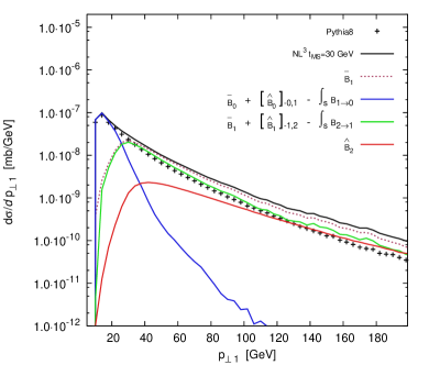
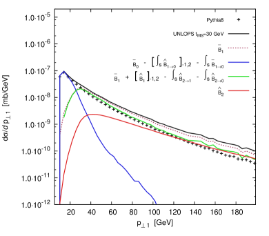
Figure 1: Transverse momentum of the hardest jet, for $\mathrm{W}$-boson production in $\mathrm{p}\mathrm{p}$ collisions at $E_{\mathrm{CM}}=7000$ GeV, when merging up to two additional partons at LO, and zero and one additional parton at NLO. Jets were defined with the $k_{\perp}$-algorithm, with $k_{\perp,min}=10$ GeV. Multi-parton interactions and hadronisation were excluded. We choose to order the contributions by the jet multiplicity in the states on which further the showering is initiated. Left panel: Results of the NL³ scheme. Right panel: Results of the UNLOPS scheme.

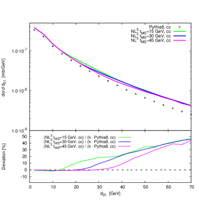
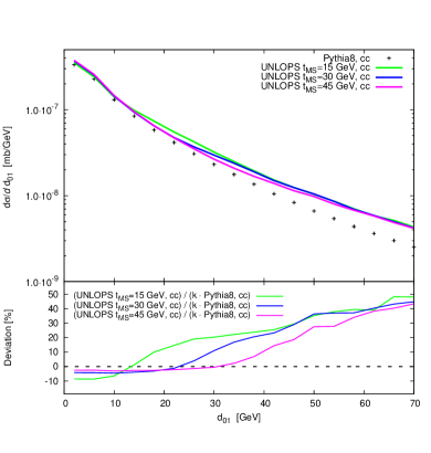
Figure 2: $k_{\perp}$- separation $d_{01}$ of the first jet and the beam, for $\mathrm{W}$-boson production in $\mathrm{p}\mathrm{p}$ collisions at $E_{\mathrm{CM}}=7000$ GeV, when merging up to two additional partons at LO, and zero and one additional parton at NLO, for three different merging scales. Jets were defined with the $k_{\perp}$-algorithm, by clustering to exactly one jet. Multi-parton interactions and hadronisation were excluded. Left panel: Results of the NL³ scheme. Right panel: Results of the UNLOPS scheme.

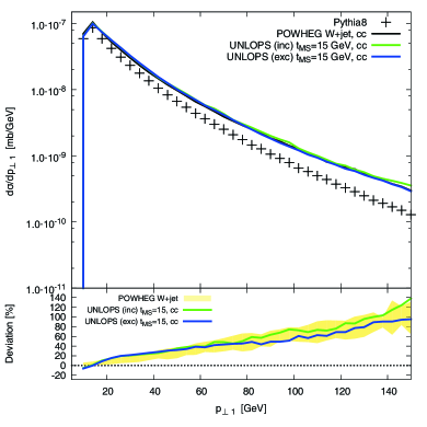
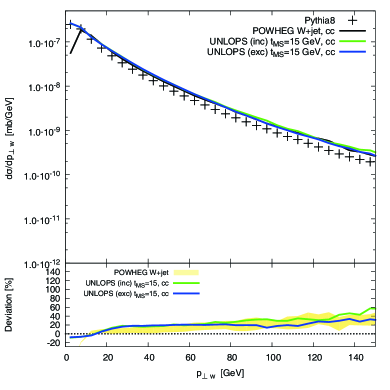
Figure 3: Comparison of using exclusive and inclusive NLO input for $\mathrm{W}$-boson production in $\mathrm{p}\mathrm{p}$ collisions at $E_{\mathrm{CM}}=7000$ GeV, when merging up to two additional partons at LO, and zero and one additional parton at NLO. Curves labelled “inc” are produced with the $\overline{\textnormal{B}}$-prescription, while “exc” indicate a generation with $\widetilde{\textnormal{B}}$-input. The lower inset shows the deviation from PYTHIA8. The band labelled “POWHEG W+jet” is given by the envelope of varying the renormalisation scale in the POWHEG-BOX program between $\frac{1}{2}\textnormal{M}_{\textnormal{\tiny{Z}}},\dots,2\textnormal{M}_{\textnormal{\tiny{Z}}}$, and the factorisation scale between $\frac{1}{2}\textnormal{M}_{\textnormal{\tiny{W}}},\dots,2\textnormal{M}_{\textnormal{\tiny{W}}}$.

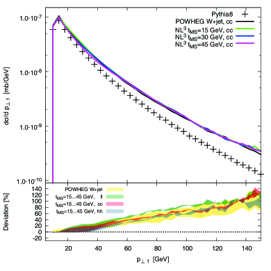
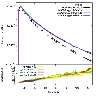
Figure 4: Transverse momentum of the hardest jet, for $\mathrm{W}$-boson production in $\mathrm{p}\mathrm{p}$ collisions at $E_{\mathrm{CM}}=7000$ GeV, when merging up to two additional partons at LO, and zero and one additional parton at NLO. Jets were defined with the $k_{\perp}$-algorithm, with $k_{\perp,min}=10$ GeV. Multi-parton interactions and hadronisation were excluded. The lower inset shows the deviation from PYTHIA8. The band labelled “POWHEG W+jet” is given by the envelope of varying the renormalisation scale in the POWHEG-BOX program between $\frac{1}{2}\textnormal{M}_{\textnormal{\tiny{Z}}},\dots,2\textnormal{M}_{\textnormal{\tiny{Z}}}$, and the factorisation scale between $\frac{1}{2}\textnormal{M}_{\textnormal{\tiny{W}}},\dots,2\textnormal{M}_{\textnormal{\tiny{W}}}$. Left panel: Results of NL³. Right panel: Results of UNLOPS.

4.1 $\mathrm{W}$-boson production

Let us start by discussing results for $\mathrm{W}$-boson production, when combining inclusive NLO calculations for $\mathrm{W}+0$- and $\mathrm{W}+1$ parton with the PYTHIA8 event generator. This section is intended mainly for validation, and we will thus switch off multi-parton interactions and hadronisation. We present results for both NL³ and UNLOPS. Our preferred method is UNLOPS, since the inclusive cross sections are there handled more consistently. By showing the results for both NL³ and UNLOPS, we hope to convey a rudimentary idea of the effect of potentially problematic logarithmic enhancements in standard observables.

Figure 1 shows the transverse momentum of the hardest jet in $\mathrm{W}$-production at the LHC, for both NL³ and UNLOPS. The sum of the solid, coloured curves gives the full NLO merged result, i.e. the black line. The dashed curve is included only to illustrate that the hard tail of the $p_{\perp 1}$-spectrum is dominated by the the $\mathrm{W}+$jet NLO sample (labelled $\bar{B}_{1}$), both in NL³ and UNLOPS, which is of course desired. This fact makes the $p_{\perp 1}$-spectra of NL³ and UNLOPS very similar.

Differences between NL³ and UNLOPS are expected in the intermediate- / low-scale regions. This is illustrated by Figure 2, which shows the $d_{01}$-distribution of the first jet. Since UNLOPS explicitly preserves the $\mathrm{W}$-production NLO cross section, the increase in the tail has to be compensated by decreasing contributions below the merging scale. The description at low $d_{01}$ in NL³ is, by construction, completely governed by the PYTHIA8 result.

Before continuing, we would again like to stress that we are using inclusive NLO cross section as input in this publication, as discussed in appendix A.2. There, it was found that making inclusive cross sections exclusive by constructing explicit phase space subtractions (through the phase space mapping of PYTHIA8) will produce slightly harder partons in the core process (see Figure 11). This tendency persists after showering, as shown in Figure 3 for the UNLOPS case. Clearly, this is a non-negligible effect, although the differences are contained in the NLO scale variation band. We believe that using exclusive input is conceptually superior. However, this section is intended to give uncertainty estimates for NLO merged parton showers, and in particular to sketch merging scale uncertainty, and there is no reason to assume that the $\overline{\textnormal{B}}$- and the $\widetilde{\textnormal{B}}$-prescription differ in this respect. Using inclusive input, however, makes merging scale variations much simpler and quicker and avoids having to tamper with the internals of the POWHEG-BOX. Because of this speed factor, we chose to use inclusive input for the results of this publication.

In the following, we will often include merging scale variations in the ratio plots. So that the plots become less cluttered, we will give the envelope of curves for merging scales between $\rho_{\textnormal{\tiny MS}}=15$ GeV and $\rho_{\textnormal{\tiny MS}}=45$ GeV as uncertainty band, rather than show the actual curves.

Figure 4 shows that the transverse momentum of the hardest jet is heavily affected by NLO merging. This is due to the $\mathrm{W}+$jet NLO calculation, as already seen in Figure 1. The merging scale variations, as well as the $\mu_{R}$/$\mu_{F}$-variation for NLO merged results lie within the scale variation band of the NLO calculation, but the combined variation is not significantly smaller. The NLO merged predictions touch the upper limit of the NLO scale variation band, because of the use of inclusive NLO input, as discussed earlier. Merging scale variations alone are minor.

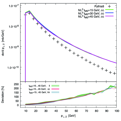
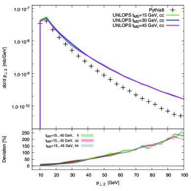
Figure 5: Transverse momentum of the second hardest jet, for $\mathrm{W}$-boson production in $\mathrm{p}\mathrm{p}$ collisions at $E_{\mathrm{CM}}=7000$ GeV, when merging up to two additional partons at LO, and zero and one additional parton at NLO. Jets were defined with the $k_{\perp}$-algorithm, with $k_{\perp,min}=10$ GeV. Multi-parton interactions and hadronisation were excluded. The lower inset shows the deviation from PYTHIA8. Left panel: Results of NL³. Right panel: Results of UNLOPS.

Merging scale uncertainties are also small in Figure 5, which shows the transverse momentum of the second hardest jet. It is particularly reassuring that even combined with $\mu_{R}$/$\mu_{F}$-variation, the bands are smaller than in CKKW-L and UMEPS [6]

We would like to conclude this section by noting that differences between UNLOPS and NL³ are hardly noticeable for the displayed observables. This is true for all observables we have investigated in $\mathrm{W}$-boson production, which can be interpreted to mean that the logarithmic improvements in UNLOPS do not result in major changes in $\mathrm{W}$-boson production for the merging scale we have chosen. We anticipate larger effects once scale hierarchies become larger, i.e.  if the merging scale is significantly decreased. For now, we will instead investigate if the introduction of a slightly larger mass scale and incoming gluons in the lowest order process leads to visible effects.

4.2 $\mathrm{H}$-boson production in gluon fusion

This section is intended to demonstrate that the PYTHIA8 implementation is not specific to $\mathrm{W}+$jets, and that different processes can be used to guide algorithmic choices. We have chosen to investigate Higgs-boson production in gluon fusion, mainly because of the presence of incoming gluons in the lowest order process and the very large NLO corrections.

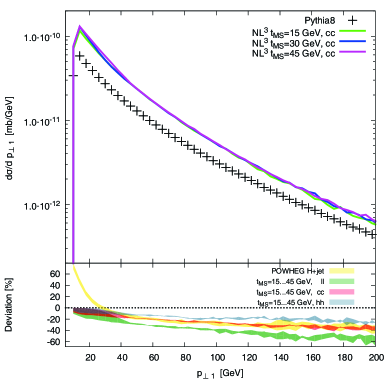
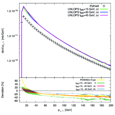
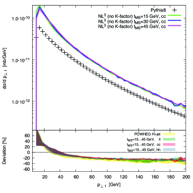
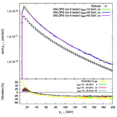
Figure 6: Transverse momentum of the hardest jet, for $\mathrm{H}$-boson production in $\mathrm{p}\mathrm{p}$ collisions at $E_{\mathrm{CM}}=7000$ GeV, when merging up to two additional partons at LO, and zero and one additional parton at NLO. Jets were defined with the $k_{\perp}$-algorithm, with $k_{\perp,min}=10$ GeV. Multi-parton interactions and hadronisation were excluded. The lower inset shows the deviation from PYTHIA8. The band labelled “POWHEG W+jet” is given by the envelope of varying the renormalisation scale in the POWHEG-BOX program between $\frac{1}{2}\textnormal{M}_{\textnormal{\tiny{Z}}},\dots,2\textnormal{M}_{\textnormal{\tiny{Z}}}$, and the factorisation scale between $\frac{1}{2}\textnormal{M}_{\textnormal{\tiny{H}}},\dots,2\textnormal{M}_{\textnormal{\tiny{H}}}$. The upper panels show the results for using the zero-jet $K$-factor (i.e. $K=\frac{\int\overline{\textnormal{B}}_{0}}{\int\textnormal{B}_{0}}$) throughout the NLO merging procedures. The lower panel show the result when not using any $K$-factor (i.e. $K=1$). Left columns: Results of NL³. Right columns: Results of UNLOPS.

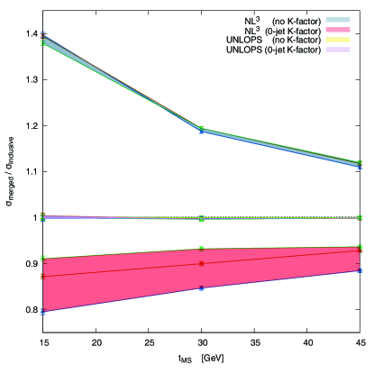
Figure 7: Comparison of inclusive cross sections for $\mathrm{H}$-production in gluon fusion $\mathrm{p}\mathrm{p}$ collisions at $E_{\mathrm{CM}}=7000$ GeV, for NL³- and UNLOPS merging, when merging up to two additional partons at LO, and zero and one additional parton at NLO. The results of the merging procedure (labelled $\sigma_{\textnormal{merged}}$) are normalised to the zero-jet inclusive NLO cross section $\sigma_{\textnormal{inclusive}}$. The coloured bands indicate the variation from choosing $\mu_{F}$ in $\left[~{}(\frac{1}{2}\textnormal{M}_{\textnormal{\tiny{H}}})^{2},\dots(2\textnormal{M}_{\textnormal{\tiny{H}}})^{2}~{}\right]$ and $\mu_{R}$ in $\left[~{}(\frac{1}{2}\textnormal{M}_{\textnormal{\tiny{Z}}})^{2},\dots(2\textnormal{M}_{\textnormal{\tiny{Z}}})^{2}~{}\right]$. The error bars represent only the statistical error on the merged cross section. The results of the NLO merging procedure are presented for two different $K$-factor treatments. The result of using no $K$-factor is labelled ”no K-factor”. Usage of the zero-jet $K$-factor is indicated by the label ”0-jet K-factor”. The same variations of NL³ and UNLOPS are plotted, although the variance in the UNLOPS results is hardly visible.

In Figure 6, we compare the variation of NLO merged results with the scale variation in the $\mathrm{H}+$jet NLO calculation of the default POWHEG-BOX program. The transverse momentum spectrum of the hardest jet is softer in NLO results than in PYTHIA8. We found the same behaviour in tree-level merging as well. Interestingly, a similar effect was observed in pure QCD dijet production, which might indicate that PYTHIA8 overestimates the hardness of radiation from initial state gluons.

We consider Figure 6 a cautionary tale. Let us examine the the upper row first. The merging scale variation in $p_{\perp 1}$ is very small. However, when including renormalisation- and factorisation-scale dependence, the uncertainty of the NLO merged results is larger than the variation in the $\mathrm{H}+$jet NLO calculation. This is explained by our choice of $K$-factor. As discussed in appendix B, this rescaling affects only the “higher orders”, since the effect on n-jet observables is removed to $\mathcal{O}\left(\alpha_{\mathrm{s}}^{n+1}\left(\mu_{R}\right)\right)$. Different choices lead to no visible effects in $\mathrm{W}$-boson production, since e.g. a change of $K_{0}=\frac{\int\overline{\textnormal{B}}_{0}}{\int\textnormal{B}_{0}}=1.16\approx 1$ will only result in changing tree-level samples slightly, and $p_{\perp 1}$ is dominated by the one-jet NLO contribution. However, this does not apply to $\mathrm{H}$ production in gluon fusion, where $K_{0}\gtrsim 2$ leads to a significantly larger two-jet tree-level contribution. Enhancing the two-jet tree-level contribution will make the leading-order scale variation of this sample more visible, thus leading to an overall larger variation.

Imposing a leading-order scale uncertainty on NLO observables is very conservative, and it seems prudent avoid artificial increases due to $K$-factors that rescale higher orders. The lower row of 6 shows the result of not using any $K$-factors at all. The agreement with POWHEG-BOX is reassuring, and the scale variation is small. The NL³ result however exhibits major merging scale variations, which are mainly induced by an increased cross section in the results for $t_{\textnormal{\tiny{MS}}}=15$ GeV. This unitarity violation was previously “masked” by a large $K$-factor.

To further illustrate the effect of including $K$-factors, we show the merged prediction of the total inclusive Higgs cross section as a function of the merging scale in Figure 7. In this figure, we divide the NLO merged results for scales $\mu_{R}$/$\mu_{F}$ by the input NLO cross section with the same $\mu_{R}$/$\mu_{F}$ choices. The ideal result should be unity, without scale uncertainties. This is true to a high degree for UNLOPS, which shows that the unitary nature of that method really works as expected. For NL³, however, we see that when using $K$-factors we get a large scale variation with a non-negligible merging scale dependence. Removing the $K$-factors decreases the scale variations, but on the other hand increases significantly the merging scale dependence.

The $K$-factor dependence is a major uncertainty in the NLO merged results for Higgs production in gluon fusion. We would like to stress that the current publication is intended as a technical summary, and not aimed at making binding predictions. Rather, we will use this as guidance when improving the implementation further.

4.3 $\mathrm{W}$-boson production compared to data

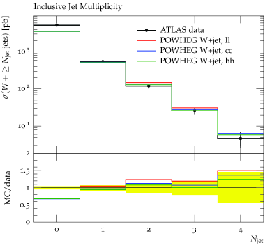
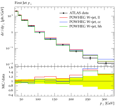
Figure 8: Jet multiplicity and transverse momentum of the hardest jet in $\mathrm{W}$-boson production, as measured by ATLAS [46]. MC results taken from the POWHEG-BOX program, with three different renormalisation/factorisation scales. Effects of partons showers, multiple scatterings and hadronisation are included.

In this section, we would like to show NLO merged predictions in comparison to data. We would like to point out that we have fixed $\alpha_{\mathrm{s}}(\textnormal{M}_{\textnormal{\tiny{Z}}})$ in the PS to $\alpha_{\mathrm{s}}(\textnormal{M}_{\textnormal{\tiny{Z}}})=0.118$, and use CTEQ6M parton distributions throughout. Please consult appendix E for a discussion of multiparton interactions. This means that the results do not correspond to a tuned version of the PYTHIA8 shower. Conclusive results can of course only be presented after the uncertainty of PS tuning has been assessed.

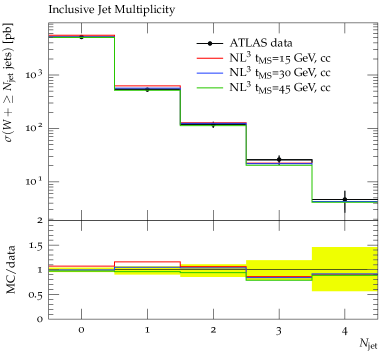
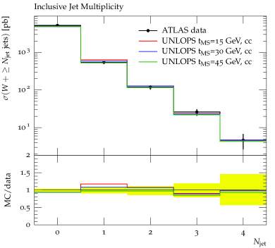
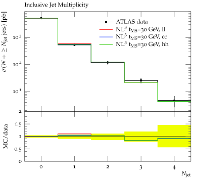
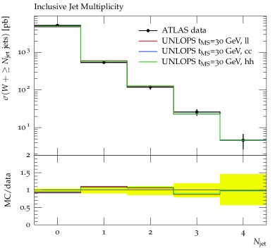
Figure 9: Jet multiplicity in $\mathrm{W}$-boson production, as measured by ATLAS [46]. The MC results were obtained by merging up to two additional partons at LO, and zero and one additional parton at NLO. MC results are shown for three different merging scales (top panels) and for three different renormalisation/factorisation scales (bottom panels). Effects of multiple scatterings and hadronisation are included. Left panels: Results of NL³. Right panels: Results of UNLOPS.

In figure 9, we show that the jet multiplicity is well under control in NLO merged predictions. The left panel of Figure 8 shows that, as expected, it is not possible to describe the number of zero-jet events with a $\mathrm{W}+$jet NLO calculation. This is of course exactly the strength of merged calculations: Observables with different jet multiplicities can be described in a single inclusive sample.

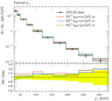
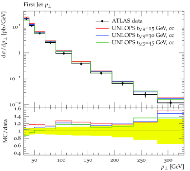
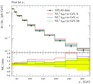
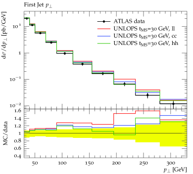
Figure 10: Transverse momentum of the hardest jet in $\mathrm{W}$-boson production, as measured by ATLAS [46]. The MC results were obtained by merging up to two additional partons at LO, and zero and one additional parton at NLO. MC results are shown for three different merging scales (top panels) and for three different renormalisation/factorisation scales (bottom panels). Effects of multiple scatterings and hadronisation are included. Left panels: Results of NL³. Right panels: Results of UNLOPS.

The transverse momentum of the hardest jet in association with a $\mathrm{W}$-boson is shown in figure 10 and the right panel of Figure 8. It is clear that the NLO merged results do not agree with data. We have chosen this particular observable because it our exhibits the most unsatisfactory description of data that we have encountered while testing our NLO merging methods. The reason for this disagreement is multifold. First, we have already mentioned that correcting for inclusive NLO input produces harder $p_{\perp 1}$ tails. The two-jet sample will eventually dominate the tail. We have chosen to rescale the two-jet contribution with a $K$-factor above unity. It could also be argued that the POWHEG-BOX result in Figure 8 has slight tendency to overshoot. This might indicate that some part of the “giant $K$-factor effect” due to enhancements of $\mathcal{O}\left(\alpha_{\mathrm{s}}\ln\frac{p_{\perp 1}^{2}}{\textnormal{M}_{\textnormal{\tiny{W}}}^{2}}\right)$ is developing in the $\mathrm{W}+$jet NLO calculation of $p_{\perp 1}$ because of soft/collinear $\mathrm{W}$-bosons. The last two points are correlated, since two-jet configurations have a major impact on the $p_{\perp 1}$-dependence of the NLO result, and increasing the two-jet contribution can enhance the visibility of giant $K$-factors.

The NL³ and UNLOPS descriptions of data exhibit high similarity. We have already noted the semblance of both methods in section 4.1. This observation is specific to $\mathrm{W}$-boson production, and does not hold for other processes, as for instance illustrated in section 4.2.

5 Discussion and conclusions

In this article, we have presented two new methods for combining multiple next-to-leading order calculations consistently with the PYTHIA8 parton shower. The NL³ method is a generalisation of the CKKW-L scheme, while the UNLOPS prescription accomplishes the same for UMEPS. Both methods achieve a description of zero-, one-, …, $n$-jet observables simultaneously at NLO accuracy in one inclusive sample, provided input event files at NLO accuracy for up to $n$ additional jets are supplied. We would like to point the interested reader to appendix D.1, in which we argue out that it is feasible to extend the UNLOPS method to a NNLO matching scheme.

Two distinct NLO merging schemes were presented to estimate the magnitude of issues related to sub-leading logarithmic enhancements. Although the UNLOPS method can be considered theoretically preferable, no large differences between NL³ and UNLOPS have been observed when merging multiple NLO calculations for $\mathrm{W}$-boson production in association with jets. This leads us to conclude that for the observables that were investigated, and the merging scale values that were used, sub-leading logarithmic enhancements are sub-dominant. For $\mathrm{H}-$boson production, differences are visible, with UNLOPS delivering a more reliable solution.

This article is intended to give a comprehensive description of the choices that can be made in deriving and implementing an NLO merging method. We hope that this publication provides enough information about the actual implementation to allow the reader to form clear judgements of the rather intricate details. We have tried to remain as general as possible in our choice of inputs. It has been shown that different inputs can, due to mismatches in phase space mappings, have visible, systematic effects. When confronted with such effects, it is clearly preferable to reach an agreement over inputs, and we hope that the current publication can contribute to a discussion.

We have shown that the merging scale dependence in $\mathrm{W}+$jets is small, and contained in the scale variation band of the $\mathrm{W}+$jet NLO calculation. This also means that the description of data is governed by the input NLO calculation.

The merging scale dependence in Higgs-boson production in gluon fusion is very small. In this case, we highlighted that the dominant uncertainty of the algorithms is given by the choice of the $K$-factor rescaling higher orders – which is beyond the control of the NLO calculation. This is a manifestation of the magnitude of $K$-factors in gluon fusion and the scale variation of the cross sections. We would like to stress that this uncertainty is present because we try to be as general as possible, and that the introduction of $K$-factors does in principle not jeopardise NLO accuracy, or degrade the PS approximation. However, if $K$-factors are not necessary and instead produce large variations, the removal of $K$-factors should be considered.

Although we have presented some comparisons to data in this article, we do not attempt to make any definite predictions. To do this, a further investigation of the uncertainties has to be performed – a task we will return to in future publications. We end this article by listing the main issues that need to be addressed.

Our methods require events generated according to the exclusive NLO cross section. There are currently no standard programs that will produce such events, and instead we have used inclusive NLO cross sections and subtracted explicit counter events by integrating tree-level matrix element events over the radiative phase space, using the mapping of the PYTHIA8 parton shower. We have also “hacked” POWHEG-BOX to directly produce the exclusive cross section event, and have found some differences, due to the different phase space mapping used there. Modifying the internals of other programs is, of course, not a viable long-term solution, and we hope that the introduction of our algorithm may inspire authors of NLO matrix element generators to include the generation of exclusive cross sections as an option in their programs.

We have allowed the use of $K$-factors in the underlying tree-level merging in the hope that the inclusion of NLO corrections will then lead to less merging scale variations. Although this can be done without modifying the formal accuracy of our methods, we see clear differences compared to the case where $K$-actors are omitted, in the case of Higgs-production, where these $K$-factors are large. We find indications of reduced factorisation and renormalisation scale uncertainties in the absence of $K$-factor, but also note larger merging scale variations in the NL³ case. This needs to be investigated further. Other options, e.g. including multiplicity-dependent $K$-factors, should also be considered to understand uncertainties.

At very high transverse momenta we expect logarithms of the form $\ln\left(\frac{p_{\perp\textnormal{jet}}}{\textnormal{M}_{\textnormal{\tiny{W}}}}\right)$ to arise, resulting in so-called “giant $K$-factors” [36, 37]. These logarithms can in principle be resummed to all orders, and an inclusion of such resummation is planned for the parton shower in PYTHIA8. We are confident that our methods can be extended also to deal with this full electro-weak shower, but meanwhile we need to understand better the uncertainties arising from these logarithms.

Finally, before we can be confident enough to make precise predictions with our new methods, a re-tuning of the shower (including MPI) of PYTHIA8 must be carried out. The currently available tunes have all been obtained without higher order matrix elements merging, and it is clear that some of the resulting parameters have been obtained from trying to fit distributions where we do not expect an uncorrected parton shower to do a reasonable job. In particular, this applies to the tuning of the scale factor in $\alpha_{\mathrm{s}}$ (see eq. (8)) in the shower, and we expect this to change significantly when tuning the ME corrected shower. This will then also directly influence the MPI, which also need to be re-tuned. Needless to say, such a tuning as a major undertaking.

Note added

While finishing this article, it came to our attention that an approach that is similar to UNLOPS has been developed in parallel by Plätzer [32]. Also, on the day of submission, we noted that Aioli et al. [47] presented their work on NLO-matching.

Appendices

Appendix A NLO prerequisites

This appendix is intended to introduce the merging scale definition used throughout this article (see section A.1), discuss the prerequisites on NLO input (section A.2), introduce the notation we employ (section A.3) and finally illustrate how the POWHEG-BOX program can be used to generate the input necessary for NLO merging (section A.4).

A.1 The Pythia jet algorithm

Throughout this paper, we use cuts on the minimal PYTHIA8 evolution $p_{\perp,evol}$, to disentangle regions of phase space. Since $p_{\perp,evol}$ defines a relative $p_{\perp}$ distance [48], we think of $p_{\perp,evol}$ as an inter-parton separation criterion. To avoid confusion with other $p_{\perp}-$definitions, we will use the symbol $\rho$ for $p_{\perp,evol}$.

The phase space regions in which we believe fixed-order calculations to dominate is separated from the resummation region by a cut value $\rho_{\textnormal{\tiny MS}}$, defined in a parton separation $t\sim\min\{\rho\}$. This minimal separation is constructed by finding the minimal $\rho$ for any triplet of partons $e,r,s$, where $e$ is a final state “emitted” parton, $r$ is a radiating parton and $s$ is a spectator. All triplets, irrespectively of flavour (or colour) constraints are included. In a dipole picture, the radiator $r$ can be thought of as the dipole end whose momentum changes most when splitting the dipole $(r^{\prime},s^{\prime})$ into two dipoles $(r,e),~{}(e,s)$ while $s$ is the dipole end that absorbs the (small) recoil. The functional definition of this parton separation criterion is

$$t~{}=~{}\min\left[\rho_{\{i,j,k\}}\right]\qquad\textnormal{where $i\in$ \{final state partons\},}$$ (36)

and $$j\in$$ {final and initial state partons},

and $$k\in$$ {final and initial state partons}

where the separation of $i$ for a fixed triplet $(i,j,k)$ of partons with momenta $p_{i},p_{j},p_{k}$ is

$$\rho_{ijk}~{}=~{}p^{2}_{\perp,evol,ijk}~{}=~{}\begin{cases}z_{ijk}(1-z_{ijk})Q_{ij}^{2}&\textnormal{if the radiator $j$ is a final state parton, and}\\ &Q_{ij}^{2}=(p_{i}+p_{j})^{2}~{},\quad z_{ijk}=\frac{x_{i,jk}}{x_{i,jk}+x_{j,ik}}\\ &x_{i,jk}=\frac{2p_{i}(p_{i}+p_{j}+p_{k})}{(p_{i}+p_{j}+p_{k})^{2}}\\ (1-z_{ijk})Q_{ij}^{2}&\textnormal{if the radiator $j$ is an initial state parton, and}\\ &Q_{ij}^{2}=-(p_{i}-p_{j})^{2}~{},\quad z_{ijk}=\frac{(p_{i}-p_{j}+p_{k})^{2}}{(p_{i}+p_{k})^{2}}\\ \end{cases}$$ (37)

The cut value $\rho_{\textnormal{\tiny MS}}$ is called merging scale. If all $\rho_{ijk}$ for a particular final state parton $i$ are larger than $\rho_{\textnormal{\tiny MS}}$, we call this parton a resolved jet. Conversely, if any $\rho_{ijk}$ is below $\rho_{\textnormal{\tiny MS}}$, we call $i$ an unresolved jet. We say that a phase space point is in the matrix element region if $t>\rho_{\textnormal{\tiny MS}}$, i.e. all minimal parton separations are larger than the cut. In other words, a phase space point is in the matrix element region if it only contains resolved jets. The parton shower region is disjoint: If any jet separation falls below $\rho_{\textnormal{\tiny MS}}$, be believe that parton shower resummation is appropriate.

Using eq. (36) and eq. (37) as merging scale definition does not exactly correspond to separating the matrix element- and parton shower regions in $p_{\perp,evol}$. In parton shower algorithms, the resolution scale attributed to a state is given by the scale of the last splitting. This is just one number, since a splitting is generated by a winner-takes-it all strategy: If a splitting is chosen, all scales attributed to splittings of other partons are considered higher. Such a merging scale definition can only be constructed if we know (all) parton shower histories of an input event.

For now, we use eq. (36) and eq. (37) as merging scale definitions, and are content with the fact that $\rho_{\textnormal{\tiny MS}}$ does still correspond to a single $p_{\perp,evol}-$value. This means that vetoing shower emissions that would result in an additional resolved jet will not introduce no-emission probabilities above $\rho_{\textnormal{\tiny MS}}$.

We have to point out that fixing the merging scale definition is necessary in the NLO merging methods illustrated in this article. Otherwise, it would be mandatory to reweight NLO corrections with no-emission probabilities for merging-scale-unordered emissions, which would fundamentally degrade the higher-order description we aim to achieve. One benefit of CKKW-L tree-level merging is that the method allows for a wide class of merging scale definitions. Because of the treatment of emissions that are unordered in the merging scale, however, the merging scale effectively has to define a hardness-measure, since otherwise, only small portions of phase space will be endowed with ME corrections [5]. Different choices of hardness definitions for different processes in CKKW-L can be helpful for efficiently correcting phase space. The current implementation of CKKW-L in PYTHIA8 allows for both $\min\{\rho\}$ and $\min\{k_{\perp}\}$ as merging scales. No major efficacy differences between these merging scale definitions has been found so far, leading us to conclude that in practise, defining the merging scale in $\min\{\rho\}$ is reasonable.

A.2 Exclusive cross sections

In this section, we would like to introduce the concepts of exclusive and inclusive NLO cross sections, and comment on how inclusive NLO cross sections can be made exclusive by the inclusion of a phase space subtraction sample.

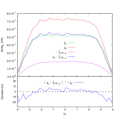
Figure 11: Comparisons of two way of generating exclusive NLO cross sections. $\overline{\textnormal{B}}_{i}$ events are calculated without changing the POWHEG-BOX program, while for $\widetilde{\textnormal{B}}_{i}$, we have explicitly introduced the necessary cuts in POWHEG-BOX. Left panel: Comparison for zero-jet exclusive NLO cross section, as function of the $\mathrm{W}$-boson rapidity. Right panel: Comparison for one-jet exclusive NLO cross section, as function the kinematical transverse momentum of the parton.

We think of matrix element merging as a two-step measurement. We first measure the number of resolved jets in the input event, by applying a cut. Then, we calculate an interesting observable on events that have been classified as $n-$jet events. To make the second step independent of the choices in the first measurement, we need to sum over all possible jet multiplicities.

Throughout this publication, we will define jets by the PYTHIA8 evolution $p_{\perp}$ jet separation criterion, as discussed in appendix A.1. Resolved jets are defined as partons whose separation to any other partons in the state is above the value $\rho_{\textnormal{\tiny MS}}$. We call $\rho_{\textnormal{\tiny MS}}$ the merging scale.

The output of a tree-level calculations for $k$ final partons can contain $l=0,\dots,k$ partons with soft or collinear momenta. The result of the calculation will diverge as soon as any parton in the calculation becomes soft or collinear. We can remove these regions of phase space, if we enforce that the output only contains exactly $k$ partons with jet separation above $\rho_{\textnormal{\tiny MS}}$, i.e. $k$ resolved jets. If the jet definition is infrared and collinear safe, this jet cut will render tree-level calculations finite.

The result of using a next-to-leading order calculation for $k$ partons to describe an observable $\mathcal{O}$ can schematically be written as

$$\!\!\!\langle\mathcal{O}\rangle = \int d^{k}\phi~{}\mathcal{O}(\phi_{k})~{}d\sigma_{Born}+\int d^{k}\phi~{}\mathcal{O}(\phi_{k})~{}d\sigma_{Virtual}+\int d^{k+1}\phi~{}\mathcal{O}(\phi_{k+1})~{}d\sigma_{Real}~{},\qquad$$ (38)

where $\int d^{k}\phi$ indicates an integration over the $k-$parton phase space, $d\sigma_{Born}$ is the tree-level cross section, $d\sigma_{Virtual}$ the virtual correction term and $d\sigma_{Real}$ the real emission part. Equation 38 allows contributions of any number of $l=0,\dots,k+1$ resolved (or unresolved) jets. Since the tree-level part still diverges if any of the $k$ partons approach the soft and collinear regions, we require that $\int_{k}\mathcal{O}(\phi_{k})d\sigma_{Born}$ always contains exactly $k$ resolved jets, which immediately means having the same requirement in $\int_{k}\mathcal{O}(\phi_{k})d\sigma_{Virtual}$. This then means that $\int_{k+1}\mathcal{O}(\phi_{k+1})d\sigma_{Real}$ has to be constrained, since otherwise, the NLO calculation could include real-emission corrections to non-existent “underlying” Born configurations with less than $k$ resolved jets. The POWHEG method [17, 18] eliminates this issue by evaluating using one phase space point $\overline{\phi}_{n}$ for tree-level and virtual parts, and $\phi_{n+1}$ phase space points that can be projected exactly onto $\overline{\phi}_{n}$ in real-emission terms. We will assume that in neither of the terms in 38, less than $k$ resolved jets are included. Further, the observable $\mathcal{O}$ receives – through real corrections – contributions from $k+1$ (resolved or unresolved) jets. Measurements explicitly depending on the kinematics of $k+1$ resolved jets are only accurate to tree-level approximation, while contributions for an unresolved additional jet are necessary to cancel divergences

In multi-jet merging, $(k+1)-$jet contributions enter through explicitly adding a reweighted $(k+1)-$jet sample. To merge multiple NLO calculations, we also need a clean cut, that makes the classification of the input in terms of jet multiplicities possible. We define that the “NLO part” of an $k-$jet NLO calculation should contain $k$ resolved jets, and at most one unresolved jet, while contributions with $k+1$ resolved jets are regarded leading-order parts

$$\langle\mathcal{O}\rangle = \underbrace{\int d^{k}\phi~{}\mathcal{O}(\phi_{k})~{}\left\{~{}d\sigma_{Born}~{}+~{}d\sigma_{Virtual}~{}+~{}\int^{\rho_{\textnormal{\tiny MS}}}d\phi~{}d\sigma_{Real}\right\}}_{\textnormal{NLO part}}$$

$$+\underbrace{\int_{\rho_{\textnormal{\tiny MS}}}d^{k+1}\phi~{}\mathcal{O}(\phi_{k+1})~{}d\sigma_{Real}}_{\textnormal{LO part}}$$

We call the NLO part of such a calculation the exclusive NLO cross section.

Merging schemes naturally act on exclusive cross sections. Technically, we assume that all unresolved real emission parts are projected onto $n$-parton phase space points. In POWHEG, this is facilitated by performing the $d\phi$ integration in the real-emission term explicitly. If an NLO calculation would yield only phase space points with exactly $n$ partons in $n$ resolved jets, and weight these points with

$$\widetilde{\textnormal{B}}_{n}=d\sigma_{Born}~{}+~{}d\sigma_{Virtual}~{}+~{}\int^{\rho_{\textnormal{\tiny MS}}}d\phi~{}d\sigma_{Real}~{},$$ (40)

then this calculation could be used immediately for NLO merging. However, $\widetilde{\textnormal{B}}_{n}$ might not be accessible without changing the NLO matrix element generator, since it might not possible to split the calculation into “NLO parts” and “LO parts” as desired. We instead choose to write

$$\widetilde{\textnormal{B}}_{n}=d\sigma_{Born}~{}+~{}d\sigma_{Virtual}~{}+~{}\int d\phi~{}d\sigma_{Real}~{}-~{}\int_{\rho_{\textnormal{\tiny MS}}}d\phi~{}d\sigma_{Real}$$ (41)

and to use the two samples

$$\overline{\textnormal{B}}_{n} = ~{}d\sigma_{Born}~{}+~{}d\sigma_{Virtual}~{}+~{}\int d\phi~{}d\sigma_{Real}$$ (42)

$$-\int_{s}\textnormal{B}_{n+1\rightarrow n} = ~{}-~{}\int_{\rho_{\textnormal{\tiny MS}}}d\phi~{}d\sigma_{Real}$$ (43)

separately. We call $\overline{\textnormal{B}}_{n}$ the inclusive NLO cross section, and refer to $\int_{s}\textnormal{B}_{n+1\rightarrow n}$ as phase space subtraction term. Adding the inclusive NLO cross section and the subtraction term, we retrieve the exclusive NLO cross section. It is possible to formulate NLO merging acting on exclusive cross sections, or acting on inclusive cross sections and additional phase space subtraction samples.

We would like to comment on our framework to generate exclusive cross sections from inclusive NLO input. It has already been demonstrated in [6] that extracting integrated states that had been constructed as intermediate states in the parton shower history does indeed give the expected results (see Figure 2 of [6]). However, these comparisons were performed between the shower approximation and the integrated matrix element. To correct for the use of an inclusive NLO cross section, we have to use integrated tree-level events as phase space subtraction for POWHEG-BOX events. Figure 11 shows how the exclusive cross section generated through explicitly changing the POWHEG-BOX program code compares to the exclusive cross section produced by a-posteriori phase space subtraction. The differences between the two prescriptions stems from a different phase space mapping in POWHEG-BOX and PYTHIA8. Such effects are beyond the accuracy of the NLO merging methods presented in this article. It should be noted that an a-posteriori phase space subtraction using the PYTHIA8 phase space mapping produces a harder $p_{\perp}$-spectrum and less forward $\mathrm{W}$-bosons. Ideally, we would like generate the exclusive NLO cross section with an NLO generator which allows for the necessary cuts, so that explicit phase space subtraction become unnecessary. For this publication however, we will use subtractions, since this allows us to perform merging scale variations without continuously having to re-generate LHEF output with the POWHEG-BOX program.

A.3 Notation

Formulating NLO merging is unfortunately a fairly notation-heavy task. In this section, we would like to carefully introduce the symbols we will use throughout this article in a tabular style, for easy reference. Let us define the lingo

$\phi_{n}$:	Phase space point with $n$ additional resolved jets. This means that $\phi_{n}$ can contain $p$ lowest-multiplicity particles (e.g. $\mathrm{e}^{+}$ and $\mathrm{e}^{-}$ for Drell-Yan production), and $n$ additional partons. Each phase space point has a fixed momentum, flavour and colour configuration.
Underlying configuration:	Phase space point $\phi_{n}$ which can be to constructed from $\phi_{n+1}$ by removing one emission, meaning integrating over the one-particle phase space of the emission, and recombining flavours and colours. We will use the terms underlying momentum configuration, underlying flavour configuration and underlying colour configuration when explicitly emphasising one aspect of the underlying configuration.
$\Phi_{\textnormal{rad}}:$	The radiative phase space, meaning that in $\displaystyle\phi_{n+1}\approx\phi_{n}\Phi_{\textnormal{rad}}$ (44) $\Phi_{\textnormal{rad}}$ plays the role of the one-particle phase space of the additional parton, while $\phi_{n}$ is the underlying configuration.
Resolved jet:	Parton, for which all possible jet separations to other partons in this phase space point are larger than the value $\rho_{\textnormal{\tiny MS}}$.
Unresolved jet:	Parton, for which at least one jet separations to one other partons in this phase space point is lower than the value $\rho_{\textnormal{\tiny MS}}$.

We always assume that matrix elements for $n$ outgoing partons are only integrated over phase space regions with exactly $n$ resolved jets, unless explicitly stated otherwise. In cases where we integrate over emissions, we assume that in the ME input, all partons were resolved jets, and that after the integration, all partons are resolved jets.

Please note that the methods presented in this publication do not rely on a particular regularisation scheme in the NLO calculation, as long as the dependence on the regularisation scheme is cancelled locally, i.e. in the weight of each phase space points separately. We will choose a rather symbolic notation for parts of NLO calculations, and hope that this will make the formulae in this article more accessible. In the following, we would like to introduce the shorthands:

$\textnormal{B}_{n}$:	Tree-level matrix element with $n$ partons, i.e.   $\displaystyle\textnormal{B}_{n}$ $\displaystyle=$ $\displaystyle f_{n}^{+}(x_{n}^{+},\mu_{F})f_{n}^{-}(x_{n}^{-},\mu_{F})\left|\mathcal{M}_{n,0}\left(\mu_{F},\mu_{R}\right)\right|^{2}~{},$ (45) where the first subscript on $\left|\mathcal{M}_{n,0}\left(\mu_{F},\mu_{R}\right)\right|^{2}$ indicates the number of jets, while the second counts loop integrations. Readers more familiar with the notation of [18] should note $\displaystyle\textnormal{B}_{n}$ $\displaystyle=$ $\displaystyle\left[~{}B(\Phi_{n})~{}\right]_{f_{b}}$ For brevity, we always suppress flavour indication on $\textnormal{B}_{n}$.
$\textnormal{B}_{n+1|n}$:	Sum of tree-level configurations with $n+1$ partons, for which the underlying Born configuration is $\phi_{n}$. Loosely, we think of $\textnormal{B}_{n+1|n}$ as the sum of matrix elements $\textnormal{B}_{n}$, multiplied by splitting kernels (with $\textnormal{B}_{n}$ being evaluated using the underlying momentum, flavour and colour configuration, while the splitting kernels depend on the radiative phase space). Translating to the notation of [18], this means $\displaystyle\int d\Phi_{\textnormal{rad}}\textnormal{B}_{n+1|n}~{}=~{}\sum_{\alpha_{r}\in\{\alpha_{r}|f_{b}\}}~{}\int~{}\left[~{}d\Phi_{rad}~{}R(\Phi_{n+1})~{}\right]^{\overline{\Phi}^{\alpha_{r}}_{n}=\Phi_{n}}_{\alpha_{r}}$ We choose the more symbolic indexing with $n+1|n$, rather than the more rigorous $\alpha_{r}$-notation of [18], in order to not obfuscate formulae with details that are not essential for the discussion.
$\int_{s}\textnormal{B}_{n\rightarrow m}$:	Sum of tree-level cross sections with $n$ resolved jets in the input ME events, after integration over the phase space of $n-m$ partons. Symbolically: $\displaystyle\int_{s}\textnormal{B}_{n\rightarrow m}~{}=~{}\sum_{n}\int_{s}d^{n-m}\phi~{}\textnormal{B}_{n|n-m}$ (46) We think of $\phi_{n}$ being produced from $\phi_{n-m}$ by $m$ consecutive splittings. The index $s$ denotes that the integration is accomplished by explicitly removing $m$ partons from the $n-$parton phase space, meaning that we substitute the state $S_{+n}$ by the state $S_{+n-m}$, as introduced in [6]. The symbol $\int_{s}\textnormal{B}_{n\rightarrow m}$ also indicates that the state $S_{+m}$ only has resolved jets, and that possibly more than one integrations had to be performed in case all of the states $S_{+n-1},\dots,S_{+m+1}$ contained unresolved jets.
$\int_{s}\textnormal{B}_{n\rightarrow m}^{\uparrow}$:	Sum of tree-level cross sections with $n$ resolved jets in the input ME events, after integration over the phase space of $n-m$ partons. However, in contrast to the symbol $\int_{s}\textnormal{B}_{n\rightarrow m}$, we explicitly require the states $S_{+n-1}$ to contain $n-1$ resolved jets, and still perform this second integration. This is indicated by the upward-pointing arrow. All further integrations only have to be performed because the states $S_{+n-2},\dots,S_{+m+1}$ contained unresolved jets. $\int_{s}\textnormal{B}_{3\rightarrow 0}^{\uparrow}$ for example means that we first replace the state $S_{+3}$ by $S_{+2}$ (with two resolved jets), then demand another integration, giving $S_{+1}$. Then, we find that $S_{+1}$ contains an unresolved jet, so that we integrate once more. The last step would not be necessary for the term $\int_{s}\textnormal{B}_{3\rightarrow 1}^{\uparrow}$.
$\textnormal{V}_{n}$:	Virtual correction matrix element with $n$ partons above $\rho_{\textnormal{\tiny MS}}$: $\displaystyle\textnormal{V}_{n}$ $\displaystyle=$ $\displaystyle f_{n}^{+}(x_{n}^{+},\mu_{F})f_{n}^{-}(x_{n}^{-},\mu_{F})\left|\mathcal{M}_{n,1}\left(\mu_{F},\mu_{R}\right)\right|^{2}~{},$ (47) We assume that all ultraviolet divergences have already been removed.
$\textnormal{D}_{n+1|n}$:	Sum of infrared regularisation terms with $n$ partons above $\rho_{\textnormal{\tiny MS}}$. As above, we indicate these terms can be projected onto underlying Born configurations by the index $n+1|n$. For simplicity, we may think of these regulators as Catani-Seymour dipoles, and very symbolically put $\displaystyle\textnormal{D}_{n+1|n}$ $\displaystyle\sim$ $\displaystyle\sum_{i^{\prime}j^{\prime}k}f_{n}^{+}(x_{n}^{+},\mu_{F})f_{n}^{-}(x_{n}^{-},\mu_{F})\left|\mathcal{M}_{n,0}\left(\mu_{F},\mu_{R},\bar{\phi_{n}}\right)\right|^{2}$ $\displaystyle\qquad\qquad\otimes~{}D_{ij\rightarrow i^{\prime}j^{\prime}k}\left(\Phi_{\textnormal{rad}}\right)~{},$ where $i$ and $j$ are partons of the underlying configuration $\bar{\phi_{n}}$, while $i^{\prime},j^{\prime}$ and $k$ are partons of $\phi_{n+1}$. As long as all dependence on the regularisation is contained in the inclusive (exclusive) NLO cross sections, our method will not depend on the actual form of these terms – all numerical NLO subtraction schemes are equally valid. The notation $n+1|n$ is to be understood in the same way as for $\textnormal{B}_{n+1|n}$.
$\textnormal{I}_{n+1|n}$:	Sum of integrated infrared regularisation terms with $n$ partons above $\rho_{\textnormal{\tiny MS}}$. Remainders due to initial state partons being collinear with identified initial hadrons are included in $\textnormal{I}_{n+1|n}$. As above, we indicate that the terms in $\textnormal{I}_{n+1|n}$ can be projected unto underlying configurations by the index $n+1|n$. Schematically $\displaystyle\textnormal{I}_{n+1|n}$ $\displaystyle\sim$ $\displaystyle\int d\Phi_{\textnormal{rad}}\textnormal{D}_{n+1|n}$ (49) In this case, the one-parton phase space integration is commonly performed analytically. The integration here covers the complete radiative phase space. Integration variables can change for different types of dipoles $D_{ij\rightarrow i^{\prime}j^{\prime}k}$.
$\overline{\textnormal{B}}_{n}$:	Inclusive NLO weight of $n-$parton phase space points. $\displaystyle\overline{\textnormal{B}}_{n}$ $\displaystyle=$ $\displaystyle\textnormal{B}_{n}+\textnormal{V}_{n}+\textnormal{I}_{n+1|n}$ (50) $\displaystyle+\int d\Phi_{\textnormal{rad}}\left(\textnormal{B}_{n+1|n}-\textnormal{D}_{n+1|n}\right)~{}.$ Note that we will assume that this gives a NLO weight for the phase space point $\phi_{n}$, meaning that we have to evaluate $\textnormal{D}_{n+1|n}$ and $\textnormal{I}_{n+1|n}$ with $\phi_{n}$ rather than $\bar{\phi_{n}}$. This is the standard procedure in the POWHEG and MC@NLO methods. The integration over $\Phi_{\textnormal{rad}}$ covers the full radiative phase space. Real emission terms can give contributions with an additional resolved jet, which are here included into the weight of $n$-jet phase space points $\phi_{n}$. As discussed above, the description of an observable at NLO receives $n$-jet and a $n+1$-jet contributions, so that projecting all $n+1$-jet configurations onto $\phi_{n}$ (and leaving no $n+1$ events) seems problematic. However, in matrix-element merging, $n+1$-jet events will be included though the next-higher multiplicity sample. We then need to ensure that the contribution of resolved $n+1$-jet events to the cross section is not double-counted. This is solved by the introduction of exclusive NLO jet cross sections. The inclusive cross section is closely related to the definition of $\bar{B}$ in the POWHEG method. Indeed, if no Sudakov factors are applied in the weight of Born-type phase space points in POWHEG, and all radiative events are projected unto Born configurations, this exactly produces our definition of $\overline{\textnormal{B}}_{n}$.
$\widetilde{\textnormal{B}}_{n}$:	Exclusive NLO weight of $n-$parton phase space points, $\displaystyle\widetilde{\textnormal{B}}_{n}$ $\displaystyle=$ $\displaystyle\textnormal{B}_{n}+\textnormal{V}_{n}+\textnormal{I}_{n+1|n}$ (51) $\displaystyle+\int^{\rho_{\textnormal{\tiny MS}}}\!\!\!\!d\Phi_{\textnormal{rad}}\left(\textnormal{B}_{n+1|n}-\textnormal{D}_{n+1|n}\right)$ $\displaystyle=$ $\displaystyle\overline{\textnormal{B}}_{n}-\int_{\rho_{\textnormal{\tiny MS}}}d\Phi_{\textnormal{rad}}\textnormal{B}_{n+1|n}$ $\displaystyle=$ $\displaystyle\overline{\textnormal{B}}_{n}-\int_{s}\textnormal{B}_{n+1\rightarrow n}~{}.$ It is clear from the last equality that an exclusive NLO $n-$jet cross section can be constructed from the inclusive case by explicitly subtracting the phase space points with an additional resolved jet.
$\int_{s}\overline{\textnormal{B}}_{n\rightarrow m}$:	Inclusive NLO cross section with $n$ resolved jets in the input ME events, after integration over the phase space of $n-m$ partons. The symbol $\int_{s}\overline{\textnormal{B}}_{n\rightarrow m}$ as always also indicates that more than one integrations had to be performed because all of the states $S_{+n-1},\dots,S_{+m+1}$ contained unresolved jets.
$\int_{s}\widetilde{\textnormal{B}}_{n\rightarrow m}$:	Exclusive NLO cross sections with $n$ resolved jets in the input ME events, after integration over the phase space of $n-m$ partons. The symbol $\int_{s}\widetilde{\textnormal{B}}_{n\rightarrow m}$ as always also indicates that more than one integrations had to be performed because all of the states $S_{+n-1},\dots,S_{+m+1}$ contained unresolved jets.

We will use several different event samples as input for multi-jet merging. An event consists of a phase space point with an associated weight, and can thus be considered completely differential. Only if necessary will we talk about predictions for an observable. We will use “cross section” and “event” interchangeably, and also make little distinction between the terms “(phase space) weight” and “matrix element”.

Exclusive cross sections are the basic building blocks needed for multi-jet merging. Tree-level merging uses phase space points weighted with exclusive tree-level matrix elements $\textnormal{B}_{n}$ as input. The NLO multi-jet merging prescriptions advocated in this publication analogously require phase space points weighted by exclusive NLO weights as input. If no exclusive calculation is available, it is possible to extend the algorithm to include the explicit subtraction of eq. (LABEL:eq:btilde-explicit). To make formulae for NLO merging a bit more transparent, let us introduce the short-hands

$\widehat{\textnormal{B}}_{n}$:	UMEPS-reweighted tree-level cross sections with $n$ resolved jets in the input ME events.
$\int_{s}\widehat{\textnormal{B}}_{n\rightarrow m}$:	UMEPS-reweighted tree-level cross sections with $n$ resolved jets in the input ME events, after integration over the phase space of $n-m$ partons. The symbol $\int_{s}\widehat{\textnormal{B}}_{n\rightarrow m}$ also indicates that more than one integrations had to be performed because all of the states $S_{+n-1},\dots,S_{+m+1}$ contained unresolved jets.
$\left[\vphantom{\sum}A\right]_{-a,b}$:	Contribution $A$, with terms of powers $\alpha_{\mathrm{s}}^{a}$ and $\alpha_{\mathrm{s}}^{b}$ removed. The resulting terms are calculated with fixed scales $\mu_{R}$ and $\mu_{F}$.
$\left[\vphantom{\sum}A\right]_{c,d}$:	Contribution $A$, with only terms of power $\alpha_{\mathrm{s}}^{c}$ and $\alpha_{\mathrm{s}}^{d}$ retained, calculated with fixed scales $\mu_{R}$ and $\mu_{F}$.

The last two short-hands are particularly useful when trying to summarise terms in the expansion of the tree-level merging weights. For example, the sum of the second and third term in curly brackets in

$$\left[\vphantom{\sum}\textnormal{B}_{2}w_{2}\right]_{-2,3} = \textnormal{B}_{2}\left\{w_{2}^{\prime}-\left[\vphantom{\sum}w_{2}^{\prime}\right]_{0}-\left[\vphantom{\sum}w_{2}^{\prime}\right]_{1}\right\}$$

is given by eq. (109) below.

A.4 Powheg-Box usage

This section is intended to give guidelines on how to use the POWHEG-BOX program [19] in order to produce the inclusive NLO cross sections [41, 43, 42, 44] needed for NLO merging in PYTHIA8. Ideally, this should suffice as tutorial on how to set up the desired POWHEG-BOX outputs. We rely on knowledge on POWHEG-BOX input manipulations. With new versions of POWHEG-BOX, the names of the inputs might change, so that the settings advocated here come without guarantees.

For a given process with $n$ partons in the underlying Born configuration, POWHEG-BOX by default generates output Les Houches events with $n-$ and $(n+1)-$parton kinematics. $n-$parton phase space points are weighted with the matrix element weights

$$\overline{\textnormal{B}}_{n}~{}\Delta\left(p_{\perp,min}\right)$$ (53)

$$= \Bigg{\{}\textnormal{B}_{n}\left(\phi_{n}\right)+\textnormal{V}_{n}\left(\phi_{n}\right)+\textnormal{I}_{n+1|n}\left(\phi_{n}\right)$$

$$\qquad+\int\!\!d\Phi_{\textnormal{rad}}\left[\textnormal{B}_{n+1|n}\left(\phi_{n}\,\phi_{rad}\right)-\textnormal{D}_{n+1|n}\left(\phi_{n}\,\phi_{rad}\right)\right]\Bigg{\}}~{}\Delta\left(p_{\perp,min}\right)~{},$$

where the integration $\int d\Phi_{\textnormal{rad}}$ contains the complete radiative phase space, and the Sudakov factor is given by

$$\Delta\left(p_{\perp}\right) = \exp\left\{-\int_{p_{\perp}}\!\!d\Phi_{\textnormal{rad}}^{\prime}\frac{\textnormal{B}_{n+1|n}\left(\phi_{n},\phi_{rad}^{\prime}\right)}{\textnormal{B}_{n}\left(\phi_{n}\right)}\right\}~{}.$$ (54)

$(n+1)-$parton phase space points are weighted with

$$\overline{\textnormal{B}}_{n}~{}\Delta\left(p_{\perp}\right)~{}\frac{\textnormal{B}_{n+1|n}\left(\phi_{n+1}\right)}{\textnormal{B}_{n}\left(\phi_{n}\right)}\Theta\left(p_{\perp}-p_{\perp,min}\right).$$ (55)

The program decides if a radiative (i.e. $(n+1)-$parton) phase space point is generated by comparing the $p_{\perp}$ of the proposed configuration $\phi_{n+1}$ against $p_{\perp,min}$. No radiative events are produced if $p_{\perp,min}$ is set to the kinematical limit. Furthermore, we have

$$\left\{\Delta\left(p_{\perp,min}\right)\right\}_{p_{\perp,min}\rightarrow\infty}=1~{}.$$ (56)

Thus, using $p_{\perp,min}\rightarrow\infty$, we find

$$\left\{\overline{\textnormal{B}}_{n}~{}\Delta\left(p_{\perp,min}\right)\right\}_{p_{\perp,min}\rightarrow\infty} = \textnormal{B}_{n}\left(\phi_{n}\right)+\textnormal{V}_{n}\left(\phi_{n}\right)+\textnormal{I}_{n+1|n}\left(\phi_{n}\right)$$

$$\qquad+\int\!\!d\Phi_{\textnormal{rad}}\left[\textnormal{B}_{n+1|n}\left(\phi_{n}\,\phi_{rad}\right)-\textnormal{D}_{n+1|n}\left(\phi_{n}\,\phi_{rad}\right)\right]$$

This is exactly the inclusive NLO cross section we need to perform NLO merging. The NLO merging prescription will include $(n+1)-$parton configurations in a CKKW-L style.

In the POWHEG-BOX program, the parameter $p_{\perp,min}$ can be set by changing the input variable ptsqmin. For example assigning

$${\tt ptsqmin=1d15}$$ (58)

will ensure that for LHC energies, the output events of POWHEG-BOX will contain only $n-$parton kinematics, weighted with the desired inclusive NLO cross section. Setting ptsqmin will produce only $n-$parton kinematics only if every $(n+1)-$parton phase space has an underlying Born configuration. This is for example not true for $\mathrm{c}\bar{\mathrm{c}}\to\mathrm{u}\bar{\mathrm{d}}\mathrm{W}^{-}$ scattering via an $s-$channel gluon. Since such processes do not constitute corrections to any lower-order process, we regard these as true leading-order parts, and (internally) neglect these configuration in the POWHEG-BOX output. They will be added by including such configurations with incomplete parton shower histories through the treatment of tree-level matrix elements. Numerically, the treatment of incomplete states does not have any impact.

The desired POWHEG-BOX output should be generated with fixed factorisation- and renormalisation scale. To be completely certain that this is the case, set

$${\tt runningscale\quad 0}$$ (59)

$${\tt runningscales\quad 0}$$ (60)

$${\tt btlscalereal\quad 1}$$ (61)

$${\tt btlscalect\quad 1}$$ (62)

$${\tt ckkwscalup\quad 0}$$ (63)

The POWHEG-BOX program would, upon making the assignment 58, attribute a SCALUP value of ${\tt SCALUP}=\sqrt{{\tt ptsqmin}}$ to the output LH events. This number would normally be read by PYTHIA8 and used as factorisation scale in the construction of overestimates for initial state splittings. For our purposes, the true value of $\mu_{F}$ will be an input for PYTHIA8, so that the correct choice can be used internally.

After these settings, the POWHEG-BOX output file can be used for NLO merging in PYTHIA8. We will include a detailed documentation of this procedure, and a manual how the schemes presented in this publication can be used, in the online documentation of an upcoming PYTHIA8 release.

Appendix B Generation of weights

The aim of this appendix is to provide a complete description of the $\mathcal{O}\left(\alpha_{\mathrm{s}}^{1}\left(\mu_{R}\right)\right)-$terms needed to implement the NL³ and UNLOPS schemes. This task is split into subsections containing the expansion of factors appearing in the weight $w_{n}$

$$w_{n} = K\cdot\tfrac{x_{n}^{+}f_{n}^{+}(x_{n}^{+},\rho_{n})}{x_{n}^{+}f_{n}^{+}(x_{n}^{+},\mu_{F})}\tfrac{x_{n}^{-}f_{n}^{-}(x_{n}^{-},\rho_{n})}{x_{n}^{-}f_{n}^{-}(x_{n}^{-},\mu_{F})}\prod_{i=1}^{n}\Bigg{[}\frac{\alpha_{\mathrm{s}}(b_{i}\rho_{i})}{\alpha_{\mathrm{s}}(\mu_{R})}\tfrac{x_{i-1}^{+}f_{i-1}^{+}(x_{i-1}^{+},\rho_{i-1})}{x_{i-1}^{+}f_{i-1}^{+}(x_{i-1}^{+},\rho_{i})}\tfrac{x_{i-1}^{-}f_{i-1}^{-}(x_{i-1}^{-},\rho_{i-1})}{x_{i-1}^{-}f_{i-1}^{-}(x_{i-1}^{-},\rho_{i})}$$ (64)

$$\qquad\qquad\qquad\Pi_{S_{+i-1}}(x_{i-1},\rho_{i-1},\rho_{i})\Bigg{]}\Pi_{S_{+n}}(x_{n},\rho_{n},\rho_{\textnormal{\tiny MS}})~{},~{}.$$

The weight applied in UMEPS differs in that the last no-emission probability $\Pi_{S_{+n}}(x_{n},\rho_{n},\rho_{\textnormal{\tiny MS}})$ is not included. Note that we have kept the parameter $b_{i}$ discussed in 2.3. The generation of the tree-level weights for CKKW-L is discussed in [5], and the UMEPS case is treated in [6]. The $K$-factor is generated by dividing the (integrated) inclusive NLO zero-jet cross section by the leading-order result

$$K=\frac{\int\overline{\textnormal{B}}_{0}}{\int\textnormal{B}_{0}}$$ (65)

It is in principle possible to rescale the tree-level weights for $n$ partons by $K$-factors depending on the jet multiplicity. Multiplicity-dependent $K$-factors will lead to different rescaling of PS higher orders, since the $\mathcal{O}\left(\alpha_{\mathrm{s}}^{1}\left(\mu_{R}\right)\right)-$contribution from multiplying $K$-factors will be removed. This means that different $K$-factor choices give changes beyond the accuracy of the methods. It is interesting to observe that MC@NLO and POWHEG also differ in the $K$-factor applied to real-emission events: While the radiative events are not rescaled in MC@NLO, POWHEG includes a phase-space dependent $K$-factor (see eq. (54)). Though formally sub-leading, this difference can be large, particularly if the NLO result is significantly higher than the Born approximation, e.g. in Higgs-boson production in gluon fusion. An argument against $n-$dependent $K$-factors is that rescaling every jet multiplicity in CKKW-L by different numbers will result in increased merging scale dependencies. In PYTHIA8, we include the possibility for having $n-$dependent $K$-factors

$$K_{n}=\frac{\int_{\rho_{\textnormal{\tiny MS}}}\overline{\textnormal{B}}_{n}}{\int_{\rho_{\textnormal{\tiny MS}}}\textnormal{B}_{n}}~{}.$$ (66)

These will then be calculated by dividing the sums of inclusive NLO and LO cross section weights (with no extra reweighting) of events above the $\rho_{\textnormal{\tiny MS}}$ cut.

Below, we will give a detailed expansion of all factors in the tree-level weights, which depend on $\alpha_{\mathrm{s}}$, directly and indirectly through the PDF-ratios. Since we have demanded that the input cross sections be calculated with fixed $\mu_{F}$ and $\mu_{R}$, we will only keep contributions of powers $\alpha_{\mathrm{s}}^{1}$, and fixed scales. Incoming particles with positive (negative) momentum component $p_{z}$ will be indicated by a superscript $+$ ($-$). Final state partons will be enumerated by the superscript $k$. We will make use of the short-hands

$$\widehat{f}_{i}^{\pm}(\tfrac{x_{i}^{\pm}}{y},\rho) = \sum_{j\in\{q,\bar{q},g\}}\widehat{P}_{ij}^{\pm}(y)f_{j}^{\pm}(\tfrac{x_{i}^{\pm}}{y},\rho)$$ (67)

$$\widetilde{f}_{i}^{\pm}(\tfrac{x_{i}^{\pm}}{y},\rho) = \sum_{j\in\{q,\bar{q},g\}}P_{ji}^{\pm}(y)f_{j}^{\pm}(\tfrac{x_{i}^{\pm}}{y},\rho)$$ (68)

where $P_{ji}$ are the unregularised Altarelli-Parisi splitting kernel for an initial state parton changing from $i$ to $j$ (by backward evolution), and $\widehat{P}_{ij}$ are the plus-prescription-regularised counterparts for forward evolution. For final state splittings, we will write

$$\widetilde{P}_{i}^{k}(y,\rho) = \sum_{j\in\{q,\bar{q},g\}}P_{ji}^{k}(y,\rho)$$ (69)

$$P^{k}_{ji}(y,\rho) = \begin{cases}&\textnormal{If the PS step from $S_{+j}$ to $S_{+i}$ was final state}\\ \vphantom{\min\Big{\{}1,\frac{\frac{x^{\pm}}{y}f^{\pm}_{j}(\frac{x^{\pm}}{y},\rho)}{x^{\pm}f^{\pm}_{i}(x^{\pm},\rho)}\Big{\}}}P_{ji}(y)&\textnormal{radiation off leg $k$, with a final state recoiler.}\\ \vphantom{\min\Big{\{}1,\frac{\frac{x^{\pm}}{y}f^{\pm}_{j}(\frac{x^{\pm}}{y},\rho)}{x^{\pm}f^{\pm}_{i}(x^{\pm},\rho)}\Big{\}}}&\textnormal{If the PS step from $S_{+j}$ to $S_{+i}$ was final state}\\ P_{ji}(y)\min\Big{\{}1,\frac{\frac{x^{\pm}}{y}f^{\pm}_{j}(\frac{x^{\pm}}{y},\rho)}{x^{\pm}f^{\pm}_{i}(x^{\pm},\rho)}\Big{\}}&\textnormal{radiation off leg $k$, and involved the incoming}\\ \vphantom{\min\Big{\{}1,\frac{\frac{x^{\pm}}{y}f^{\pm}_{j}(\frac{x^{\pm}}{y},\rho)}{x^{\pm}f^{\pm}_{i}(x^{\pm},\rho)}\Big{\}}}&\textnormal{parton $\pm$ as recoiler.}\end{cases}$$

The factor $\min\{1,\frac{x^{\pm}}{y}f^{\pm}_{j}(\frac{x^{\pm}}{y},\rho)/x^{\pm}f^{\pm}_{i}(x^{\pm},\rho)\}$ is introduced on purely technical grounds, because the overestimate of final state radiation in PYTHIA8 does not include PDF factors, and violations of the overestimate need to be avoided. We split the expansion of eq. (64) into subsections containing detailed expansions of each factor. At the end of each subsection, we will give a description of how the necessary terms are generated in PYTHIA8.

B.1 Expansion of $K$-factors and $\alpha_{\mathrm{s}}-$ratios

The weight $w_{n}$ in eq. (64) contains the factors

$$K\prod_{i=1}^{n}\frac{\alpha_{\mathrm{s}}(b_{i}\rho_{i})}{\alpha_{\mathrm{s}}(\mu_{R})}$$

Note that we have kept the parameters $b_{i}\in\left\{b_{I},b_{F}\right\}$ stemming from different $\alpha_{\mathrm{s}}(\textnormal{M}_{\textnormal{\tiny{Z}}})-$values in parton shower and fixed-order calculation. The factors have simple $\alpha_{\mathrm{s}}-$expansions

$$K = 1~{}+~{}\alpha_{\mathrm{s}}(\mu_{R})k_{1}~{}+~{}\mathcal{O}(\alpha_{\mathrm{s}}^{2}(\mu_{R}))$$ (71)

$$\alpha_{\mathrm{s}}(b_{i}\rho_{i}) = \alpha_{\mathrm{s}}(\mu_{R})\left\{1+\frac{\beta_{0}}{4\pi}\alpha_{\mathrm{s}}(\mu_{R})\ln\left(\frac{\mu_{R}}{b_{i}\rho_{i}}\right)\right\}~{}+~{}\mathcal{O}(\alpha_{\mathrm{s}}^{2}(\mu_{R}))$$ (72)

where $\beta_{0}=11-\tfrac{2}{3}n_{f}$. Multiplying these series, we get the expansion of the product of $K$-factors and $\alpha_{\mathrm{s}}-$ratios

$$K\prod_{i=1}^{n}\frac{\alpha_{\mathrm{s}}(b\rho_{i})}{\alpha_{\mathrm{s}}(\mu_{R})} = 1+\alpha_{\mathrm{s}}(\mu_{R})k_{1}+\sum_{i=1}^{n}\alpha_{\mathrm{s}}(\mu_{R})\frac{\beta_{0}}{4\pi}\ln\left(\frac{\mu_{R}}{b_{i}\rho_{i}}\right)+\mathcal{O}(\alpha_{\mathrm{s}}^{2}(\mu_{R}))$$ (73)

We generate the $k_{1}-$term by using $k_{1}=K-1$. The sum is generated by stepping through the chosen PS history, and adding, for each nodal state $S_{+i}$, the logarithmic terms, evaluated at the reconstructed splitting scale $\rho_{i}$. This of course means that we have to construct and choose a parton shower history first.

B.2 Expansion of ratios of parton distributions

The expansion of the PDF ratios

$$\tfrac{x_{n}^{+}f_{n}^{+}(x_{n}^{+},\rho_{n})}{x_{n}^{+}f_{n}^{+}(x_{n}^{+},\mu_{F})}\tfrac{x_{n}^{-}f_{n}^{-}(x_{n}^{-},\rho_{n})}{x_{n}^{-}f_{n}^{-}(x_{n}^{-},\mu_{F})}\prod_{i=1}^{n}\tfrac{x_{i-1}^{+}f_{i-1}^{+}(x_{i-1}^{+},\rho_{i-1})}{x_{i-1}^{+}f_{i-1}^{+}(x_{i-1}^{+},\rho_{i})}\tfrac{x_{i-1}^{-}f_{i-1}^{-}(x_{i-1}^{-},\rho_{i-1})}{x_{i-1}^{-}f_{i-1}^{-}(x_{i-1}^{-},\rho_{i})}$$ (74)

is a bit involved. To derive an expansion, we will infer the DGLAP equation

$$\rho\frac{\partial}{\partial\rho}f_{i}^{\pm}(x_{i}^{\pm},\rho)=\frac{\alpha_{\mathrm{s}}(\rho)}{2\pi}\int_{x_{i}^{\pm}}^{1}\frac{dy}{y}\widehat{f}_{i}^{\pm}(\tfrac{x_{i}}{y},\rho)$$ (75)

$$\Longrightarrow f_{i}^{\pm}(x_{i}^{\pm},\rho_{i-1})-f_{i}^{\pm}(x_{i}^{\pm},\mu)=\int_{\mu}^{\rho_{i-1}}\frac{d\rho}{\rho}\frac{\alpha_{\mathrm{s}}(\rho)}{2\pi}\int_{x_{i}^{\pm}}^{1}\frac{dy}{y}\widehat{f}_{i}^{\pm}(\tfrac{x_{i}}{y},\rho)$$

$$\Longrightarrow f_{i}^{\pm}(x_{i}^{\pm},\rho_{i-1})=f_{i}^{\pm}(x_{i}^{\pm},\rho_{i-1}-\delta\rho)+\int_{\rho_{i-1}-\delta\rho}^{\rho_{i-1}}\frac{d\rho}{\rho}\frac{\alpha_{\mathrm{s}}(\rho)}{2\pi}\int_{x_{i}^{\pm}}^{1}\frac{dy}{y}\widehat{f}_{i}^{\pm}(\tfrac{x_{i}}{y},\rho)~{},$$

where we have used the notation of eq. (67). So far, no approximation to DGLAP scale dependence is made. This equation has contributions from all orders in $\alpha_{\mathrm{s}}$, and should be regarded as an expansion in the difference of scales $\delta\rho$, rather than an expansion in $\alpha_{\mathrm{s}}$. Approximating $\widehat{f}_{i}(\tfrac{x_{i}}{y},\rho)$ as the sum of products of PDFs and leading-order or next-to-leading order splitting kernels (indicated by superscripts (0) and (1) respectively), we find

$$f_{i}^{\pm}(x_{i}^{\pm},\rho_{i-1}) = f_{i}^{\pm}(x_{i}^{\pm},\mu_{F})$$

$$+\int_{\mu_{F}}^{\rho_{i-1}}\frac{d\rho}{\rho}\int_{x_{i}^{\pm}}^{1}\frac{dy}{y}\left\{\frac{\alpha_{\mathrm{s}}(\rho)}{2\pi}\widehat{f}^{\pm,(0)}_{i}(\tfrac{x_{i}}{y},\rho)+\left(\frac{\alpha_{\mathrm{s}}(\rho)}{2\pi}\right)^{2}\widehat{f}^{\pm,(1)}_{i}(\tfrac{x_{i}}{y},\rho)\right\}~{}.$$

Shifting the scale in $\alpha_{\mathrm{s}}$ to $\mu_{R}$, and the scale of parton distributions to $\mu_{F}$, this gives

$$f_{i}^{\pm}(x_{i}^{\pm},\rho_{i-1}) = f_{i}^{\pm}(x_{i}^{\pm},\mu_{F})$$

$$+ \frac{\alpha_{\mathrm{s}}(\mu_{R})}{2\pi}\int_{\mu_{F}}^{\rho_{i-1}}\frac{d\rho}{\rho}\int_{x_{i}^{\pm}}^{1}\frac{dy}{y}\widehat{f}^{\pm,(0)}_{i}(\tfrac{x_{i}}{y},\mu_{F})$$

$$+ \left(\frac{\alpha_{\mathrm{s}}(\mu_{R})}{2\pi}\right)^{2}\int_{\mu_{F}}^{\rho_{i-1}}\frac{d\rho}{\rho}\int_{x_{i}^{\pm}}^{1}\frac{dy}{y}\int_{\mu_{F}}^{\rho}\frac{d\rho^{\prime}}{\rho^{\prime}}\int_{x_{i}^{\pm}/y}^{1}\frac{dy^{\prime}}{y^{\prime}}\overline{\widehat{f}_{i}^{{\pm,(0)}}}(\tfrac{x_{i}}{yy^{\prime}},\mu_{F})$$

$$+ \left(\frac{\alpha_{\mathrm{s}}(\mu_{R})}{2\pi}\right)^{2}\int_{\mu_{F}}^{\rho_{i-1}}\frac{d\rho}{\rho}\int_{x_{i}^{\pm}}^{1}\frac{dy}{y}\widehat{f}^{\pm,(1)}_{i}(\tfrac{x_{i}}{y},\mu_{F})$$

$$+ \left(\frac{\alpha_{\mathrm{s}}(\mu_{R})}{2\pi}\right)^{2}\int_{\mu_{F}}^{\rho_{i-1}}\frac{d\rho}{\rho}\int_{x_{i}^{\pm}}^{1}\frac{dy}{y}\frac{\beta_{0}}{2}\ln\left(\frac{\mu_{R}}{\rho}\right)\widehat{f}^{\pm,(0)}_{i}(\tfrac{x_{i}}{y},\mu_{F})$$

$$+ \mathcal{O}(\alpha_{\mathrm{s}}^{3}(\mu_{R}))$$

where $\widehat{f}_{i}^{\pm,(0)}$ is a convolution of parton densities and leading-order DGLAP splitting kernels (see eq. (67)), and $\overline{\widehat{f}_{i}^{\pm,(0)}}$ a convolution of $\widehat{f}_{i}^{\pm,(0)}$ and splitting kernels.

The weight $w_{n}$ contains ratios of parton distributions. Since some of these ratios are the result of rescaling to the lowest-order cross section (see discussion after 2), it might well be necessary to divide next-to-leading order PDFs. Luckily, eq. (B.2) ensures that if we are only interested in the expansion up to $\mathcal{O}\left(\alpha_{\mathrm{s}}^{1}\left(\mu_{R}\right)\right)$, we can safely ignore difficulties relating to NLO splitting kernels. Using

$$\int_{\mu_{F}}^{\rho_{i-1}}\frac{d\rho}{\rho} = \ln\left(\frac{\rho_{i-1}}{\mu_{F}}\right)~{},$$ (78)

and restricting ourselves to $\mathcal{O}\left(\alpha_{\mathrm{s}}^{1}\left(\mu_{R}\right)\right)$, we arrive at

$$f_{i}^{\pm}(x_{i}^{\pm},\rho_{i-1}) = f_{i}^{\pm}(x_{i}^{\pm},\mu_{F})+\frac{\alpha_{\mathrm{s}}(\mu_{R})}{2\pi}\ln\left(\frac{\rho_{i-1}}{\mu_{F}}\right)\int_{x_{i}^{\pm}}^{1}\frac{dy}{y}\widehat{f}^{(0)}_{i}(\tfrac{x_{i}}{y},\mu_{F})+\mathcal{O}(\alpha_{\mathrm{s}}^{2}(\mu_{R}))\qquad$$ (79)

From now on, we will drop the superscript $(0)$. With eq. (79), the expansion of a ratio of parton distributions is given by

$$\frac{x^{\pm}_{i-1}f^{\pm}_{i-1}(x^{\pm}_{i-1},\rho_{i-1})}{x^{\pm}_{i-1}f^{\pm}_{i-1}(x^{\pm}_{i-1},\rho_{i})} = 1+\frac{\alpha_{\mathrm{s}}(\mu_{R})}{2\pi}\ln\left\{\frac{\rho_{i-1}}{\rho_{i}}\right\}\mathop{{{{\int}}}}_{x^{\pm}_{i-1}}^{1}\frac{dy}{y}\frac{x^{\pm}_{i-1}\widehat{f}^{\pm}_{i-1}(\tfrac{x^{\pm}_{i-1}}{y},\mu_{F})}{x^{\pm}_{i-1}f^{\pm}_{i-1}(x^{\pm}_{i-1},\mu_{F})}~{}~{}+\mathcal{O}(\alpha_{\mathrm{s}}^{2}(\mu_{R}))$$ (80)

With this, we can write the expansion of the product of PDF ratios to $\mathcal{O}\left(\alpha_{\mathrm{s}}^{1}\left(\mu_{R}\right)\right)$ as

$$\tfrac{x_{n}^{+}f_{n}^{+}(x_{n}^{+},\rho_{n})}{x_{n}^{+}f_{n}^{+}(x_{n}^{+},\mu_{F})}\tfrac{x_{n}^{-}f_{n}^{-}(x_{n}^{-},\rho_{n})}{x_{n}^{-}f_{n}^{-}(x_{n}^{-},\mu_{F})}\prod_{i=1}^{n}\tfrac{x_{i-1}^{+}f_{i-1}^{+}(x_{i-1}^{+},\rho_{i-1})}{x_{i-1}^{+}f_{i-1}^{+}(x_{i-1}^{+},\rho_{i})}\tfrac{x_{i-1}^{-}f_{i-1}^{-}(x_{i-1}^{-},\rho_{i-1})}{x_{i-1}^{-}f_{i-1}^{-}(x_{i-1}^{-},\rho_{i})}$$ (81)

$$= 1+\frac{\alpha_{\mathrm{s}}(\mu_{R})}{2\pi}~{}\mathop{{{\Bigg{\{}}}}\ln\left\{\frac{\rho_{n}}{\mu_{F}}\right\}\mathop{{{{\int}}}}_{x_{n}^{+}}^{1}\frac{dy}{y}\frac{x_{n}^{+}\widehat{f}_{n}^{+}(\tfrac{x_{n}^{+}}{y},\mu_{F})}{x_{n}^{+}f_{n}^{+}(x_{n}^{+},\mu_{F})}$$

$$\qquad\qquad~{}+~{}\ln\left\{\frac{\rho_{n}}{\mu_{F}}\right\}\mathop{{{{\int}}}}_{x_{n}^{-}}^{1}\frac{dy}{y}\frac{x_{n}^{-}\widehat{f}_{n}^{-}(\tfrac{x_{n}^{-}}{y},\mu_{F})}{x_{n}^{-}f_{n}^{-}(x_{n}^{-},\mu_{F})}$$

$$\qquad\qquad~{}+~{}\mathop{{{{\sum}}}}_{i=1}^{n}\ln\left\{\frac{\rho_{i-1}}{\rho_{i}}\right\}\mathop{{{{\int}}}}_{x_{i-1}^{+}}^{1}\frac{dy}{y}\frac{x_{i-1}^{+}\widehat{f}_{i-1}^{+}(\tfrac{x_{i-1}^{+}}{y},\mu_{F})}{x_{i-1}^{+}f_{i-1}^{+}(x_{i-1}^{+},\mu_{F})}$$

$$\qquad\qquad~{}+~{}\mathop{{{{\sum}}}}_{i=1}^{n}\ln\left\{\frac{\rho_{i-1}}{\rho_{i}}\right\}\mathop{{{{\int}}}}_{x_{i-1}^{-}}^{1}\frac{dy}{y}\frac{x_{i-1}^{-}\widehat{f}_{i-1}^{-}(\tfrac{x_{i-1}^{-}}{y},\mu_{F})}{x_{i-1}^{-}f_{i-1}^{-}(x_{i-1}^{-},\mu_{F})}$$

$$\qquad\qquad~{}+~{}\mathcal{O}(\alpha_{\mathrm{s}}^{2}(\mu_{R}))~{}\mathop{{{\Bigg{\}}}}}$$

These integrals can be calculated by explicit numerical integration. Remember that $\widehat{f}$ has been defined with regularised splitting kernels [49]

$$\widehat{P}_{\mathrm{q}\mathrm{q}}(z) = C_{F}\frac{1+z^{2}}{\left(1-z\right)_{+}}+\frac{3}{2}C_{F}\delta(1-z)~{}=~{}\widehat{P}_{\bar{\mathrm{q}}\bar{\mathrm{q}}}(z)$$ (82)

$$\widehat{P}_{\mathrm{g}\mathrm{q}}(z) = C_{F}\frac{1+(1-z)^{2}}{z}~{}=~{}\widehat{P}_{\mathrm{q}\mathrm{q}}(1-z)~{}=~{}\widehat{P}_{\mathrm{g}\bar{\mathrm{q}}}(z)$$ (83)

$$\widehat{P}_{\mathrm{g}\mathrm{g}}(z) = 2C_{A}\left[\frac{z}{\left(1-z\right)_{+}}+\frac{1-z}{z}+z(1-z)\right]+\frac{1}{6}\left[11C_{A}-4n_{f}T_{R}\right]\delta(1-z)$$ (84)

$$\widehat{P}_{\mathrm{q}\mathrm{g}}(z) = T_{R}\left[z^{2}+(1-z)^{2}\right]~{}.$$ (85)

By using these functions explicitly, and inserting

$$\int_{0}^{x_{i-1}}\frac{dy}{1-y}=-\ln(1-x_{i-1})~{},$$ (86)

we find that in the case that $i-1$ is a quark or antiquark, the integral in eq. (80) becomes

$$\frac{\alpha_{\mathrm{s}}(\mu_{R})}{2\pi}\ln\left\{\frac{\rho_{i-1}}{\rho_{i}}\right\}\mathop{{{{\int}}}}_{x^{\pm}_{i-1}}^{1}\frac{dy}{y}\frac{x^{\pm}_{i-1}\widehat{f}^{\pm}_{i-1}(\tfrac{x^{\pm}_{i-1}}{y},\mu_{F})}{x^{\pm}_{i-1}f^{\pm}_{i-1}(x^{\pm}_{i-1},\mu_{F})}$$

$$\quad=\frac{\alpha_{\mathrm{s}}(\mu_{R})}{2\pi}~{}\ln\left(\frac{\rho_{i-1}}{\rho_{i}}\right)\mathop{{{\Bigg{\{}}}}~{}\mathop{{{{\int}}}}_{x_{i-1}}^{1}\!\!\frac{dy}{1-y}~{}\left[C_{F}(1+y^{2})\frac{\tfrac{x_{i-1}}{y}f_{\mathrm{q}}\left(\tfrac{x_{i-1}}{y},\rho_{i}\right)}{x_{i-1}f_{\mathrm{q}}(x_{i-1},\rho_{i})}-2C_{F}\right]$$

$$\qquad\qquad+\mathop{{{{\int}}}}_{x_{i-1}}^{1}\!\!dy~{}\left[T_{R}(y^{2}+(1-y)^{2})\frac{\tfrac{x_{i-1}}{y}f_{\mathrm{g}}\left(\tfrac{x_{i-1}}{y},\rho_{i}\right)}{x_{i-1}f_{\mathrm{q}}(x_{i-1},\rho_{i})}~{}\right]$$

$$\qquad\qquad+~{}2C_{F}\ln(1-x_{i-1})~{}+~{}\frac{3}{2}C_{F}\mathop{{{\Bigg{\}}}}}~{}.$$ (87)

To arrive at this form, we have used that the sum over all possible flavours in $\widehat{f}_{i-1}$ reduces to two terms, since the antiquark (quark) can only be produced by the evolution of a gluon or an antiquark (quark). If the flavour index $i-1$ indicates a gluon, the integral reads

$$\frac{\alpha_{\mathrm{s}}(\mu_{R})}{2\pi}\ln\left\{\frac{\rho_{i-1}}{\rho_{i}}\right\}\mathop{{{{\int}}}}_{x^{\pm}_{i-1}}^{1}\frac{dy}{y}\frac{x^{\pm}_{i-1}\widehat{f}^{\pm}_{i-1}(\tfrac{x^{\pm}_{i-1}}{y},\mu_{F})}{x^{\pm}_{i-1}f^{\pm}_{i-1}(x^{\pm}_{i-1},\mu_{F})}$$

$$\quad=\frac{\alpha_{\mathrm{s}}(\mu_{R})}{2\pi}~{}\ln\left(\frac{\rho_{i-1}}{\rho_{i}}\right)\mathop{{{\Bigg{\{}}}}~{}\mathop{{{{\int}}}}_{x_{i-1}}^{1}\!\!\frac{dy}{1-y}~{}\left[2C_{A}~{}y~{}\frac{\tfrac{x_{i-1}}{y}f_{\mathrm{g}}\left(\tfrac{x_{i-1}}{y},\rho_{i}\right)}{x_{i-1}f_{\mathrm{g}}(x_{i-1},\rho_{i})}-2C_{A}~{}\right]$$

$$\qquad+~{}\mathop{{{{\int}}}}_{x_{i-1}}^{1}\!\!dy~{}2C_{A}\left[\frac{1-y}{y}+y(1-y)~{}\right]\left[\frac{\tfrac{x_{i-1}}{y}f_{\mathrm{g}}\left(\tfrac{x_{i-1}}{y},\rho_{i}\right)}{x_{i-1}f_{\mathrm{g}}(x_{i-1},\rho_{i})}\right]$$

$$\qquad+~{}\mathop{{{{\int}}}}_{x_{i-1}}^{1}\!\!dy~{}C_{F}\left[\frac{1+(1-y)^{2}}{y}~{}\right]\left[\frac{\tfrac{x_{i-1}}{y}f_{\mathrm{q}}\left(\tfrac{x_{i-1}}{y},\rho_{i}\right)}{x_{i-1}f_{\mathrm{g}}(x_{i-1},\rho_{i})}~{}+~{}\frac{\tfrac{x_{i-1}}{y}f_{\bar{\mathrm{q}}}\left(\tfrac{x_{i-1}}{y},\rho_{i}\right)}{x_{i-1}f_{\mathrm{g}}(x_{i-1},\rho_{i})}\right]$$

$$\qquad+~{}2C_{A}\ln(1-x_{i-1})~{}+~{}\frac{1}{6}\left[11C_{A}-4n_{f}T_{R}~{}\right]\mathop{{{\Bigg{\}}}}}$$ (88)

The sum over all flavours is reduces to three terms – the evolution of a gluon, a quark and an antiquark. Since all remaining integrands in eqs. B.2 and B.2 involve PDFs, we need to perform the integrals numerically. This numerical integration will be performed by Monte-Carlo integration, although we have also implemented the Gaussian adaptive quadrature method for this task. We checked that compared to performing a many-point numerical integration, it is sufficient to only pick a single integration point for the Monte-Carlo integral evaluation, already when averaging over a small number of events ($\mathcal{O}(50)$). Thus, we choose the less time-consuming Monte-Carlo method as default. For this, we roll a uniformly distributed random number $r\in[0,1]$, and pick the integration variable as

$$y_{mc}=\begin{cases}x^{r}&\textnormal{if $i-1$ is a gluon}\\ x+r\cdot(1-x)&\textnormal{otherwise}\end{cases}$$ (89)

The full weight in eq. (81) is generated by stepping through the chosen PS history, and adding, for each reconstructed state $S_{+i-1}$ $(i-1<n)$, the $x_{i-1}-$bounded integral for both incoming partons, multiplied by the logarithm of the reconstructed scales $\rho_{i-1}$ and $\rho_{i}$. The values $x_{i-1}$, $\rho_{i-1}$ and $\rho_{i}$ are easily accessible since the parton shower history contains a complete sequence of fully reconstructed states $S_{+0},\dots,S_{+n}$. For the ME state $S_{+n}$, we add the $x_{n}-$bounded integral, multiplied by the logarithm of $\rho_{n}$ and $\mu_{F}$, for both incoming partons.

B.3 Expansion of no-emission probabilities

The factors $\Pi_{S_{+i-1}}(x_{i-1},\rho_{i-1},\rho_{i})$ in eq. (64) symbolise the probability of a state $S_{+i-1}$ to evolve from scale $\rho_{i-1}$ to $\rho_{i}$ without resolving emissions. This means that $\Pi_{S_{+i-1}}(x_{i-1},\rho_{i-1},\rho_{i})$ is a product of no-emission probabilities for each dipole in the state:

$$\Pi_{S_{+i-1}}(x_{i-1},\rho_{i-1},\rho_{i}) = \Pi_{S_{+i-1}}^{+}(x_{i-1}^{+},\rho_{i-1},\rho_{i})~{}\Pi_{S_{+i-1}}^{-}(x_{i-1}^{-},\rho_{i-1},\rho_{i})$$

$$\qquad\prod_{k\in\{\textnormal{final partons}\}}\Pi_{S_{+i-1}}^{k}(x_{i-1}^{\pm},\rho_{i-1},\rho_{i})$$

Using the notation of eq. (68) and eqs. (69), we can write

$$\Pi_{S_{+i-1}}^{\pm}(x_{i-1}^{\pm},\rho_{i-1},\rho_{i}) = \exp\left\{-\mathop{{{{\int}}}}^{\rho_{i-1}}_{\rho_{i}}\frac{d\rho}{\rho}\mathop{{{{\int}}}}_{\Omega_{I}}\frac{dy}{y}\frac{\alpha_{\mathrm{s}}(b_{I}\rho)}{2\pi}\frac{x^{\pm}_{i-1}\widetilde{f}^{\pm}_{i-1}(\frac{x^{\pm}_{i-1}}{y},\rho)}{x^{\pm}_{i-1}f^{\pm}_{i-1}(x^{\pm}_{i-1},\rho)}\right\}$$ (91)

and

$$\Pi_{S_{+i-1}}^{k}(x_{i-1}^{\pm},\rho_{i-1},\rho_{i}) = \exp\left\{-\mathop{{{{\int}}}}^{\rho_{i-1}}_{\rho_{i}}\frac{d\rho}{\rho}\mathop{{{{\int}}}}_{\Omega_{F}}\frac{dy}{y}\frac{\alpha_{\mathrm{s}}(b_{F}\rho)}{2\pi}\widetilde{P}_{i-1}^{k}(y,\rho)\right\}$$ (92)

From eq. (92), we find

$$\Pi_{S_{+i-1}}^{k}(x_{i-1}^{\pm},\rho_{i-1},\rho_{i}) = 1-\mathop{{{{\int}}}}^{\rho_{i-1}}_{\rho_{i}}\frac{d\rho}{\rho}\mathop{{{{\int}}}}_{\Omega_{F}}\frac{dy}{y}\frac{\alpha_{\mathrm{s}}(b_{F}\rho)}{2\pi}\widetilde{P}_{i-1}^{k}(y,\rho)+\mathcal{O}\left(\alpha_{\mathrm{s}}^{2}\left(\rho\right)\right)~{}.$$ (93)

All NLO contributions included in NLO merging schemes are generated with fixed scales $\mu_{R}$ and $\mu_{F}$. For a NLO-accurate description, we need to remove the approximate shower contributions for exactly these scales. Otherwise, e.g. if we choose to remove the second term on the right-hand side of eq. (93), we will remove $\mathcal{O}\left(\alpha_{\mathrm{s}}^{2}\left(\mu_{R}\right)\right)$ terms as well, thus degrading the description of higher orders. To remove only precisely those parton shower terms that have corresponding contributions in the NLO calculation, we extract an $\mathcal{O}\left(\alpha_{\mathrm{s}}\left(\mu_{R}\right)\right)-$expansion from eq. (93):

$$\Pi_{S_{+i-1}}^{k}(x_{i-1}^{\pm},\rho_{i-1},\rho_{i}) = 1-\frac{\alpha_{\mathrm{s}}(\mu_{R})}{2\pi}\mathop{{{{\int}}}}^{\rho_{i-1}}_{\rho_{i}}\frac{d\rho}{\rho}\mathop{{{{\int}}}}_{\Omega_{F}}\frac{dy}{y}\widetilde{P}_{i-1}^{k}(y,\mu_{F})+\mathcal{O}\left(\alpha_{\mathrm{s}}^{2}\left(\mu_{R}\right)\right)~{},$$ (94)

where we have used that the difference between $\alpha_{\mathrm{s}}(b_{F}\mu_{R})$ and $\alpha_{\mathrm{s}}(\mu_{R})$ is of $\mathcal{O}\left(\alpha_{\mathrm{s}}^{2}\left(\mu_{R}\right)\right)$. The PDFs in appearing in $\widetilde{P}_{i-1}^{k}(y)$, for final state radiation with an initial state recoiler, should be evaluated at $\mu_{F}$. Expanding the exponential in eq. (91), we find

$$\Pi_{S_{+i-1}}^{\pm}(x_{i-1}^{\pm},\rho_{i-1},\rho_{i}) = 1-\mathop{{{{\int}}}}^{\rho_{i-1}}_{\rho_{i}}\frac{d\rho}{\rho}\mathop{{{{\int}}}}_{\Omega_{I}}\frac{dy}{y}\frac{\alpha_{\mathrm{s}}(b_{I}\rho)}{2\pi}\frac{x^{\pm}_{i-1}\widetilde{f}^{\pm}_{i-1}(\frac{x^{\pm}_{i-1}}{y},\rho)}{x^{\pm}_{i-1}f^{\pm}_{i-1}(x^{\pm}_{i-1},\rho)}+\mathcal{O}\left(\alpha_{\mathrm{s}}^{2}\left(\rho\right)\right)~{},\qquad\quad$$ (95)

which can be expanded further to give

$$\Pi_{S_{+i-1}}^{\pm}(x_{i-1}^{\pm},\rho_{i-1},\rho_{i}) = 1-\frac{\alpha_{\mathrm{s}}(\mu_{R})}{2\pi}\mathop{{{{\int}}}}^{\rho_{i-1}}_{\rho_{i}}\frac{d\rho}{\rho}\mathop{{{{\int}}}}_{\Omega_{I}}\frac{dy}{y}\frac{x^{\pm}_{i-1}\widetilde{f}^{\pm}_{i-1}(\frac{x^{\pm}_{i-1}}{y},\mu_{F})}{x^{\pm}_{i-1}f^{\pm}_{i-1}(x^{\pm}_{i-1},\mu_{F})}+\mathcal{O}\left(\alpha_{\mathrm{s}}^{2}\left(\mu_{R}\right)\right)~{}.\qquad\quad$$ (96)

Here, we have used the result eq. (79), i.e. that if we are interested in the $\mathcal{O}\left(\alpha_{\mathrm{s}}^{1}\left(\mu_{R}\right)\right)$ parts in eq. (96), we can safely evaluate the ratio of parton distributions at $\mu_{F}$, rather than $\rho$.

When expanding the CKKW-L weight $w_{n}$, we also need to discuss the “last” no-emission probability

$$\!\!\!\!\!\!\Pi_{S_{+n}}(x_{n},\rho_{n},\rho_{\textnormal{\tiny MS}})=\Pi_{S_{+n}}^{+}(x_{n}^{+},\rho_{n},\rho_{\textnormal{\tiny MS}})~{}\Pi_{S_{+n}}^{-}(x_{n}^{-},\rho_{n},\rho_{\textnormal{\tiny MS}})\!\!\!\!\!\!\!\!\prod_{k\in\{\textnormal{final partons}\}}\!\!\!\!\!\!\!\!\!\!\!\!\Pi_{S_{+n}}^{k}(x_{n}^{\pm},\rho_{n},\rho_{\textnormal{\tiny MS}})\quad$$ (97)

with

$$\!\!\!\!\!\!\Pi_{S_{+n}}^{\pm}(x_{n}^{\pm},\rho_{n},\rho_{\textnormal{\tiny MS}})=\exp\left\{\!-\!\!\!\mathop{{{{\int}}}}^{\rho_{n}}_{\rho_{n+1}}\!\!\!\frac{d\rho}{\rho}\!\!\!\mathop{{{{\int}}}}_{\Omega_{I}}\!\!\!\frac{dy}{y}\frac{\alpha_{\mathrm{s}}(b_{I}\rho)}{2\pi}\frac{x^{\pm}_{n}\widetilde{f}^{\pm}_{n}(\frac{x^{\pm}_{n}}{y},\rho)}{x^{\pm}_{n}f^{\pm}_{n}(x^{\pm}_{n},\rho)}\Theta\left(t(S_{+n+1},\rho)-\rho_{\textnormal{\tiny MS}}\right)\right\}\quad$$ (98)

and

$$\!\!\!\!\!\!\Pi_{S_{+n}}^{k}(x_{n}^{\pm},\rho_{n},\rho_{\textnormal{\tiny MS}})=\exp\left\{\!-\!\!\!\mathop{{{{\int}}}}^{\rho_{n}}_{\rho_{n+1}}\!\!\!\frac{d\rho}{\rho}\!\!\!\mathop{{{{\int}}}}_{\Omega_{F}}\!\!\!\frac{dy}{y}\frac{\alpha_{\mathrm{s}}(b_{F}\rho)}{2\pi}\widetilde{P}_{n}^{k}(y,\rho)\Theta\left(t(S_{+n+1},\rho)-\rho_{\textnormal{\tiny MS}}\right)\right\}\quad$$ (99)

The expansion of these terms carries an additional $\Theta$ function

(100)

$$\Pi_{S_{+n}}^{\pm}(x_{n}^{\pm},\rho_{n},\rho_{\textnormal{\tiny MS}})=1-\frac{\alpha_{\mathrm{s}}(\mu_{R})}{2\pi}\!\!\!\mathop{{{{\int}}}}^{\rho_{n}}_{\rho_{n+1}}\!\!\!\frac{d\rho}{\rho}\!\!\!\mathop{{{{\int}}}}_{\Omega_{I}}\!\!\!\frac{dy}{y}\frac{x^{\pm}_{n}\widetilde{f}^{\pm}_{n}(\frac{x^{\pm}_{n}}{y},\mu_{F})}{x^{\pm}_{n}f^{\pm}_{n}(x^{\pm}_{n},\mu_{F})}\Theta\left(t(S_{+n+1},\rho)-\rho_{\textnormal{\tiny MS}}\right)~{}+~{}\dots\qquad$$

and

$$\!\!\!\!\!\!\Pi_{S_{+n}}^{k}(x_{n}^{\pm},\rho_{n},\rho_{\textnormal{\tiny MS}}) = 1-\frac{\alpha_{\mathrm{s}}(\mu_{R})}{2\pi}\!\!\!\mathop{{{{\int}}}}^{\rho_{n}}_{\rho_{n+1}}\!\!\!\frac{d\rho}{\rho}\!\!\!\mathop{{{{\int}}}}_{\Omega_{F}}\!\!\!\frac{dy}{y}\widetilde{P}_{n}^{k}(y,\mu_{F})\Theta\left(t(S_{+n+1},\rho)-\rho_{\textnormal{\tiny MS}}\right)~{}+~{}\dots\qquad$$ (101)

The definition of $t$ is given in appendix A.1. Collecting all terms, we find that the expansion of the product of no-emission probabilities in the CKKW-L weight $w_{n}$ is given by

$$\Pi_{S_{+n}}(x_{n},\rho_{n},\rho_{\textnormal{\tiny MS}})\prod_{i=1}^{n}\Pi_{S_{+i-1}}(x_{i-1},\rho_{i-1},\rho_{i})$$

$$= 1-\mathop{{{{\sum}}}}_{i=1}^{n}\mathop{{{\Bigg{\{}}}}~{}\sum_{\pm}\frac{\alpha_{\mathrm{s}}(\mu_{R})}{2\pi}\mathop{{{{\int}}}}^{\rho_{i-1}}_{\rho_{i}}\frac{d\rho}{\rho}\mathop{{{{\int}}}}_{\Omega_{I}}\frac{dy}{y}\frac{x^{\pm}_{i-1}\widetilde{f}^{\pm}_{i-1}(\frac{x^{\pm}_{i-1}}{y},\mu_{F})}{x^{\pm}_{i-1}f^{\pm}_{i-1}(x^{\pm}_{i-1},\mu_{F})}$$

$$\qquad~{}~{}\!+\qquad\sum_{k}\frac{\alpha_{\mathrm{s}}(\mu_{R})}{2\pi}\mathop{{{{\int}}}}^{\rho_{i-1}}_{\rho_{i}}\frac{d\rho}{\rho}\mathop{{{{\int}}}}_{\Omega_{F}}\frac{dy}{y}\widetilde{P}_{i-1}^{k}(y,\mu_{F})~{}\mathop{{{\Bigg{\}}}}}$$

$$\quad-~{}\sum_{\pm}\frac{\alpha_{\mathrm{s}}(\mu_{R})}{2\pi}\mathop{{{{\int}}}}^{\rho_{n}}_{\rho_{n+1}}\frac{d\rho}{\rho}\mathop{{{{\int}}}}_{\Omega_{I}}\frac{dy}{y}\frac{x^{\pm}_{n}\widetilde{f}^{\pm}_{n}(\frac{x^{\pm}_{n}}{y},\mu_{F})}{x^{\pm}_{n}f^{\pm}_{n}(x^{\pm}_{n},\mu_{F})}\Theta\left(t(S_{+n+1},\rho)-\rho_{\textnormal{\tiny MS}}\right)$$

$$\quad-~{}\sum_{k}\frac{\alpha_{\mathrm{s}}(\mu_{R})}{2\pi}\mathop{{{{\int}}}}^{\rho_{n}}_{\rho_{n+1}}\frac{d\rho}{\rho}\mathop{{{{\int}}}}_{\Omega_{F}}\frac{dy}{y}\widetilde{P}_{n}^{k}(y,\mu_{F})\Theta\left(t(S_{+n+1},\rho)-\rho_{\textnormal{\tiny MS}}\right)~{}+~{}\mathcal{O}\left(\alpha_{\mathrm{s}}^{2}\left(\mu_{R}\right)\right)~{}.$$

Although this looks fairly complicated, it is in fact easily generated. It is useful to remember that if the probability for $n$ incidents (e.g. nuclear decays) is given by

$$P_{n}=\frac{1}{n!}x^{n}e^{-x}~{},$$ (103)

then the average number of incidents is

$$\langle n\rangle=\sum_{n=0}^{\infty}nP_{n}=\sum_{n=1}^{\infty}nP_{n}=e^{-x}\sum_{n=1}^{\infty}\frac{1}{(n-1)!}x^{n}=xe^{-x}\sum_{n=1}^{\infty}\frac{1}{(n-1)!}x^{n-1}=x~{}.\qquad$$ (104)

The probability $P_{n}$ has the same form as the probability for $n$ emissions in a parton shower, and the $\mathcal{O}\left(\alpha_{\mathrm{s}}^{1}\left(\mu_{R}\right)\right)-$terms in eq. (B.3) can be identified with the exponents $x$. That means we can calculate the $\mathcal{O}\left(\alpha_{\mathrm{s}}^{1}\left(\mu_{R}\right)\right)-$terms by generating, with fixed $\mu_{R}$ and $\mu_{F}$, an average number of emissions. In final state radiation off final parton $k$ for example had been generated with fixed scales, we can write

$$\!\!\!\!\!\!\!\!\!\!\!\!\langle n_{\textnormal{FSR emissions between $\rho_{i-1}$ and $\rho_{i}$}}\rangle$$ (105)

$$= \sum_{n=0}^{\infty}n\frac{1}{n!}\mathop{{{\Bigg{(}}}}\mathop{{{{\int}}}}^{\rho_{i-1}}_{\rho_{i}}\frac{d\rho}{\rho}\mathop{{{{\int}}}}_{\Omega_{F}}\frac{dy}{y}\widetilde{P}_{i-1}^{k}(y,\mu_{F})~{}\mathop{{{\Bigg{)}}}}^{n}\exp\mathop{{{\Bigg{\{}}}}\!-\!\!\!\mathop{{{{\int}}}}^{\rho_{i-1}}_{\rho_{i}}\frac{d\rho}{\rho}\mathop{{{{\int}}}}_{\Omega_{F}}\frac{dy}{y}\widetilde{P}_{i-1}^{k}(y,\mu_{F})~{}\mathop{{{\Bigg{\}}}}}\qquad$$

$$= \mathop{{{{\int}}}}^{\rho_{i-1}}_{\rho_{i}}\frac{d\rho}{\rho}\mathop{{{{\int}}}}_{\Omega_{F}}\frac{dy}{y}\widetilde{P}_{i-1}^{k}(y,\mu_{F})~{}$$

The average number of emissions is additive. This means that instead of averaging over emissions from each leg separately, we can directly average all emissions: We can simply start the shower off state $S_{+i-1}$ at $\rho_{i-1}$, count any emission above $\rho_{i}$, restart the shower (off $S_{+i-1}$ from $\rho_{i-1}$) $N$ times, and average. This will give the sum of all contributions to one $i$ in eq. (B.3) .

For the $\mathcal{O}\left(\alpha_{\mathrm{s}}^{1}\left(\mu_{R}\right)\right)-$terms of the expansion of the last no-emission probability (i.e. the last two lines of eq. (B.3)), the $\Theta$ function is included by only increasing the number of counted emissions for a trial emissions is above the merging scale.

In our implementation, we will generate all trial emissions with running scales, and count relevant trial emissions with the weight

$$g_{e} = \frac{\alpha_{\mathrm{s}}\left(\mu_{R}\right)}{\alpha_{\mathrm{s}}\left(\rho_{e}\right)}g_{\textnormal{pdf},e}$$ (106)

$$g_{\textnormal{pdf},e} = \begin{cases}\frac{x_{i-1}f_{i-1}\left(x_{i-1},\rho_{e}\right)}{x_{i-1}f_{i-1}\left(x_{i-1},\mu_{F}\right)}\frac{x_{i-1}\widehat{f}_{e}\left(\frac{x_{i-1}}{y_{e}},\mu_{F}\right)}{x_{i-1}\widehat{f}_{e}\left(\frac{x_{i-1}}{y_{e}},\rho_{e}\right)}&\textnormal{ if the trial emission was produced in ISR,}\\ \vphantom{\frac{x_{i-1}f_{i-1}\left(x_{i-1},\rho_{e}\right)}{x_{i-1}f_{i-1}\left(x_{i-1},\mu_{F}\right)}\frac{x_{i-1}\widehat{f}_{e}\left(\frac{x_{i-1}}{y_{e}},\mu_{F}\right)}{x_{i-1}\widehat{f}_{e}\left(\frac{x_{i-1}}{y_{e}},\rho_{e}\right)}}1&\textnormal{ if the trial emission was produced in FSR,}\\ \vphantom{\frac{x_{i-1}f_{i-1}\left(x_{i-1},\rho_{e}\right)}{x_{i-1}f_{i-1}\left(x_{i-1},\mu_{F}\right)}\frac{x_{i-1}\widehat{f}_{e}\left(\frac{x_{i-1}}{y_{e}},\mu_{F}\right)}{x_{i-1}\widehat{f}_{e}\left(\frac{x_{i-1}}{y_{e}},\rho_{e}\right)}}&\textnormal{ with final state recoiler,}\\ \frac{x_{i-1}f_{i-1}\left(x_{i-1},\rho_{e}\right)}{x_{i-1}f_{i-1}\left(x_{i-1},\mu_{F}\right)}\frac{x_{i-1}\widehat{f}_{e}\left(\frac{x_{i-1}}{y_{e}},\mu_{F}\right)}{x_{i-1}\widehat{f}_{e}\left(\frac{x_{i-1}}{y_{e}},\rho_{e}\right)}&\textnormal{ if the trial emission was produced in FSR,}\\ \vphantom{\frac{x_{i-1}f_{i-1}\left(x_{i-1},\rho_{e}\right)}{x_{i-1}f_{i-1}\left(x_{i-1},\mu_{F}\right)}\frac{x_{i-1}\widehat{f}_{e}\left(\frac{x_{i-1}}{y_{e}},\mu_{F}\right)}{x_{i-1}\widehat{f}_{e}\left(\frac{x_{i-1}}{y_{e}},\rho_{e}\right)}}&\textnormal{ with initial state recoiler,}\end{cases}$$ (107)

where $\rho_{e}$ is the evolution scale of the trial emission, $y_{e}$ the energy splitting, and $e$ the flavour of the initial line after the trial emission. This weight will give trial emissions generated with fixed scales, as can e.g. be verified for initial state splittings by using

$$\!\!\!\!\!\mathop{{{{\int}}}}^{\rho_{i-1}}_{\rho_{i}}\frac{d\rho}{\rho}\mathop{{{{\int}}}}_{\Omega_{I}}\frac{dy}{y}\frac{\alpha_{\mathrm{s}}\left(\rho\right)}{2\pi}\frac{x^{\pm}_{i-1}\widetilde{f}^{\pm}_{i-1}\left(\frac{x^{\pm}_{i-1}}{y},\rho\right)}{x^{\pm}_{i-1}f^{\pm}_{i-1}\left(x^{\pm}_{i-1},\rho\right)}=V\frac{1}{N}\mathop{{{{\sum}}}}_{l}^{N}\frac{\alpha_{\mathrm{s}}\left(\rho_{l}\right)}{2\pi}\frac{x^{\pm}_{i-1}\widetilde{f}^{\pm}_{l}\left(\frac{x^{\pm}_{i-1}}{y_{l}},\rho_{l}\right)}{x^{\pm}_{i-1}f^{\pm}_{i-1}\left(x^{\pm}_{i-1},\rho_{l}\right)}\qquad$$ (108)

$$=V\frac{1}{N}\mathop{{{{\sum}}}}_{l}^{N}\frac{\alpha_{\mathrm{s}}\left(\mu_{R}\right)}{2\pi}\frac{x^{\pm}_{i-1}\widetilde{f}^{\pm}_{l}\left(\frac{x^{\pm}_{i-1}}{y_{l}},\mu_{F}\right)}{x^{\pm}_{i-1}f^{\pm}_{i-1}\left(x^{\pm}_{i-1},\mu_{F}\right)}\times g_{l}^{-1}\qquad\quad\left(\textnormal{where }V=\int^{\rho_{i-1}}_{\rho_{i}}\frac{d\rho}{\rho}\int_{\Omega_{I}}\frac{dy}{y}\right)~{}.$$

Weighting every trial emission with $g_{l}$ will exactly cancel the $g_{l}^{-1}$ factor in the sum, thus producing the desired fixed-scale terms.

In conclusion, the algorithm to generate all $\mathcal{O}\left(\alpha_{\mathrm{s}}^{1}\left(\mu_{R}\right)\right)-$terms in one multiplicity $i$ is

1. Start a trial shower off state $S_{+i-1}$ at scale $\rho_{i-1}$.

2. If the trial shower yields an emission, and

   1. $i-1<n$, count the emissions with weight $g_{e}$ if $\rho_{e}>\rho_{i}$

   2. $i-1=n$, count the emissions with weight $g_{e}$ if $t\left(S_{e},\rho_{e}\right)>\rho_{\textnormal{\tiny MS}}$.

3. If the trial emission has been counted, restart the trial shower off state $S_{+i-1}$, with a starting scale $\rho_{e}$. Repeat steps 2 and 3.
   If $\rho_{e}<\rho_{i}$, or $\rho_{e}<\rho_{\textnormal{\tiny MS}}$, or no trial emission has been constructed, set the number of emissions to the sum of weights, and exit.

The average is generated by restarting this algorithm $N$ times, and dividing the sum of the $N$ results by $N$. To generate the sum of all $\mathcal{O}\left(\alpha_{\mathrm{s}}^{1}\left(\mu_{R}\right)\right)-$terms in eq. (B.3), we step through the reconstructed PS history, and subtract, for each reconstructed state $S_{+i-1}$ $(i-1<n)$, the average number of emissions between $\rho_{i-1}$ and $\rho_{i}$, as generated by the above algorithm.

B.4 Summary of weight generation

This section is intended to collect the results of appendices B.1, B.2 and B.3, and to summarise how the necessary weights are generated. In NL³ and UNLOPS, tree-level samples $\mathbb{T}_{m}^{\prime}$ ($\mathbb{B}_{m}$) are, respectively, defined as

$$\mathbb{T}_{m}^{\prime}=\textnormal{B}_{m}\left\{w_{m}-\left[\vphantom{\sum}w_{m}\right]_{0}-\left[\vphantom{\sum}w_{m}\right]_{1}\right\}~{},\qquad\qquad\mathbb{B}_{m}=\textnormal{B}_{m}\left\{w_{m}^{\prime}-\left[\vphantom{\sum}w_{m}^{\prime}\right]_{0}-\left[\vphantom{\sum}w_{m}^{\prime}\right]_{1}\right\}$$

The weights $w_{n}$ and $w_{n}^{\prime}$ differ in that $w_{n}^{\prime}$ does not contain the “last” no-emission probability ($\Pi_{S_{+n}}$) present in $w_{n}$. Once all approximate $\mathcal{O}\left(\alpha_{\mathrm{s}}^{0}\left(\mu_{R}\right)\right)$ and $\mathcal{O}\left(\alpha_{\mathrm{s}}^{1}\left(\mu_{R}\right)\right)$ terms in the weight of tree-level samples are removed, we can add NLO events, and still retain NLO accuracy. Collecting all $\mathcal{O}\left(\alpha_{\mathrm{s}}^{0}\left(\mu_{R}\right)\right)$ and $\mathcal{O}\left(\alpha_{\mathrm{s}}^{1}\left(\mu_{R}\right)\right)$ terms of appendices B.1, B.2 and B.3, we find

$$\!\!\!\!\!\!\!\!\!\!\!\!\!\!\!\!\!\!\!\left[\vphantom{\sum}w_{m}\right]_{0}+\left[\vphantom{\sum}w_{m}\right]_{1}\quad=\quad 1+\alpha_{\mathrm{s}}(\mu_{R})k_{1}+\sum_{i=1}^{n}\alpha_{\mathrm{s}}(\mu_{R})\frac{\beta_{0}}{4\pi}\ln\left(\frac{\mu_{R}}{b_{i}\rho_{i}}\right)$$

$$+~{}\frac{\alpha_{\mathrm{s}}(\mu_{R})}{2\pi}\mathop{{{{\sum}}}}_{i=1}^{n}\mathop{{{\Bigg{\{}}}}~{}\sum_{\pm}\mathop{{{\Bigg{[}}}}\ln\left\{\frac{\rho_{i-1}}{\rho_{i}}\right\}\mathop{{{{\int}}}}_{x_{i-1}^{\pm}}^{1}\frac{dy}{y}\frac{x_{i-1}^{\pm}\widehat{f}_{i-1}^{\pm}(\tfrac{x_{i-1}^{\pm}}{y},\mu_{F})}{x_{i-1}^{\pm}f_{i-1}^{\pm}(x_{i-1}^{\pm},\mu_{F})}$$

$$\qquad\qquad\qquad\qquad\qquad\qquad-\mathop{{{{\int}}}}^{\rho_{i-1}}_{\rho_{i}}\frac{d\rho}{\rho}\mathop{{{{\int}}}}_{\Omega_{I}}\frac{dy}{y}\frac{x^{\pm}_{i-1}\widetilde{f}^{\pm}_{i-1}(\frac{x^{\pm}_{i-1}}{y},\mu_{F})}{x^{\pm}_{i-1}f^{\pm}_{i-1}(x^{\pm}_{i-1},\mu_{F})}\mathop{{{\Bigg{]}}}}$$

$$\qquad\qquad\qquad-\quad~{}~{}\!\sum_{k}\mathop{{{{\int}}}}^{\rho_{i-1}}_{\rho_{i}}\frac{d\rho}{\rho}\mathop{{{{\int}}}}_{\Omega_{F}}\frac{dy}{y}\widetilde{P}_{i-1}^{k}(y,\mu_{F})~{}\mathop{{{\Bigg{\}}}}}$$

$$+~{}\frac{\alpha_{\mathrm{s}}(\mu_{R})}{2\pi}\sum_{\pm}\mathop{{{\Bigg{[}}}}\ln\left\{\frac{\rho_{n}}{\mu_{F}}\right\}\mathop{{{{\int}}}}_{x_{n}^{\pm}}^{1}\frac{dy}{y}\frac{x_{n}^{\pm}\widehat{f}_{n}^{\pm}(\tfrac{x_{n}^{\pm}}{y},\mu_{F})}{x_{n}^{\pm}f_{n}^{\pm}(x_{n}^{\pm},\mu_{F})}$$

$$\qquad\qquad\qquad\qquad-\mathop{{{{\int}}}}^{\rho_{n}}_{\rho_{n+1}}\frac{d\rho}{\rho}\mathop{{{{\int}}}}_{\Omega_{I}}\frac{dy}{y}\frac{x^{\pm}_{n}\widetilde{f}^{\pm}_{n}(\frac{x^{\pm}_{n}}{y},\mu_{F})}{x^{\pm}_{n}f^{\pm}_{n}(x^{\pm}_{n},\mu_{F})}\Theta\left(t(S_{+n+1},\rho)-\rho_{\textnormal{\tiny MS}}\right)\mathop{{{\Bigg{]}}}}$$

$$-~{}\frac{\alpha_{\mathrm{s}}(\mu_{R})}{2\pi}\sum_{k}\mathop{{{{\int}}}}^{\rho_{n}}_{\rho_{n+1}}\frac{d\rho}{\rho}\mathop{{{{\int}}}}_{\Omega_{F}}\frac{dy}{y}\widetilde{P}_{n}^{k}(y,\mu_{F})\Theta\left(t(S_{+n+1},\rho)-\rho_{\textnormal{\tiny MS}}\right)~{}.$$ (109)

The first terms in the expansion of the UNLOPS weight $\left(\left[\vphantom{\sum}w_{m}^{\prime}\right]_{0}+\left[\vphantom{\sum}w_{m}^{\prime}\right]_{1}\right)$ do not contain terms proportional to $\Theta$, but are otherwise identical. The complete expression can be generated by using the reconstructed parton shower history of the matrix element input event $S_{+n}$. Each step in the parton shower history corresponds to a fully reconstructed state $S_{+i}$, and an associated production scale $\rho_{i}$. Thus, we have enough information at step $i$ to generate all $\mathcal{O}\left(\alpha_{\mathrm{s}}^{1}\left(\mu_{R}\right)\right)-$terms depending on the index $i$ in 109. Without specifying details, the method to generate the right-hand side of 109 is

1. Construct all PS histories for $S_{+n}$, select one history. Set $v=1+\alpha_{\mathrm{s}}(\mu_{R})k_{1}$, and start stepping through the history at the lowest-multiplicity state $S_{+0}$. Steps will be counted as $i-1$, starting from $i=1$.

2. For each step $i-1$,

   1. If $i-1<n$, increase $v$ by the term due to the expansion of $\alpha_{\mathrm{s}}-$ratios, calculated with scale $\rho_{i}$.

   2. Increase $v$ by the term due to the expansion of PDF-ratios containing the index $i-1$. This means adding, at each step $i-1$, two numerically integrated terms.

   3. Decrease $v$ by the term due to the expansion of no-emission probabilities containing the index $i-1$. This means subtracting, at each step $i-1$, the average number of emissions between the scales $\rho_{i-1}$ and $\rho_{i}$. In UNLOPS, only subtract until step $i-1=n-1$.

3. To arrive at $\mathbb{T}_{n}^{\prime}$ ($\mathbb{B}_{n}$) samples, subtract $v$ from the weight $w_{n}$ ($w_{n}^{\prime}$). Use the weight

   $$w_{n}-v\qquad\qquad\left(\textnormal{ or }~{}w_{n}^{\prime}-v\right)$$

   to fill histograms.

In UNLOPS, there is an additional complication in that the contributions

$$\left[\vphantom{\sum}\int_{s}\widehat{\textnormal{B}}_{n\rightarrow n-1}\right]_{-n,n+1} = \int\textnormal{B}_{n\rightarrow n-1}\left\{w_{n}^{\prime}-\left[\vphantom{\sum}w_{n}^{\prime}\right]_{0}-\left[\vphantom{\sum}w_{n}^{\prime}\right]_{1}\right\}$$

$$\left[\vphantom{\sum}\int_{s}\widehat{\textnormal{B}}_{n\rightarrow n-1}\right]_{-n} = \int\textnormal{B}_{n\rightarrow n-1}\left\{w_{n}^{\prime}-\left[\vphantom{\sum}w_{n}^{\prime}\right]_{0}\right\}=\int\textnormal{B}_{n\rightarrow n-1}\left\{w_{n}^{\prime}-1\right\}$$

have to be generated. For this, we generate the weights $w_{n}^{\prime}$ and the necessary subtractions, and afterwards integrate over the phase space of the $n$’th jet, as outlined in the generation of class C in section 3.2.1. Having the weights $w_{n}$, $w_{n}^{\prime}$, and the first terms in their expansions $\left(\left[\vphantom{\sum}w_{n}\right]_{0},\left[\vphantom{\sum}w_{n}\right]_{1},\left[\vphantom{\sum}w_{n}^{\prime}\right]_{0},\left[\vphantom{\sum}w_{n}^{\prime}\right]_{1}\right)$, at our disposal, we can produce NL³ or UNLOPS predictions for merging multiple NLO calculations by following the steps in 3.1.1 and 3.2.1.

Appendix C Derivation of NL³

The aim of this section is to give a motivated derivation of the NL³ method. Since this derivation will explicitly require NLO-correctness as condition, the following can also be seen as a proof of the validity of the scheme. We will use the notation of sections 3 and A.3.

To include the parton shower resummation in a CKKW-L style, corrective weights will have to be applied to events. When deriving a NLO merging method, the aim must be that the scheme

1. Is correct to next-to-leading order for all exclusive $n-$jet observables;

2. Keeps the parton shower (i.e. CKKW-L) approximation for all higher orders.

3. Shows small dependence on the separation between matrix element and parton shower region, especially in the inclusive cross section.

To handle both inclusive and exclusive NLO cross sections at the same time, let us introduce the symbols

$$\textnormal{L}_{n}=\begin{cases}\overline{\textnormal{B}}_{n}&\qquad\qquad\textnormal{ if inclusive NLO cross sections are used,}\\ \widetilde{\textnormal{B}}_{n}&\qquad\qquad\textnormal{ if exclusive NLO cross sections are used.}\end{cases}$$ (110)

$$\textnormal{S}_{n}=\begin{cases}-\int_{s}\textnormal{B}_{n+1\rightarrow n}&\textnormal{ if inclusive NLO cross sections are used,}\\ 0&\textnormal{ if exclusive NLO cross sections are used,}\end{cases}$$ (111)

where $\textnormal{B}_{n}$ are the tree-level cross sections. If all the corresponding event samples are multiplied with corrective weights, conditions (a) and (b) read

$$\textnormal{B}_{n}w_{B}~{}+~{}\textnormal{L}_{n}w_{L}~{}-~{}\textnormal{S}_{n}w_{S}$$ (112)

$$= \textnormal{B}_{n}+\textnormal{V}_{n}+\textnormal{I}_{n+1|n}+\int^{\rho_{\textnormal{\tiny MS}}}\!\!\!\!d\Phi_{\textnormal{rad}}\left(\textnormal{B}_{n+1|n}-\textnormal{D}_{n+1|n}\right)~{}+~{}\textnormal{B}_{n}\sum_{i=2}^{\infty}\left[\vphantom{\sum}w_{n}\right]_{i}$$ (113)

and

$$\textnormal{B}_{n+1}w_{n}=\textnormal{B}_{n+1}\sum_{i=0}^{\infty}\left[\vphantom{\sum}w_{n}\right]_{i}~{}.$$ (114)

The last equation is trivially fulfilled if we choose to reweight higher-multiplicity tree-level matrix elements as in CKKW-L. If we do not have control over the NLO calculation, we cannot assume that tree-level, virtual and real emission samples are evaluated at identical $n$-jet phase space points. Thus, without having the actual functional form of the matrix element weights, the merging conditions for $\textnormal{B}_{n}$, $\textnormal{L}_{n}$ and $\textnormal{S}_{n}$ have to decouple, since we cannot allow $w_{B},w_{L}$ and $w_{S}$ to be functions of the matrix elements. To accommodate the merging constraint eq. (112), we make an ansatz

$$w_{B} = a_{B,0}+\sum_{i=1}^{\infty}b_{B,i}\alpha_{\mathrm{s}}^{i}+\sum_{i=1}^{\infty}c_{B,i}\left(\frac{1}{\alpha_{\mathrm{s}}}\right)^{i}$$ (115)

$$w_{L} = a_{L,0}+\sum_{i=1}^{\infty}b_{L,i}\alpha_{\mathrm{s}}^{i}+\sum_{i=1}^{\infty}c_{L,i}\left(\frac{1}{\alpha_{\mathrm{s}}}\right)^{i}$$

$$w_{S} = a_{S,0}+\sum_{i=1}^{\infty}b_{S,i}\alpha_{\mathrm{s}}^{i}+\sum_{i=1}^{\infty}c_{S,i}\left(\frac{1}{\alpha_{\mathrm{s}}}\right)^{i}$$

We choose this form to allow for complete generality. Negative powers of $\alpha_{\mathrm{s}}$ are included to allow for a simple visualisation of weights stemming e.g. from division by an all-order expression, if such factors should be desirable.

If we insert eq. (115) into eq. (112), remember that $\textnormal{B}_{n}$ is of $\mathcal{O}(\alpha_{\mathrm{s}}^{n})$, that $\textnormal{L}_{n}$ contains a Born term of $\mathcal{O}(\alpha_{\mathrm{s}}^{n})$ and corrections of $\mathcal{O}(\alpha_{\mathrm{s}}^{n+1})$, and that $\textnormal{S}_{n}$ is of $\mathcal{O}(\alpha_{\mathrm{s}}^{n+1})$, we can read off constraints on the coefficients order by order. This leads to weights of the form

$$w_{B} = w_{n}-\left[\vphantom{\sum}w_{n}\right]_{0}-\left[\vphantom{\sum}w_{n}\right]_{1}+\sum_{i=1}^{\infty}c_{B,i}\left(\frac{1}{\alpha_{\mathrm{s}}}\right)^{i}$$ (116)

$$w_{L} = 1+\sum_{i=2}^{\infty}c_{L,i}\left(\frac{1}{\alpha_{\mathrm{s}}}\right)^{i}$$ (117)

$$w_{S} = 1+\sum_{i=2}^{\infty}c_{S,i}\left(\frac{1}{\alpha_{\mathrm{s}}}\right)^{i}$$ (118)

So far, we have allowed the coefficients $c$ to be non-vanishing. If we naively do so, we allow changes of $\mathcal{O}(\alpha_{\mathrm{s}}^{n-i})$ to the $n-$jet cross section. Since the exact result (in $\mathcal{O}(\alpha_{\mathrm{s}}^{n})$ and $\mathcal{O}(\alpha_{\mathrm{s}}^{n+1})$) should not be changed by numerically large terms, we are bound to enforce the conditions

$$c_{B,1}=0$$ (119)

$$c_{B,i}+c_{L,i}+c_{S,i}=0\qquad(i\geq 2)$$ (120)

One way to include this condition is by replacing $c_{B,i}$ in the tree-level weight, which gives allowed weights of the form

$$w_{B} = w_{n}-\left[\vphantom{\sum}w_{n}\right]_{0}-\left[\vphantom{\sum}w_{n}\right]_{1}-\sum_{i=2}^{\infty}\left[c_{V,i}+c_{R,i}\right]\left(\frac{1}{\alpha_{\mathrm{s}}}\right)^{i}$$ (121)

Finally, if we choose to use inclusive NLO cross sections for $\textnormal{L}_{n}$, there are non-trivial cancellations between $\textnormal{L}_{n}$ and $\textnormal{S}_{n}$, since $\textnormal{S}_{n}$ was introduced as an explicit phase space subtraction. If we choose $w_{L}$ and $w_{S}$ differently, these cancellations are jeopardised in higher orders. We thus think it reasonable to only allow the weights

$$w_{B} = w_{n}-\left[\vphantom{\sum}w_{n}\right]_{0}-\left[\vphantom{\sum}w_{n}\right]_{1}-\sum_{i=2}^{\infty}2c_{L,i}\left(\frac{1}{\alpha_{\mathrm{s}}}\right)^{i}$$ (122)

$$w_{L} = w_{S}=1+\sum_{i=2}^{\infty}c_{L,i}\left(\frac{1}{\alpha_{\mathrm{s}}}\right)^{i}$$ (123)

This still allows for some arbitrariness, since $c_{L,i}$ is not fixed. We choose a pragmatic approach, and exclude weights that are not easily generated by the PYTHIA8 shower. An example for such are weights with negative $\alpha_{\mathrm{s}}$ order. Thus, we set

$$w_{B} = w_{n}-\left[\vphantom{\sum}w_{n}\right]_{0}-\left[\vphantom{\sum}w_{n}\right]_{1}$$ (124)

$$w_{L} = w_{S}=1$$ (125)

We will not reweight any $\mathcal{O}(\alpha_{\mathrm{s}}^{n+1})-$terms. This immediately implies that the merging scale should be defined in the parton shower evolution variable, since otherwise, Sudakov factors would have to be multiplied in regions of $t_{\textnormal{\tiny{MS}}}$-unordered splittings [25]. Sudakov factors can be represented by a power series in positive powers of $\alpha_{\mathrm{s}}$, so that even in eq. (123), we could not easily accommodate such factors. The main constraint on $w_{L}$ and $w_{S}$ is condition (b), which can also be interpreted as the statement that only tree-level samples are allowed “seeds” for higher order contributions.

So far, we have only been concerned with conditions (a) and (b). Condition (c) becomes important when combining different jet multiplicities. In NL³, this combination is constructed by simply summing all reweighted $n-$jet samples. Let $M$ be number of additional jets in the highest-multiplicity NLO calculation, and let us use

$$\mathbb{T}_{n} = \begin{cases}\textnormal{B}_{n}w_{B}&\qquad\qquad\qquad~{}(n\leq M)\\ \textnormal{B}_{n}w_{n}&\qquad\qquad\qquad~{}(n>M)\end{cases}$$ (126)

$$\mathbb{V}_{n} = \textnormal{L}_{n}=\overline{\textnormal{B}}_{n}\qquad\qquad\qquad\qquad\!\!\!\!\!(n\leq M)$$ (127)

$$\mathbb{S}_{n} = \textnormal{S}_{n}=-\int_{s}\textnormal{B}_{n+1\rightarrow n}\qquad\quad(n\leq M)$$ (128)

The NL³ method then sums reweighted event samples:

• If $n\leq M$, include the samples $\textnormal{B}_{n}$, $\textnormal{L}_{n}$ and $\textnormal{S}_{n}$, reweighted according to eq. (124) or eq. (125). Remember that $\textnormal{S}_{n}$ has a negative sign. This will produce $\mathbb{T}_{n}^{\prime}$, $\mathbb{V}_{n}$ and $\mathbb{S}_{n}$.

• If $n>M$, reweight $\textnormal{B}_{n}$ as in CKKW-L. This will produce $\mathbb{T}_{n}$.

For an observable $\mathcal{O}$, this produces the prediction

$$\langle\mathcal{O}\rangle = \sum_{m=0}^{M}\int d\phi_{0}\int\!\cdots\!\int\mathcal{O}(S_{+mj})~{}\Bigg{\{}\mathbb{T}_{m}^{\prime}+\mathbb{V}_{m}+\mathbb{S}_{m}~{}\Bigg{\}}$$ (129)

$$+ \sum_{n=M+1}^{N}\int d\phi_{0}\int\!\cdots\!\int\mathcal{O}(S_{+nj})\mathbb{T}_{n}$$

$$= \sum_{m=0}^{M}\int d\phi_{0}\int\!\cdots\!\int\mathcal{O}(S_{+mj})~{}\Bigg{\{}$$

$$\qquad\textnormal{B}_{m}\left\{w_{m}-\left[\vphantom{\sum}w_{m}\right]_{0}-\left[\vphantom{\sum}w_{m}\right]_{1}\right\}+\textnormal{B}_{m}+\textnormal{V}_{m}+\textnormal{I}_{m+1|m}$$

$$\qquad+\int d\Phi_{\textnormal{rad}}\left(\textnormal{B}_{m+1|m}-\textnormal{D}_{m+1|m}\right)-\int_{s}\textnormal{B}_{m+1\rightarrow m}\quad\Bigg{\}}$$

$$+ \sum_{n=M+1}^{N}\int d\phi_{0}\int\!\cdots\!\int\mathcal{O}(S_{+nj})~{}\textnormal{B}_{n}w_{n}$$

Let us briefly investigate how this method changes the inclusive cross section in the special case of merging zero- and one-jet NLO calculations. At $\mathcal{O}\left(\alpha_{\mathrm{s}}^{1}\left(\mu_{R}\right)\right)$, the cross section is given by the full NLO result by construction, while at $\mathcal{O}\left(\alpha_{\mathrm{s}}^{2}\left(\mu_{R}\right)\right)$, we find

$$\left[\vphantom{\sum}\langle\mathcal{O}\rangle\right]_{2} = \int d\phi_{0}\mathcal{O}(S_{+0j})~{}\textnormal{B}_{0}\left[\vphantom{\sum}w_{0}\right]_{2}$$ (130)

$$+\int d\phi_{0}\int\mathcal{O}(S_{+1j})~{}\Bigg{\{}~{}\textnormal{V}_{1}+\textnormal{I}_{1|0}+\int d\Phi_{\textnormal{rad}}\left(\textnormal{B}_{1|0}-\textnormal{D}_{1|0}\right)-\int_{s}\textnormal{B}_{2\rightarrow 1}\quad\Bigg{\}}$$

$$+\int d\phi_{0}\int\!\!\int\mathcal{O}(S_{+2j})~{}\textnormal{B}_{2}$$

It is useful to compare this to the result of CKKW-L

$$\left[\vphantom{\sum}\langle\mathcal{O}\rangle\right]_{2} = \int d\phi_{0}\mathcal{O}(S_{+0j})~{}\textnormal{B}_{0}\left[\vphantom{\sum}w_{0}\right]_{2}$$ (131)

$$+\int d\phi_{0}\int\mathcal{O}(S_{+1j})~{}\textnormal{B}_{1}\left[\vphantom{\sum}w_{1}\right]_{1}$$

$$+\int d\phi_{0}\int\!\!\int\mathcal{O}(S_{+2j})~{}\textnormal{B}_{2}~{}.$$

For very low merging scales, logarithmic contributions of a single jet in $\textnormal{B}_{2}$ approaching the soft/collinear limit should be cancelled to better accuracy in NL³, since the one-jet NLO results should contain the complete logarithmic structure. However, since the zero-jet description is given by the CKKW-L result, enhancements for the one-jet NLO contributions approaching the phase space boundary are not fully cancelled. For $\mathrm{W}-$boson production, this means that NL³ does not fully compensate contributions of $\mathcal{O}\left(\alpha_{\mathrm{s}}^{2}\ln^{2}\left\{\frac{\mu_{F}}{\rho_{\textnormal{\tiny MS}}}\right\}\right)$. Enhancements due to both jets in $\textnormal{B}_{2}$ stretching into the infrared are unchecked in CKKW-L, but should cancel some of the one-jet NLO terms in NL³.

We find it difficult to assess if CKKW-L or NL³ is more problematic. The merging scale value is chosen to separate the parton shower phase space from the hard matrix element region. Seeing that multiparton interactions at the LHC certainly play a role already at scales of $\mathcal{O}(10~{}\textnormal{GeV})$, it is common practise to set the merging scale to a slightly higher value. In the particular case of $\mathrm{W}-$boson production, with a merging scale of $\rho_{\textnormal{\tiny MS}}\gtrsim 10$ GeV, double logarithms are considerably smaller than the next higher order in $\alpha_{\mathrm{s}}$, so that it is difficult to isolate the questionable terms. We think these important issues nevertheless, and address them, in the context of the UNLOPS method, in section 3.2.

For completeness, we add the NL³ result for exclusive NLO input, which simply does not contain phase space subtraction samples:

$$\langle\mathcal{O}\rangle = \sum_{m=0}^{M}\int d\phi_{0}\int\!\cdots\!\int\mathcal{O}(S_{+mj})~{}\Bigg{\{}\mathbb{T}_{m}^{\prime}+\mathbb{V}_{m}~{}\Bigg{\}}~{}+~{}\sum_{n=M+1}^{N}\int d\phi_{0}\int\!\cdots\!\int\mathcal{O}(S_{+nj})\mathbb{T}_{n}$$ (132)

$$= \sum_{m=0}^{M}\int d\phi_{0}\int\!\cdots\!\int\mathcal{O}(S_{+mj})~{}\Bigg{\{}~{}\textnormal{B}_{m}\left\{w_{m}-\left[\vphantom{\sum}w_{m}\right]_{0}-\left[\vphantom{\sum}w_{m}\right]_{1}\right\}+\textnormal{B}_{m}+\textnormal{V}_{m}+\textnormal{I}_{m+1|m}$$

$$\qquad+\int d\Phi_{\textnormal{rad}}\left(\textnormal{B}_{m+1|m}-\textnormal{D}_{m+1|m}\right)~{}\Bigg{\}}$$

$$+ \sum_{n=M+1}^{N}\int d\phi_{0}\int\!\cdots\!\int\mathcal{O}(S_{+nj})~{}\textnormal{B}_{n}w_{n}$$

This ends the derivation and discussion of the NL³ method. The main conclusion of this section is that the allowed weights for samples in NLO merging are restricted by merging conditions. The constraints apply to other CKKW-L inspired NLO merging schemes as well. If, for example, NLO accuracy has to be safeguarded, it is mandatory to remove the $\mathcal{O}\left(\alpha_{\mathrm{s}}^{0}\left(\mu_{R}\right)\right)$- and $\mathcal{O}\left(\alpha_{\mathrm{s}}^{1}\left(\mu_{R}\right)\right)$-parts of the weight of tree-level events.

Appendix D Derivation of UNLOPS

In this part, we aim to give a step-by-step derivation of the UNLOPS method. We will use the notation defined in section 3, and start with the UMEPS prediction for incorporating up to three additional jets: $\mathcal{O}$ as

$$\langle\mathcal{O}\rangle = \int d\phi_{0}\Bigg{\{}\mathcal{O}({S_{+0j}})\left(\widehat{\textnormal{B}}_{0}~{}-~{}\int_{s}\widehat{\textnormal{B}}_{1\rightarrow 0}~{}-~{}\int_{s}\widehat{\textnormal{B}}_{2\rightarrow 0}~{}-~{}\int_{s}\widehat{\textnormal{B}}_{3\rightarrow 0}~{}\right)$$ (133)

$$\qquad\quad+\int\mathcal{O}({S_{+1j}})\left(\widehat{\textnormal{B}}_{1}~{}-~{}\int_{s}\widehat{\textnormal{B}}_{2\rightarrow 1}~{}-~{}\int_{s}\widehat{\textnormal{B}}_{3\rightarrow 1}~{}\right)$$

$$\qquad\quad+\int\!\!\!\int\mathcal{O}({S_{+2j}})\left(\widehat{\textnormal{B}}_{2}~{}-~{}\int_{s}\widehat{\textnormal{B}}_{3\rightarrow 2}~{}\right)$$

$$\qquad\quad+\int\!\!\int\!\!\int\mathcal{O}({S_{+3j}})~{}\widehat{\textnormal{B}}_{3}~{}\Bigg{\}}$$

Our method will be to identify which prediction for an exclusive $n$-jet observable we want, replace the UMEPS approximation by these terms, find the difference between the improved result and the UMEPS prediction, and remove this difference from the next-lower jet multiplicity.

As a warm-up exercise, let us include a NLO calculation for zero-jet observables. We then want zero-jet observables to be described by the sum of Born, virtual and unresolved real terms, and also include the PS resummation. Keeping in mind that we do not want to introduce approximate $\mathcal{O}(\alpha_{\mathrm{s}}^{0})$- or $\mathcal{O}(\alpha_{\mathrm{s}}^{1})$-terms, the zero-jet exclusive cross section should read

$$\widetilde{\textnormal{B}}_{0}+\left[\vphantom{\sum}\widehat{\textnormal{B}}_{0}\right]_{-0,1}~{}-~{}\left[\vphantom{\sum}\int_{s}\widehat{\textnormal{B}}_{1\rightarrow 0}\right]_{-1}~{}-~{}\int_{s}\widehat{\textnormal{B}}_{2\rightarrow 0}~{}-~{}\int_{s}\widehat{\textnormal{B}}_{3\rightarrow 0}$$

$$=\widetilde{\textnormal{B}}_{0}~{}-~{}\left[\vphantom{\sum}\int_{s}\widehat{\textnormal{B}}_{1\rightarrow 0}\right]_{-1}~{}-~{}\int_{s}\widehat{\textnormal{B}}_{2\rightarrow 0}~{}-~{}\int_{s}\widehat{\textnormal{B}}_{3\rightarrow 0}~{}.$$ (134)

We would thus need to remove the terms

$$\int\widetilde{\textnormal{B}}_{0}+\int\widehat{\textnormal{B}}_{0}$$ (135)

from the next-lower multiplicity. Since there is no next-lower multiplicity, we simply get

$$\langle\mathcal{O}\rangle = \int d\phi_{0}\Bigg{\{}\mathcal{O}({S_{+0j}})\left(\widetilde{\textnormal{B}}_{0}~{}-~{}\left[\vphantom{\sum}\int_{s}\widehat{\textnormal{B}}_{1\rightarrow 0}\right]_{-1}~{}-~{}\int_{s}\widehat{\textnormal{B}}_{2\rightarrow 0}~{}-~{}\int_{s}\widehat{\textnormal{B}}_{3\rightarrow 0}~{}\right)$$ (136)

$$\qquad\quad+\int\mathcal{O}({S_{+1j}})\left(\widehat{\textnormal{B}}_{1}~{}-~{}\int_{s}\widehat{\textnormal{B}}_{2\rightarrow 1}~{}-~{}\int_{s}\widehat{\textnormal{B}}_{3\rightarrow 1}~{}\right)$$

$$\qquad\quad+\int\!\!\int\mathcal{O}({S_{+2j}})\left(\widehat{\textnormal{B}}_{2}~{}-~{}\int_{s}\widehat{\textnormal{B}}_{3\rightarrow 2}~{}\right)$$

$$\qquad\quad+\int\!\!\int\!\!\int\mathcal{O}({S_{+3j}})~{}\widehat{\textnormal{B}}_{3}~{}\Bigg{\}}$$

or, in terms of the inclusive NLO cross section

$$\langle\mathcal{O}\rangle = \int d\phi_{0}\Bigg{\{}\mathcal{O}({S_{+0j}})\left(\overline{\textnormal{B}}_{0}~{}-~{}\int_{s}\widehat{\textnormal{B}}_{1\rightarrow 0}~{}-~{}\int_{s}\widehat{\textnormal{B}}_{2\rightarrow 0}~{}-~{}\int_{s}\widehat{\textnormal{B}}_{3\rightarrow 0}~{}\right)$$ (137)

$$\qquad\quad+\int\mathcal{O}({S_{+1j}})\left(\widehat{\textnormal{B}}_{1}~{}-~{}\int_{s}\widehat{\textnormal{B}}_{2\rightarrow 1}~{}-~{}\int_{s}\widehat{\textnormal{B}}_{3\rightarrow 1}~{}\right)$$

$$\qquad\quad+\int\!\!\int\mathcal{O}({S_{+2j}})\left(\widehat{\textnormal{B}}_{2}~{}-~{}\int_{s}\widehat{\textnormal{B}}_{3\rightarrow 2}~{}\right)$$

$$\qquad\quad+\int\!\!\int\!\!\int\mathcal{O}({S_{+3j}})~{}\widehat{\textnormal{B}}_{3}~{}\Bigg{\}}$$

Thus, we can promote UMEPS to a tree-level multi-jet merged, lowest-multiplicity NLO corrected calculation by simply replacing the zero-jet Born cross section with the inclusive zero-jet NLO cross section. Such a scheme is often called MENLOPS [38, 39, 40]. Note that the the total cross section is conserved, because we started from the UMEPS prediction, rescaled with a factor $K=\int\overline{\textnormal{B}}_{0}~{}/\int\textnormal{B}_{0}$.

The derivation of a multi-jet merging scheme with NLO accuracy for any $n-$jet observable is organised as follows. First, we will extend the MENLOPS result eq. (137) to simultaneously include a one-jet NLO calculation. Then, we add the two jet NLO result. After a short discussion, we present the general case.

To including one-jet NLO predictions, we need to replace the UMEPS one-jet result by

$$\widetilde{\textnormal{B}}_{1}+\left[\vphantom{\sum}\widehat{\textnormal{B}}_{1}\right]_{-1,2}~{}-~{}\left[\vphantom{\sum}\int_{s}\widehat{\textnormal{B}}_{2\rightarrow 1}\right]_{-2}~{}-~{}\int_{s}\widehat{\textnormal{B}}_{3\rightarrow 1}$$ (138)

Further we have to subtract the difference of the new one-jet prediction and the UMEPS case from the zero-jet part. The difference is given by

$$-~{}\left(-~{}\widetilde{\textnormal{B}}_{1}~{}+~{}\left[\vphantom{\sum}\widehat{\textnormal{B}}_{1}\right]_{1,2}~{}-~{}\left[\vphantom{\sum}\int_{s}\widehat{\textnormal{B}}_{2\rightarrow 1}\right]_{2}~{}\right)~{},$$ (139)

so that the zero-jet contribution becomes

$$\langle\mathcal{O}\rangle_{0} = \int d\phi_{0}\mathcal{O}({S_{+0j}})\Bigg{\{}\widetilde{\textnormal{B}}_{0}~{}-~{}\left[\vphantom{\sum}\int_{s}\widehat{\textnormal{B}}_{1\rightarrow 0}\right]_{-1}~{}-~{}\int_{s}\widehat{\textnormal{B}}_{2\rightarrow 0}~{}-~{}\int_{s}\widehat{\textnormal{B}}_{3\rightarrow 0}$$ (140)

$$~{}-~{}\int_{s}\widetilde{\textnormal{B}}_{1\rightarrow 0}~{}+~{}\left[\vphantom{\sum}\int_{s}\widehat{\textnormal{B}}_{1\rightarrow 0}\right]_{1,2}~{}-~{}\left[\vphantom{\sum}\int_{s}\widehat{\textnormal{B}}_{2\rightarrow 0}^{\uparrow}\right]_{2}\Bigg{\}}$$

$$= \int d\phi_{0}\mathcal{O}({S_{+0j}})\Bigg{\{}\widetilde{\textnormal{B}}_{0}~{}-~{}\int_{s}\widetilde{\textnormal{B}}_{1\rightarrow 0}~{}+~{}\int_{s}\textnormal{B}_{1\rightarrow 0}~{}-~{}\left[\vphantom{\sum}\int_{s}\widehat{\textnormal{B}}_{1\rightarrow 0}\right]_{-1,2}$$

$$~{}-~{}\int_{s}\textnormal{B}_{2\rightarrow 0}^{\uparrow}~{}-~{}\int_{s}\widehat{\textnormal{B}}_{2\rightarrow 0}~{}-~{}\int_{s}\widehat{\textnormal{B}}_{3\rightarrow 0}\Bigg{\}}$$

Note that the integrated two-jet contribution

$$\left[\vphantom{\sum}\int_{s}\widehat{\textnormal{B}}_{2\rightarrow 0}^{\uparrow}\right]_{2}=\int_{s}\textnormal{B}_{2\rightarrow 0}^{\uparrow}$$ (141)

is integrated twice, even though the result of the first integration ($S_{+1}$) contains only resolved jets. Putting the pieces together, we arrive at

$$\langle\mathcal{O}\rangle = \int d\phi_{0}\Bigg{\{}\mathcal{O}({S_{+0j}})\left(\widetilde{\textnormal{B}}_{0}~{}-~{}\int_{s}\widetilde{\textnormal{B}}_{1\rightarrow 0}~{}+~{}\int_{s}\textnormal{B}_{1\rightarrow 0}~{}-~{}\left[\vphantom{\sum}\int_{s}\widehat{\textnormal{B}}_{1\rightarrow 0}\right]_{-1,2}\right.$$ (142)

$$\qquad\qquad\qquad\left.~{}-~{}\int_{s}\textnormal{B}_{2\rightarrow 0}^{\uparrow}~{}-~{}\int_{s}\widehat{\textnormal{B}}_{2\rightarrow 0}~{}-~{}\int_{s}\widehat{\textnormal{B}}_{3\rightarrow 0}~{}\right)$$

$$\qquad\quad+\int\mathcal{O}({S_{+1j}})\left(\widetilde{\textnormal{B}}_{1}+\left[\vphantom{\sum}\widehat{\textnormal{B}}_{1}\right]_{-1,2}~{}-~{}\left[\vphantom{\sum}\int_{s}\widehat{\textnormal{B}}_{2\rightarrow 1}\right]_{-2}~{}-~{}\int_{s}\widehat{\textnormal{B}}_{3\rightarrow 1}~{}\right)$$

$$\qquad\quad+\int\!\!\int\mathcal{O}({S_{+2j}})\left(\widehat{\textnormal{B}}_{2}~{}-~{}\int_{s}\widehat{\textnormal{B}}_{3\rightarrow 2}~{}\right)$$

$$\qquad\quad+\int\!\!\int\!\!\int\mathcal{O}({S_{+3j}})~{}\widehat{\textnormal{B}}_{3}~{}\Bigg{\}}$$

Let us rewrite this in terms of inclusive NLO calculations:

$$\langle\mathcal{O}\rangle = \int d\phi_{0}\Bigg{\{}\mathcal{O}({S_{+0j}})\left(\overline{\textnormal{B}}_{0}~{}-~{}\int_{s}\overline{\textnormal{B}}_{1\rightarrow 0}~{}-~{}\left[\vphantom{\sum}\int_{s}\widehat{\textnormal{B}}_{1\rightarrow 0}\right]_{-1,2}-~{}\int_{s}\widehat{\textnormal{B}}_{2\rightarrow 0}~{}-~{}\int_{s}\widehat{\textnormal{B}}_{3\rightarrow 0}~{}\right)$$ (143)

$$\qquad\quad+\int\mathcal{O}({S_{+1j}})\left(\overline{\textnormal{B}}_{1}+\left[\vphantom{\sum}\widehat{\textnormal{B}}_{1}\right]_{-1,2}-~{}\int_{s}\widehat{\textnormal{B}}_{2\rightarrow 1}~{}-~{}\int_{s}\widehat{\textnormal{B}}_{3\rightarrow 1}~{}\right)$$

$$\qquad\quad+\int\!\!\int\mathcal{O}({S_{+2j}})\left(\widehat{\textnormal{B}}_{2}~{}-~{}\int_{s}\widehat{\textnormal{B}}_{3\rightarrow 2}~{}\right)$$

$$\qquad\quad+\int\!\!\int\!\!\int\mathcal{O}({S_{+3j}})~{}\widehat{\textnormal{B}}_{3}~{}\Bigg{\}}$$

This result will be used in section 3.2, and is discussed there.

Before presenting a general master formula, we will take yet another intermediate step, and generalise eq. (143) to further include two-jet NLO predictions. Two-jet observables should be described by

$$\widetilde{\textnormal{B}}_{2}+\left[\vphantom{\sum}\widehat{\textnormal{B}}_{2}\right]_{-2,3}~{}-~{}\left[\vphantom{\sum}\int_{s}\widehat{\textnormal{B}}_{3\rightarrow 2}\right]_{-3}~{}.$$ (144)

To conserve unitarity, we then have to subtract the difference of the new result and the UMEPS contributions, i.e.

$$-~{}\left(-~{}\widetilde{\textnormal{B}}_{2}+\left[\vphantom{\sum}\widehat{\textnormal{B}}_{2}\right]_{2,3}~{}-~{}\int_{s}\textnormal{B}_{3\rightarrow 2}\right)~{},$$ (145)

from the one-jet case. This gives the new one-jet contributions

$$\widetilde{\textnormal{B}}_{1}-\int_{s}\widetilde{\textnormal{B}}_{2\rightarrow 1}+\left[\vphantom{\sum}\widehat{\textnormal{B}}_{1}\right]_{-12}-\left[\vphantom{\sum}\int_{s}\widehat{\textnormal{B}}_{2\rightarrow 1}\right]_{-2,3}+\int_{s}\textnormal{B}_{2\rightarrow 1}-\int_{s}\textnormal{B}_{3\rightarrow 1}^{\uparrow}-\int_{s}\widehat{\textnormal{B}}_{3\rightarrow 1}~{}.$$ (146)

In the case that $\widetilde{\textnormal{B}}_{2\rightarrow 1}$, $\int_{s}\textnormal{B}_{3\rightarrow 1}^{\uparrow}$ or $\left[\vphantom{\sum}\int_{s}\widehat{\textnormal{B}}_{2\rightarrow 1}\right]_{2,3}$ does not result in a state with one jet above the merging scale, we choose to integrate twice, as in the case of UMEPS. Thus, the UNLOPS prediction for simultaneously merging zero, one and two jets at next-to-leading order is given by

$$\langle\mathcal{O}\rangle = \int d\phi_{0}\Bigg{\{}\mathcal{O}({S_{+0j}})\left(\widetilde{\textnormal{B}}_{0}~{}-~{}\int_{s}\widetilde{\textnormal{B}}_{1\rightarrow 0}~{}-~{}\int_{s}\widetilde{\textnormal{B}}_{2\rightarrow 0}~{}+~{}\int_{s}\textnormal{B}_{1\rightarrow 0}~{}-~{}\left[\vphantom{\sum}\int_{s}\widehat{\textnormal{B}}_{1\rightarrow 0}\right]_{-1,2}\right.$$ (147)

$$\qquad\qquad\qquad\left.~{}-~{}\int_{s}\textnormal{B}_{2\rightarrow 0}^{\uparrow}~{}-~{}\int_{s}\textnormal{B}_{3\rightarrow 0}^{\uparrow}~{}-~{}\left[\vphantom{\sum}\int_{s}\widehat{\textnormal{B}}_{2\rightarrow 0}\right]_{-2,3}~{}-~{}\int_{s}\widehat{\textnormal{B}}_{3\rightarrow 0}~{}\right)$$

$$\qquad\quad+\int\mathcal{O}({S_{+1j}})\left(\widetilde{\textnormal{B}}_{1}-\int_{s}\widetilde{\textnormal{B}}_{2\rightarrow 1}+\left[\vphantom{\sum}\widehat{\textnormal{B}}_{1}\right]_{-1,2}-\left[\vphantom{\sum}\int_{s}\widehat{\textnormal{B}}_{2\rightarrow 1}\right]_{-2,3}\right.$$

$$\qquad\qquad\qquad\quad\left.+\int_{s}\textnormal{B}_{2\rightarrow 1}-\int_{s}\textnormal{B}_{3\rightarrow 1}^{\uparrow}-\int_{s}\widehat{\textnormal{B}}_{3\rightarrow 1}~{}\right)$$

$$\qquad\quad+\int\!\!\int\mathcal{O}({S_{+2j}})\left(\widetilde{\textnormal{B}}_{2}+\left[\vphantom{\sum}\widehat{\textnormal{B}}_{2}\right]_{-2,3}-~{}\left[\vphantom{\sum}\int_{s}\widehat{\textnormal{B}}_{3\rightarrow 2}\right]_{-3}~{}\right)$$

$$\qquad\quad+\int\!\!\int\!\!\int\mathcal{O}({S_{+3j}})~{}\widehat{\textnormal{B}}_{3}~{}\Bigg{\}}$$

Again expressing this in terms of NLO inclusive cross sections, we find

$$\langle\mathcal{O}\rangle = \int d\phi_{0}\Bigg{\{}\mathcal{O}({S_{+0j}})\left(\overline{\textnormal{B}}_{0}~{}-~{}\int_{s}\overline{\textnormal{B}}_{1\rightarrow 0}~{}-~{}\int_{s}\overline{\textnormal{B}}_{2\rightarrow 0}~{}-~{}\left[\vphantom{\sum}\int_{s}\widehat{\textnormal{B}}_{1\rightarrow 0}\right]_{-1,2}\right.$$ (148)

$$\qquad\qquad\qquad\left.~{}-~{}\left[\vphantom{\sum}\int_{s}\widehat{\textnormal{B}}_{2\rightarrow 0}\right]_{-2,3}~{}-~{}\int_{s}\widehat{\textnormal{B}}_{3\rightarrow 0}~{}\right)$$

$$\qquad\quad+\int\mathcal{O}({S_{+1j}})\left(\overline{\textnormal{B}}_{1}-\int_{s}\overline{\textnormal{B}}_{2\rightarrow 1}+\left[\vphantom{\sum}\widehat{\textnormal{B}}_{1}\right]_{-1,2}-\left[\vphantom{\sum}\int_{s}\widehat{\textnormal{B}}_{2\rightarrow 1}\right]_{-2,3}-\int_{s}\widehat{\textnormal{B}}_{3\rightarrow 1}~{}\right)$$

$$\qquad\quad+\int\!\!\int\mathcal{O}({S_{+2j}})\left(\overline{\textnormal{B}}_{2}+\left[\vphantom{\sum}\widehat{\textnormal{B}}_{2}\right]_{-23}-~{}\int_{s}\widehat{\textnormal{B}}_{3\rightarrow 2}~{}\right)$$

$$\qquad\quad+\int\!\!\int\!\!\int\mathcal{O}({S_{+3j}})~{}\widehat{\textnormal{B}}_{3}~{}\Bigg{\}}$$

Let us have a closer look at eq. (147), and in particular how the $\mathcal{O}\left(\alpha_{\mathrm{s}}^{3}\left(\mu_{R}\right)\right)-$term of the one-jet descriptions:

$$\left[\vphantom{\sum}\langle\mathcal{O}\rangle_{1}\right]_{3}=\left[\vphantom{\sum}\widehat{\textnormal{B}}_{1}\right]_{3}-\left[\vphantom{\sum}\int_{s}\widetilde{\textnormal{B}}_{2\rightarrow 1}\right]_{3}-\left[\vphantom{\sum}\int_{s}\textnormal{B}_{3\rightarrow 1}^{\uparrow}\right]_{3}-\left[\vphantom{\sum}\int_{s}\widehat{\textnormal{B}}_{3\rightarrow 1}\right]_{3}$$ (149)

The first term is the parton shower approximation of unresolved emissions in the underlying zero-jet configurations. The second and third terms give an approximation of unresolved contributions in one-jet states. Compared to the UMEPS result $\left(\int_{s}\textnormal{B}_{2\rightarrow 1}\left[\vphantom{\sum}w_{2}^{\prime}\right]_{1}\right)$, this should give an improved description. The last term in eq. (149) is unchanged compared to UMEPS, and should not induce logarithmic terms in $\rho_{\textnormal{\tiny MS}}$.

Coming back to the first term in eq. (149), it is natural to ask if reweighting the $\mathcal{O}(\alpha_{\mathrm{s}}^{2})-$part of $\widetilde{\textnormal{B}}_{1}$ would not give a better description. Since reweighting exclusive NLO events (which contain both $\mathcal{O}(\alpha_{\mathrm{s}}^{n})$ and $\mathcal{O}(\alpha_{\mathrm{s}}^{n+1})$ parts) will mix higher-order terms in a difficult way, this interesting possibility is not examined here. We hope to come back to this issue for comparisons between different NLO merging prescriptions.

We hope it is clear that the UNLOPS method preserves NLO accuracy by construction, and improves the higher-order description of UMEPS further. The formal accuracy of exclusive $n-$jet observables, however, is not better than next-to-leading order combined with PS resummation. Only for a limited set of observables do parton showers capture more than leading logarithmic enhancements. We have presented UNLOPS both for exclusive and inclusive NLO cross sections. This is motivated by trying to accommodate NLO calculations while requiring only minor – or ideally no – changes to the actual NLO implementation.

After explicitly deriving the UNLOPS scheme for describing up to two jet observables next-to-leading order accuracy, we now give the UNLOPS master formula, when using exclusive NLO samples

$$\langle\mathcal{O}\rangle = \sum_{m=0}^{M-1}~{}\int d\phi_{0}\int\!\cdots\!\int\mathcal{O}(S_{+mj})~{}\Bigg{\{}~{}\widetilde{\textnormal{B}}_{m}+\left[\vphantom{\sum}\widehat{\textnormal{B}}_{m}\right]_{-m,m+1}+\int_{s}\textnormal{B}_{m+1\rightarrow m}$$ (150)

$$\qquad\qquad\qquad~{}-\sum_{i=m+1}^{M}\int_{s}\widetilde{\textnormal{B}}_{i\rightarrow m}-\sum_{i=m+1}^{M}\left[\vphantom{\sum}\int_{s}\widehat{\textnormal{B}}_{i\rightarrow m}\right]_{-i,i+1}-\sum_{i=m+1}^{M}\int_{s}\textnormal{B}_{i+1\rightarrow m}^{\uparrow}$$

$$\qquad\qquad\qquad~{}-\sum_{i=M+1}^{N}\int_{s}\widehat{\textnormal{B}}_{i\rightarrow m}~{}\Bigg{\}}$$

$$+ \int d\phi_{0}\int\!\cdots\!\int\mathcal{O}(S_{+Mj})\Bigg{\{}~{}\widetilde{\textnormal{B}}_{M}+\left[\vphantom{\sum}\widehat{\textnormal{B}}_{M}\right]_{-M,M+1}-\left[\vphantom{\sum}\int_{s}\widehat{\textnormal{B}}_{M+1\rightarrow M}\right]_{-M}$$

$$\qquad\qquad\qquad~{}-\sum_{i=M+1}^{N}\int_{s}\widehat{\textnormal{B}}_{i+1\rightarrow M}~{}\Bigg{\}}$$

$$+ \sum_{n=M+1}^{N}\int d\phi_{0}\int\!\cdots\!\int\mathcal{O}(S_{+nj})~{}\left\{\widehat{\textnormal{B}}_{n}-\sum_{i=n+1}^{N}\int_{s}\widehat{\textnormal{B}}_{i\rightarrow n}~{}\right\}$$

Furthermore, since most results in this publication are produced using inclusive NLO samples, we also give the UNLOPS prediction for inclusive input

$$\langle\mathcal{O}\rangle = \sum_{m=0}^{M-1}~{}\int d\phi_{0}\int\!\cdots\!\int\mathcal{O}(S_{+mj})~{}\Bigg{\{}\overline{\textnormal{B}}_{m}+\left[\vphantom{\sum}\widehat{\textnormal{B}}_{m}\right]_{-m,m+1}$$ (151)

$$\qquad\qquad\qquad\quad~{}-\sum_{i=m+1}^{M}\int_{s}\overline{\textnormal{B}}_{i\rightarrow m}-\sum_{i=m+1}^{M}\left[\vphantom{\sum}\int_{s}\widehat{\textnormal{B}}_{i\rightarrow m}\right]_{-i,i+1}-\sum_{i=M+1}^{N}\int_{s}\widehat{\textnormal{B}}_{i\rightarrow m}~{}\Bigg{\}}$$

$$+ \int d\phi_{0}\int\!\cdots\!\int\mathcal{O}(S_{+Mj})\Bigg{\{}~{}\overline{\textnormal{B}}_{M}+\left[\vphantom{\sum}\widehat{\textnormal{B}}_{M}\right]_{-M,M+1}-\sum_{i=M+1}^{N}\int_{s}\widehat{\textnormal{B}}_{i\rightarrow M}~{}\Bigg{\}}$$

$$+ \sum_{n=M+1}^{N}\int d\phi_{0}\int\!\cdots\!\int\mathcal{O}(S_{+nj})~{}\left\{\widehat{\textnormal{B}}_{n}-\sum_{i=n+1}^{N}\int_{s}\widehat{\textnormal{B}}_{i\rightarrow n}~{}\right\}$$

Although the number of contributions in UNLOPS becomes somewhat unwieldy, we still only require $M+N$ input event files, since some files can be reused – as in NL³. The procedure (including processing some input events multiple times) has been implemented in PYTHIA8, and will become available in the near future.

D.1 Upgrading one-jet UNLOPS to a NNLO matching scheme

The UNLOPS scheme has the advantage that the lowest-multiplicity cross section is not reweighted. This makes replacements of this term with more accurate calculations relatively easy. Here, we would like to hint at how UNLOPS could be shaped into a NNLO matching scheme. The starting point is again UMEPS, but instead of multiplying every UMEPS contribution with a NLO $K$-factor, we rescale with a NNLO $K$-factor $K^{\prime}$. Apart from this change, we directly move to the UNLOPS prescription including zero- and one-jet NLO calculations. Then, we assume that an exclusive zero-jet NNLO calculation is available, producing phase space points with the weight $\widetilde{\widetilde{\textnormal{B}}}_{0}$. The weight $\widetilde{\widetilde{\textnormal{B}}}_{0}$ should be the sum of the Born approximation, one-loop corrections, unresolved single real corrections, two-loop corrections, one-loop corrections with an additional unresolved jet, and double unresolved double real radiation contributions.

We replace $\widetilde{\textnormal{B}}_{0}$ in eq. (21) by $\widetilde{\widetilde{\textnormal{B}}}_{0}$, and remove all other $\mathcal{O}\left(\alpha_{\mathrm{s}}^{2}\left(\mu_{R}\right)\right)-$terms in the zero-jet part:

$$\langle\mathcal{O}\rangle = \int d\phi_{0}\Bigg{\{}\mathcal{O}({S_{+0j}})\left(\widetilde{\widetilde{\textnormal{B}}}_{0}~{}-~{}\left[\vphantom{\sum}\int_{s}\widehat{\textnormal{B}}_{1\rightarrow 0}\right]_{-1,2}~{}-~{}\left[\vphantom{\sum}\int_{s}\widehat{\textnormal{B}}_{2\rightarrow 0}\right]_{-2}~{}\right)$$ (152)

$$\qquad\quad+\int\mathcal{O}({S_{+1j}})\left(\widetilde{\textnormal{B}}_{1}+\left[\vphantom{\sum}\widehat{\textnormal{B}}_{1}\right]_{-1,2}~{}-~{}\left[\vphantom{\sum}\int_{s}\widehat{\textnormal{B}}_{2\rightarrow 1}\right]_{-2}~{}\right)$$

$$\qquad\quad+\int\!\!\int\mathcal{O}({S_{+2j}})~{}\widehat{\textnormal{B}}_{2}~{}\Bigg{\}}$$

We see that the inclusive cross section is given by

$$\int d\phi_{0}\mathcal{O}({S_{+0j}})\widetilde{\widetilde{\textnormal{B}}}_{0}~{}+~{}\int d\phi_{0}\int\mathcal{O}({S_{+1j}})~{}\widetilde{\textnormal{B}}_{1}$$ (153)

Zero-jet observables are correct to $\mathcal{O}\left(\alpha_{\mathrm{s}}^{2}\left(\mu_{R}\right)\right)$, as is the description of one- and two-jet observables. It is of course possible to improve higher orders by including additional matrix elements in UMEPS-fashion. The major obstacle for implementing this method is the lack of available ME generators generating phase space points according to $\widetilde{\widetilde{\textnormal{B}}}_{0}$.

Appendix E NLO merging and multiparton interactions

Observable jets at hadron colliders are not only produced in a single energetic interactions, but also emerge from additional scatterings of other proton constituents. Multiparton interactions (MPI) models are essential in describing hadron collider data which include these “underlying events” [50, 51, 52]. When trying to describe the underlying event at the LHC, one is in practise still largely forced to use phenomenological models, although efforts are under way to construct more solid theoretical foundations (see [53] for a recent review). Due to continuous development, it is valid to say that current phenomenological models offer a good description of a wide range of experimental data.

A sophisticated MPI machinery has always been a cornerstone of PYTHIA8 [54, 55, 56, 57]. Multiparton interactions in PYTHIA8 are modelled by including QCD $2\rightarrow 2$ scatterings in addition to the hard process. It is reasonable to assume that energetic secondary scatterings induce constraints on how much beam energy would be left for further initial state radiation. PYTHIA8 incorporates such phase space constraints by interleaving MPI with parton showering: An energetic secondary scattering is produced before soft radiation. This is achieved by generating initial state radiation, final state radiation, and MPI in one decreasing sequence of evolution scales. One benefit of this method is that for a high shower starting scale, more jet-like MPI are produced, which increases the underlying event activity for increasing hardness of the core scattering – a phenomenon called pedestal effect.

From the point of precision QCD, we have to recognise that for observables which are influenced by multiple interactions, the formal accuracy of any merging method will be governed by MPI. Only if the influence of MPI is negligible are statements about the formal accuracy of the result reasonable. However, suppressing hard multiparton interactions leads to an inferior data description. Following the philosophy of [5] and [6], we will sacrifice the formal accuracy label of the NLO merging method in regions where MPI are important. This does not mean that we undo any improvements of our method, but only that we can no longer claim a particular accuracy, even in the presence of improvements.

We include MPI in NL³ and UNLOPS in the same way as was previously done for UMEPS in [6] and we refer to that publication and [5] for more background. First we amend the normal PS no-emission probabilities with no-MPI factors, $\Pi_{S_{+n}}^{\mathrm{MPI}}$. This means that all event samples with $n$ partons ($\mathbb{B}_{n}$, $\mathbb{V}_{n}$, $\mathbb{I}_{n}$, and $\mathbb{L}_{n}$) are multiplied with the no-MPI probabilities

$$\prod_{i=0}^{m-1}\Pi_{S_{+i}}^{\mathrm{MPI}}(\rho_{i},\rho_{i+1}),$$ (154)

which are easily incorporated in the trial showers. Note, however, that MPI emissions are not taken into account when calculating the $\mathcal{O}(\alpha_{\mathrm{s}}^{1})-$term of no-emission probabilities (which is natural since MPI’s are of $\mathcal{O}(\alpha_{\mathrm{s}}^{2})$). Then, when the shower is started from the reweighted (and possibly reclustered) states, using $\rho_{n}$ as starting scale, MPI’s are included. As before, for $n<N$, any parton emission above $\rho_{\textnormal{\tiny MS}}$ are vetoed, but if a MPI is generated, it is always accepted, and no emissions are vetoed in the subsequent showering.

As in the UMEPS and CKKW-L methods, this means that any event where the $n\leq N$ hardest jets are bove the merging scale and are from the primary interaction a, these will be described by the corresponding tree-level ME. In addition if $n\leq M$ these jets will be described by the corresponding NLO ME. In both cases, the higher order $\alpha_{\mathrm{s}}$-terms will be resummed to the precision of the shower. Again we note that the NLO-prediction will be modified by the inclusion of MPI. The modification is beyond the “leading twist” approximation of the NLO calculation, but may nevertheless be large, especially for jets with low transverse momenta.

Before concluding, we would also point out that in this article, we have used CTEQ6M PDFs in the generation of secondary scatterings. This is not advisable, since the dominant contribution to the underlying event stem from soft secondary scatterings. For such scatterings, PDFs are evaluated at low scales $\mathcal{O}\left(1~{}\textnormal{GeV}\right)$, and very small $x-$values, i.e. in a region where NLO PDFs are poorly constrained and need not even be positive definite, which clearly is problematic in the probabilistic MPI picture. When developing a future tune to be used together with NLO merged predictions, we will utilise NLO parton distributions for the hard interaction, while employing leading-order PDFs in the multiple interactions and parton showers.

References

- [1] S. Catani, F. Krauss, R. Kuhn, and B. R. Webber, JHEP 11 (2001) 063, arXiv:hep-ph/0109231.
- [2] L. Lönnblad, JHEP 05 (2002) 046, arXiv:hep-ph/0112284.
- [3] N. Lavesson and L. Lönnblad, JHEP 07 (2005) 054, arXiv:hep-ph/0503293.
- [4] S. Höche, F. Krauss, S. Schumann, and F. Siegert, JHEP 05 (2009) 053, arXiv:0903.1219 [hep-ph].
- [5] L. Lönnblad, and S. Prestel, JHEP 1203 (2012) 019, arXiv:1109.4829 [hep-ph].
- [6] L. Lönnblad and S. Prestel, arXiv:1211.4827 [hep-ph].
- [7] Z. Bern, L. J. Dixon, D. C. Dunbar, and D. A. Kosower, Nucl.Phys. B425 (1994) 217–260, arXiv:hep-ph/9403226 [hep-ph].
- [8] R. Britto, F. Cachazo, and B. Feng, Nucl.Phys. B725 (2005) 275–305, arXiv:hep-th/0412103 [hep-th].
- [9] A. Denner and S. Dittmaier, Nucl.Phys. B734 (2006) 62–115, arXiv:hep-ph/0509141 [hep-ph].
- [10] G. Ossola, C. G. Papadopoulos, and R. Pittau, Nucl.Phys. B763 (2007) 147–169, arXiv:hep-ph/0609007 [hep-ph].
- [11] R. K. Ellis, W. Giele, and Z. Kunszt, JHEP 0803 (2008) 003, arXiv:0708.2398 [hep-ph].
- [12] G. Ossola, C. G. Papadopoulos, and R. Pittau, JHEP 0805 (2008) 004, arXiv:0802.1876 [hep-ph].
- [13] R. K. Ellis, W. T. Giele, Z. Kunszt, and K. Melnikov, Nucl.Phys. B822 (2009) 270–282, arXiv:0806.3467 [hep-ph].
- [14] C. Berger, Z. Bern, L. Dixon, F. Febres Cordero, D. Forde, et al., Phys.Rev. D78 (2008) 036003, arXiv:0803.4180 [hep-ph].
- [15] S. Becker, C. Reuschle, and S. Weinzierl, JHEP 1012 (2010) 013, arXiv:1010.4187 [hep-ph].
- [16] F. Cascioli, P. Maierhofer, and S. Pozzorini, Phys.Rev.Lett. 108 (2012) 111601, arXiv:1111.5206 [hep-ph].
- [17] P. Nason, JHEP 11 (2004) 040, arXiv:hep-ph/0409146.
- [18] S. Frixione, P. Nason, and C. Oleari, JHEP 11 (2007) 070, arXiv:0709.2092 [hep-ph].
- [19] S. Alioli, P. Nason, C. Oleari, and E. Re, JHEP 1006 (2010) 043, arXiv:1002.2581 [hep-ph].
- [20] S. Platzer and S. Gieseke, Eur.Phys.J. C72 (2012) 2187, arXiv:1109.6256 [hep-ph].
- [21] S. Frixione and B. R. Webber, arXiv:hep-ph/0612272.
- [22] S. Höche, F. Krauss, M. Schönherr, and F. Siegert, JHEP 1209 (2012) 049, arXiv:1111.1220 [hep-ph].
- [23] S. Höche, F. Krauss, M. Schönherr, and F. Siegert, Physical Review Letters (2012) , arXiv:1201.5882 [hep-ph].
- [24] V. Hirschi, R. Frederix, S. Frixione, M. V. Garzelli, F. Maltoni, et al., JHEP 1105 (2011) 044, arXiv:1103.0621 [hep-ph].
- [25] N. Lavesson and L. Lönnblad, JHEP 12 (2008) 070, arXiv:0811.2912 [hep-ph].
- [26] T. Gehrmann, S. Höche, F. Krauss, M. Schönherr, and F. Siegert, arXiv:1207.5031 [hep-ph].
- [27] S. Höche, F. Krauss, M. Schönherr, and F. Siegert, arXiv:1207.5030 [hep-ph].
- [28] R. Frederix and S. Frixione, arXiv:1209.6215 [hep-ph].
- [29] Z. Nagy and D. E. Soper, JHEP 10 (2005) 024, hep-ph/0503053.
- [30] K. Hamilton, P. Nason, and G. Zanderighi, JHEP 1210 (2012) 155, arXiv:1206.3572 [hep-ph].
- [31] T. Sjöstrand, S. Mrenna, and P. Skands, Comput. Phys. Commun. 178 (2008) 852–867, arXiv:0710.3820 [hep-ph].
- [32] S. Plätzer, arXiv:1211.5467 [hep-ph].
- [33] J. Alwall et al., Comput. Phys. Commun. 176 (2007) 300–304, hep-ph/0609017.
- [34] C. W. Bauer, F. J. Tackmann, and J. Thaler, JHEP 0812 (2008) 010, arXiv:0801.4026 [hep-ph].
- [35] C. W. Bauer, F. J. Tackmann, and J. Thaler, JHEP 0812 (2008) 011, arXiv:0801.4028 [hep-ph].
- [36] M. Rubin, G. P. Salam, and S. Sapeta, JHEP 1009 (2010) 084, arXiv:1006.2144 [hep-ph].
- [37] F. Campanario and S. Sapeta, Phys.Lett. B718 (2012) 100–104, arXiv:1209.4595 [hep-ph].
- [38] K. Hamilton and P. Nason, JHEP 1006 (2010) 039, arXiv:1004.1764 [hep-ph].
- [39] S. Höche, F. Krauss, M. Schönherr, and F. Siegert, arXiv:1009.1127 [hep-ph].
- [40] S. Alioli, K. Hamilton, and E. Re, JHEP 1109 (2011) 104, arXiv:1108.0909 [hep-ph].
- [41] S. Alioli, P. Nason, C. Oleari, and E. Re, JHEP 0807 (2008) 060, arXiv:0805.4802 [hep-ph].
- [42] S. Alioli, P. Nason, C. Oleari, and E. Re, JHEP 1101 (2011) 095, arXiv:1009.5594 [hep-ph].
- [43] S. Alioli, P. Nason, C. Oleari, and E. Re, JHEP 0904 (2009) 002, arXiv:0812.0578 [hep-ph].
- [44] J. M. Campbell, R. K. Ellis, R. Frederix, P. Nason, C. Oleari, et al., JHEP 1207 (2012) 092, arXiv:1202.5475 [hep-ph].
- [45] M. Cacciari, G. P. Salam, and G. Soyez, Eur.Phys.J. C72 (2012) 1896, arXiv:1111.6097 [hep-ph].
- [46] ATLAS Collaboration Collaboration, G. Aad et al., Phys.Rev. D85 (2012) 092002, arXiv:1201.1276 [hep-ex].
- [47] S. Alioli, C. W. Bauer, C. J. Berggren, A. Hornig, F. J. Tackmann, et al., arXiv:1211.7049 [hep-ph].
- [48] T. Sjostrand and P. Z. Skands, Eur.Phys.J. C39 (2005) 129–154, arXiv:hep-ph/0408302 [hep-ph].
- [49] R. K. Ellis, W. J. Stirling, and B. Webber, Camb.Monogr.Part.Phys.Nucl.Phys.Cosmol. 8 (1996) 1–435.
- [50] Axial Field Spectrometer Collaboration Collaboration, T. Akesson et al., Z.Phys. C34 (1987) 163.
- [51] CDF Collaboration Collaboration, F. Abe et al., Phys.Rev.Lett. 79 (1997) 584–589.
- [52] Atlas Collaboration Collaboration, G. Aad et al., Phys.Rev. D83 (2011) 112001, arXiv:1012.0791 [hep-ex].
- [53] P. Bartalini, E. Berger, B. Blok, G. Calucci, R. Corke, et al., arXiv:1111.0469 [hep-ph].
- [54] T. Sjöstrand, S. Mrenna, and P. Skands, JHEP 05 (2006) 026, arXiv:hep-ph/0603175.
- [55] R. Corke, arXiv:0901.2852 [hep-ph].
- [56] R. Corke and T. Sjostrand, JHEP 1001 (2010) 035, arXiv:0911.1909 [hep-ph].
- [57] R. Corke and T. Sjostrand, JHEP 1105 (2011) 009, arXiv:1101.5953 [hep-ph].