DCOOL-NET: Distributed cooperative localization for sensor networks

Abstract

We present DCOOL-NET, a scalable distributed in-network algorithm for sensor network localization based on noisy range measurements. DCOOL-NET operates by parallel, collaborative message passing between single-hop neighbor sensors, and involves simple computations at each node. It stems from an application of the majorization-minimization (MM) framework to the nonconvex optimization problem at hand, and capitalizes on a novel convex majorizer. The proposed majorizer is endowed with several desirable properties and represents a key contribution of this work. It is a more accurate match to the underlying nonconvex cost function than popular MM quadratic majorizers, and is readily amenable to distributed minimization via the alternating direction method of multipliers (ADMM). Moreover, it allows for low-complexity, fast Nesterov gradient methods to tackle the ADMM subproblems induced at each node. Computer simulations show that DCOOL-NET achieves comparable or better sensor position accuracies than a state-of-art method which, furthermore, is not parallel.

EDICS Category: SEN-DIST SEN-COLB

I Introduction

Applications of sensor networks in environmental and infrastructure monitoring, surveillance, or healthcare (e.g., body area networks, infrastructure area networks, as well as staff and equipment localization [1]), typically rely on known sensor nodes’ positions, even if the main goal of the network is not localization. A sensor network usually comprises a large set of miniature, low cost, low power autonomous sensor nodes. In this scenario it is generally unsuitable or even impossible to accurately deploy all sensor nodes in a predefined location within the network monitored area. GPS is also discarded as an option for indoor applications or due to cost and energy consumption constraints.

Centralized methods

There is a considerable body of work on centralized sensor network localization. These algorithms entail a central or fusion processing node, to which all sensor nodes communicate their range measurements. The energy spent on communications can degrade the network operation lifetime, since centralized architectures are prone to data traffic bottlenecks close to the central node. Resilience to failure, security and privacy issues are, also, not naturally accounted for by the centralized architecture. Moreover, as the number of nodes in the network grows, the problem to be solved at the central node becomes increasingly complex, thus raising scalability concerns. Focusing on recent work, several different approaches are available, such as [2], where sensor network localization is formulated as a regression problem over adaptive bases, or [3], where the strategy is to perform successive minimizations of a weighted least squares cost function convolved with a Gaussian kernel of decreasing variance. Another successfully pursued approach is to perform semi-definite (SDP) or second order cone (SOCP) relaxations to the original non-convex problem [4, 5]. In [4] and [6] the majorization-minimization (MM) framework was used with quadratic cost functions to derive centralized approaches to the sensor network localization problem. Finally, another widely used methodology relies on multidimensional scaling (MDS), where the sensor network localization problem is posed as a least-squares problem, as in [7, 8].

Distributed methods

Distributed approaches for sensor network localization, requiring no central or fusion node, have been less frequent, despite the more suited nature of this computational paradigm to the problem at hand and the discussed advantages in applications. The work in [9] proposes a parallel distributed algorithm. However, the sensor network localization problem adopts a discrepancy function between squared distances which, unlike the ones in maximum likelihood (ML) methods, is known to greatly amplify measurement errors and outliers. The convergence properties of the algorithm are not studied theoretically. The work in [10] also considers network localization outside a ML framework. The approach proposed in [10] is not parallel, operating sequentially through layers of nodes: neighbors of anchors estimate their positions and become anchors themselves, making it possible in turn for their neighbors to estimate their positions, and so on. Position estimation is based on planar geometry-based heuristics. In [11], the authors propose an algorithm with assured asymptotic convergence, but the solution is computationally complex since a triangulation set must be calculated, and matrix operations are pervasive. Furthermore, in order to attain good accuracy, a large number of range measurement rounds must be acquired, one per iteration of the algorithm, thus increasing energy expenditure. On the other hand, the algorithm presented in [12] and based on the non-linear Gauss Seidel framework, has a pleasingly simple implementation, combined with the convergence guarantees inherited from the non-linear Gauss Seidel framework. Notwithstanding, this algorithm is sequential, i.e., nodes perform their calculations in turn, not in a parallel fashion. This entails the existence of a network-wide coordination procedure to precompute the processing schedule upon startup, or whenever a node joins or leaves the network.

Contribution

In the present work, we set forth a distributed algorithm, termed DCOOL-NET, for sensor network localization, in which all nodes work in parallel and collaborate only with single-hop neighbors. DCOOL-NET is obtained by casting the localization problem in a principled ML framework and following a majorization-minorization approach [13] to tackle the resulting nonconvex optimization problem.

MM paradigm operates on a novel convex majorization function which we tailored to match the particular nonconvex structure in the cost function. The proposed majorizer is a much tighter approximation than the popular MM quadratic majorizers, and enjoys several optimization-friendly properties. It is readily amenable to distributed minimization via the alternating direction method of multipliers (ADMM), with convergence guarantees. Moreover, by capitalizing on its special properties, we show how to setup low-complexity algorithms based on the fast-gradient Nesterov methods to address the ADMM subproblems at each node.

As in other existing distributed iterative approaches, there is no theoretical guarantee a priori that DCOOL-NET will find the global minimum of the nonconvex cost function for any given initialization (even in the more favorable centralized setting, we are not aware of theoretical proofs establishing global convergence of existing methods for tackling (1)). However, computer simulations show that our approach yields comparable or better sensor position accuracies, for the same initialization, than the state-of-art method in [12] which, like DCOOL-NET, is easily implementable and ensures descent of the cost function at each iteration, but, contrary to DCOOL-NET, it is not a parallel method.

II Problem statement

The sensor network is represented as an undirected connected graph $\mathcal{G}=(\mathcal{V},\mathcal{E})$. The node set $\mathcal{V}=\{1,2,\dots,n\}$ denotes the sensors with unknown positions. There is an edge $i\sim j\in{\mathcal{E}}$ between sensors $i$ and $j$ if and only if a noisy range measurement between nodes $i$ and $j$ is available at both of them and nodes $i$ and $j$ can communicate with each other. The set of sensors with known positions, hereafter called anchors, is denoted by ${\mathcal{A}}=\{1,\ldots,m\}$. For each sensor $i\in{\mathcal{V}}$, we let ${\mathcal{A}}_{i}\subset{\mathcal{A}}$ be the subset of anchors (if any) relative to which node $i$ also possesses a noisy range measurement.

Let ${\mathbb{R}}^{p}$ be the space of interest ($p=2$ for planar networks, and $p=3$ otherwise). We denote by $x_{i}\in{\mathbb{R}}^{p}$ the position of sensor $i$, and by $d_{ij}$ the noisy range measurement between sensors $i$ and $j$, available at both $i$ and $j$. Following [12], we assume $d_{ij}=d_{ji}$. Anchor positions are denoted by $a_{k}\in{\mathbb{R}}^{p}$. We let $r_{ik}$ denote the noisy range measurement between sensor $i$ and anchor $k$, available at sensor $i$.

The distributed network localization problem addressed in this work consists in estimating the sensors’ positions $x=\{x_{i}\,:\,i\in\mathcal{V}\}$, from the available measurements $\{d_{ij}\,:\,i\sim j\}\cup\{r_{ik}\,:\,i\in{\mathcal{V}},k\in{\mathcal{A}}_{i}\}$, through collaborative message passing between neighboring sensors in the communication graph ${\mathcal{G}}$.

Under the assumption of zero-mean, independent and identically-distributed, additive Gaussian measurement noise, the maximum likelihood estimator for the sensor positions is the solution of the optimization problem

$$\operatornamewithlimits{minimize}_{x}f(x),$$ (1)

where

$$f(x)=\sum_{i\sim j}(\|x_{i}-x_{j}\|-d_{ij})^{2}+\sum_{i}\sum_{k\in\mathcal{A}_{i}}(\|x_{i}-a_{k}\|-r_{ik})^{2}.$$

Problem (1) is non-convex and difficult to solve. Even in the centralized setting (i.e., all measurements are available at a central node) currently available iterative techniques don’t claim convergence to the global optimum. Also, even with noiseless measurements, multiple solutions might exist due to ambiguities in the network topology itself. For noiseless unambiguous topologies, also called localizable networks, the measurement noise may create ambiguities. However, recent studies like [14] provide theoretical guarantees to confidently consider networks which are approximately localizable, i.e., whose localizability resists to a reasonable amount of measurement noise.

III DCOOL-NET

We propose a distributed algorithm, termed DCOOL-NET, to tackle problem (1). Starting from an initialization $x[0]$ for the unknown sensors’ positions $x$, DCOOL-NET generates a sequence of iterates $\left(x[l]\right)_{l\geq 1}$ which, hopefully, converges to a solution of (1). Conceptually, DCOOL-NET is obtained by applying the majorization minimization (MM) framework[13] to (1): at each iteration $l$, a majorizer of $f$, tight at the current iterate $x[l]$, is minimized to obtain the next iterate $x[l+1]$. The algorithm is outlined in Algorithm 1 for a fixed number of iterations $L$.

Algorithm 1 DCOOL-NET

0:  $x[0]$

0:  $x[L]$

1:  for $l=0$ to $L-1$ do

2:     $x[l+1]=\operatornamewithlimits{argmin}_{x}F(x\,|\,x[l])$

3:  end for

4:  return  $x[L]$

Here, $F(\cdot\,|\,x[l])$ denotes a majorizer of $f$ (i.e., $f(x)\leq F(x\,|\,x[l])$ for all $x$) which is tight at $x[l]$ (i.e., $f(x[l])=F(x[l]\,|\,x[l])$). The majorizer is detailed in the next section. Note that $f(x[l+1])\leq f(x[l])$, that is, $f$ is monotonically decreasing along iterations, an important property of the MM framework.

DCOOL-NET is a distributed algorithm because, as we shall see, the minimization of the upper-bounds $F$ can be achieved in a distributed manner.

IV Majorization function

Commonly, MM techniques resort to quadratic majorizers which, albeit easy to minimize, show a considerable mismatch with most cost functions (in particular, with $f$ in (1)). To overcome this problem, we introduce a key novel majorizer. It is specifically adapted to $f$, tighter than a quadratic, convex, and easily optimizable.

Before proceeding it is useful to rewrite (1) as

$$f(x)=\sum_{i\sim j}f_{ij}(x_{i},x_{j})+\sum_{i}\sum_{k\in\mathcal{A}_{i}}f_{ik}(x_{i}),$$

where $f_{ij}(x_{i},x_{j})=\phi_{d_{ij}}(x_{i}-x_{j})$ and $f_{ik}(x_{i})=\phi_{r_{ik}}(x_{i}-a_{k})$, both defined in terms of the basic building block

$$\phi_{d}(u)=(\|u\|-d)^{2}.$$ (2)

IV-A Majorization function for (2)

Let $v\in{\mathbb{R}}^{p}$ be given, assumed nonzero. We provide a majorizer $\Phi_{d}(\cdot\,|\,v)$ for $\phi_{d}$ in (2) which is tight at $v$, i.e., $\phi_{d}(u)\leq\Phi_{d}(u\,|\,v)$ for all $u$ and $\phi_{d}(v)=\Phi_{d}(v\,|\,v)$.

Proposition 1

Let

$$\Phi_{d}(u|v)=\max\left\{g_{d}(u),h_{d}(v^{\top}u/\left\|v\right\|-d)\right\},$$ (3)

where

$$g_{d}(u)=\left(\|u\|-d\right)_{+}^{2},$$ (4)

$(r)_{+}^{2}=\left(\max\{0,r\}\right)^{2}$, and

$$h_{R}(r)=\left\{\begin{array}[]{ll}2R|r|-R^{2}&\text{if }|r|\geq R\\ r^{2}&\text{if }|r|<R,\end{array}\right.$$ (5)

is the Huber function of parameter $R$. Then, the function $\Phi_{d}(\cdot\,|\,v)$ is convex, is tight at $v$, and majorizes $\phi_{d}$.

Proof:

See Appendix A. ∎

The tightness of the proposed majorization function is illustrated in Fig. 1, in which we depict, for an one-dimensional argument $u$, $d=0.5$ and $v=0.1$: the nonconvex cost function in (2), the proposed majorizer in (3) and a quadratic majorizer

$$Q_{d}(u|v)=\|u\|^{2}+d^{2}-2d\frac{v^{\top}u}{\|v\|},$$ (6)

obtained through routine manipulations of (2), e.g., expanding the square and linearizing $\left\|u\right\|$ at $v$, which is common in MM approaches (c.f. [4, 6] for quadratic majorizers applied to the sensor network localization problem and [15] for an application in robust MDS). Clearly, the proposed convex majorizer is a better approximation to the nonconvex cost function. As an expected corollary, it also outperforms in accuracy the quadratic majorizer when embedded in the MM framework, as shown in the experimental results of Sec. X.

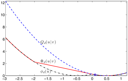
Figure 1: Nonconvex cost function (black, dash point) in (2) against the proposed majorizer (red, solid) in (3) and a vanilla quadratic majorizer (blue, dashed) in (6), for $d=0.5$ and $v=0.1$. The proposed convex majorizer is a much more accurate approximation.

IV-B Majorization function for (1)

Now, for given $x[l]$, consider the function

$$F(x\,|\,x[l])=\sum_{i\sim j}F_{ij}(x_{i},x_{j})+\sum_{i}\sum_{k\in\mathcal{A}_{i}}F_{ik}(x_{i}),$$ (7)

where

$$F_{ij}(x_{i},x_{j}) = \Phi_{d_{ij}}(x_{i}-x_{j}\,|\,x_{i}[l]-x_{j}[l])$$ (8)

and

$$F_{ik}(x_{i}) = \Phi_{r_{ik}}(x_{i}-a_{k}\,|\,x_{i}[l]-a_{k}).$$ (9)

Given Proposition 1, it is clear that it majorizes $f$ and is tight at $x[l]$. Moreover, it is convex as a sum of convex functions.

V Distributed minimization

At the $l$-th iteration of DCOOL-NET, the convex function in (7) must be minimized. We now show how this optimization problem can be solved collaboratively by the network in a distributed, parallel manner.

V-A Problem reformulation

In the distributed algorithm, the working node will operate on local copies of the estimated positions of its neighbors and of itself. So, it is convenient to introduce new variables. Let ${\mathcal{V}}_{i}=\{j\,:\,j\sim i\}$ denote the neighbors of sensor $i$. We also define the closed neighborhood $\overline{\mathcal{V}}_{i}={\mathcal{V}}_{i}\cup\{i\}$. For each $i$, we duplicate $x_{i}$ into new variables $y_{ji}$, $j\in\overline{\mathcal{V}}_{i}$, and $z_{ik}$, $k\in{\mathcal{A}}_{i}$. This choice of notation is not fortuitous: the first subscript reveals which physical node will store the variable, in our proposed implementation; thus, $x_{i}$ and $z_{ik}$ are stored at node $i$, whereas $y_{ji}$ is managed by node $j$. We write the minimization of (7) as the optimization problem

$$\begin{array}[]{ll}\operatornamewithlimits{minimize}&F(y,z)\\ \mbox{subject to }&y_{ji}=x_{i},\qquad j\in\overline{\mathcal{V}}_{i}\\ &z_{ik}=x_{i},\qquad k\in\mathcal{A}_{i},\\ \end{array}$$ (10)

where $y=\{y_{ji}:i\in\mathcal{V},j\in\overline{\mathcal{V}}_{i}\}$, $z=\{z_{ik}:i\in\mathcal{V},k\in\mathcal{A}_{i}\}$, and

$$F(y,z)= \sum_{i\sim j}\left(F_{ij}\left(y_{ii},y_{ij}\right)+F_{ij}\left(y_{ji},y_{jj}\right)\right)+$$ (11)

$$+2\sum_{i}\sum_{k\in\mathcal{A}_{i}}F_{ik}\left(z_{ik}\right).$$

In passing from (7) to (10) we used the identity $F_{ij}(x_{i},x_{j})=\frac{1}{2}F_{ij}\left(y_{ii},y_{ij}\right)+\frac{1}{2}F_{ij}\left(y_{ji},y_{jj}\right)$, due to $y_{ji}=x_{i}$. Also, for convenience, we have rescaled the objective by a factor of two.

V-B Algorithm derivation

Problem (10) is in the form

$$\begin{array}[]{ll}\operatornamewithlimits{minimize}&F(y,z)+G(x)\\ \mbox{subject to }&A(y,z)+Bx=0\end{array}$$ (12)

where $F$ is the convex function in (11), $G$ is the identically zero function, $A$ is the identity operator and $B$ is a matrix whose rows belong to the set $\{-e_{i}^{\top},\>i\in\mathcal{V}\}$, being $e_{i}$ the $i$th column of the identity matrix of size $|\mathcal{V}|$. In the presence of a connected network $B$ is full column rank, so the problem is suited for the Alternating Direction Method of Multipliers (ADMM). See [16] and references therein for more details on this method. See also [17, 18, 19, 20, 21, 22] for applications of ADMM in distributed optimization settings.

Let $\lambda_{ji}$ be the Lagrange multiplier associated with the constraint $y_{ji}=x_{i}$ and $\lambda=\left\{\lambda_{ji}\right\}$ the collection of all such multipliers. Similarly, let $\mu_{ik}$ be the Lagrange multiplier associated with the constraint $z_{ik}=x_{i}$ and $\mu=\{\mu_{ik}\}$. The ADMM framework generates a sequence $\left(y(t),z(t),x(t),\lambda(t),\mu(t)\right)_{t\geq 1}$ such that

$$(y(t+1),z(t+1))=\operatornamewithlimits{argmin}_{y,z}\mathcal{L}_{\rho}\left(y,z,x(t),\lambda(t),\mu(t)\right)$$

(13)

$$x(t+1)=\operatornamewithlimits{argmin}_{x}\mathcal{L}_{\rho}\left(y(t+1),z(t+1),x,\lambda(t),\mu(t)\right)$$

(14)

$$\lambda_{ji}(t+1)=\lambda_{ji}(t)+\rho(y_{ji}(t+1)-x_{i}(t+1))$$ (15)

$$\mu_{ik}(t+1)=\mu_{ik}(t)+\rho(z_{ik}(t+1)-x_{i}(t+1)),$$ (16)

where $\mathcal{L}_{\rho}$ is the augmented Lagrangian defined as

$${\mathcal{L}}_{\rho}(y,z,x,\lambda,\mu)=F(y,z)+\sum_{i}\sum_{j\in\overline{\mathcal{V}}_{i}}\left(\rule{0.0pt}{8.61108pt}\lambda_{ji}^{\top}(y_{ji}-x_{i})+\right.$$

$$\left.\frac{\rho}{2}\left\|y_{ji}-x_{i}\right\|^{2}\rule{0.0pt}{8.61108pt}\right)+\sum_{i}\sum_{k\in{\mathcal{A}}_{i}}\left(\mu_{ik}^{\top}(z_{ik}-x_{i})+\frac{\rho}{2}\left\|z_{ik}-x_{i}\right\|^{2}\right).$$

(17)

Here, $\rho>0$ is a pre-chosen constant.

In our implementation, we let node $i$ store the variables $x_{i}$, $y_{ij}$, $\lambda_{ij}$, $\lambda_{ji}$, for $j\in\overline{\mathcal{V}}_{i}$ and $z_{ik}$, $\mu_{ik}$, for $k\in\mathcal{A}_{i}$. Note that a copy of $\lambda_{ij}$ is maintained at both nodes $i$ and $j$ (this is to avoid extra communication steps). For $t=0$, we can set $\lambda(0)$ and $\mu(0)$ to a pre-chosen constant (e.g., zero) at all nodes. Also, we assume that, at the beginning of the iterations (i.e., for $t=0$) node $i$ knows $x_{j}(0)$ for $j\in{\mathcal{V}}_{i}$ (this can be accomplished, e.g., by having each node $i$ communicating $x_{i}(0)$ to all its neighbors). This property will be preserved for all $t\geq 1$ in our algorithm, via communication steps.

We now show that the minimizations in (13) and (14) can be implemented in a distributed manner and require low computational cost at each node.

VI ADMM: Solving Problem (13)

As shown in Appendix B, the augmented Lagrangian in (17) can be written as

$$\mathcal{L}_{\rho}\left(y,z,x,\lambda,\mu\right) = \sum_{i}\left(\sum_{j\in\overline{\mathcal{V}}_{i}}{\mathcal{L}}_{ij}\left(y_{ii},y_{ij},x_{j},\lambda_{ij}\right)+\right.$$ (18)

$$\left.+\sum_{k\in\mathcal{A}_{i}}{\mathcal{L}}_{ik}\left(z_{ik},x_{i},\mu_{ik}\right)\right)$$

where

$${\mathcal{L}}_{ij}\left(y_{ii},y_{ij},x_{j},\lambda_{ij}\right) = F_{ij}\left(y_{ii},y_{ij}\right)+\lambda_{ij}^{\top}\left(y_{ij}-x_{j}\right)+$$

$$+\frac{\rho}{2}\left\|y_{ij}-x_{j}\right\|^{2}$$

and

$${\mathcal{L}}_{ik}\left(z_{ik},x_{i},\mu_{ik}\right) = 2F_{ik}\left(z_{ik}\right)+\mu_{ik}^{\top}\left(z_{ik}-x_{i}\right)+$$

$$+\frac{\rho}{2}\left\|z_{ik}-x_{i}\right\|^{2}.$$

In (18) we let $F_{ii}\equiv 0$. It is clear from (18) that Problem (13) decouples across sensors $i\in{\mathcal{V}}$, since we are optimizing only over $y$ and $z$. Further, at each sensor $i$, it decouples into two types of subproblems: one involving the variables $y_{ij},j\in\overline{\mathcal{V}}_{i}$, given by

$$\operatornamewithlimits{minimize}_{y_{ij},\>j\in\overline{\mathcal{V}}_{i}} \sum_{j\in\overline{\mathcal{V}}_{i}}{\mathcal{L}}_{ij}\left(y_{ii},y_{ij},x_{j},\lambda_{ij}\right),$$ (19)

and into $|{\mathcal{A}}_{i}|$ subproblems of the form

$$\operatornamewithlimits{minimize}_{z_{ik}} {\mathcal{L}}_{ik}\left(z_{ik},x_{i},\mu_{ik}\right),$$ (20)

involving the variable $z_{ik}$, $k\in\mathcal{A}_{i}$. Note that problems related with anchors are simpler, and, since there are usually few anchors in a network, they do not occur frequently.

VI-A Solving Problem (19)

First, note that node $i$ can indeed address Problem (19) since all the data defining it is available at node $i$: it stores $\lambda_{ji}(t)$, $j\in\overline{\mathcal{V}}_{i}$, and it knows $x_{j}(t)$ for all neighbors $j\in{\mathcal{V}}_{i}$ (this holds trivially for $t=0$ by construction, and it is preserved by our approach, as shown ahead).

To alleviate notation we now suppress the indication of the working node $i$, i.e., variable $y_{ij}$ is simply written as $y_{j}$. Problem (19) can be written as

$$\operatornamewithlimits{minimize}_{y_{j},\>j\in\overline{\mathcal{V}}_{i}} \sum_{j\in\mathcal{V}_{i}}\left(F_{ij}(y_{i},y_{j})+\frac{\rho}{2}\|y_{j}-\gamma_{ij}\|^{2}\right)$$ (21)

$$+\frac{\rho}{2}\|y_{i}-\gamma_{ii}\|^{2},$$

where $\gamma_{ij}=x_{j}-\frac{\lambda_{ij}}{\rho}$.

We make the crucial observation that, for fixed $y_{i}$, the problem is separable in the remaining variables $y_{j}$, $j\in\mathcal{V}_{i}$. This motivates writing (21) as the master problem

$$\operatornamewithlimits{minimize}_{y_{i}}H(y_{i})=\sum_{j\in\mathcal{V}_{i}}H_{ij}(y_{i})+\frac{\rho}{2}\|y_{i}-\gamma_{ii}\|^{2},$$ (22)

where

$$H_{ij}(y_{i})=\min_{y_{j}}F_{ij}(y_{i},y_{j})+\frac{\rho}{2}\|y_{j}-\gamma_{ij}\|^{2}.$$ (23)

We now state important properties of $H_{ij}$.

Proposition 2

Define $H_{ij}$ as in (23). Then:

1. Optimization problem (23) has a unique solution $y_{j}$ for any given $y_{i}$, henceforth denoted $y_{j}^{\star}(y_{i})$;

2. Function $H_{ij}$ is convex and differentiable, with gradient

   $$\nabla H_{ij}(y_{i})=\rho\left(y_{j}^{\star}(y_{i})-\gamma_{ij}\right);$$ (24)

3. The gradient of $H_{ij}$ is Lipschitz continuous with parameter $\rho$, i.e.,

   $$\|\nabla H_{ij}(u)-\nabla H_{ij}(v)\|\leq\rho\|u-v\|$$

   for all $u,v\in{\mathbb{R}}^{p}$.

Proof:

1. Recall from (8) that $F_{ij}(y_{i},y_{j})=\Phi_{d}(y_{i}-y_{j}\,|\,v)$ where $d=d_{ij}$ and $v=x_{i}[l]-x_{j}[l]$. We have $H_{ij}(y_{i})=\Theta(y_{i}-\gamma_{ij})$ where

   $$\Theta(w)=\min_{u}\Phi_{d}(u\,|\,v)+\frac{\rho}{2}\left\|u-w\right\|^{2}.$$ (25)

   Moreover, $u^{\star}$ solves (25) if and only if $y_{j}^{\star}=y_{i}-u^{\star}$ solves (23). Now, the cost function in (25) is clearly continuous, coercive (i.e., it converges to $+\infty$ as $\left\|u\right\|\rightarrow+\infty$) and strictly convex, the two last properties arising from the quadratic term. Thus, it has an unique solution;

2. The function $\Theta$ is the Moreau-Yosida regularization of the convex function $\Phi_{d}(\cdot|v)$ [23, XI.3.4.4]. As $\Theta$ is known to be convex and $H_{ij}$ is the composition of $\Theta$ with an affine map, $H_{ij}$ is convex. It is also known that the gradient of $\Theta$ is

   $$\nabla\Theta(w)=\rho(w-u^{\star}(w))$$

   where $u^{\star}(w)$ is the unique solution of (25) for a given $w$. Thus,

   $$\nabla H_{ij}(y_{i}) = \nabla\Theta(y_{i}-\gamma_{ij})$$

   $$= \rho(y_{i}-\gamma_{ij}-u^{\star}(y_{i}-\gamma_{ij})).$$

   Unwinding the change of variable, i.e., using $y_{j}^{\star}(y_{i})=y_{i}-u^{\star}(y_{i}-\gamma_{ij})$, we obtain (24);

3. Follows from the well known fact that the gradient of $\Theta$ is Lipschitz continuous with parameter $\rho$.

∎

As a consequence, we obtain several nice properties of the function $H$.

Theorem 3

Function $H$ in (22) is strongly convex with parameter $\rho$, i.e., $H-\frac{\rho}{2}\left\|\cdot\right\|^{2}$ is convex. Furthermore, it is differentiable with gradient

$$\nabla H(y_{i})=\rho\sum_{j\in\mathcal{V}_{i}}\left(y_{j}^{\star}(y_{i})-\gamma_{ij}\right)+\rho(y_{i}-\gamma_{ii}).$$ (26)

The gradient of $H$ is Lipschitz continuous with parameter $L_{H}=\rho(|\mathcal{V}_{i}|+1)$.

Proof:

Since $H$ is a sum of convex functions, it is convex. It is strongly convex with parameter $\rho$ due to the presence of the strongly convex term $\frac{\rho}{2}\left\|y_{i}-\gamma_{ii}\right\|^{2}$. As a sum of differentiable functions, it is differentiable and the given formula for the gradient follows from proposition 2. Finally, since $H$ is the sum of $|{\mathcal{V}}_{i}|+1$ functions with Lipschitz continuous gradient with parameter $\rho$ , the claim is proved. ∎

The properties established in Theorem 3 show that the optimization problem (22) is suited for Nesterov’s optimal method for the minimization of strongly convex functions with Lipschitz continuous gradient [24, Theorem 2.2.3]. The resulting algorithm is outlined in Algorithm 2, which is guaranteed to converge to the solution of (22).

Algorithm 2 Nesterov’s optimal method for (22)

1:  $\hat{y}_{i}(0)=y_{i}(0)$

2:  for $s\geq 0$ do

3:     $y_{i}(s+1)=\hat{y}_{i}(s)-\frac{1}{L_{H}}\nabla H(y_{i}(s))$

4:     $\hat{y}_{i}(s+1)=y_{i}(s+1)+\frac{\sqrt{L_{H}}-\sqrt{\rho}}{\sqrt{L_{H}}+\sqrt{\rho}}(y_{i}(s+1)-y_{i}(s))$

5:  end for

VI-B Solving problem (23)

It remains to show how to solve (23) at a given sensor node. Any off-the-shelf convex solver, e.g. based on interior-point methods, could handle it. However, we present a simpler method that avoids expensive matrix operations, typical of interior point methods, by taking advantage of the problem structure at hand. This is important in sensor networks where the sensors have stringent computational resources.

First, as shown in the proof of Proposition 2, it suffices to focus on solving (25) for a given $w$: solving (23) amounts to solving (25) for $w=y_{i}-\gamma_{ij}$ to obtain $u^{\star}=u^{\star}(w)$ and set $y_{j}^{\star}(y_{i})=y_{i}-u^{\star}$.

Note from (3) that $\Phi_{d}(\cdot|v)$ only depends on $v/\left\|v\right\|$, so we can assume, without loss of generality, that $\left\|v\right\|=1$.

From (3), we see that Problem (25) can be rewritten as

$$\begin{array}[]{ll}\operatornamewithlimits{minimize}&r+\frac{\rho}{2}\left\|u-w\right\|^{2}\\ \mbox{subject to }&g_{d}(u)\leq r\\ &h_{d}(v^{\top}u-d)\leq r,\end{array}$$ (27)

with optimization variable $(u,r)$. The Lagrange dual (c.f., for example, [23]) of (27) is given by

$$\begin{array}[]{ll}\operatornamewithlimits{maximize}&\psi(\omega)\\ \mbox{subject to }&0\leq\omega\leq 1,\end{array}$$ (28)

where $\psi(\omega)=\inf\{\Psi(\omega,u)\,:\,u\in{\mathbb{R}}^{n}\}$ and

$$\Psi(\omega,u)=\frac{\rho}{2}\left\|u-w\right\|^{2}+\omega g_{d}(u)+(1-\omega)h_{d}(v^{\top}u-d).$$ (29)

We propose to solve the dual problem (28), which involves the single variable $\omega$, by bisection: we maintain an interval $[a,b]\subset[0,1]$ (initially, they coincide); we evaluate $\dot{\psi}(c)$ at the midpoint $c=(a+b)/2$; if $\dot{\psi}(c)>0$, we set $a=c$, otherwise, $b=c$; the scheme is repeated until the uncertainty interval is sufficiently small.

In order to make this approach work, we must prove first that the dual function $\psi$ is indeed differentiable in the open interval $\Omega=(0,1)$ and find a convenient formula for its derivative. We will need the following useful result from convex analysis.

Lemma 4

Let $X\subset{\mathbb{R}}^{n}$ be an open convex set and $Y\subset{\mathbb{R}}^{p}$ be a compact set. Let $F:X\times Y\rightarrow{\mathbb{R}}$. Assume that $F(x,\cdot)$ is lower semi-continuous for all $x\in X$ and $F(\cdot,y)$ is concave and differentiable for all $y\in Y$. Let $f\,:\,X\rightarrow{\mathbb{R}}$, $f(x)=\inf\{F(x,y)\,:\,y\in Y\}$. Assume that, for any $x\in X$, the infimum is attained at an unique $y^{\star}(x)\in Y$. Then, $f$ is differentiable everywhere and its gradient at $x\in X$ is given by

$$\nabla f(x)=\nabla F(x,y^{\star}(x))$$ (30)

where $\nabla$ refers to differentiation with respect to $x$.

Proof:

This is essentially [23, VI.4.4.5], after one changes concave for convex, lower semi-continuous for upper semi-continuous and $\inf$ for $\sup$. ∎

Now, view $\Psi$ in (29) as defined in $\Omega\times{\mathbb{R}}^{n}$. Is is clear that $\Psi(\omega,\cdot)$ is lower semi-continuous for all $\omega$ (in fact, continuous) and $\Psi(\cdot,u)$ is concave (in fact, affine) and differentiable for all $u$. In fact, some even nicer properties hold.

Lemma 5

Let $\omega\in\Omega$. The function $\Psi_{\omega}=\Psi(\omega,\cdot)$ is strongly convex with parameter $\rho$ and differentiable everywhere with gradient

$$\nabla\Psi_{\omega}(u)=\rho(u-w)+2\omega(u-\pi(u))+(1-\omega)\dot{h}_{d}(v^{\top}u-d)v,$$ (31)

where $\pi(u)$ denotes the projection of $u$ onto the closed ball of radius $d$ centered at the origin. Furthermore, the gradient of $\Psi_{\omega}$ is Lipschitz continuous with parameter $\rho+2$.

Proof:

We start by noting that $g_{d}$ in (4) can be written as $g_{d}(u)=d^{2}_{C}(u)$ where $C$ is the closed ball with radius $d$ centered at the origin, and $d_{C}$ denotes the distance to the closed convex set $C$. It is known that $g_{d}$ is convex, differentiable, the gradient is given by $\nabla g_{d}(u)=2(u-\pi(u))$ and it is Lipschitz continuous with parameter $2$ [23, X.3.2.3]. Also, function $h_{d}$ in (5) is convex and differentiable. Thus, the function $\Psi_{\omega}$ is convex (resp. differentiable) as a sum of three convex (resp. differentiable) functions. It is strongly convex with parameter $\rho$ due to the first term $\frac{\rho}{2}\left\|\cdot-w\right\|^{2}$. The gradient in (31) is clear. Finally, from $|\dot{h}_{d}(r)|-\dot{h}_{d}(s)|\leq 2|r-s|$ for all $r,s$, there holds for any $u_{1},u_{2}$,

$$|\dot{h}_{d}(v^{\top}u_{1}-d)-\dot{h}_{d}(v^{\top}u_{2}-d)|\leq 2|v^{\top}(u_{1}-u_{2})|\leq 2\|u_{1}-u_{2}\|,$$

where $\|v\|=1$ and the Cauchy-Schwarz inequality was used in the last step. We conclude from (31) that, for any $u_{1},u_{2}$,

$$\|\nabla\Psi_{\omega}(u_{1})-\nabla\Psi_{\omega}(u_{2})\|\leq(\rho+2\omega+2(1-\omega))\left\|u_{1}-u_{2}\right\|,$$

i.e., the gradient of $\Psi_{\omega}$ is Lipschtz continuous with parameter $\rho+2$. ∎

Using Lemma 5, we see that the infimum of $\Psi_{\omega}$ is attained at a single $u^{\star}(\omega)$ since it is a continuous, strongly convex function. The derivative of $\psi$ in (28) relies on $u^{\star}(\omega)$, as seen in Lemma 6.

Lemma 6

Function $\psi$ in (28) is differentiable and its derivative is

$$\dot{\psi}(\omega)=g_{d}\left(u^{\star}(\omega)\right)-h_{d}\left(v^{\top}u^{\star}(\omega)-d\right).$$ (32)

Proof:

We begin by bounding the norm of $u^{\star}(\omega)$. From the necessary stationary condition $\nabla\Psi_{\omega}(u^{\star}(\omega))=0$ and (31) we conclude

$$(\rho+2\omega)u^{\star}(\omega)=\rho w+2\omega\pi(u^{\star}(\omega))-(1-\omega)\dot{h}_{d}(v^{\top}u^{\star}(\omega)-d)v.$$ (33)

Since $|\dot{h}_{d}(t)|\leq 2d$ for all $t$ (see (5)), $\left\|\pi(u)\right\|\leq d$ for all $u$, $\left\|v\right\|=1$, and $0\leq\omega\leq 1$, we can bound the norm of the right-hand side of (33) by $\rho\left\|w\right\|+4d$. Thus,

$$\left\|u^{\star}(\omega)\right\| \leq \frac{1}{\rho+2\omega}(\rho\left\|w\right\|+4d)$$

$$\leq \frac{1}{\rho}(\rho\left\|w\right\|+4d)$$

$$= \left\|w\right\|+\frac{4d}{\rho}.$$

Introduce the compact set $U=\{u\in{\mathbb{R}}^{n}\,:\,\left\|u\right\|\leq\|w\|+4d/\rho\}$. The previous analysis has shown that the dual function in (28) can also be represented as $\psi(\omega)=\inf\{\Psi(\omega,u)\,:\,u\in U\}$, i.e., we can restrict the search to $U$ and view $\Psi$ as defined in $\Omega\times U$. We can thus invoke Lemma 4 to conclude that $\psi$ is differentiable and (32) holds. ∎

Finding $u^{\star}(\omega)$

To obtain $u^{\star}(\omega)$ we must minimize $\Psi_{\omega}$. But, given its properties in Lemma 5, the simple optimal Nesterov method, described in Algorithm 2, is also applicable here.

VI-C Solving problem (20)

Note that node $i$ stores $x_{i}(t)$ and $\mu_{ik}(t)$, $k\in{\mathcal{A}}_{i}$. Thus, it can indeed address Problem (20). Problem (20) is similar (in fact, much simpler) than (19), and following the previous steps leads to the same Nesterov’s optimal method. We omit this straightforward derivation.

VII ADMM: Solving Problem (14)

Looking at (17), it is clear that Problem (14) decouples across nodes also. Furthermore, at node $i$ a simple unconstrained quadratic problem with respect to $x_{i}$ must be solved, whose closed-form solution is

$$x_{i}(t+1) = \frac{1}{|\overline{\mathcal{V}}_{i}|+|{\mathcal{A}}_{i}|}\left(\sum_{j\in\overline{\mathcal{V}}_{i}}\left(\frac{1}{\rho}\lambda_{ji}(t)+y_{ji}(t+1)\right)\right.$$ (34)

$$\left.+\sum_{k\in{\mathcal{A}}_{i}}\left(\frac{1}{\rho}\mu_{ik}(t)+z_{ik}(t+1)\right)\right).$$

For node $i$ to carry this update, it needs first to receive $y_{ji}(t+1)$ from its neighbors $j\in{\mathcal{V}}_{i}$. This requires a communication step.

VIII ADMM: Implementing (15) and (16)

Recall that the dual variable $\lambda_{ji}$ is maintained at both nodes $i$ and $j$. Node $i$ can carry the update $\lambda_{ji}(t+1)$ in (15), for all $j\in{\mathcal{V}}_{i}$, since the needed data are available (recall that $y_{ji}(t+1)$ is available from the previous communication step). To update $\lambda_{ij}(t+1)=\lambda_{ij}(t)+\rho(y_{ij}(t+1)-x_{j}(t+1)$, node $i$ needs to receive $x_{j}(t+1)$ from its neighbors $j\in{\mathcal{V}}_{i}$. This requires a communication step.

IX Summary of the distributed algorithm

Our ADMM-based algorithm currently stops after a fixed number of iterations, denoted $T$.

Algorithm 3 Step 2 of DCOOL-NET: position updates

0:  $x[l]$

0:  $x[l+1]$

1:  for $t=0$ to $T-1$ do

2:     for each node $i\in\mathcal{V}$ in parallel do

3:        Solve Problem (19) by minimizing $H$ in (22) with Alg. 2 to obtain $y_{ij}(t+1)$, $j\in\overline{\mathcal{V}}_{i}$

4:        for $k=1$ to $|\mathcal{A}_{i}|$ do

5:           Solve Problem (20) to obtain $z_{ik}(t+1)$

6:        end for

7:        Send $y_{ij}(t+1)$ to neighbor $j\in\mathcal{V}_{i}$

8:        Compute $x_{i}(t+1)$ from (34)

9:        Send $x_{i}(t+1)$ to all $j\in\mathcal{V}_{i}$

10:        Update $\{\lambda_{ji}(t+1),\mu_{ik}(t+1),\>j\in\overline{\mathcal{V}}_{i},k\in{\mathcal{A}}_{i}\}$ as in (15) and (16)

11:     end for

12:  end for

13:  return  $x[l+1]=x(T)$

Algorithm 3 outlines the procedure derived in Secs. V, VI and VII, and corresponds to step 2 of DCOOL-NET (Algorithm 1). Note that, in order to implement step 5 of Algorithm 3, one must adapt Algorithm 2 to the problem at hand.

IX-A Communication load

Algorithm 3 shows two communication steps: step 7 and step 9. At step 7 each node $i$ sends $|\mathcal{V}_{i}|$ vectors in ${\mathbb{R}}^{p}$, each to one neighboring sensor, and at step 9 a vector in ${\mathbb{R}}^{p}$ is broadcast to all nodes in $\mathcal{V}_{i}$. This results in $2TL|\mathcal{V}_{i}|$ communications of ${\mathbb{R}}^{p}$ vectors for node $i$ for the overall algorithm DCOOL-NET. When comparing with SGO in [12], for $T$ iterations, node $i$ sends $T|\mathcal{V}_{i}|$ vectors in ${\mathbb{R}}^{p}$. The increase in communications is the price to pay for the parallel nature of DCOOL-NET.

IX-B Initialization

We note that the tools introduced so far could, in principle, also be used to set up a distributed initialization scheme (i.e., to generate $x[0]$). More precisely, by following the same steps leading to the ADMM formulation, a convex function structured as (7) is amenable to distributed optimization. For example, the ESOCP relaxation, used for initialization in [12] could fall into this template. We leave a more in-depth exploration of this issue to future work.

X Experimental results

X-A General setup

Unless otherwise specified, the generated geometric networks are composed by $4$ anchors and $50$ sensors, with an average node degree, i.e., $\frac{1}{|\mathcal{V}|}\sum_{i\in\mathcal{V}}|\mathcal{V}_{i}|$, of about $6$. In all experiments the sensors are distributed at random and uniformly on a square of $1\times 1$, and anchors are placed, unless otherwise stated, at the four corners of the unit square (to follow [12]), namely, at $(0,0)$,$(0,1)$, $(1,0)$ and $(1,1)$. These properties require a communication range of about $R=0.24$. Since localizability is an issue when assessing the accuracy of sensor network localization algorithms, the used networks are first checked to be generically globally rigid, so that a small disturbance in measurements does not create placement ambiguities. To detect generic global rigidity, we used the methodologies in[14, Sec. 2]. The results for the proposed algorithm DCOOL-NET consider $L=40$ MM iterations, unless otherwise stated.

Measurement noise

Throughout the experiments, the noise model for range distance measurements is

$$d_{ij}=\|x_{i}-x_{j}\|\cdot|n_{ij}|,\quad r_{ik}=\|x_{i}-a_{k}\|\cdot|n_{ik}|,$$ (35)

where $n_{ij},n_{ik}\sim\mathcal{N}(1,\sigma^{2})$ are independent identically distributed Gaussian random variables with mean value $1$ and standard deviation $\sigma$ (specified ahead).

This is the same model used in [12], against which we compare our algorithm. Our choice of benchmark is motivated by simulation results in [12] showing that the method is more accurate than the one proposed in [9]. As discussed in Section II and without loss of generality, we assume $n_{ij}$ affects the edge measurement as a whole, i.e., both $d_{ij}$ and $d_{ji}$ correspond to the same noisy measurement.

Initialization noise

To initialize the algorithms we take the true sensor positions $x^{\star}=\{x_{i}^{\star}\,:\,i\in{\mathcal{V}}\}$ and we perturb them by adding independent zero mean Gaussian noise, according to

$$x_{i}[0]=x_{i}^{\star}+\eta_{i},$$ (36)

where $\eta_{i}\sim\mathcal{N}(0,\sigma_{\mathrm{init}}^{2}I_{p})$ and $I_{p}$ is the identity matrix of size $p\times p$. The parameter $\sigma_{\mathrm{init}}$ is detailed ahead.

Accuracy measure

To quantify the precision of both algorithms we use Root Mean Square Error (RMSE), defined as

$$\mathrm{RMSE}=\sqrt{\frac{1}{|\mathcal{V}|\mathrm{MC}}\sum_{m=1}^{\mathrm{MC}}\mathrm{SE}_{m}},$$ (37)

where

$$\mathrm{SE}_{m}=\|\hat{x}_{m}-x^{\star}\|^{2}$$ (38)

denotes the network-wide squared error obtained at the $m$th Monte Carlo trial, MC is the number of Monte Carlo trials and $\hat{x}_{m}$ is the estimate of the sensors’ positions at the $m$th Monte Carlo trial. We emphasize that Equation (37) gives an accuracy measure per sensor node in the network, and not the overall RMSE. This is useful, not only to compare the performance between networks of different sizes, but also to be able to extract a physical interpretation of the quantity.

X-B Proposed and quadratic majorizers: RMSE vs. initialization noise

We compare the performance of our proposed majorizer in (7) with a standard one built out of quadratic functions, e.g., the one used in [4]. We have submitted a simple source localization problem with one sensor and $4$ anchors to two MM algorithms, each associated with one of the majorization functions. They ran for a fixed number of $30$ iterations. At each Monte Carlo trial, the true sensor positions were corrupted by zero mean Gaussian noise, as in (36), with standard deviation $\sigma_{\mathrm{init}}\in[0.01,1]$. The range measurements are taken to be noiseless, i.e., $\sigma=0$ in (35), in order to create an idealized scenario for direct comparison of the two approaches.

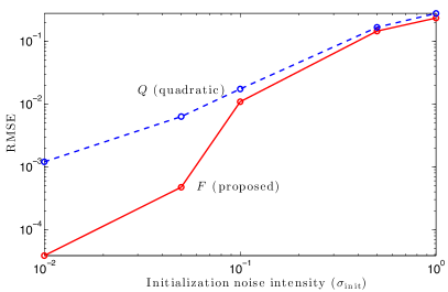
Figure 2: RMSE vs. $\sigma_{\mathrm{init}}$, the intensity of initialization noise in (36). The range measurements are noiseless: $\sigma=0$ in (35). Anchors are at the unit square corners. The proposed majorizer (red, solid) outperforms the quadratic majorizer (blue, dashed) in accuracy.

The evolution of RMSE as a function of initialization noise intensity is illustrated in Fig. 2. There is a clear advantage of using this majorization function when the initialization is within a radius of the true location which is $30\%$ of the square size.

X-C DCOOL-NET and SGO: RMSE vs. initialization noise

Two sets of experiments were made to compare the RMSE performance of SGO in [12] and the proposed DCOOL-NET, as a function of the initialization quality (i.e., $\sigma_{\mathrm{init}}$ in (36)). In the first set, range measurements are noiseless (i.e., $\sigma=0$ in (35)), whereas in the second set we consider noisy range measurements ($\sigma>0$).

X-C1 Noiseless range measurements

In this setup $300$ Monte Carlo trials were run. As the measurements are accurate ($\sigma=0$ in (35)) one would expect not only insignificant values of RMSE, but also a considerable agreement between all the Monte Carlo trials on the solution for sufficiently close initializations.

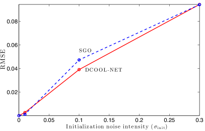
Figure 3: RMSE vs. $\sigma_{\mathrm{init}}$, the intensity of initialization noise in (36). The range measurements are noiseless: $\sigma=0$ in (35). Anchors are at the unit square corners. Proposed DCOOL-NET (red, solid) and SGO (blue, dashed) attain comparable accuracy.

Fig. 3 confirms that both DCOOL-NET and SGO achieve small error positions, and their accuracies are comparable. As stated before, SGO also has a low computational complexity. In fact, lower than DCOOL-NET (although DCOOL-NET is fully parallel across nodes, whereas SGO operates by activating the nodes sequentially, implying some high-level coordination).

TABLE I: Squared error dispersion over Monte Carlo trials for Fig.  3.

$\sigma_{\mathrm{init}}$	DCOOL-NET	SGO
0.01	0.0002	0.0007
0.10	0.0638	0.1290
0.30	0.2380	0.3400

Tab. I shows the squared error dispersion over all Monte Carlo trials, i.e., the standard deviation of the data $\{\mathrm{SE}_{m}\,:\,m=1,\ldots,\mathrm{MC}\}$, recall (38), for both algorithms. We see that DCOOL-NET exhibits a more stable performance, in the sense that it has a lower squared error dispersion.

X-C2 Noisy range measurements

We set $\sigma=0.12$ in the noise model (35).

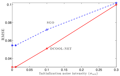
Figure 4: RMSE vs. $\sigma_{\mathrm{init}}$, the intensity of initialization noise in (36). The range measurements are noisy: $\sigma=0.12$ in (35). Anchors are at the unit square corners. Proposed DCOOL-NET (red, solid) outperforms SGO (blue, dashed) in accuracy.

Fig. 4 shows that DCOOL-NET fares better than SGO: the gap between the performances of both algorithms is now quite significant.

TABLE II: Squared error dispersion over Monte Carlo trials for Fig. 4.

$\sigma_{\mathrm{init}}$	DCOOL-NET	SGO
0.00	0.0118	0.0783
0.01	0.0121	0.0775
0.10	0.0727	0.1610
0.30	0.2490	0.3320

The squared error dispersion over all Monte Carlo trials for both algorithms is given in Tab. II. As before, we see that DCOOL-NET is more reliable, in the sense that it exhibits lower variance of estimates across Monte Carlo experiments.

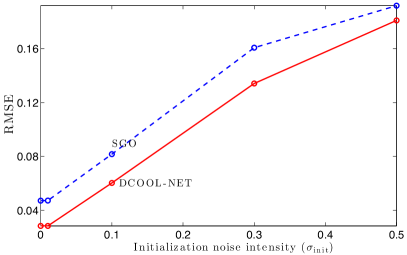
Figure 5: RMSE vs. $\sigma_{\mathrm{init}}$, the intensity of initialization noise in (36). The range measurements are noisy: $\sigma=0.12$ in (35). Anchors were randomly placed in the unit square. Proposed DCOOL-NET (red, solid) outperforms SGO (blue, dashed) in accuracy.

We also considered placing the anchors randomly within the unit square, instead of at the corners. This is a more realistic and challenging setup, where the sensors are no longer necessarily located inside the convex hull of the anchors. The corresponding results are shown in Fig. 5 and Tab. III, for $250$ Monte Carlo trials.

TABLE III: Squared error dispersion over Monte Carlo trials for Fig.  5.

$\sigma_{\mathrm{init}}$	DCOOL-NET	SGO
0.00	0.0097	0.0712
0.01	0.0099	0.0709
0.10	0.1550	0.3160
0.30	0.4350	0.8440
0.50	0.8330	1.3000

Again, DCOOL-NET achieves better accuracy. Comparing the dispersions in Tabs. II and III also reveals that the gap in reliability between SGO and our algorithm is now wider.

X-D DCOOL-NET and SGO: RMSE vs. measurement noise

To evaluate the sensitivity of both algorithms to the intensity of noise present in range measurements (i.e., $\sigma$ in (35)), $300$ Monte Carlo trials were run for $\sigma=0.01,0.1,0.12,0.15,0.17,0.2,0.3$. Both algorithms were initialized at the true sensor positions, i.e., $\sigma_{\mathrm{init}}=0$ in (36), and DCOOL-NET performs $L=100$ iterations.

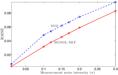
Figure 6: RMSE vs. $\sigma$, the intensity of measurement noise in (35). No initialization noise: $\sigma_{\mathrm{init}}=0$ in (36). Anchors are at the unit square corners. Proposed DCOOL-NET (red, solid) outperforms SGO (blue, dashed) in accuracy.

Fig. 6 and Tab. IV summarize the computer simulations for this setup. As before, DCOOL-NET consistently achieves better accuracy and stability.

TABLE IV: Squared error dispersion over Monte Carlo trials for Fig.  6.

$\sigma$	DCOOL-NET	SGO
0.01	0.0002	0.0016
0.10	0.0177	0.0688
0.12	0.0218	0.0702
0.15	0.0326	0.0921
0.17	0.0394	0.0993
0.20	0.0525	0.1090
0.30	0.1020	0.1630

X-E DCOOL-NET and SGO: RMSE vs. communication cost

We assessed how the RMSE varies with the communication load incurred by both algorithms. We considered the general setup described in Sec. X-A. The results are displayed in Fig. 7. We see an interesting tradeoff: SGO converges much quicker than DCOOL-NET (in terms of communication rounds), and attains a lower RMSE sooner. However, DCOOL-NET can improve its accuracy through more communications, whereas SGO remains trapped in a suboptimal solution.

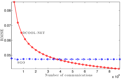
Figure 7: RMSE versus total number of two-dimensional vectors communicated in the network. The range measurements are noiseless: $\sigma=0$ in (35). Initialization is noisy: $\sigma_{\mathrm{init}}=0.1$ in (36). Anchors are at the unit square corners. Proposed DCOOL-NET (red, solid) outperforms SGO (blue, dashed) in accuracy, at the expense of more communications.

X-F DCOOL-NET: RMSE vs. parameter $\rho$

The parameter $\rho$ plays a role in the augmented Lagrangian discussed in Sec. V, and is user-selected. As such, it is important to study the sensitivity of DCOOL-NET to this parameter choice. For this purpose, we have tested several $\rho$ between $1$ and $200$. For each choice, $300$ Monte Carlo trials were performed using noisy measurements and initializations.

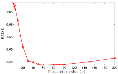
Figure 8: RMSE vs. $\rho$. The range measurements are noisy: $\sigma=0.05$ in (35). Initialization is noisy: $\sigma_{\mathrm{init}}=0.1$ in (36). Anchors are the unit square corners.

Fig. 8 portrays RMSE against $\rho$ for $L=40$ iterations of DCOOL-NET. There is no ample variation, especially for values of $\rho$ over $30$, which offers some confidence in the algorithm resilience to this parameter, a pivotal feature from the practical standpoint. However, an analytical approach for selecting the optimal $\rho$ is beyond the scope of this work, and is postponed for future research. Note that adaptive schemes to adjust $\rho$ do exist for centralized settings, e.g., [16], but seem impractical for distributed setups as they require global computations.

XI Conclusions

Sensor network localization based on noisy range measurement between some pairs of sensors is a current topic of great interest, which maps into a difficult nonconvex optimization problem, once cast in a maximum likelihood (ML) framework. Efficient algorithms guaranteed to find the global minimum are not known even for the centralized setting. In this work, we proposed an algorithm, termed DCOOL-NET, for the more challenging distributed setup in which no central or fusion node is available: instead, neighbor nodes collaboratively exchange messages in order to solve the underlying optimization problem. DCOOL-NET stems from a majorization-minorization (MM) approach and capitalizes on a novel convex majorizer. The proposed majorizer is a main contribution of this work: it is tuned to the nonconvexities of the cost function, which translates into better performance when directly compared with traditional MM quadratic majorizers. More importantly, the new majorizer exhibits several important properties for the problem at hand: it allows for distributed, parallel, optimization via the alternating direction method of multipliers (ADMM) and for low-complexity solvers based on fast-gradient Nesterov methods to tackle the ADMM subproblems at each node. DCOOL-NET decreases the cost function at each iteration, a property inherited from the MM framework, but it is not guaranteed to find the global minimum (a theoretical limitation shared by all existing distributed and non-distributed algorithms). However, computer simulations show that DCOOL-NET achieve better sensor positioning accuracy than a state-of-art method distributed algorithm which, furthermore, is not parallel.

Appendix A Proof of Proposition 1

We write $\Phi_{d}(u)$ instead of $\Phi_{d}(u|v)$ and we let $\langle x,y\rangle=x^{\top}y$.

Convexity

Note that $g_{d}$ is convex as the composition of the convex, non-decreasing function $(\cdot)_{+}^{2}$ with the convex function $\left\|\cdot\right\|-d$. Also, $h_{d}(\langle v/\|v\|,\cdot\rangle-d)$ is convex as the composition of the convex Huber function $h_{d}(\cdot)$ with the affine map $\langle v/\|v\|,\cdot\rangle-d$. Finally, $\Phi_{d}$ is convex as the pointwise maximum of two convex functions.

Tightness

It is straightforward to check that $\phi_{d}(v)=\Phi_{d}(v)$ by examining separately the three cases $\|v\|<d$, $d\leq\|v\|<2d$ and $\|v\|\geq 2d$.

Majorization

We must show that $\Phi_{d}(u)\geq\phi_{d}(u)$ for all $u$. First, consider $\|u\|\geq d$. Then, $g_{d}(u)=\phi_{d}(u)$ and it follows that $\Phi_{d}(v)=\max\{g_{d}(u),h_{d}(\langle v/\|v\|,u\rangle-d)\}\geq\phi_{d}(u)$. Now, consider $\|u\|<d$ and write $u=R\hat{u}$, where $R=\|u\|<d$ and $\|\hat{u}\|=1$. It is straightforward to check that, in terms of $R$ and $\hat{u}$, we have $\phi_{d}(u)=(R-d)^{2}$ and $\Phi_{d}(u)=h_{d}(R\langle\hat{v},\hat{u}\rangle-d)$, where $\hat{v}=v/\|v\|$. Thus, we must show that $h_{d}(R\langle\hat{v},\hat{u}\rangle-d)\geq(R-d)^{2}$. Motivated by the definition of the Huber function $h_{d}$ in two branches, we divide the analysis in two cases.

Case 1: $|R\langle\hat{v},\hat{u}\rangle-d|\leq d$. In this case, $h_{d}(R\langle\hat{v},\hat{u}\rangle-d)=(R\langle\hat{v},\hat{u}\rangle-d)^{2}$. Noting that $|\langle\hat{v},\hat{u}\rangle|\leq 1$, there holds

$$(R\langle\hat{v},\hat{u}\rangle-d)^{2}\geq\inf\{(Rz-d)^{2}\,:\,|z|\leq 1\}=(R-d)^{2},$$

where the fact that $R<d$ was used to compute the infimum over $z$ (attained at $z=1$).

Case 2: $|R\langle\hat{v},\hat{u}\rangle-d|>d$. In this case, $h_{d}(R\langle\hat{v},\hat{u}\rangle-d)=2d|R\langle\hat{v},\hat{u}\rangle-d|-d^{2}$. Thus,

$$h_{d}(R\langle\hat{v},\hat{u}\rangle-d)\geq d^{2}\geq(d-R)^{2},$$

where the last inequality follows from $0\leq R<d$.

Appendix B Proof of (18)

We show how to rewrite (17) as (18). First, note that $F(y,z)$ in (11) can be rewritten as

$$F(y,z)=\sum_{i}\sum_{j\in{\mathcal{V}}_{i}}F_{ij}(y_{ii},y_{ij})+2\sum_{i}\sum_{k\in{\mathcal{A}}_{i}}F_{ik}(z_{ik}).$$ (39)

Here, we used the fact that $F_{ij}(y_{ji},y_{jj})=F_{ji}(y_{jj},y_{ji})$ which follows from $d_{ij}=d_{ji}$ and $\Phi_{d}(u|v)=\Phi_{d}(-u|-v)$, see (3). In addition, there holds

$$\sum_{i}\sum_{j\in\overline{\mathcal{V}}_{i}}\lambda_{ji}^{\top}(y_{ji}-x_{i})+\frac{\rho}{2}\left\|y_{ji}-x_{i}\right\|^{2}$$ (40)

$$= \sum_{j}\sum_{i\in\overline{\mathcal{V}}_{j}}\lambda_{ij}^{\top}(y_{ij}-x_{j})+\frac{\rho}{2}\left\|y_{ij}-x_{j}\right\|^{2}$$

$$= \sum_{i}\sum_{j\in\overline{\mathcal{V}}_{i}}\lambda_{ij}^{\top}(y_{ij}-x_{j})+\frac{\rho}{2}\left\|y_{ij}-x_{j}\right\|^{2}.$$

The first equality follows from interchanging $i$ with $j$. The second equality follows from noting that $i\in\overline{\mathcal{V}}_{j}$ if and only if $j\in\overline{\mathcal{V}}_{i}$. Using (39) and (40) in (17) gives (18).

References

- [1] D. Lai, R. Begg, and M. Palaniswami, Healthcare Sensor Networks: Challenges Toward Practical Implementation. Taylor & Francis, 2011.
- [2] Y. Keller and Y. Gur, “A diffusion approach to network localization,” Signal Processing, IEEE Transactions on, vol. 59, no. 6, pp. 2642 –2654, jun. 2011.
- [3] G. Destino and G. Abreu, “On the maximum likelihood approach for source and network localization,” Signal Processing, IEEE Transactions on, vol. 59, no. 10, pp. 4954 –4970, oct. 2011.
- [4] P. Oguz-Ekim, J. Gomes, J. Xavier, and P. Oliveira, “Robust localization of nodes and time-recursive tracking in sensor networks using noisy range measurements,” Signal Processing, IEEE Transactions on, vol. 59, no. 8, pp. 3930 –3942, aug. 2011.
- [5] P. Biswas, T.-C. Liang, K.-C. Toh, Y. Ye, and T.-C. Wang, “Semidefinite programming approaches for sensor network localization with noisy distance measurements,” Automation Science and Engineering, IEEE Transactions on, vol. 3, no. 4, pp. 360 –371, oct. 2006.
- [6] S. Korkmaz and A.-J. van der Veen, “Robust localization in sensor networks with iterative majorization techniques,” in Acoustics, Speech and Signal Processing, 2009. ICASSP 2009. IEEE International Conference on, apr. 2009, pp. 2049 –2052.
- [7] Y. Shang, W. Rumi, Y. Zhang, and M. Fromherz, “Localization from connectivity in sensor networks,” Parallel and Distributed Systems, IEEE Transactions on, vol. 15, no. 11, pp. 961 – 974, nov. 2004.
- [8] J. Costa, N. Patwari, and A. Hero III, “Distributed weighted-multidimensional scaling for node localization in sensor networks,” ACM Transactions on Sensor Networks (TOSN), vol. 2, no. 1, pp. 39–64, 2006.
- [9] S. Srirangarajan, A. Tewfik, and Z.-Q. Luo, “Distributed sensor network localization using SOCP relaxation,” Wireless Communications, IEEE Transactions on, vol. 7, no. 12, pp. 4886 –4895, dec. 2008.
- [10] F. Chan and H. So, “Accurate distributed range-based positioning algorithm for wireless sensor networks,” Signal Processing, IEEE Transactions on, vol. 57, no. 10, pp. 4100 –4105, oct. 2009.
- [11] U. Khan, S. Kar, and J. Moura, “DILAND: An algorithm for distributed sensor localization with noisy distance measurements,” Signal Processing, IEEE Transactions on, vol. 58, no. 3, pp. 1940 –1947, mar. 2010.
- [12] Q. Shi, C. He, H. Chen, and L. Jiang, “Distributed wireless sensor network localization via sequential greedy optimization algorithm,” Signal Processing, IEEE Transactions on, vol. 58, no. 6, pp. 3328 –3340, jun. 2010.
- [13] D. R. Hunter and K. Lange, “A tutorial on MM algorithms,” The American Statistician, vol. 58, no. 1, pp. 30–37, feb. 2004.
- [14] B. D. O. Anderson, I. Shames, G. Mao, and B. Fidan, “Formal theory of noisy sensor network localization,” SIAM Journal on Discrete Mathematics, vol. 24, no. 2, pp. 684–698, 2010.
- [15] P. Forero and G. Giannakis, “Sparsity-exploiting robust multidimensional scaling,” Signal Processing, IEEE Transactions on, vol. 60, no. 8, pp. 4118 –4134, aug. 2012.
- [16] S. Boyd, N. Parikh, E. Chu, B. Peleato, and J. Eckstein, “Distributed optimization and statistical learning via the alternating direction method of multipliers,” Foundations and Trends® in Machine Learning, vol. 3, no. 1, pp. 1–122, 2011.
- [17] I. Schizas, A. Ribeiro, and G. Giannakis, “Consensus in ad hoc WSNs with noisy links — part i: Distributed estimation of deterministic signals,” Signal Processing, IEEE Transactions on, vol. 56, no. 1, pp. 350 –364, jan. 2008.
- [18] H. Zhu, G. Giannakis, and A. Cano, “Distributed in-network channel decoding,” Signal Processing, IEEE Transactions on, vol. 57, no. 10, pp. 3970 –3983, oct. 2009.
- [19] P. Forero, A. Cano, and G. Giannakis, “Consensus-based distributed support vector machines,” The Journal of Machine Learning Research, vol. 11, pp. 1663–1707, 2010.
- [20] J. Bazerque and G. Giannakis, “Distributed spectrum sensing for cognitive radio networks by exploiting sparsity,” Signal Processing, IEEE Transactions on, vol. 58, no. 3, pp. 1847 –1862, mar. 2010.
- [21] T. Erseghe, D. Zennaro, E. Dall’Anese, and L. Vangelista, “Fast consensus by the alternating direction multipliers method,” Signal Processing, IEEE Transactions on, vol. 59, no. 11, pp. 5523 –5537, nov. 2011.
- [22] J. Mota, J. Xavier, P. Aguiar, and M. Puschel, “Distributed basis pursuit,” Signal Processing, IEEE Transactions on, vol. 60, no. 4, pp. 1942 –1956, apr. 2012.
- [23] J.-B. Hiriart-Urruty and C. Lemaréchal, Convex analysis and minimization algorithms. Springer-Verlag Limited, 1993.
- [24] Y. Nesterov, Introductory Lectures on Convex Optimization: A Basic Course. Kluwer Academic Publishers, 2004.