Non-steady relaxation and critical exponents at the depinning transition

Abstract

We study the non-steady relaxation of a driven one-dimensional elastic interface at the depinning transition by extensive numerical simulations concurrently implemented on graphics processing units. We compute the time-dependent velocity and roughness as the interface relaxes from a flat initial configuration at the thermodynamic random-manifold critical force. Above a first, non-universal microscopic time regime, we find a non-trivial long crossover towards the non-steady macroscopic critical regime. This “mesoscopic” time regime is robust under changes of the microscopic disorder, including its random-bond or random-field character, and can be fairly described as power-law corrections to the asymptotic scaling forms yielding the true critical exponents. In order to avoid fitting effective exponents with a systematic bias we implement a practical criterion of consistency and perform large-scale ($L\simeq 2^{25}$) simulations for the non-steady dynamics of the continuum displacement quenched Edwards-Wilkinson equation, getting accurate and consistent depinning exponents for this class: $\beta=0.245\pm 0.006$, $z=1.433\pm 0.007$, $\zeta=1.250\pm 0.005$, and $\nu=1.333\pm 0.007$. Our study may explain numerical discrepancies (as large as $30\%$ for the velocity exponent $\beta$) found in the literature. It might also be relevant for the analysis of experimental protocols with driven interfaces keeping a long-term memory of the initial condition.

I Introduction

The depinning transition of an elastic interface driven in a random medium is a paradigmatic example of universal out-of-equilibrium dynamical behavior in disordered systems kardar_review_lines ; Fisher_review_collective_transport . From a purely theoretically point of view, considerable progress has been made in the last years thanks to a fruitful interplay between the very powerful analytical fisher_functional_rg ; chauve_creep_long ; ledoussal_frg_twoloops and numerical techniques specially developed for studying equilibrium huse_henley_polymer_equilibrium ; kardar_polymer_equilirium , depinning leschhorn_automaton ; rosso_roughness_MC ; rosso_dep_exponent ; rosso_depinning_longrange_elasticity ; olaf_std_longrangedepinning , and creep kolton_depinning_zerot2 ; kolton_dep_zeroT_long of strictly elastic manifolds. From the experimental viewpoint, on the other hand, the understanding of this particular problem is directly relevant for various experimental situations where the elastic approximation is well met, such as magnetic  lemerle_domainwall_creep ; bauer_deroughening_magnetic2 ; yamanouchi_creep_ferromagnetic_semiconductor2 ; metaxas_depinning_thermal_rounding or ferroelectric domain walls paruch_ferro_roughness_dipolar ; paruch_ferro_quench ; ferroelectric_zombie_paper ; paruchbusting , contact lines in wetting moulinet_distribution_width_contact_line2 ; frg_exp_contactline , and fractures bouchaud_crack_propagation2 ; alava_review_cracks . It has also been useful for making a connection between laboratory friction experiments and the observed spatial and temporal earthquake clustering jagla_kolton_earthquakes . In spite of this progress, classifying the above systems in depinning universality classes remains, in most cases, a challenge. In this respect, we show in this paper that a detailed understanding of the experimentally relevant non-stationary dynamics at the depinning transition can be useful.

The physics of an elastic interface in a random medium is controlled by the competition between quenched disorder (induced by the presence of impurities in the host material), which promotes the wandering of the elastic object, and the elastic forces, which tend to make the object flat. One of the most dramatic manifestations of this competition is the response of these systems to an external drive, particularly the depinning transition phenomenon. In the absence of an external drive, the ground state of the system is disordered but well characterized by a self-affine rough geometry with a diverging typical width $w\sim L^{\zeta_{\mathrm{eq}}}$, where $L$ is the linear size of the elastic object and $\zeta_{\mathrm{eq}}$ is the equilibrium roughness exponent. When the external force is increased from zero, the ground state becomes unstable and the interface is locked in metastable states. To overcome the barriers separating them and reach a finite steady-state velocity $v$ it is necessary to exceed a finite critical force, above which barriers disappear and no metastable states exist. For directed $d$-dimensional elastic interfaces with convex elastic energies in a ($D=d+1$)-dimensional finite space with disorder, the critical point is unique, characterized by the critical force $f=f_{c}$ and its associated critical configuration middleton_theorem ; rosso_roughness_at_depinning . This critical configuration is also rough and self-affine such that $w\sim~{}L^{\zeta}$ with $\zeta$ the depinning roughness exponent. When approaching the threshold from above, the steady-state average velocity vanishes as $v\sim(f-f_{c})^{\beta}$ and the correlation length characterizing the cooperative avalanche-like motion diverges as $\xi\sim(f-f_{c})^{-\nu}$ for $f>f_{c}$ with a typical diverging inter-event time $\xi^{z}$, where $\beta$ is the velocity exponent, $\nu$ is the depinning correlation length exponent, and $z$ is the dynamical exponent fisher_depinning_meanfield ; narayan_fisher_cdw ; nattermann_stepanow_depinning ; ledoussal_frg_twoloops . At finite temperature and for $f\ll~{}f_{c}$, the system presents an ultra-slow steady-state creep motion with universal features ioffe_creep ; vinokur_creep_argument ; chauve_creep_long directly correlated with geometrical crossovers kolton_creep2 ; kolton_depinning_zerot2 . At very small temperatures the monotonic increase of the correlation length with decreasing $f$ below $f_{c}$ shows that the naive analogy breaks, and that depinning must be regarded as a non-standard phase transition kolton_depinning_zerot2 ; kolton_dep_zeroT_long . The transition is then smeared-out, with the velocity vanishing as $v\sim T^{\psi}$ exactly at $f=f_{c}$, with $\psi$, the so-called thermal rounding exponent chen_marchetti ; nowak_thermal_rounding ; bustingorry_thermal_rounding_epl ; bustingorry_thermal_depinning_exponent ; bustingorry_thermal_rounding_fitexp .

The non-stationary dynamics at depinning is a different and interesting manifestation of the competition between elasticity and disorder, but it has received considerably less attention than the steady-state dynamics. Near the threshold the time needed to reach the driven non-equilibrium steady state can be very long, since the memory of the initial condition persists for length scales larger than a growing correlation length $\ell(t)\sim t^{1/z}$. Being limited only by the divergent steady-state correlation length $\xi$ and the system size $L$, the resulting non-steady critical regime is macroscopically large, $t\lesssim\xi^{z},L^{z}$ . It is hence relevant for experimental protocols, where it is in general difficult to assure history independence, as the memory of the initial condition is erased only by this slow transient process. Analogously to non-driven systems relaxing to their critical equilibrium states cugliandolo_glassy_review , the transient dynamics of a driven disordered system displays interesting, though different, universal features kolton_universal_aging_at_depinning .

In this paper we study the non-steady relaxation of an elastic string in a random medium by extensive numerical simulations, extending the study of Ref. kolton_short_time_exponents in several ways. We first show that the thermodynamic critical force, although strictly non-universal, can be defined unambiguously and has a unique value; this is the force that drives the system into the so-called short-time-dynamics (STD) scaling form yielding the steady-state critical exponents. Second, we study corrections to the dynamical scaling form which appear at intermediate (“mesoscopic”) times, but well above the expected non-universal microscopic time regime set by the microscopic disorder correlation range. We show that these corrections are rather robust under changes of the microscopic disorder, including its random-bond or random-field character. Having done this, we implement a practical criterion for separating these corrections and exploit the parallelism of graphics processing unit (GPU) computing to perform, to the best of our knowledge, the largest-to-date molecular dynamics simulations of an elastic line in a random-medium described by a continuous quenched Edwards-Wilkinson (QEW) equation. This allows us to achieve long times in the non-steady critical regime and get, with the STD method, un-biased and precise estimates for the critical exponents for this depinning universality class: $\beta=0.245\pm 0.006$, $z=1.433\pm 0.007$, $\zeta=1.250\pm 0.005$, and $\nu=1.333\pm 0.007$.

Organization of the paper

In Sec. II we define the model and quantities of interest. In Sec. III.1 we describe the general scaling forms for the non-steady critical relaxation that are used for the analysis. In Sec. III.2 we briefly discuss the numerical methods, leaving all computational details for the Supplemental Material supplementalmaterial . In Sec. IV we show all the results. We first analyze the geometry of the critical configuration and the thermodynamic limit of the critical force in Sec. IV.1. Then we study the non-steady relaxation of different observables in Sec. IV.2. We characterize in Sec. IV.3 the deviations from the expected scaling forms of Sec. III.1, and in Sec. IV.4 we analyze in detail these corrections to scaling, which explain the existence of biased effective exponents in the problem. In Sec. V we summarize and discuss all the results and in Sec. VI we conclude and give perspectives.

II Models, Protocols, and Observables

We study a one-dimensional elastic line described by a single-valued function $u(x,t)$. Here, $u(x,t)$ measures the line’s instantaneous transverse displacement from the $x$ axis at time $t$. In the continuum, the overdamped interface dynamics is described by the QEW equation of motion,

$$\eta\partial_{t}u(x,t)=c\partial_{x}^{2}u(x,t)+F_{p}(u,x)+f,$$ (1)

where $f$ is a uniformly applied external force and $F_{p}(u,x)$ is the random pinning force. Without lack of generality we can set the friction coefficient $\eta=1$ and the elastic constant $c=1$. The pinning force has zero average and correlator

$$\overline{F_{p}(u,x)F_{p}(u^{\prime},x^{\prime})}=\Delta(u-u^{\prime})\delta(x-x^{\prime}).$$ (2)

The overbar represents the average over the disorder realizations and $\Delta(u)$ is a short-ranged function, of range $r_{f}=1$. We consider two cases for $\Delta(x)$. In the so-called random bond (RB) case the elastic line moves in a random potential such that $F_{p}(u,x)=-\partial_{u}U(u,x)$ with $U(u,x)$ bounded, and thus $\int_{u}\Delta(u)=0$. In the random field (RF) case, the random potential $U(u,x)$ is unbounded and diffuses as a function of $u$, with diffusion constant $\int_{u}\Delta(u)>0$ chauve_creep_long . In turn, the pinning potential or forces can be sampled from different distributions. Here we consider Gaussian and uniform (constant) distributions. Analyzing all the above cases separately will allow us to detect possible departures from the expected universal behavior and corrections to scaling at relatively short time and length scales.

It is a convenient and safe procedure to discretize the interface displacement in the $x$-direction, keeping $u(x,t)$ as a continuum variable. Doing so, we define the center of mass velocity for an interface of size $L$ as,

$$v(t)=\overline{\frac{1}{L}\sum_{x=0}^{L-1}\partial_{t}u(x,t)},$$ (3)

which, given Eq. (1) and $\eta=c=1$, is nothing else but the spatial average of the instantaneous total forces acting on the line. From the instantaneous center of mass displacement,

$$u(t)=\overline{\frac{1}{L}\sum_{x=0}^{L-1}u(x,t)},$$ (4)

we can define the instantaneous quadratic width of the interface as,

$$w^{2}(t)=\overline{\frac{1}{L}\sum_{x=0}^{L-1}[u(x,t)-u(t)]^{2}}.$$ (5)

The geometrical properties of the line as a function of length-scale can be conveniently described using the averaged structure factor

$$S_{q}(t)=\overline{\biggl{|}\frac{1}{L}\sum_{x=0}^{L-1}u(x,t)e^{-iqx}\biggr{|}^{2}},$$ (6)

where $q=2\pi n/L$, with $n=1,\ldots,L-1$.

We are interested in the time dependence of the above disorder-averaged observables with the elastic line initially flat, i.e., $u(x,t=0)=0$. Other, more complex, initial conditions may also be considered, but they do not provide more information on the dynamics of relaxation as long as they are not correlated with the random potential. Choosing an initially flat line allows us to easily detect the existence of memory depending on the length-scale, since correlations in this system always develop a roughness with self-affine length regimes described by positive exponents. For a globally self affine line we have $S(q)\sim q^{-(1+2\zeta)}$, thus yielding the roughness exponent $\zeta$. Such behavior is expected to hold in the so-called random-manifold regime; a regime where $q$ is small compared to both the Larkin wavevector $q_{c}\sim\ell_{c}^{-1}$, [with $w(\ell_{c})\sim r_{f}$] and the discretization wave vector $q_{d}\sim 1$. For our parameters, we have $q_{c}\sim q_{d}$ of order $O(1)$.

III Methods

We describe here the scaling forms expected for the non-stationary relaxation of an elastic line in a random medium at large times, and introduce the numerical methods used to simulate the dynamics.

III.1 Universal non-steady relaxation

It was originally shown JaScSc1989 using renormalization group techniques for a type A model, and then widely extended empirically to other models, that the short-time behavior of the order parameter’s $n$-th moment close to a critical point follows the universal scaling relation

$$m^{(n)}(t,h,L,m_{0})=b^{-n\beta/\nu}m^{(n)}(b^{-z}t,b^{1/\nu}h,b^{-1}L,b^{\mu}m_{0}).$$ (7)

Here $t$ is the time, $h=(H-H_{c})/H_{c}$ is the reduced driving field of the transition associated with the order parameter (such as magnetic field, temperature, etc.), $L$ is the system size, $b$ is a scaling factor, $m_{0}$ is the order parameter’s initial value, $\mu$ is a universal exponent associated with the short-time behavior, while $\beta$, $\nu$, and $z$ are the usual critical and dynamical exponents. This relation was analytically shown to be valid in the limit of small initial order parameter $m_{0}\ll 1$, with $t$ larger that some non-universal microscopic time and smaller than the equilibration time $\tau_{\tt eq}\sim L^{z}$. Nevertheless, in agreement with numerical simulations Zh1998 ; Zh2006 ; review_albano and analytical approximations in mean-field models AnFeCa2010 , it was shown that the following homogeneity relation is valid in the short (but macroscopic) time regime when starting from an ordered condition (commonly $m_{0}=1$).

$$m^{(n)}(t,h,L)=b^{-n\beta/\nu}m^{(n)}(b^{-z}t,b^{1/\nu}h,b^{-1}L).$$ (8)

In our system, and making the usual analogy with standard phase transitions, we consider the velocity $v$ as an order parameter and the adimensionalized force $(f-f_{c})/f_{c}$ as the reduced driving field. While it is not clear yet how to implement a protocol yielding an initial condition equivalent to $m_{0}\ll 1$ and testing the complete relation Eq. (7), the implementation of an ordered equivalent initial condition is very simple, and a relation like Eq. (8) has been numerically checked in this model kolton_short_time_exponents ; kolton_universal_aging_at_depinning . In fact, the completely ordered initial condition should correspond to the infinite-velocity configuration. Since at large velocities the effect of the quenched disorder mimics a small thermal noise which vanishes with increasing $v$, this initial condition should correspond to the completely flat condition (i.e., we make a “quench” from an infinite to a finite force). By analogy, we therefore expect the velocity short-time behavior

$$v(t,h,L)=b^{-\beta/\nu}\tilde{\tilde{v}}_{\pm}(b^{-z}t,b^{1/\nu}h,b^{-1}L),$$ (9)

where $h=|f-f_{c}|/f_{c}$ and the function $\tilde{\tilde{v}}_{\pm}$ has two branches depending on the sign of $f-f_{c}$. By choosing $b=t^{1/z}$ in (9),

$$v(h,L,t)=t^{-\beta/\nu z}\tilde{v}_{\pm}(t^{1/z\nu}h,t^{-1/z}L),$$ (10)

Here, the functions $\tilde{v}_{+}$ and $\tilde{v}_{-}$ are such that for $h>0$ and $L\gg h^{-\nu}$, $v_{+}\to\tt{const}$ and $v_{-}\to 0$ in the large $t$ limit. It is worth noting here that while $h^{-\nu}$ can be associated with the geometrical correlation length $\xi$ diverging in $\lim f\to f_{c}^{+}$ in the steady state, this is not true in $\lim f\to f_{c}^{-}$. We can, however, find a divergent correlation length $\ell_{\tt relax}\sim(f_{c}-f)^{-\nu}$, not observed in the steady-state geometry, but associated with the deterministic part of the avalanches that are produced in the steady-state dynamics of the $f<f_{c}$ low-temperature creep regime kolton_depinning_zerot2 ; kolton_dep_zeroT_long . Hence, the interpretation of Eq. (10) is slightly different from the one derived from Eq. (8) for the Ising model (and other similar standard phase transitions), where divergent equilibrium correlation lengths do exist on approaching the critical point from both sides. At depinning, the relaxational dynamics described by Eq. (10) is valid in the short-time regime, after which the velocity reaches a steady-state value if $f>f_{c}$, while for $f<f_{c}$ the velocity is blocked in a metastable state with memory of the initial condition and $v\to 0$ kolton_short_time_exponents . When $T>0$, and for $f<f_{c}$, activated processes permit the system to continue relaxing towards a steady-state with finite velocity bustingorry_thermal_depinning_exponent .

Exactly at the critical point ($h=0$) and in the limit $L\to\infty$ we expect a power-law behavior for the velocity,

$$v\sim t^{-\beta/\nu z}.$$ (11)

Equation (11) can also be heuristically derived from a very simple physical picture, by assuming that the non-steady relaxation at the critical point is controlled by a single growing correlation length $\ell(t)\sim t^{1/z}$, and that in the macroscopic time limit, some critical steady-state relations are “instantaneously” obeyed, with $\ell(t)$ playing the role of $\xi$, when $\xi\ll L$. Hence, the steady-state relation $v\sim\xi^{-\beta/\nu}$ translates into $v\sim\ell(t)^{-\beta/\nu}\sim t^{-\beta/\nu z}$, leading to Eq. (11). The physical picture behind this “mapping” is that length scales below $\ell(t)$ are expected to be steady-state quasi-equilibrated, while above it the memory of the initical condition is still kept. This suggests that the structure factor should be described, above some microscopic scale and for $\ell(t)\ll L$, by

$$S_{q}(t)\sim q^{-(1+2\zeta)}\tilde{\tilde{S}}(q\ell(t))\sim q^{-(1+2\zeta)}\tilde{S}(qt^{1/z}),$$ (12)

with $\tilde{S}(y)\sim{\tt const}$ for $y\gg 1$, and $\tilde{S}(y)\sim y^{1+2\zeta}$ for $y\ll 1$. This is confirmed by numerical simulations kolton_short_time_exponents ; kolton_universal_aging_at_depinning . Note that this simple scaling is also obeyed in the absence of disorder but in the presence of thermal noise. For the depinning transition $\tilde{S}(y)$ is expected to be a much more complicated function however, as the disorder in principle couples all Fourier modes. The above scaling relation also implies

$$w(t)\sim\ell(t)^{\zeta}\sim t^{\zeta/z}$$ (13)

for the global width, or roughness. Note that this simple result depends on the choice of a flat initial condition. Otherwise we would have a memory contribution, which can be included as $w(t)\sim t^{\zeta/z}\tilde{w}(t^{1/z}L^{-1})$, with $\tilde{w}(y)\sim{\tt const}$ for $y\leq 1$, and a function depending on the initial condition for $y\ll 1$. The flat initial condition is thus convenient since $\tilde{w}(y)={\tt const}$ for all $y$.

Since Eq. (11) is valid exactly at $h=0$, by evolving the system at different driving forces from a flat initial condition it is then possible to determine the critical force and extract the steady-state critical exponents. For the correct application of this STD method, we need, however, a good criterion to decide the time range in which to fit the exponents accurately. This is particularly tricky if scaling corrections are important and also described by power laws, since they can lead to effective power-law decays, yielding biased incorrect exponents. As we show later on, for our case, we can exploit known depinning scaling relations and combinations of observables to find a good criterion.

III.2 Numerical simulation

The numerical simulation protocol is roughly the same as the one used in Ref. kolton_short_time_exponents , but here, in addition, we simulate different kinds of disorder, and implement massively parallel algorithms. Below we briefly summarize the method. We refer the reader to the Supplemental Material supplementalmaterial for further details; in particular, for the description of our GPU-based parallel implementations of the algorithm which allow us to computationally reach very large system sizes, running simulations with speedups above 300x.

In order to numerically solve Eq. (1) the system is discretized in the $x$ direction into $L$ segments of size $\delta x=1$, i.e., $x=0,\ldots,L-1$, while keeping $u(x,t)$ as a continuous variable. Computing the forces at each time-step, the integration of Eq. (1) is done using the Euler method.

To model the continuous quenched random potential we can either read from a precomputed array, or generate dynamically, uncorrelated random numbers with a finite variance at the integer values of $u$ and $x$ and use interpolation to get $F_{p}(u,x)$. In this work we consider both cubic-spline and linear interpolation between the random potential values sampled at the integers. This changes only the shape of the microscopic force correlator, but not the universality class. By generating directly the force field at integer positions from zero-mean uncorrelated random numbers in both directions we can get a RF disorder, while by doing the same for the potential field and deriving the force we can get a RB disorder. In both cases Eq. (2), with a short-range force correlator, is automatically satisfied.

For our numerical simulations we have used periodic boundary conditions in the longitudinal direction, so that $u(0,t)$ is elastically coupled with $u(L-1,t)$. In the case where we construct continuous splines for the disorder potential or we limit ourselves to read a precomputed force field, we enforce periodic boundary conditions also in the transverse direction, thus defining an $L\times M$ system. On the other hand, when a dynamically generated disorder is used, the system size in the $u$ direction is virtually infinite, although in our implementation it can be forced to be periodic as well supplementalmaterial .

A critical configuration $u^{s}_{c}(x)$ and a critical force $f^{s}_{c}$ can be unambiguously defined for a periodic sample of size $L\times M$ and with a given disorder realization. They are defined from the pinned (zero-velocity) configuration with the largest driving force $f$ in the long time limit dynamics. They are the real solutions of

$$c\,\partial^{2}_{z}u(x)+F_{p}(u,x)+f=0,$$ (14)

such that for $f>f^{s}_{c}$ there are no further real solutions (pinned configurations). Middleton theorems middleton_theorem can be used to devise an efficient algorithm which allows the critical force $f^{s}_{c}$ and the critical configuration $u^{s}_{c}(x)$ to be obtained for each independent disorder realization iteratively, without having to solve the actual dynamics Eq. (1) nor directly invert the non-linear system of Eq. (14). In the following section we use such an algorithm rosso_dep_exponent ; rosso_depinning_longrange_elasticity to study the finite-size effects on $f^{s}_{c}$ and in particular to obtain the appropriate thermodynamic limit $f_{c}=\lim_{(L,M)\to\infty}\overline{f^{s}_{c}}$ controlling the universal non-steady relaxation.

IV Results

IV.1 The critical configuration and the thermodynamic critical force

We start by analyzing the geometry of the critical configuration and the critical force in periodic samples of size $L\times M$, using the exact algorithm of Refs. rosso_dep_exponent ; rosso_depinning_longrange_elasticity , for a cubic-spline RB potential. This allows us, on one hand, to get a very precise estimate for the exponent $\zeta$ directly from steady-state solutions for individual samples $u^{s}_{c}(x)$ and use it to disentangle the combinations of exponents appearing in the non-steady universal part of the relaxation. On the other hand, it allows us to get the value $f_{c}$ for the thermodynamic critical force, and show, from an anisotropic finite-size analysis, that it is unambiguously defined. In the next section we show that the results obtained in this section are fully consistent with the non-steady dynamics: The long-time geometry tends to the self-affine one of the critical configuration and, in particular, $f_{c}$ is exactly the force for which the velocity relaxation asymptotically displays a power-law decay in time, as long as the growing correlation length remains smaller than the system size $L$

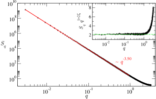
Figure 1: (Color online) Structure factor of the critical configuration averaged over $N=1000$ samples of size $L=2048$ and $M=13777$. Using the self-affinity developed at long wavelengths, $S(q)\sim q^{-(1+2\zeta)}$, we fit the roughness exponent $\zeta=1.250\pm 0.005$. Inset: Rescaled structure factor qualitatively displaying the accuracy of the fit, and the discretization effects at large $q$.

We determine the critical configurations $u^{s}_{c}(x)$ and the associate critical force $f^{s}_{c}(L,M)$, for several samples of size $L\times M$. To determine $\zeta$ we calculate the time-independent averaged structure factor $S_{q}$ of the critical configurations and fit the expected $S_{q}\sim q^{-(1+2\zeta)}$ behavior. The advantage of using $S_{q}$ over the global width $w(L)\sim L^{\zeta}$ is that it allows us to better detect the possible presence of undesirable crossover effects, and the characteristic associated length-scale. In particular, when determining $\zeta$, one should be cautious about the crossover to the random-periodic regime, with exponent $\zeta_{\tt RP}=1.5$ occurring at the length-scale $L_{M}\sim M^{1/\zeta}$ bustingorry_periodic . In our case we have thus chosen $M\gtrsim L^{\zeta}$ for extracting $\zeta$. In Fig. 1 we observe that $S_{q}\sim q^{-(1+2\zeta)}$ holds to high accuracy in the long wavelength limit (discretization effects appear at very short wavelengths) for a system of size $L=2048$ and $M=13777$. From a power-law fitting giving $1+2\zeta=3.50\pm 0.01$ we deduce $\zeta=1.250\pm 0.005$, with better precision but still in very good agreement with previous estimates obtained with the structure factor at finite velocities in the steady-state duemmer2 and with the scaling of the global width $w(L)\sim L^{\zeta}$ leschhorn_automaton ; rosso_roughness_at_depinning .

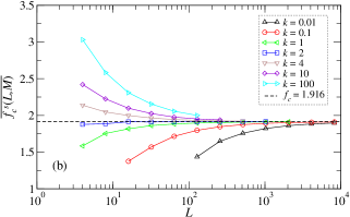
Figure 2: (Color online) Dependence of the finite-size critical force $\overline{f^{s}_{c}}$ on the longitudinal size $L$ for periodic samples of size $L\times M$ with $M=kL^{\zeta}$. The dashed line corresponds to the thermodynamic limit $f_{c}=1.916\pm 0.001$.

In order to study the thermodynamic limit of the disorder averaged critical force, $\overline{f^{s}_{c}(L,M)}$, we use $M=kL^{\zeta}$, with $k$ a finite control parameter. Any finite value of $k$ leads to a parametrized family of universal critical force distributions, ranging from the Gaussian to the Gumbel distribution bolech_critical_force_distribution . For our present purposes, it is important to know how the thermodynamic limit $L\to\infty$ depends on the aspect-ratio parameter $k$. In Fig. 2 we show $\overline{f^{s}_{c}}$ against $L$, for different values of $k$. As we can see, the size-dependent average critical force $\overline{f^{s}_{c}}$ tends to a unique value in the limit $L\to\infty$ when keeping $k$ fixed. Furthermore, at finite $L$, $\overline{f^{s}_{c}}$ is smaller than $f_{c}$ for $k\lesssim 2$, and larger than $f_{c}$ for $k\gtrsim 2$, where $f_{c}$ therefore represents the thermodynamic critical force. This behavior is consistent with the crossover from a random-periodic depinning ($k\to 0$), with a thermodynamic critical force smaller than the random-manifold one, towards the extreme-statistics random-manifold depinning with an infinite thermodynamical critical force ($k\to\infty$), with fluctuations described by the Gumbel distribution bolech_critical_force_distribution ; fedorenko_frg_fc_fluctuations . What is important to remark here nextpaper is that for the whole range of finite values of $k$ that we have analyzed, the curves slowly converge to the same thermodynamic limit $f_{c}=\lim_{(L,M)\to\infty}\overline{f^{s}_{c}}|_{M=kL^{\zeta}}=1.916\pm 0.001$. This value is in very good agreement with the value obtained for the same microscopic model with other methods, such as quasi-statically pulling the string with a soft spring rosso_correlator_RB_RF_depinning .

Therefore, we see that although $f_{c}$ is not universal, for fixed microscopic disorder correlations it attracts the infinite family of sample geometries that is compatible with the random-manifold setting $M=kL^{\zeta}$. Therefore, this setting alone removes the ambiguity of defining the critical force of a periodic sample in the thermodynamic limit. Since the short-time relaxation of the string is controlled by a single growing correlation length $\ell(t)\sim t^{1/z}$ describing the slow development of correlations from microscopic scales, it can not be sensitive to the dimensions or aspect ratio of the computational box, provided that $\ell(t)\ll L$ and $\ell(t)^{\zeta}\ll M$. It is then natural to expect that $f_{c}$, which is sensitive only to the microscopic pinning correlator for the random-bond family $M=kL^{\zeta}$, is the force that must be tuned to target the universal non-steady relaxation regime.

IV.2 Short-time-dynamics scaling

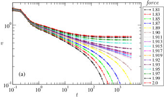
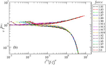
Figure 3: (Color online) Non-stationary averaged string velocity as a function of time for different driving forces. (a) Raw data. The best power-law curve corresponds to $f=f_{c}^{\tt STD}=1.915$. (b) Rescaled data. The parameters $f_{c}^{\tt STD}=1.915$, $\beta=0.33$, $z=1.5$, and $\nu=1.33$ were used. The curves correspond to $L=M=8192$, and averages were taken over $N=1000$ samples.

We now turn to the study of the relaxation dynamics. We start by reproducing previous results kolton_short_time_exponents , with exactly the same model, but using larger systems, in order to make visible the effects that were neglected before.

In Fig. 3 we observe the averaged string velocity behavior against time. When the applied force $f$ is greater than the thermodynamic critical force $f_{c}$, $v(t)$ saturates to a finite value at a time which increases as we approach $f_{c}$ from above. On the other hand, for forces smaller than $f_{c}$, $v(t)$ goes to $0$ after a transient, which is longer as we approach $f_{c}$ from below. Exactly at $f=f_{c}$ we expect $v(t)\sim t^{-\beta/\nu z}$ after a microscopic time regime. One can in principle use this as a criterion to determine $f_{c}$. Of course, it is very difficult to hit exactly $f_{c}$, but what we can do is to bound it from above and below. As we approach $f_{c}$ it takes longer and longer times (and requires better averages) to determine if a velocity curve for a given force is saturating or vanishing. Big system sizes help to reduce noise, since $v(t)$ self-averages. A detailed inspection of the simulations results presented in Fig. 3(a) permits us to determine $f_{c}^{\tt STD}=1.915\pm 0.002$ using the STD method, in complete agreement with the extrapolation to the thermodynamic limit of the exact critical force obtained in Sec. IV.1. This shows the consistency of the two methods, and from now on we refer to $f_{c}^{\tt STD}$ simply as $f_{c}$.

With the value of $f_{c}$, from Eq. (9) one can test a joint scaling form for the force and time-dependent velocity. Considering $L\to\infty$ and using $b\sim t^{1/z}$ in Eq. (9) we get

$$v(t)\;t^{\beta/\nu z}\sim\tilde{v}_{\pm}\left[t^{1/z}(f-f_{c})^{\nu}\right],$$ (15)

where $\tilde{v}_{\pm}$ are universal functions, and the $\pm$ sign indicates whether the critical point at $f_{c}$ is approached from above or from below. This scaling relation is tested in Fig. 3(b). In order to appreciate the difference from previous studies of the same problem the following values for the exponents have been used: $z=1.5$ kolton_short_time_exponents , $\beta=0.33$ duemmer2 , and $\nu=1.33$ kolton_short_time_exponents . It can be observed that the curves collapse into two sets: on one hand those with $f<f_{c}$, with $\tilde{v}_{-}(x)$ going to zero, and on the other hand those with $f>f_{c}$ with a saturation to a finite value of $\tilde{v}_{+}(t)$.

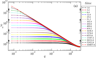
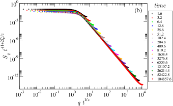
Figure 4: (Color online) Structure factor of the string at different times during evolution at $f=f_{c}$. (a) Raw data. (b) Rescaled data. The parameters $z=1.5$ and $\zeta=1.25$ were used. The curves correspond to a system size $L=M=8192$, and averages were taken over $N=10000$ samples.

In Fig. 4 we show the string averaged structure factor at different times during the evolution of the system in the presence of the applied force $f=f_{c}=1.915$. As can be seen in Fig.4(a), at large length scales (small values of $q$) the system keeps memory of its initial state, which we have chosen to be flat. At small length scales though (but not small enough to explore the lattice effects), the geometry of the string becomes approximately self affine, being characterized by a behavior $S_{q}\sim q^{-(1+2\zeta)}$ where $\zeta$ is the roughness exponent. In Fig.4(b) we test the scaling hypothesis of Eq. (12), by using $z=1.5$ kolton_short_time_exponents and $\zeta=1.25$ duemmer2 ; rosso_roughness_at_depinning .

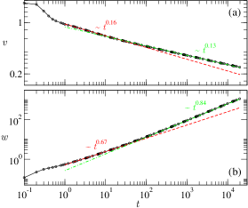
Figure 5: (Color online) Non-stationary velocity (a) and width (b) as functions of time for $f=f_{c}=1.915$. Black dots correspond to data. Dashed red and dot-dashed green curves are power law fits in the regions $1<t<30$ and $30<t<21000$, respectively. The data correspond to $L=M=8192$, and averages were taken over $N=3500$ samples.

As we can observe in Figs. 4(b) and 3(b), the assumed critical exponents $\beta=0.33$, $\nu=1.33$, $\zeta=1.25$, and $z=1.5$ produce rather good collapses. We will argue however that these exponents are effective and have an appreciable bias, which causes the small deviations appreciated in those collapses. This can be perceived only by simulating large systems and reaching several orders of magnitude in time. In Fig. 5 we show $v(t)$ and $w(t)$ vs $t$ at the critical force $f_{c}$. Above the microscopic time regime of order $t_{\tt mic}\sim 1$ we observe in $v(t)$ a crossover at a time $t_{\tt cross}\sim 50$, between two approximate power-law decays with exponents $\approx 0.16$ for short but mesoscopic times, and $\approx 0.13$ for times larger than a few tens [see Fig.5(a)]. A similar crossover is seen in Fig.5(b) where we observe a crossover between two approximate power-law decays, from $\approx 0.67$ to $\approx 0.84$. This behavior is unexpected from the universal non-steady relations $v(t)\sim t^{-\beta/\nu z}$ and $w(t)\sim t^{\zeta/z}$, which generally assume a microscopically very short transient regime before reaching the truly universal macroscopic time regime. In order to understand this behavior, in the next section we analyze this crossover in detail.

IV.3 Robustness of the crossovers

The first question we can ask is how robust are the observed crossovers and in particular, how much they depend on specific details such as the intensity or the shape of the microscopic disorder correlator.

For a given disorder distribution, we have first checked, by simulating $v(t)$ at the corresponding critical force, that the crossover time ($t_{\tt cross}\sim 50$) does not change appreciably by changing the nature of the disorder.

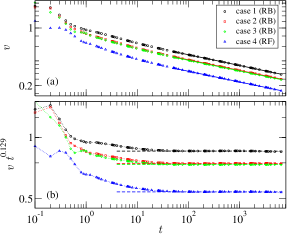
Figure 6: (Color online) Velocity at the corresponding critical forces of the four different cases defined in the text. (a) Raw data. Power-laws fits of the form $v\sim t^{\beta/\nu z}$ for times $t\gtrsim 30$ give similar results for all curves, consistent with $\beta/\nu z=0.129\pm 0.002$. (b) Velocity multiplied by $t^{0.129}$. Dashed horizontal lines showing the apparent scaling regime are displayed to guide the eye. All curves correspond to $L=4096$, $M=8192$, and averages over $N=50000$ samples.

In order to study the dependence of the crossover on the shape and nature of the microscopic disorder correlator, we have fixed $\Delta(0)$, defined in Eq. (2), and analyzed four different cases:

• Case 1: Gaussian-distributed disorder potential with cubic spline interpolation between the integers (RB),

• Case 2: Uniformly-distributed disorder potential with cubic spline interpolation between the integers (RB),

• Case 3: Gaussian-distributed disorder potential with linear spline interpolation between the integers (RB),

• Case 4: Gaussian-distributed random forces (RF) without interpolation between the integers.

Case 1 corresponds to the usual Gaussian-distributed disorder with cubic spline that we used in Sec. IV.2. Case 2 consists in using a uniformly distributed disorder instead of the Gaussian-distributed numbers of the first case. In Case 3 we determine the continous potential using linear interpolation instead of a cubic one, so the pinning force as a function of the position has discontinuities at the integers. These first three cases correspond to random-bond disorder, as the quenched potential fluctuations $\overline{[U(u,x)-U(u^{\prime},x^{\prime})]^{2}}\sim\delta(x-x^{\prime})$ saturate at long distances $|u-u^{\prime}|$. Case 4 is a typical random-field with Gaussian disorder, corresponding to $\overline{[U(u,x)-U(u^{\prime},x^{\prime})]^{2}}\sim\delta(x-x^{\prime})|u-u^{\prime}|$ for large $|u-u^{\prime}|$. Case 4 helps us in particular to answer the question of whether the observed crossovers may be related to the crossover from RF to RB expected for depinning ledoussal_frg_twoloops .

In Fig. 6 we show the time dependent velocity for the four cases, each one at its corresponding thermodynamic critical force, determined with the STD method. Apart from a factor depending on $f_{c}$, the qualitative behavior of $v(t)$ appears unaltered for times longer than some microscopic threshold $t_{\tt mic}\sim 1$. This time is controlled by the microscopic correlator range kolton_short_time_exponents , which is the same in the four cases, $r_{f}=1$. If we fit pure power laws for all curves in the region $t\gtrsim t_{\tt cross}\approx 50$ we find, within the error bars, consistent values for the exponent $\beta/\nu z\sim 0.129$, as shown in Table 1. By plotting $vt^{0.129}$ vs $t$, we clearly see that corrections to scaling at intermediate times ($t_{\tt mic}<t<t_{\tt cross}$) are present. They have an approximate algebraic decay, and seem to have a weak dependence on the microscopic disorder. We thus conclude that the observed value for $\beta/\nu z$ is universal as expected. Moreover, the corrections to scaling appear to be robust: they do not strongly depend on the intensity, shape, or nature (RB vs RF) of the short-ranged correlated microscopic pinning force.

Case	description	$f_{c}$	fitted $\beta/\nu z$
1	RB CS Gaussian	$1.915\pm 0.002$	$0.130\pm 0.001$
2	RB CS Uniform	$1.848\pm 0.002$	$0.128\pm 0.001$
3	RB LS Gaussian	$1.565\pm 0.002$	$0.129\pm 0.001$
4	RF Gaussian	$0.971\pm 0.001$	$0.130\pm 0.001$

Table 1: Critical forces and exponents for four different cases: CS and LS stand for cubic-spline and linear-spline interpolations for the potential, respectively. RB and RF correspond to the random-bond and random-field cases. The power-law fits are consistent with a universal value $\beta/\nu z=0.129\pm 0.001$.

The crossovers in Fig. 6 can be thus possibly ascribed to leading order power-law scaling corrections to the universal non-steady dynamics, similar to what is observed in the Ising, Potts, and $XY$ models for instance luo_corrections ; zheng2_corrections ; zheng_corrections . As is customary, one can try here to fit a “corrected” formula in order to get an unbiased value for ${\beta/\nu z}$:

$$v=v_{0}t^{-\beta/\nu z}\left[1+\left(\frac{t}{t_{0}}\right)^{-\alpha}\right].$$ (16)

However, with the present data, we find that this procedure is inaccurate as it involves several parameters introduced through an ad hoc formula for the correction.

This takes us to our next step, the search for a different practical criterion to directly estimate $t_{\tt cross}$. We start by observing that in the truly universal non-steady macroscopic critical regime, the quantity

$$\gamma(t)=\frac{w(t)}{tv(t)}$$ (17)

should reach a time-independent constant value as a consequence of the scaling relation $\beta=\nu(z-\zeta)$: since at $f=f_{c}$ in the macroscopic regime, $v(t)\sim t^{-\beta/\nu z}$ and $w(t)\sim t^{\zeta/z}$, then $\gamma(t)\sim\mathrm{const}$. This criterion was used to determine the depinning threshold in the long-range discrete elastic model olaf_std_longrangedepinning , since any departure from $f_{c}$ would make $\gamma$ vanish, or increase with time at very long times. For our present purposes, we note that if the measured $\gamma(t)$ depends on time, it means that we have not reached the critical scaling regime yet. Therefore, a constant $\gamma(t)$ is, at least, a necessary condition.

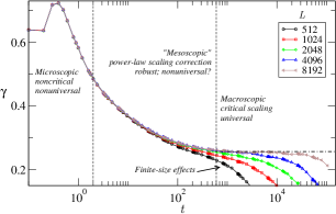
Figure 7: (Color online) $\gamma(t)$ as a function of time for Case 1 and different system sizes at $f=f_{c}=1.915$. The vertical dashed lines separate qualitatively the different dynamical regimes observed. The curves correspond to $M=32768$, the averages were taken over $N=5000$ samples for $L=512,1024,2048$, $N=3000$ samples for $L=4096$, and $N=1700$ samples for $L=8192$.

In Fig. 7 we show the behavior of $\gamma(t)$ with time for Case 1. After a microscopic regime we can see a decreasing behavior of $\gamma(t)$ with time, which implies an “effective” unbalanced relation $\left[\nu(z-\zeta)-\beta\right]_{\mathrm{eff}}<0$. The system is then in what we call a “mesoscopic” regime where the critical dynamics scaling [Eq. (8)] is still not valid. Nevertheless, it is possible to fit a reasonable power law for $v(t)$ in this regime, if larger times are not available. We hence see the importance of having a good criterion to decide where to fit the exponents: if the time is not large enough, the resulting exponents will be effective and have a systematic bias. Moreover, using $\gamma(t)$ as a method to determine $f_{c}$ may also suffer from these mesoscopic time effects, as its initial decay may be incorrectly ascribed to having an applied force larger than $f_{c}$. After that long crossover, we can observe that $\gamma(t)$ develops a plateau starting at $t\sim 1000$. This plateau is cut-off by finite-size effects, which introduce an $L$-dependent characteristic time. We also observe that scaling corrections in $v(t)$ or $w(t)$, shown in Figs. 5 and 6, are important in the mesoscopic time regime, clearly visible in the time-dependence of $\gamma(t)$. We thus argue that within the plateau in $\gamma(t)$, scaling corrections are already negligible, and the true critical exponents can be consistently extracted with the STD method. As we see in Fig. 7, this criterion is strongly limited by finite size effects, reducing the time range of the plateau. We observe that in order to obtain a sufficiently wide time window to fit the exponents accurately (i.e., a few decades in time), we really need to attain big system sizes, much larger than $L=8192$.

IV.4 Large-scale simulations

With the numerical method implemented so far, in periodic samples of size $L\times M$, we are limited  to system sizes not much bigger than $L=8192$. This is because we need sufficiently large $M$ in order to avoid undesirable periodicity effects, i.e., a crossover to the random-periodic class bustingorry_paperinphysics . We hence move to our “memory-free” numerical implementation, where we dynamically generate the underlying disorder instead of reading it from a previously stored array, similarly to what was done in Ref. chen_marchetti but with concurrent computations. As we explain in the Supplemental Material supplementalmaterial , in this implementation it is simpler to work with linear splines for interpolating the potential, therefore corresponding to Cases 3 (RB) and 4 (RF) of Sec. IV.3, for which we have already shown that scaling corrections are present.

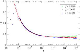
Figure 8: (Color online) $\gamma(t)$ as a function of time for the RB case with Gaussian distributed disorder. The system size is $L=2^{25}=33554432$. The continuous line is a fit using Eq. (18).

In Fig. 8 we present the behavior of $\gamma(t)$ with time for a string of size $L=2^{25}=33554432$, for Case 3. Simulating such large systems give us the benefit of the self-averaging of the velocity. Indeed, in Fig. 8 the smooth curve for $f_{c}$ was averaged only over five samples, while the other two correspond to only one sample. Second, notice that, compared with Table 1, we are now able to improve the determination of the thermodynamical critical force with the STD method, pushing the uncertainty to the fourth decimal place, $f_{c}=1.5652\pm 0.0003$ for Case 3. At this value of $f_{c}$ we obtain a well defined plateau in $\gamma$, lasting approximately two decades, starting at $t\sim 1000$. Ignoring the microscopic time regime $t<t_{\tt mic}\sim 1$, we can now perform a good fit of the data at $f=f_{c}$ with the expression

$$\gamma(t)=G_{0}\left[1+\left(\frac{t}{t_{g}}\right)^{-\alpha_{g}}\right].$$ (18)

Here we have introduced the fitting parameters $G_{0}$, $t_{g}$ and $\alpha_{g}$, obtaining $G_{0}\simeq 1.143$, $t_{g}\simeq 0.142$, and $\alpha_{g}\simeq 0.56$. This allows us to quantify the development of the plateau, and to confirm the power-law shape of the scaling correction in $\gamma(t)$. We are now prepared to consistently fit both the scaling corrections in $w(t)$ and $v(t)$ and the combination of critical exponents $\zeta/z$ and $\beta/\nu z$ respectively.

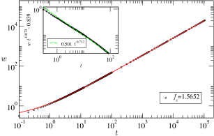
Figure 9: (Color online) String width $w(t)$ as a function of time for the RB case with Gaussian-distributed disorder. The system size is $L=2^{25}=33554432$.

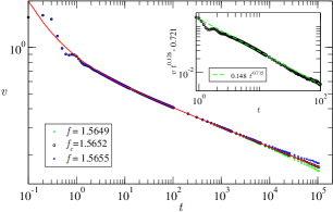
Figure 10: (Color online) String velocity $v(t)$ as a function of time for the RB case with Gaussian-distributed disorder. The system size is $L=2^{25}=33554432$.

In Figs. 9 and 10 we show $w(t)$ and the velocity $v(t)$ as functions of time, for $L=2^{25}=33554432$ and for an applied force $f_{c}=1.5652$, corresponding to a RB linearly interpolated random-potential generated with Gaussian numbers. In Fig. 10, we have also included the behavior of the string for two other forces, just above ($f=1.5655$) and just below ($f=1.5649$) the estimated depinning force $f_{c}$. For $w(t)$ the corresponding three curves are indistinguishable, so we show only the curve corresponding to $f=f_{c}$. We can see very nice asymptotic power-law behaviors of both quantities, spanning several orders of magnitude. Nevertheless, as noticed for $\gamma(t)$ in Fig.8, a proper power-law fit can be accomplished only after deciding a starting point for the scaling regime. With the criterion of a plateau in $\gamma(t)$ such a starting point could be decided up to some arbitrariness, but it can be included in the final uncertainty of the fitted exponents. In addition, we propose corrected expressions for $w$ and $v$ that can be used to fit the data during all the non-steady evolution, excluding the microscopic regime $0\leq t<t_{\tt mic}\sim 1$. The corrections to scaling in these quantities then read

$$w(t)=W_{0}~{}t^{\zeta/z}\left[1+\left(\frac{t}{t_{w}}\right)^{-\alpha_{w}}\right],$$ (19)

$$v(t)=V_{0}~{}t^{-\beta/\nu z}\left[1+\left(\frac{t}{t_{v}}\right)^{-\alpha_{v}}\right].$$ (20)

The fits give $W_{0}\simeq 0.839$, $t_{w}\simeq 0.485$, and $\alpha_{w}\simeq 0.712$ for the width, and $V_{0}\simeq 0.721$, $t_{v}\simeq 0.110$, and $\alpha_{v}\simeq 0.715$ for the velocity. The insets of Figs. 9 and 10 confirm that the corrections can be fairly described by power-laws, as observed earlier in Sec. IV.3 for smaller systems. The fitted parameters are to some extent sensitive to the choice of $t_{\tt mic}$ but this arbitrariness can be included in the error bars, and the proposed form of the corrected critical behavior is robust.

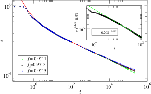
Figure 11: (Color online) String velocity $v(t)$ as a function of time for the RF case with Gaussian-distributed disorder. The system size is $L=2^{25}=33554432$.

For completeness, we also present the corrections to scaling for the RF case. In Fig. 11 we can see the behavior of the string velocity with time when we apply the critical force for the RF case $f_{c}=0.9713\pm 0.0002$ and different forces close to $f_{c}$. The complete picture of the RB case is repeated, but now the expression Eq. (20) gives back slightly different exponents for the corrections to scaling. The fit gives $V_{0}\simeq 0.53$, $t_{v}\simeq 0.382$ and $\alpha_{v}\simeq 0.927$ in this case. Nevertheless we cannot confirm whether or not the correction exponents are distinguishable between the RB and RF cases, since they are very sensitive to the choice of the arbitrary quantity $t_{\tt mic}$, the time from which we start the fitting. For example for the RF case $\alpha_{v}$ changes between $0.69$ and $0.99$ when $t_{\tt mic}$ is varied from $2$ to $10$.

However, for the RF case we find a $\beta/\nu z$ which is indistinguishable from the one extracted for the RB case, as detailed in the following section. With the precision we have, we can not rule out, however, that these exponents are actually the same for the RB and RF cases, and thus maybe universal.

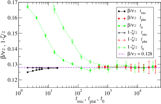
Figure 12: (Color online) The combination of exponents $1-\zeta/z$ and $\beta/\nu z$ extracted from fittings to the data of Figs. 9 and 10, respectively. The horizontal axes shows the chosen values of three different arbitrary quantities for the fitting procedure. In black (full lines) we show the time $t_{\tt mic}$ on and after which we fitted using the corrected expressions (19) and (20). In red (dotted lines) is shown the time $t_{\tt plat}$ from which we can consider $\gamma(t)$ to be constant, and we fitted $w(t)$ and $v(t)$ with pure power laws $v\sim t^{-\beta/\nu z}$ and $w\sim t^{\zeta/z}$, without corrections. In green (dot-dashed lines) we show the exponents as a function of $t_{0}$, with $t_{0}$ such that we fitted the data with pure power laws in the window $[t_{0},4t_{0}]$.

IV.5 Critical exponents

We are now in position to accurately and consistently determine the critical exponents $\beta$ and $z$ from the non-stationary dynamical behavior of the system. In Fig. 12 we show our determination of $\beta/\nu z$ and $\zeta/z$ [presented as $(1-\zeta/z)$ since these are expected to be equal] extracted from $v(t)$ and $w(t)$, respectively. To check the consistency of the fitted values we have used three different fitting procedures:

• First, as is customary, we use the corrected expressions (19) and (20) to extract $(\zeta/z)$ and $(\beta/\nu z)$, respectively. The fit should be performed above the microscopic regime $t>t_{\tt mic}$. Since the microscopic time $t_{\tt mic}$ is not precisely defined we let it vary in a reasonable range $t\in[2,20]$ and compare the values fitted for $(\zeta/z)$ and $(\beta/\nu z)$ according to (19) and (20).

• Second, we use the “plateau in $\gamma$” criterion to fit our exponents. That is, we first observe the behavior of $\gamma(t)$, and propose a time $t_{\tt plat}$, above which we can consider the plateau well developed. From $t>t_{\tt plat}$ we fit separately $w(t)$ and $v(t)$ with the pure power-law expressions $w=w_{0}t^{\zeta/z}$ and $v=v_{0}t^{-\beta/\nu z}$, respectively. Again, since $t_{\tt plat}$ is not precisely defined, we allow it to move in a wide window $t_{\tt plat}\in[500,40000]$ and observe how the fitted exponents $(\zeta/z)$ and $(\beta/\nu z)$ behave.

• Third, we perform pure power-law fittings of our data, as in the previous case, but now we perform fits within time windows $t\in[t_{0},4t_{0}]$ where $t_{0}$ is arbitrarily chosen in a wide range of values. This is to show how the resulting exponent changes depending on the selected time window and to mimic the situation where long-time runs of large systems are not available.

Figure 12 shows that the three fitting procedures lead to the same result $\beta/\nu z\approx 1-\zeta/z\approx 0.128$, for sufficiently large $t_{\tt mic}$, $t_{\tt plat}$ and $t_{0}$. Interestingly, the values fitted for $1-\zeta/z$ and $\beta/\nu z$ in the third procedure are very sensitive to $t_{0}$, and show a clear tendency to produce a positive bias on both at small times. This explains the previous observations of larger effective values for $(\beta/\nu z)$ kolton_short_time_exponents . On increasing $t_{0}$, while keeping the window selection as $[t_{0},4t_{0}]$ (other choices different from the factor $4$ give the same qualitative result), the exponent values decrease and at some point the dependence on $t_{0}$ ceases. This coincides with the beginning of the range of good values for $t_{\tt plat}\sim 1000$. From this analysis we conclude for the depinning transition of the QEW elastic line, that

$$\beta/(\nu z)=1-\zeta/z=0.128\pm 0.003.$$ (21)

Combining this with the value of $\zeta=1.250\pm 0.005$, obtained in Sec. IV.1 with a reliable exact steady-state method, this finally gives

$$z=1.433\pm 0.007;$$ (22)

and considering the statistical tilt symmetry of the model, which yields $\nu=1/(2-\zeta)$, we obtain

$$\nu=1.333\pm 0.007$$ (23)

and

$$\beta=0.245\pm 0.006.$$ (24)

IV.6 Scaling relations around the critical point

Now that we know the accurate critical exponents of the model, we test them in large scale simulations around the critical point, i.e., at force values around the critical force $f_{c}$.

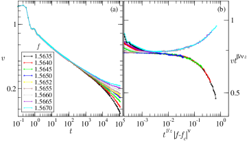
Figure 13: (Color online) String velocity $v(t)$ as a function of time for the RB case with uniformly distributed disorder for which $f_{c}=1.5652$ using $\delta t=0.1$. The system size is $L=4194304$. In (a) we present the raw data, and in (b) $v(t,f)$ has been rescaled to $vt^{\beta/\nu z}$ and $t$ to $t^{1/z}|f-f_{c}|^{\nu}$.

In Fig. 13(a) we present the behavior of $v(t)$ with time, at different driving forces, for a string of size $L=2^{22}=4194304$. In Fig. 13(b) we scale the data according to Eq. (15) with the exponents just obtained. Compared with Fig. 3 for a much smaller system, we now get a much better scaling, especially for large times, and since we are using now the new set of critical exponents.

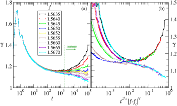
Figure 14: (Color online) $\gamma(t)$ as a function of time for the RB case with uniformly distributed disorder for which $f_{c}=1.5652$ using $\delta t=0.1$. The system size is $L=4194304$. In (a) we present the raw data, and in (b) $t$ has been rescaled.

Consistently, Fig. 14(a) we show that the quality of the collapse in Fig. 13(b) is closely accompanied by the development of a plateau in $\gamma(t)$ with time at $f\approx f_{c}$, for $t\gtrsim 1000$. For forces greater or smaller than $f_{c}$, $\gamma$ deviates from its flat behavior towards decreasing or increasing, respectively. Using the facts that in the scaling region we expect $v(t,f)\sim t^{-\beta/\nu z}G_{v}(|f-f_{c}|^{\nu}t^{1/z})$ and $w(t,f)\sim t^{\zeta/z}G_{w}(|f-f_{c}|^{\nu}t^{1/z})$, with $G_{v}(x)$ and $G_{w}(x)$ some universal functions we get $\gamma(t,f)\sim F(|f-f_{c}|^{\nu}t^{1/z})$, with a new universal function $F(y)$. This scaling is checked in Fig. 14(b) and, again, the quality of the collapse is closely accompanied by the development of a plateau in $\gamma(t)$ at $f\approx f_{c}$, occurring for $t\gtrsim 1000$. This shows that our criterion for bounding the scaling region is consistent.

V Discussion

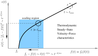
Figure 15: (Color online) Heuristic connection between steady state and the non-steady universal relaxation at the thermodynamical critical force $f_{c}$. The circle represents the system and the short arrows indicate its non-steady time evolution. At large times, in the critical region, we can think of the relaxation of the velocity as “driven” by the small finite-size bias of the critical force $f_{c}-f_{c}(\ell)\sim\ell^{-1/\nu}$ at the scale $\ell=\ell(t)\sim t^{1/z}$, where $f_{c}$ is the thermodynamic value. Although the geometry of the interface beyond $\ell(t)$ still retains memory of the initial condition, these large-wavelength modes will not affect $v(t)$.

Power-law corrections to the non-equilibrium scaling have been observed in several other systems such as Ising, Potts, and $XY$ models  luo_corrections ; zheng2_corrections ; zheng_corrections . Interestingly, it is found that these corrections are stronger for systems with disorder or frustration, or dilution review_albano . Corrections are usually used to improve the accuracy of the exponents obtained by the STD method. For the depinning transition we have shown that this practice does not much increase the accuracy of the STD method. We think that one reason is that we rely on an ad hoc model for the corrections, add extra parameters to the fit, and still have to decide where to start fitting the corrected formula (the non-universal microscopic time). We have shown that a better approach for depinning is to use scaling relations between the exponents that are violated in the presence of corrections. This allows us to find the truly assymptotic regime where we can expect to get very close to the true exponents. We think it may be useful to try this kind of approach in other problems.

A heuristic explanation for the power-law corrections can be proposed by relating Eq. (11) to the steady-state relation $v\sim\xi^{-\beta/\nu}$. As we already pointed out, replacing $\xi$ by the correlation length $\ell(t)\sim t^{1/z}$ yields Eq. (11), obtained from general arguments. This suggests two simple pictures: (i) In the first picture we simply introduce phenomenological corrections to the dynamical exponent as $\ell^{\prime}(t)\sim t^{1/z}(1+|c_{3}|t^{-\epsilon})$ with $c_{3}$ and $\epsilon$ parameters of the correction. This type of correction has been introduced in studies of the off-equilibrium critical dynamics of the three-dimensional diluted Ising model, for instance, and attributed to the biggest irrelevant eigenvalue of the renormalization group in the dynamics parisi_corrections . If we assume that $v(t)\sim\ell^{\prime}(t)^{-\beta/\nu}$ holds, it is easy to see that such a correction would lead to a corrected velocity $v(t)\sim t^{-\beta/z\nu}(1+|c_{2}|t^{-\sigma})$ with parameters $c_{2}$ and $\sigma$. Something similar would happen with $w(t)$. Note, however, that if $w(t)\sim\ell^{\prime}(t)^{\zeta}$ also held, we would not explain the corrections observed, in the same time regime, in $\gamma(t)=w(t)/v(t)t$. In any case, it would be interesting to see whether such corrections for $\ell(t)$, which are certainly absent in the non-steady relaxation of a flat line in the EW model at $T>0$ for instance (and more generally of non-Markovian Gaussian signals santachiara_gaussian_signals ; rosso_gaussian_signals related to manifolds with long-range elasticity), can be explained using the complicated coupling between Fourier modes induced by the non-linearity of the quenched disorder. It is known that “non-Gaussian” effects are indeed subtle rosso_width_distribution ; rambeau_maximums . (ii) In the second picture we assume that the universal non-steady relaxation at the thermodynamic threshold $f_{c}$ is actually “quasistatically driven” by the finite-size bias of the critical force. In other words, the small velocity of the large string is roughly controlled by the steady-state dynamics of an effective string of increasing size $\ell(t)$ and width $w(t)\sim\ell(t)^{\zeta}$, as $v(t)\sim[f_{c}-f_{c}(\ell(t))]^{\beta}$. Indeed, if we assume that this finite-size bias with respect to the thermodynamic value $f_{c}$ is positive, and scales with $\ell$ exactly as the finite-size critical force fluctuations around its mean value, i.e., $f_{c}-f_{c}(L)\sim L^{-1/\nu}$, we get

$$v(t)\sim[f_{c}-f_{c}(\ell(t))]^{\beta}\sim\ell(t)^{-\beta/\nu}\sim t^{-\beta/\nu z},$$ (25)

equivalent to Eq. (11). This picture is schematized in Fig. 15. The assumption of a positive bias $f_{c}-f_{c}(L)\sim L^{-1/\nu}$ can be justified from results using the quasi-statically velocity-driven ensemble, where the interface is driven by a parabolic potential $m^{2}(vt-u)$. For small $m$, it was shown, via the functional renormalization group (FRG), that $f_{c}(m)=f_{c}-|c_{1}|m^{2-\zeta}=f_{c}-|c_{1}|m^{1/\nu}$, with $c_{1}$ a constant rosso_correlator_RB_RF_depinning . Since the parabola imposes a characteristic length $L_{m}\sim m^{-1}$, beyond which the driven interface looks flat, we can write $[f_{c}-f_{c}(m)]\sim L_{m}^{-1/\nu}$. Identifying $L_{m}$ with $\ell(t)$, we explain the assumed positive bias and again get Eq. (11). This identification of lengths is supported by the fact that both $L_{m}$ and $\ell(t)$ (for the initially flat line) represent the same geometrical crossover. For lengths below $\ell(t)$(or $L_{m}$), the string is steady-state quasi-equilibrated with the pinning landscape yielding the roughness exponent $\zeta$, but it remains macroscopically flat because of the memory of the initial condition (due to the confinement of the parabola) at scales above $\ell(t)$ (or $L_{m}$). With the picture above we can now speculate about a possible mechanism for generating the scaling correction. Since the formula $f_{c}(\ell)=f_{c}-|c_{1}|\ell^{-1/\nu}$ is expected to hold only in the limit of large $\ell$ it is plausible to add corrections to it, which decay to zero in the large $\ell$ limit. If we add a correction of the type $f_{c}(\ell)=f_{c}-|c_{1}|\ell^{-1/\nu}(1+|c_{2}|\ell^{-\alpha})$ with $\alpha>0$ and $c_{2}$ constants, and use $v(\ell)\sim[f_{c}-f_{c}(\ell)]^{\beta}$, we get $v(t)\sim t^{-\beta/z\nu}(1+|c_{2}|t^{\alpha/z})$, using $\ell=\ell(t)=t^{1/z}$, the same type of correction we observe in our simulations. The correction just proposed is not completely ad hoc, but qualitatively consistent (the same sign and order of magnitude) with the corrections to the FRG formula $f_{c}(m)=f_{c}-|c_{1}|m^{2-\zeta}$ observed at intermediate values of $m$ in simulations in the quasistatically velocity-driven ensemble rosso_correlator_RB_RF_depinning . It would thus be interesting, in the first place, to check quantitatively whether such corrections are directly related to the ones we report here, and in the second place to check whether one can explain them directly from the FRG-flow behavior. This picture for the corrections suggests that both finite-size steady-state simulations and finite-time non-steady simulations would yield, in particular, an effective exponent for $\beta$ larger than the true one. This may explain the trend of discrepancies found in the literature. In any case, an analytical and more fundamental description of these effects would be welcomed.

exponent	estimate	reference
$\zeta$	$0.97\pm 0.05$	chen_marchetti
	$1.25\pm 0.05$	leschhorn_automaton
	$1.25\pm 0.01$	tang_unpublished
	$1.2\pm 0.2$	ledoussal_frg_twoloops
	$1.26\pm 0.01$	rosso_roughness_at_depinning
	$1.250\pm 0.005$	this work
$z$	$1.42\pm 0.04$	leschhorn_automaton
	$1.54\pm 0.05$	tang_unpublished
	$1.35\pm 0.2$	ledoussal_frg_twoloops
	$1.433\pm 0.007$	this work
$\nu$	$1.05\pm 0.1$	chen_marchetti
	$1.00\pm 0.05$	nowak_thermal_rounding
	$1.1\pm 0.1$	tang_unpublished
	$1.25\pm 0.3$	ledoussal_frg_twoloops
	$1.29\pm 0.05$	duemmer2
	$1.33\pm 0.01$	bolech_critical_force_distribution
	$1.333\pm 0.007$	this work
$\beta$	$0.25\pm 0.03$	nattermann_stepanow_depinning
	$0.24\pm 0.01$	chen_marchetti
	$0.34\pm 0.04$	nowak_thermal_rounding
	$0.40\pm 0.05$	tang_unpublished
	$0.25\pm 0.03$	leschhorn_automaton
	$0.22\pm 0.02$	lacombe_1d_elastic_chain
	$0.2\pm 0.2$	ledoussal_frg_twoloops
	$0.33\pm 0.02$	duemmer2
	$0.245\pm 0.006$	this work

Table 2: Representative values for the depinning exponent $\zeta$, the dynamical exponent $z$, and the critical exponents $\nu$ and $\beta$, reported in the literature. The major dispersion is seen in the value of $\beta$.

The critical exponents associated with the depinning transition for the QEW model in one dimension as reported in previous works are shown in Table 2, together with the values obtained in the present work. Comparing previous estimates, the largest discrepancy is found for the $\beta$ exponent. Our value $\beta=0.245\pm 0.006$ is more precise than previous reported values and agrees well with the ones obtained in automaton models leschhorn_automaton and in molecular dynamics simulations chen_marchetti , but disagrees appreciably with respect to random-field Ising model simulations nowak_thermal_rounding and other molecular dynamics simulations duemmer2 , which give about $30\%$ larger values. All these works correspond to the steady-state dynamics. They thus rely on a proper steady-state equilibration and on a precise knowledge of the critical threshold, which is difficult to achieve, except in periodic samples rosso_dep_exponent ; duemmer2 . In steady-state simulations with dynamically generated disorder, such as the ones in Ref. chen_marchetti , one should be cautious at long times or large center of mass displacements, because of the critical force extreme statistics, since, in this case, $f_{c}$ can be considered as the maximum among $\sim M/L^{\zeta}$ independent typical critical forces bolech_critical_force_distribution ; fedorenko_frg_fc_fluctuations ; ledoussal_driven_particle . Therefore, a finite-velocity steady-state might not exist at zero temperature if the critical force statistics tends to Gumbel’s type for large $M/L^{\zeta}$ for instance, as the interface will eventually be blocked (by virtue of the Middleton theorems middleton_theorem ) at any finite-force. It is not clear how a finite temperature can diminish the dominant effect of these rare events at very large averaging times, or eliminate the sensibility to the tails of the distributions. At $T=0$, one possibility is to perform a disorder average over finite time averages of the steady-state velocity, such that the distance covered by the center of mass is of order $L^{\zeta}$, and thus the critical force becomes typical again. The problem with this approach is that this critical force fluctuates and thus the control parameter $f-f_{c}$ also varies from sample to sample, complicating the direct estimation of $\beta$. In this respect finite samples with periodic disorder have the great advantage that we can calculate accurately the critical force for each sample using an exact algorithm rosso_dep_exponent . Steady-state simulations exploiting this algorithm were limited by the narrow scaling region for obtaining $\beta$ duemmer2 however, bounded by finite-size effects on one side, and by the effects of the crossover to the Edwards-Wilkinson equation at large velocities on the other side. Additionally, one should also be cautious with periodic boundary conditions: if $M$ is small compared to the expected random-manifold width, i.e., $M\ll L^{\zeta}$, we can have several crossovers from the random-manifold to the random-periodic universality class. In this respect one should be warned that, for a fixed $L$, the crossovers to the random-periodic class are not controlled only by $M$, but also by the velocity bustingorry_periodic ; bustingorry_paperinphysics .

The STD method applied to the depinning transition has the advantage, on one hand, that it does not suffer from finite-size effects, as it assumes a growing correlation length which should lie well below the system size. On the other hand, it does not suffer from extreme statistics either, as the spatial region covered in the scaling region is at maximun of order $L^{\zeta}$ and thus the critical force and configuration can not be rare. Moreover, we have shown that it actually detects the thermodynamical critical force corresponding to the random-manifold family $M=kL^{\zeta}$, separating the random-periodic case for $k\to 0$, and the extreme Gumbel case $k\to\infty$ bolech_critical_force_distribution . We have shown, however, that in order to have a long power-law decay in $v(t)$ we must use a large system with the force precisely tuned to the thermodynamic critical force $f_{c}$. Fortunately, as shown in Fig.2, $f_{c}$ can be unambiguously and precisely determined from a finite-size analysis of the precisely known sample critical force $f_{c}^{s}$ of periodic samples. It is also usually said that the STD method has the advantage that we do not need to (steady-state) equilibrate the system. The presence of power-law-like scaling corrections shows, however, that we do need to wait (or correct) until the truly asymptotic universal non-steady regime is reached, before determining the exponents. It is also worth noting that the STD method does not yield $\beta$ or $\zeta$ directly, as the direct steady-state method does, but the combination of exponents $\beta/\nu z$. This is not very problematic however, since for the QEW model we accurately determine $\zeta$ from the analysis of large critical configurations rosso_roughness_at_depinning , $\nu=1/(2-\zeta)$, from the statistical tilt-symmetry exact relation, and $\zeta/z$, from the power-law increase of the width $w(t)$, as shown in Fig. 9. It would thus be interesting to try the STD method in the computationally more convenient automaton models belonging to the QEW universality class. Such models are described in pioneering papers such as Ref. leschhorn_automaton . Since by construction they involve a kind of coarse-grained dynamics, it would be instructive to study the non-steady dynamics of this model and see what happens in the mesoscopic time-regime reported here.

VI Conclusions

We have studied the non-steady relaxation of a driven one-dimensional elastic interface at the depinning transition. Above a first, non-universal microscopic time regime, we have found a non-trivial long crossover towards the non-steady macroscopic critical regime, expected from general scaling arguments. We have shown that this mesoscopic time regime is robust under changes of the microscopic disorder, including its random-bond or random-field character, and can be fairly described as power-law corrections to the asymptotic scaling forms yielding the true critical exponents. These corrections may explain some numerical discrepancies found in the literature (as large as $30\%$ for some exponents), for this universality class. In particular they explain the appearance of effective power laws in the nonsteady relaxation with exponents presenting a systematic bias with respect to the critical values. To improve the accuracy and consistency of the STD method for extracting critical exponents, we have implemented a practical criterion of consistency and tested it in large-scale ($L=2^{25}$) simulations concurrently implemented on GPUs. In this way we obtained accurate exponents for the universality class of the paradigmatic continuum displacement quenched Edwards-Wilkinson equation. Accurate critical exponents are necessary tu succeed in classifying diverse experimental systems and theoretical models into universality classes. It is interesting to note that our estimates coincide, within error bars, with the critical exponents obtained for a stochastic sandpile model in the conserved directed-percolation class bonachela The method applied in the present paper may be used to analyze exponents in different depinning universality classes, such as the long-range elasticity, quenched Kardar-Parisi-Zhang, or correlated disorder classes fedorenko_longrange_correlated_disorder .

We believe that the features here observed might be experimentally relevant. In many experiments at low temperatures with magnetic or electric domain walls, or with contact lines of liquids, the dynamics of the interface is non-stationary, in the sense that the system keeps for a while a memory of the initial conditions (i.e. the memory of the preparation or “writing” of the domain wall is visible in the experimental time and length scales), and a growing dynamical correlation length is slowly developed in the presence of a driving field. The STD method might be thus applied experimentally to determine the critical field and exponents, and ultimately to determine the universality class of the system. In particular, we have shown here that scaling corrections are important in a mesoscopic time regime, between the so-called microscopic and macroscopic time-regimes. It would be important to determine whether this regime can be accessed experimentally. In this respect we note that in systems with weak pinning, where the microscopic time-regime $t<t_{\tt mic}$ is determined by a large Larkin length $\ell_{c}$, we have $\ell(t_{\tt mic})\sim t_{\tt mic}^{1/2}\sim\ell_{c}$ kolton_short_time_exponents . If $t_{\tt mic}$ is large enough, the mesoscopic time-regime might be observable. In such cases, our criterion of consistency may be useful, as we only require monitoring of the time dependence of the interface width and velocity simultaneously (by direct imaging for instance). This would allow corrections from the truly universal part of the relaxation to be disentangled and accurate critical steady-state exponents to be obtained experimentally. Finally, the inclusion of thermal fluctuations would be important in order to compare with some experiments. If the temperature is small enough, we expect a critical universal relaxation yielding the zero-temperature depinning exponents up to length-scales comparable with the thermal rounding length $\xi_{T}\sim T^{-\psi\nu/\beta}$ or up to time-scales of the order of $\xi_{T}^{z}$. The STD method can thus also be used to determine $\psi$ bustingorry_thermal_depinning_exponent .

- (1) M. Kardar, Phys. Rep. 301, 85 (1998)
- (2) D. S. Fisher, Phys. Rep. 301, 113 (1998)
- (3) D. S. Fisher, Phys. Rev. Lett. 56, 1964 (1986)
- (4) P. Chauve, T. Giamarchi, and P. Le Doussal, Phys. Rev. B 62, 6241 (2000)
- (5) P. Le Doussal, K. J. Wiese, and P. Chauve, Phys. Rev. B 66, 174201 (2002)
- (6) D. A. Huse and C. L. Henley, Phys. Rev. Lett. 54, 2708 (Jun 1985), http://link.aps.org/doi/10.1103/PhysRevLett.54.2708
- (7) M. Kardar, Phys. Rev. Lett. 55, 2923 (Dec 1985), http://link.aps.org/doi/10.1103/PhysRevLett.55.2923
- (8) H. Leschhorn, Physica A 195, 324 (1993), ISSN 0378-4371,
- (9) A. Rosso and W. Krauth, Phys. Rev. B 65, 012202 (2001)
- (10) A. Rosso and W. Krauth, Phys. Rev. Lett. 87, 187002 (2001)
- (11) A. Rosso and W. Krauth, Phys. Rev. E 65, 025101 (Jan 2002)
- (12) O. Duemmer and W. Krauth, J. Stat. Mech.: Theory. Exp. 2007, P01019 (2007),
- (13) A. B. Kolton, A. Rosso, T. Giamarchi, and W. Krauth, Phys. Rev. Lett. 97, 057001 (2006)
- (14) A. B. Kolton, A. Rosso, T. Giamarchi, and W. Krauth, Phys. Rev. B 79, 184207 (2009)
- (15) S. Lemerle, J. Ferré, C. Chappert, V. Mathet, T. Giamarchi, and P. Le Doussal, Phys. Rev. Lett. 80, 849 (1998)
- (16) M. Bauer, A. Mougin, J. P. Jamet, V. Repain, J. Ferré, R. L. Stamps, H. Bernas, and C. Chappert, Phys. Rev. Lett. 94, 207211 (2005)
- (17) M. Yamanouchi, D. Chiba, F. Matsukura, T. Dietl, and H. Ohno, Phys. Rev. Lett. 96, 096601 (2006)
- (18) P. J. Metaxas, J. P. Jamet, A. Mougin, M. Cormier, J. Ferré, V. Baltz, B. Rodmacq, B. Dieny, and R. L. Stamps, Phys. Rev. Lett. 99, 217208 (2007)
- (19) P. Paruch, T. Giamarchi, and J. M. Triscone, Phys. Rev. Lett. 94, 197601 (2005)
- (20) P. Paruch and J. M. Triscone, Appl. Phys. Lett. 88, 162907 (2006)
- (21) P. Paruch, A. B. Kolton, X. Hong, C. H. Ahn, and T. Giamarchi, Phys. Rev. B 85, 214115 (Jun 2012), http://link.aps.org/doi/10.1103/PhysRevB.85.214115
- (22) J. Guyonnet, E. Agoritsas, S. Bustingorry, T. Giamarchi, and P. Paruch, Phys. Rev. Lett. 109, 147601 (Oct 2012), http://link.aps.org/doi/10.1103/PhysRevLett.109.147601
- (23) S. Moulinet, A. Rosso, W. Krauth, and E. Rolley, Phys. Rev. E 69, 035103(R) (2004)
- (24) P. Le Doussal, K. J. Wiese, S. Moulinet , and E. Rolley, EPL 87, 56001 (2009), http://dx.doi.org/10.1209/0295-5075/87/56001
- (25) E. Bouchaud, J. P. Bouchaud, D. S. Fisher, S. Ramanathan, and J. R. Rice, J. Mech. Phys. Solids 50, 1703 (2002)
- (26) M. Alava, P. K. V. V. Nukalaz, and S. Zapperi, Adv. Phys. 55, 349 (2006)
- (27) E. A. Jagla and A. B. Kolton, J. Geophys. Res. 115, B05312 (2010)
- (28) A. A. Middleton, Phys. Rev. Lett. 68, 670 (1992)
- (29) A. Rosso, A. K. Hartmann, and W. Krauth, Phys. Rev. E 67, 021602 (Feb 2003)
- (30) D. S. Fisher, Phys. Rev. B 31, 1396 (1985)
- (31) O. Narayan and D. S. Fisher, Phys. Rev. B 46, 11520 (1992)
- (32) T. Nattermann, S. Stepanow, L. H. Tang, and H. Leschhorn, J. Phys. II France 2, 1483 (1992)
- (33) L. B. Ioffe and V. M. Vinokur, J. Phys. C 20, 6149 (1987)
- (34) V. M. Vinokur, M. C. Marchetti, and L.-W. Chen, Phys. Rev. Lett. 77, 1845 (Aug 1996), http://link.aps.org/doi/10.1103/PhysRevLett.77.1845
- (35) A. B. Kolton, A. Rosso, and T. Giamarchi, Phys. Rev. Lett. 94, 047002 (2005)
- (36) L. W. Chen and M. C. Marchetti, Phys. Rev. B 51, 6296 (1995)
- (37) U. Nowak and K. D. Usadel, Europhys. Lett. 44, 634 (1998)
- (38) S. Bustingorry, A. B. Kolton, and T. Giamarchi, EPL 81, 26005 (2008)
- (39) S. Bustingorry, A. B. Kolton, and T. Giamarchi, Phys. Rev. E 85, 021144 (2012)
- (40) S. Bustingorry, A. B. Kolton, and T. Giamarchi, Phys. Rev. B 85, 214416 (2012)
- (41) L. F. Cugliandolo, “in Dynamics of Glassy Systems in Slow Relaxation and Nonequilibrium Dynamics in Condensed Matter,” edited by J. L. Barrat et al. (Springer-Verlag, Berlin, 2002) Chap. Course 7, 367-521
- (42) A. B. Kolton, G. Schehr, and P. Le Doussal, Phys. Rev. Lett. 103, 160602 (2009)
- (43) A. B. Kolton, A. Rosso, E. V. Albano, and T. Giamarchi, Phys. Rev. B 74, 140201 (2006)
- (44) See Supplemental Material at http://pre.aps.org/supplemental/PRE/v87/i3/e032122 for a detailed description of the numerical implementation.
- (45) H. Janssen, B. Schaub, and B. Schmittmann, Z. Phys. B: Condens. Matter 73, 539 (1989)
- (46) B. Zheng, International Journal of Modern Physcis B 12, 1419 (1998)
- (47) B. Zheng, in Computer Simulation Studies in Condensed-Matter Physics (Springer, New York, 2006)
- (48) E. V. Albano, M. A. Bab, G. Baglietto, R. A. Borzi, T. S. Grigera, E. S. Loscar, D. E. Rodriguez, M. L. Rubio Puzzo, and G. P. Saracco, Reports on Progress in Physics 74, 026501 (2011), http://stacks.iop.org/0034-4885/74/i=2/a=026501
- (49) C. Anteneodo, E. E. Ferrero, and S. A. Cannas, J. Stat. Mech.: Theory Exp. 2010, P07026 (2010), http://stacks.iop.org/1742-5468/2010/i=07/a=P07026
- (50) In the absence of disorder and presence of thermal noise, the relaxation of a flat line is exactly described by , where we can identify the Edwards-Wilkinson dynamical and roughness exponents, and respectively (see S. Bustingorry, L. F. Cugliandolo, and J. L. Iguain, J. Stat. Mech.: Theory Exp. (2007) P09008).
- (51) S. Bustingorry, A. B. Kolton, and T. Giamarchi, Phys. Rev. B 82, 094202 (2010)
- (52) O. Duemmer and W. Krauth, Phys. Rev. E 71, 061601 (2005)
- (53) C. J. Bolech and A. Rosso, Phys. Rev. Lett. 93, 125701 (2004)
- (54) A. A. Fedorenko, P. Le Doussal, and K. J. Wiese, Phys. Rev. E 74, 041110 (2006)
- (55) A detailed finite-size scaling analysis of between the random-periodic depinning and the effectively zero-dimensional or extreme random-manifold depinning will be presented elsewhere.
- (56) A. Rosso, P. Le Doussal, and K. J. Wiese, Phys. Rev. B 75, 220201(R) (2007)
- (57) H. J. Luo, L. Schülke, and B. Zheng, Phys. Rev. E 64, 036123 (Aug 2001), http://link.aps.org/doi/10.1103/PhysRevE.64.036123
- (58) G.-P. Zheng and M. Li, Phys. Rev. E 65, 036130 (Feb 2002), http://link.aps.org/doi/10.1103/PhysRevE.65.036130
- (59) B. Zheng, F. Ren, and H. Ren, Phys. Rev. E 68, 046120 (Oct 2003), http://link.aps.org/doi/10.1103/PhysRevE.68.046120
- (60) This is due to the limitation of device memory, up to gigabytes for our Tesla C2075.
- (61) S. Bustingorry and A. B. Kolton, Pap. Phys. 2, 1 (2010)
- (62) G. Parisi, F. Ricci-Tersenghi, and J. J. Ruiz-Lorenzo, Phys. Rev. E 60, 5198 (Nov 1999), http://link.aps.org/doi/10.1103/PhysRevE.60.5198
- (63) R. Santachiara, A. Rosso, and W. Krauth, J. of Stat. Mech.: Theory Exp. 2007, P02009 (2007), http://stacks.iop.org/1742-5468/2007/i=02/a=P02009
- (64) A. Rosso, R. Santachiara, and W. Krauth, Jour. of Stat. Mech.: Theory Exp. 2005, L08001 (2005), http://stacks.iop.org/1742-5468/2005/i=08/a=L08001
- (65) A. Rosso, W. Krauth, P. Le Doussal, J. Vannimenus, and K. J. Wiese, Phys. Rev. E 68, 036128 (2003)
- (66) J. Rambeau, S. Bustingorry, A. B. Kolton, and G. Schehr, Phys. Rev. E 84, 041131 (Oct 2011), http://link.aps.org/doi/10.1103/PhysRevE.84.041131
- (67) L. H. Tang (unpublished).
- (68) F. Lacombe, S. Zapperi, and H. J. Herrmann, Phys. Rev. B 63, 104104 (2001)
- (69) P. Le Doussal and K. J. Wiese, Phys. Rev. E 79, 051105 (2009)
- (70) J. A. Bonachela, M. Alava, and M. A. Muñoz, Phys. Rev. E 79, 050106 (May 2009); J. A. Bonachela, Universality in Self-Organized Criticality, Ph.D. thesis, University of Granada, Spain, (2008)
- (71) A. A. Fedorenko, P. Le Doussal, and K. J. Wiese, Phys. Rev. E 74, 061109 (2006)