Factorization violation in the multiparton collinear limit

Abstract:

We present an all-order generalized factorization formula for QCD scattering amplitudes in kinematical configurations where two or more momenta of the external partons become collinear. The singular behaviour of the scattering amplitudes in the collinear limit is encoded by collinear splitting matrices. In the space-like region and beyond the tree level, the collinear splitting matrices depend also on the momenta and quantum numbers of the non-collinear partons, thus breaking strict collinear factorization. Although the factorization breaking contribution partly cancels for squared amplitudes, due to its one-loop absorptive origin, remaining effects at high perturbative orders have implications on the non-abelian structure of logarithmically-enhanced terms in perturbative calculations and on various factorization issues of mass singularities.

1 Introduction

A central topic in QCD and, more generally, in gauge field theories is the structure of infrared (virtual, soft and collinear) singularities of the perturbative scattering amplitudes. The divergent or singular behaviour of scattering amplitudes is described by corresponding factorization formulae and it is captured by factors that have a high degree of universality or, equivalently, a minimal process dependence (i.e. a minimal dependence on the specific scattering amplitude).

In the following, we consider the factorization formulae describing the singular behaviour of QCD amplitudes in kinematical configurations where two or more external-parton momenta become collinear. In the case of two collinear partons at the tree level, the collinear-factorization formula for QCD squared amplitudes was first derived in Ref. [1]. The corresponding factorization for QCD amplitudes was introduced in Refs. [2, 3]. At the tree level, the multiple collinear limit of three, four or more partons has been studied [4, 5, 6, 7, 8] for both amplitudes and squared amplitudes. In the case of one-loop QCD amplitudes, collinear factorization was introduced in Refs. [9, 10, 11, 12], by explicitly treating the collinear limit of two partons. Explicit, though partial, results for the triple collinear limit of one-loop amplitudes were presented in Ref. [13]. The two-parton collinear limit of two-loop amplitudes was explicitly computed in Refs. [14, 15]. The structure of collinear factorization of higher-loop amplitudes is discussed in Refs. [16, 17, 18].

The singular collinear factors are customarily expected to depend only on the momenta and quantum numbers (flavour, colour, spin) of the collinear partons, with no dependence on the external non-collinear partons. This feature of collinear factorization is denoted as strict collinear factorization, and it is generally assumed to be valid in the calculation of cross-sections in hadron–hadron collisions from the convolution of universal (i.e., process independent) parton distribution functions with the hard-scattering cross-section. Strict collinear factorization, however, is violated beyond the tree-level for amplitudes in space-like collinear configurations [17]. The violation is originated [17, 18] by long-wavelength absorptive contributions (such as those produced by Coulomb–Glauber gluons [19, 20, 21, 22, 23, 24, 25]) that causally disconnect initial-state and final-state interactions, thus limiting the factorization features due to colour coherence. Owing to the absorptive (‘imaginary’) origin of the violation of strict factorization, the effect is partly canceled at the level of squared amplitudes. Indeed, such a cancellation is complete up to the next-to-leading order (NLO). Nonetheless, strict factorization is violated at higher orders. This challenges the validity of the factorization theorem of mass (collinear) singularities [26, 27] and related issues in the context of the factorization of transverse-momentum dependent distributions [28, 29, 30], and it can produce logarithmically-enhanced radiative corrections [22, 17] to hard-scattering processes in hadron–hadron collisions.

2 Generalized collinear factorization at all orders

A set $\{p_{1},\dots,p_{m}\}$ of $m$ ($m\geq 2$) parton momenta approaches the multiparton collinear limit when they become parallel. In this limit all the parton subenergies

$$s_{i\ell}=(p_{i}+p_{\ell})^{2}~{},\quad\quad{\rm with}\;\;\;\;\;i,\ell\in C=\{\,1,\dots,m\,\}\;\;,$$ (1)

are of the same order and vanish simultaneously [4, 5]. The collinear direction is defined through the light-like vector

$${\widetilde{P}}^{\mu}=p_{1,m}^{\mu}-\frac{p_{1,m}^{2}\;n^{\mu}}{2\,n\cdot p_{1,m}}~{},$$ (2)

where $n^{\mu}$ is an auxiliary light-like vector ($n^{2}=0$), which parametrizes how the collinear limit is approached, and $p_{1,m}=p_{1}+\dots+p_{m}$. The longitudinal-momentum fractions $z_{i}$ are

$$z_{i}=\frac{n\cdot p_{i}}{n\cdot{\widetilde{P}}}=\frac{n\cdot p_{i}}{n\cdot p_{1,m}}\;\;,\quad\;\;\;i\in C\;\;,$$ (3)

and they fulfill the constraint $\sum_{i=1}^{m}z_{i}=1$, with $p_{i}^{\mu}\rightarrow z_{i}\,{\widetilde{P}}^{\mu}(i\in C)$ in the collinear limit. According to our notation, $p_{i}^{\mu}$ is the outgoing momentum in the scattering amplitude, and the time component (‘energy’) $p_{i}^{0}$ is positive (negative) for a final-state (initial-state) parton. In the time-like (TL) collinear region all the parton subenergies in Eq. (1) are positive and $1>z_{i}>0$; in all the other kinematical configurations, we are dealing with the space-like (SL) collinear region. Therefore, in the TL case, all the collinear partons are either final-state partons or initial-state partons. In the SL case, at least one collinear parton is in the initial state and, necessarily, one or more partons are in the final state. The SL collinear limit is typically encountered by considering initial-state radiation in hadron collision processes.

In the multiparton collinear limit the matrix element ${\cal M}$ of the scattering process with $n$ external partons ($n>m$) fulfills the all-order generalized factorization formula [17]

$$|{{\cal M}}\rangle\;\simeq\;{{\mbox{$\mathbf{Sp}$}}}(p_{1},\dots,p_{m};{\widetilde{P}};p_{m+1},\dots,p_{n})\;\;|{{\overline{\cal M}}}\rangle\;\;,$$ (4)

where $\mathbf{Sp}$ is the all-order splitting matrix, which captures the dominant singular behaviour in the multiparton collinear limit, and ${\overline{\cal M}}={\cal M}(\widetilde{P},p_{m+1},\dots,p_{n})$ is the reduced matrix element, which is obtained from the original matrix element ${\cal M}$ by replacing the $m$ collinear partons $A_{1},\dots,A_{m}$ with a single parton $A$, which carries the momentum $\widetilde{P}$. The matrix element and the splitting matrix satisfy the perturbative (loop) expansion:

$${\cal M} = {\cal M}^{(0)}+{\cal M}^{(1)}+{\cal M}^{(2)}+\dots~{},$$ (5)

$$\mathbf{Sp} = {{\mbox{$\mathbf{Sp}$}}}^{(0)}+{{\mbox{$\mathbf{Sp}$}}}^{(1)}+{{\mbox{$\mathbf{Sp}$}}}^{(2)}+\dots~{},$$ (6)

where the superscripts $(k)$ ($k=0,1,2,\dots$) refer to the order (number of loops) of the perturbative expansion. The splitting matrix is expected to be universal and process independent (strictly factorized), namely, it should depend on the momenta and quantum numbers (flavour, colour, spin) of the external collinear partons only. Nonetheless, according to Eq. (4), the splitting matrix can also acquire a dependence on the non-collinear partons. Strict collinear factorization holds at the tree-level (in both the TL and SL regions):

$${{\mbox{$\mathbf{Sp}$}}}^{(0)}(p_{1},\dots,p_{m};{\widetilde{P}};p_{m+1},\dots,p_{n})={{\mbox{$\mathbf{Sp}$}}}^{(0)}(p_{1},\dots,p_{m};{\widetilde{P}})~{},\quad({\rm TL\,\;and\,\;SL\,\;coll.\,\;lim.})~{},$$ (7)

and it also holds (because of colour coherence) in the TL collinear region to all orders:

$${{\mbox{$\mathbf{Sp}$}}}(p_{1},\dots,p_{m};{\widetilde{P}};p_{m+1},\dots,p_{n})={{\mbox{$\mathbf{Sp}$}}}(p_{1},\dots,p_{m};{\widetilde{P}})~{},\quad({\rm TL\,\;coll.\,\;lim.})~{}.$$ (8)

In the SL region, strict collinear factorization is violated [17] at one-loop and higher-loop orders.

We illustrate the violation of strict collinear factorization by mainly considering the infrared (IR) divergent part of the splitting matrix. The IR structure of $\mathbf{Sp}$ is not independent [13, 14, 31, 32, 33] of the IR structure of the QCD amplitude ${\cal M}$. Using dimensional regularization in $d=4-2\epsilon$ space-time dimensions, the all-order matrix element ${\cal M}$ fulfills the IR recursion relation [34, 35, 36, 37, 38, 39]

$$|{{\cal M}}\rangle={{\mbox{$\mathbf{I}$}}}_{M}(\epsilon)\;|{{\cal M}}\rangle+\;|{{\cal M}^{\,{\rm fin.}}}\rangle\;\;,$$ (9)

where the operator ${{\mbox{$\mathbf{I}$}}}_{M}(\epsilon)={{\mbox{$\mathbf{I}$}}}_{M}^{(1)}(\epsilon)+{{\mbox{$\mathbf{I}$}}}_{M}^{(2)}(\epsilon)+\dots$ (with perturbative coefficients ${{\mbox{$\mathbf{I}$}}}_{M}^{(k)}(\epsilon)$) is IR divergent, while the matrix element term ${\cal M}^{\,{\rm fin.}}={\cal M}^{(0)}+{\cal M}^{(1)\,{\rm fin.}}+{\cal M}^{(2)\,{\rm fin.}}+\dots$ is IR finite and its first contribution in the perturbative expansion is the complete tree-level matrix element ${\cal M}^{(0)}$ in Eq. (5). An expression analogous to Eq. (9) holds for $\overline{\cal M}$ and the corresponding IR operator ${{\mbox{$\mathbf{I}$}}}_{\overline{M}}(\epsilon)$. The all-order splitting matrix also fulfills a recursion relation [17]:

$${{\mbox{$\mathbf{Sp}$}}}={\bf V}(\epsilon)\;\,{{\mbox{$\mathbf{Sp}$}}}^{\,{\rm fin.}}\;\,{\bf{\overline{V}}}^{\,-1}(\epsilon)=\left[\,1-{\bf{\overline{V}}}(\epsilon)\;{\bf V}^{-1}(\epsilon)\,\right]\,{{\mbox{$\mathbf{Sp}$}}}+{\bf{\overline{V}}}(\epsilon)\;\,{{\mbox{$\mathbf{Sp}$}}}^{\,{\rm fin.}}\;\,{\bf{\overline{V}}}^{\,-1}(\epsilon)~{},$$ (10)

where the first term in the perturbative expansion of the IR finite splitting matrix ${{\mbox{$\mathbf{Sp}$}}}^{\,{\rm fin.}}$ is the tree-level splitting matrix ${{\mbox{$\mathbf{Sp}$}}}^{(0)}$ (${{\mbox{$\mathbf{Sp}$}}}^{\,{\rm fin.}}={{\mbox{$\mathbf{Sp}$}}}^{(0)}+{{\mbox{$\mathbf{Sp}$}}}^{(1)\,{\rm fin.}}+{{\mbox{$\mathbf{Sp}$}}}^{(2)\,{\rm fin.}}+\ldots$), and

$${\bf V}^{-1}(\epsilon)=1-{{\mbox{$\mathbf{I}$}}}(\epsilon)~{},\qquad{\bf{\overline{V}}}^{-1}(\epsilon)=1-{{\mbox{$\mathbf{\overline{I}}$}}}(\epsilon)~{},$$ (11)

where $\mathbf{I}$ and $\mathbf{\overline{I}}$ are obtained from the collinear limit of the IR operators ${{\mbox{$\mathbf{I}$}}}_{M}$ and ${{\mbox{$\mathbf{I}$}}}_{{\overline{M}}}$, respectively. Up to two loops, the expansion of the coefficient of the first term in the right-hand side of Eq. (10) reads $1-{\bf{\overline{V}}}(\epsilon)\;{\bf V}^{-1}(\epsilon)={{\mbox{$\mathbf{I}$}}}^{(1)}_{m\,C}(\epsilon)+{{\mbox{$\mathbf{I}$}}}^{(2)}_{m\,C}(\epsilon)+{\cal O}(\alpha_{\mathrm{S}}^{3})$, where

$${{\mbox{$\mathbf{I}$}}}^{(1)}_{m\,C}(\epsilon) = {{\mbox{$\mathbf{I}$}}}^{(1)}(\epsilon)-{{\mbox{$\mathbf{\overline{I}}$}}}^{(1)}(\epsilon)~{},$$ (12)

$${{\mbox{$\mathbf{I}$}}}^{(2)}_{m\,C}(\epsilon) = {{\mbox{$\mathbf{I}$}}}^{(2)}(\epsilon)-{{\mbox{$\mathbf{\overline{I}}$}}}^{(2)}(\epsilon)+{{\mbox{$\mathbf{\overline{I}}$}}}^{(1)}(\epsilon)\left(\,{{\mbox{$\mathbf{I}$}}}^{(1)}(\epsilon)-{{\mbox{$\mathbf{\overline{I}}$}}}^{(1)}(\epsilon)\,\right)\;\;.$$ (13)

The IR operators in Eqs. (12) and (13) have been calculated in Ref. [17] starting from the known IR structure of scattering amplitudes to two-loop order [34, 36]. In the SL collinear region, the operator ${{\mbox{$\mathbf{I}$}}}^{(1)}_{m\,C}(\epsilon)$, which describes the IR divergent part of the one-loop splitting matrix ${{\mbox{$\mathbf{Sp}$}}}^{(1)}$, contains factorization breaking contributions that are proportional to the anti-Hermitian operator

$${\Delta}^{(1)}_{m\,C}(\epsilon)=\frac{\alpha_{\mathrm{S}}(\mu^{2})}{2\pi}\,\;\frac{i\pi}{\epsilon}\;\sum_{\begin{subarray}{c}i\,\in C\\ j\,\in NC\end{subarray}}{{\mbox{$\mathbf{T}$}}}_{i}\cdot{{\mbox{$\mathbf{T}$}}}_{j}\;\Theta(-z_{i})\;{\rm sign}(s_{ij})\;\;,$$ (14)

where $NC=\{m+1,\ldots,n\}$ denotes the set of non-collinear partons, and ${{\mbox{$\mathbf{T}$}}}_{k}$ is the colour-charge matrix of the $k$-th parton (we are using the general colour space notation of Ref. [40]). The operator in Eq. (14) embodies colour correlations between collinear and non-collinear partons that are produced by the non-Abelian Coulomb phase, and thus they violate strict collinear factorization. In the two-parton collinear case, these colour correlations are illustrated in Fig. 1 (left). Note that the two-parton one-loop SL splitting matrix is known to all orders in $\epsilon$ [17] and, therefore, the result of Ref. [17] is not limited to the treatment of Coulomb-Glauber gluon effects to leading IR accuracy. For three or more collinear partons, the IR finite part of ${{\mbox{$\mathbf{Sp}$}}}^{(1)}$ is unknown (the explicit calculation for three collinear partons is in progress), but it also contains factorization breaking contributions similar to those in Eq. (14).

At two loops, new factorization breaking terms appear in the SL region through the operator [17]

$${\Delta}_{m\,C}^{(2;\,2)}(\epsilon) = \left(\frac{\alpha_{\mathrm{S}}(\mu^{2})}{2\pi}\right)^{2}\left(\,-\,\frac{1}{2\,\epsilon^{2}}\right)\;\pi\;f_{abc}\,\sum_{i\in C}\;\sum_{\begin{subarray}{c}j,k\,\in NC\\ j\,\neq\,k\end{subarray}}\,T_{i}^{a}\,T_{j}^{b}\,T_{k}^{c}\;\Theta(-z_{i})\;{\rm sign}(s_{ij})\;\Theta(-s_{jk})$$ (15)

$$\times \ln\left(-\,\frac{s_{j\widetilde{P}}\;s_{k\widetilde{P}}}{s_{jk}\,\mu^{2}}-i0\right)~{},$$

which contributes (to ${{\mbox{$\mathbf{I}$}}}^{(2)}_{m\,C}$ and) to the IR divergent part of ${{\mbox{$\mathbf{Sp}$}}}^{(2)}$. The operator ${\Delta}_{m\,C}^{(2;\,2)}$ includes both Hermitian and anti-Hermitian contributions, and it embodies three-parton correlations involving one collinear and two non-collinear partons (see Fig. 1 (right)). The Hermitian part also depends on the size of the non-collinear momenta. The anti-Hermitian part, which depends only on the sign of the partons subenergies, can be rewritten [17] in terms of correlations between two collinear and one non-collinear partons.

The breaking of strict collinear factorization in the SL region beyond the tree-level is due to absorptive contributions originated from the fact that colour coherence is limited by causality, which distinguishes initial-state from final-state interactions. Lepton-hadron DIS is, however, a special case since all the non-collinear coloured partons are produced in the final state, and thus there are no initial-state interactions between collinear and non-collinear partons. The one-loop and two-loop SL multiparton splitting matrices explicitely calculated in Ref. [17] effectively take a strictly-factorized form in DIS.

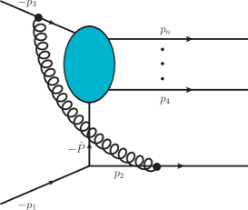
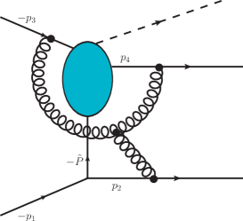
Figure 1: Two-parton factorization breaking correlations at one-loop in hadron–hadron collisions (left). Three-parton factorization breaking correlations at two-loops, $n\geq 4$ QCD partons (right).

3 Squared amplitudes and cross-sections

The all-order singular behaviour of the squared matrix element $|{\cal M}|^{2}$ (summed over the colours and spins of the external partons) in a generic kinematical configuration of $m$ collinear partons is obtained by squaring the generalized factorization formula in Eq. (4):

$$|{\cal M}|^{2}\;\simeq\langle\,{\overline{\cal M}}\,|\,\;{\bf P}(p_{1},\dots,p_{m};{\widetilde{P}};p_{m+1},\dots,p_{n})\;\;|{{\overline{\cal M}}}\rangle\;\;,$$ (16)

where the matrix ${\bf P}$ is the square of the all-order splitting matrix $\mathbf{Sp}$ ,

$${\bf P}\equiv\left[\,{{\mbox{$\mathbf{Sp}$}}}\,\right]^{\dagger}\,{{\mbox{$\mathbf{Sp}$}}}~{},$$ (17)

and it satisfies a loop expansion similar to Eq. (6), with perturbative coefficients ${\bf P}^{(k)}$ $(k=0,1,2,\ldots)$.

The splitting matrix in hadron–hadron collision processes breaks strict collinear factorization beyond the tree-level. However, owing to their absorptive origin, the factorization breaking effects partly cancel for squared amplitudes, and thus a violation of collinear factorization in physical observables is not directly implied. Factorization breaking contributions can cancel either in the squared splitting matrix ${\bf P}$, after taking the expectation value with the reduced matrix element in Eq. (16), or even among different partonic processes with different number of external partons contributing to the same physical cross-section at a given order.

The tree-level collinear matrix ${\bf P}^{(0)}$ is obviously strictly factorized also in the SL region. The divergent part of ${\bf P}^{(1)}$ is strictly factorized because the factorization breaking operator in Eq. (14) is anti-Hermitian. In the two-parton collinear limit also the complete ${\bf P}^{(1)}$, including the IR finite part, is strictly factorized [17], in spite of the fact that ${{\mbox{$\mathbf{Sp}$}}}^{(1)}$ violates collinear factorization. Similarly, the three-parton factorization breaking correlations appearing in the two-parton splitting matrix ${\bf{{\mbox{$\mathbf{Sp}$}}}}^{(2)}$ (Fig. 1 (right)) survive in ${\bf P}^{(2)}$ but only for processes with $n\geq 5$ QCD partons [17].

The expectation value of the two-loop operator ${\widetilde{\Delta}}_{P}^{(2)}(\epsilon)={\widetilde{\Delta}}_{C}^{(2)}(\epsilon)+{\rm h.c.}$, which gives the (IR dominant) factorization breaking contribution to the squared splitting matrix ${\bf P}^{(2)}$ for the two-parton collinear limit , onto the reduced matrix element ${\overline{\cal M}}$ is

$$\!\!\!\!\!\!\!\!\!\!\!\!\!\!\!\langle\,{\overline{\cal M}}\,|\left({{\mbox{$\mathbf{Sp}$}}}^{(0)}\,\right)^{\dagger}\;{\widetilde{\Delta}}_{P}^{(2)}(\epsilon)\;{{\mbox{$\mathbf{Sp}$}}}^{(0)}\;\,|{{\overline{\cal M}}}\rangle=\langle\,{\overline{\cal M}}^{(0)}\,|\left({{\mbox{$\mathbf{Sp}$}}}^{(0)}\,\right)^{\dagger}\;{\widetilde{\Delta}}_{P}^{(2)}(\epsilon)\;{{\mbox{$\mathbf{Sp}$}}}^{(0)}\;|{{\overline{\cal M}}^{(0)}}\rangle$$

$$\;\;+\;\left[\langle\,{\overline{\cal M}}^{(1)}\,|\,\left({{\mbox{$\mathbf{Sp}$}}}^{(0)}\,\right)^{\dagger}\;{\widetilde{\Delta}}_{P}^{(2)}(\epsilon)\;{{\mbox{$\mathbf{Sp}$}}}^{(0)}\;|{{\overline{\cal M}}^{(0)}}\rangle+{\rm c.c.}\;\right]+{\rm higher\;orders}\;\;.$$ (18)

Although ${\widetilde{\Delta}}_{P}^{(2)}$ is not vanishing, its lowest-order expectation value (i.e., the first term on the right-hand side of Eq. (3)) vanishes in pure QCD [18] (i.e., if the lowest-order reduced matrix element ${\overline{\cal M}}^{(0)}$ is produced by tree-level QCD interactions). Note however that this contribution would be non-vanishing, for instance, for tree-level quark–quark scattering produced by electroweak interactions (with CP-violating electroweak couplings and/or finite width of the $Z$ and $W^{\pm}$ bosons), or if the tree-level QCD scattering is supplemented with one-loop (pure) QED radiative corrections.

Therefore, as a matter of principle, it remains true that the operator ${\widetilde{\Delta}}_{P}^{(2)}$ explicitly uncovers two-loop QCD effects that lead to violation of strict collinear factorization at the squared amplitude level. Moreover, the second term in the right-hand side of Eq. (3) is not vanishing and contributes to the SL collinear limit of three-loop QCD squared amplitudes, together with the factorization breaking effect produced by ${\bf P}^{(3)}$ and highlighted independently in Refs. [17, 18]. In the case of scattering amplitudes with $n=5$ QCD partons, the colour correlation structure of these two factorization breaking contributions at three loops is analogous to the commutator structures that were found in the N⁴LO computation of super-leading logarithms in ‘gaps–between–jets’ cross sections [22].

4 Summary

Collinear factorization has been generalized to all orders for kinematical configurations where two or more external partons become collinear, and explicit results on one-loop and two-loop (and three-loop) amplitudes for both the two-parton and multiparton collinear limits have been presented [17]. In the space-like region strict factorization is violated beyond the tree-level for scattering amplitudes. For squared amplitudes the strict-factorization breaking terms partly cancel, but the remaining effects still lead to logarithmically-enhanced contributions at high perturbative orders and challenge the validity of factorization theorems of mass (collinear) singularities.

Acknowlegdements: This work is supported by REA Grant Agreement PITN-GA-2010-264564 (LHCPhenoNet), by UBACYT, CONICET, ANPCyT, INFN, INFN-MICINN agreement AIC-D-2011-0715, MICINN (FPA2007-60323, FPA2011-23778 and CSD2007-00042 CPAN) and GV (PROMETEO/2008/069).

References

- [1] G. Altarelli and G. Parisi, Nucl. Phys. B 126 (1977) 298.
- [2] F. A. Berends and W. T. Giele, Nucl. Phys. B 306 (1988) 759.
- [3] M. L. Mangano and S. J. Parke, Phys. Rept. 200 (1991) 301.
- [4] J. M. Campbell and E. W. N. Glover, Nucl. Phys. B 527 (1998) 264.
- [5] S. Catani and M. Grazzini, Phys. Lett. B 446 (1999) 143; Nucl. Phys. B 570 (2000) 287.
- [6] V. Del Duca, A. Frizzo and F. Maltoni, Nucl. Phys. B 568 (2000) 211.
- [7] T. G. Birthwright, E. W. N. Glover, V. V. Khoze and P. Marquard, JHEP 0505 (2005) 013; JHEP 0507 (2005) 068.
- [8] S. Catani, P. Draggiotis and G. Rodrigo, PoS LL2012 (2012) 054.
- [9] Z. Bern, G. Chalmers, L. J. Dixon and D. A. Kosower, Phys. Rev. Lett. 72 (1994) 2134; Z. Bern, L. J. Dixon, D. C. Dunbar and D. A. Kosower, Nucl. Phys. B 425 (1994) 217.
- [10] Z. Bern and G. Chalmers, Nucl. Phys. B 447 (1995) 465.
- [11] Z. Bern, V. Del Duca and C. R. Schmidt, Phys. Lett. B 445 (1998) 168; Z. Bern, V. Del Duca, W. B. Kilgore and C. R. Schmidt, Phys. Rev. D 60 (1999) 116001.
- [12] D. A. Kosower and P. Uwer, Nucl. Phys. B 563 (1999) 477.
- [13] S. Catani, D. de Florian and G. Rodrigo, Phys. Lett. B 586 (2004) 323.
- [14] Z. Bern, L. J. Dixon and D. A. Kosower, JHEP 0408 (2004) 012.
- [15] S. D. Badger and E. W. N. Glover, JHEP 0407 (2004) 040.
- [16] D. A. Kosower, Nucl. Phys. B 552 (1999) 319.
- [17] S. Catani, D. de Florian and G. Rodrigo, JHEP 1207 (2012) 026.
- [18] J. R. Forshaw, M. H. Seymour and A. Siodmok, arXiv:1206.6363 [hep-ph].
- [19] J. P. Ralston and B. Pire, Phys. Rev. Lett. 49 (1982) 1605; Phys. Lett. B 117 (1982) 233.
- [20] S. Catani, M. Ciafaloni and G. Marchesini, Nucl. Phys. B 264 (1986) 588.
- [21] R. Bonciani, S. Catani, M. L. Mangano and P. Nason, Phys. Lett. B 575 (2003) 268.
- [22] J. R. Forshaw, A. Kyrieleis and M. H. Seymour, JHEP 0608 (2006) 059; JHEP 0809 (2008) 128; J. Keates and M. H. Seymour, JHEP 0904 (2009) 040.
- [23] S. M. Aybat and G. F. Sterman, Phys. Lett. B 671 (2009) 46.
- [24] C. W. Bauer, B. O. Lange and G. Ovanesyan, JHEP 1107 (2011) 077.
- [25] V. Del Duca, C. Duhr, E. Gardi, L. Magnea and C. D. White, JHEP 1112 (2011) 021; Phys. Rev. D 85 (2012) 071104.
- [26] See, J. C. Collins, D. E. Soper and G. F. Sterman, in Perturbative Quantum Chromodynamics, ed. A. H. Mueller, Adv. Ser. Direct. High Energy Phys. 5 (1988) 1, and references therein.
- [27] A. Mitov and G. Sterman, arXiv:1209.5798 [hep-ph].
- [28] C. J. Bomhof, P. J. Mulders and F. Pijlman, Phys. Lett. B 596 (2004) 277; Eur. Phys. J. C 47 (2006) 147; J. Collins and J. W. Qiu, Phys. Rev. D 75 (2007) 114014; J. Collins, arXiv:0708.4410 [hep-ph].
- [29] A. Bacchetta, C. J. Bomhof, P. J. Mulders and F. Pijlman, Phys. Rev. D 72 (2005) 034030; W. Vogelsang and F. Yuan, Phys. Rev. D 76 (2007) 094013.
- [30] T. C. Rogers and P. J. Mulders, Phys. Rev. D 81 (2010) 094006.
- [31] T. Becher and M. Neubert, JHEP 0906 (2009) 081.
- [32] L. J. Dixon, E. Gardi and L. Magnea, JHEP 1002 (2010) 081.
- [33] V. Ahrens, M. Neubert and L. Vernazza, JHEP 1209 (2012) 138.
- [34] S. Catani, Phys. Lett. B 427 (1998) 161.
- [35] G. Sterman and M. E. Tejeda-Yeomans, Phys. Lett. B 552 (2003) 48.
- [36] S. M. Aybat, L. J. Dixon and G. Sterman, Phys. Rev. Lett. 97 (2006) 072001; Phys. Rev. D 74 (2006) 074004.
- [37] L. J. Dixon, L. Magnea and G. Sterman, JHEP 0808 (2008) 022.
- [38] T. Becher and M. Neubert, Phys. Rev. Lett. 102 (2009) 162001.
- [39] E. Gardi and L. Magnea, JHEP 0903 (2009) 079.
- [40] S. Catani and M. H. Seymour, Phys. Lett. B 378 (1996) 287; Nucl. Phys. B 485 (1997) 291 [Erratum-ibid. B 510 (1998) 503].