Correspondence between $f(G)$ Gravity and Holographic Dark Energy via Power-law Solution

Abstract

In this paper, we discuss cosmological application of holographic Dark Energy (HDE) in the framework of $f(G)$ modified gravity. For this purpose, we construct $f(G)$ model with the inclusion of HDE and a well-known power law form of the scale factor $a\left(t\right)$. The reconstructed $f(G)$ is found to satisfy a sufficient condition for a realistic modified gravity model. We find quintessence behavior of effective equation of state (EoS) parameter $\omega_{DE}$ through energy conditions in this context. Also, we observe that the squared speed of sound $v_{s}^{2}$ remains negative which shows the instability of HDE $f(G)$ model.

I Introduction

Accelerated phenomenon of the universe is now well established thanks to many observationsSpergel ; Perlmu . It is suggested in the studies that the universe exhibits spatially flat scenario and contains dark energy (DE) as a major component with negative pressure and 30$\%$ of dust matter consisting of cold dark matter (CDM) plus baryons. The contribution of radiation can be considered practically negligible. For related review works see the references Copeland ; Tsuza . In order to understand the DE nature, it is required to clarify about its candidates either it is a cosmological constant ($\Lambda$) or a form of dynamical model Tsuza . The dynamical DE models can be differentiated from the cosmological constant through the tool of EoS parameter $w_{DE}=p_{DE}/\rho_{DE}$, where the numerator and denominator indicate, respectively, the density and the pressure of DE. Several candidates of DE have been proposed Copeland .

It was shown through the data analysis of SNe Ia that these dynamical models provide more consistency with present scenario of the universe as compare to $\Lambda$. A detailed analysis of DE can be found in 14 . The development in the study of black hole theory and string theory results the holographic principle which states that the number of degrees of freedom of a physical system should be finite, it should scale with its bounding area rather than with its volume and it should be constrained by an infrared cut-off.

The Holographic DE (HDE) is one of the most interesting dynamical model and is based on the holographic principle proposed by 17 . It has also been constrained and tested by various astronomical schemes and with the help of the anthropic principle 27 . By the inclusion of holographic principle into cosmology, it can be found the upper bound of the entropy contained in the universe 17 . Through this bound, Li 28 proposed the constraint on the DE density:

$$\rho_{DE}=3c^{2}M_{p}^{2}L^{-2},$$ (1)

where $c^{2},~{}L,~{}M_{p}=\left(8\pi G\right)^{-1/2}=10^{18}GeV$ indicates a numerical constant, the IR cut-off and the reduced Planck mass, respectively.
There is another form of dynamical DE models which is proposed through large-distance modification of gravity Tsuza . Importance of modified gravity for late acceleration of the universe has been reviewed by Tsuza ; Nojiri1 ; Clifton . In this class, $f(R)$ gravity, $f(T)$ gravity, braneworld models, Galileon gravity, Gauss-Bonnet gravity etc exist. All these theories of modified gravity are thoroughly discussed in Tsuza . The theory of scalar-Gauss-Bonnet gravity, named as $f(G)$ has been proposed by nojiri1 . Since the focus of the present work is $f(G)$ gravity, we explore the existing literature on $f(G)$ gravity. Myrzalulov et al Myrza1 have found that $f(G)$ gravity describes the accelerated expansion phenomenon of the universe and also explain the radiation$/$matter dominated eras. In the same paper, it was shown that $f(G)$ models have ability to reproduce DE and inflation and can be modeled as an inhomogeneous fluid with a dynamical EoS parameter.

In a recent work rastkar , $f(G)$ models from the power law solutions by coupling gravity with perfect fluid has been found. It was observed that a special form of $f(G)$ models exist for a phantom phase of the universe. Garcia et al Garcia considered specific realistic forms of $f(G)$ gravity and presented general inequalities through energy conditions and explored the viability of the various forms of $f(G)$ gravity through cosmographic analysis.

The main purpose of this work is to reconstruct $f(G)$ model by using HDE and check its viability through different cosmological parameters. For this purpose, we assume exact power law solution of scale factor. Also we investigated the validity of energy conditions and stability of the model. We adopt the pattern of the paper as follows. In Section 2, we provide the basic formalism of $f(G)$ gravity and HDE. We reconstruct the HDE $f(G)$ model taking into account the correspondence process. Subsection A inherits the viability of energy conditions for the corresponding model whereas stability of the model is investigated in the subsection B. The results of the paper are summarized in the last Section.

II Correspondence between $f(G)$ gravity and HDE

The $f(G)$ action that describes Einstein’s gravity coupled with perfect fluid plus a Gauss-Bonnet ($G$) term is given by nojiri1 ; rastkar :

$$S=\int d^{4}x\sqrt{-g}\left[\frac{1}{2\kappa^{2}}R+f(G)+\mathcal{L}_{m}\right],$$ (2)

where $G=R^{2}-4R_{\mu\nu}R^{\mu\nu}+R_{\mu\nu\lambda\sigma}R^{\mu\nu\lambda\sigma}$ ($R$ represents the Ricci scalar curvature, $R_{\mu\nu}$ represents the Ricci curvature tensor and $R_{\mu\nu\lambda\sigma}$ represents the Riemann curvature tensor), $\kappa^{2}=8\pi G$, $g$ is the determinant of the metric tensor $g_{\mu\nu}$ and $\mathcal{L}_{m}$ is the Lagrangian of the matter present in the universe. The variation of the action $S$ with respect to $g_{\mu\nu}$ generates the field equations. In this paper, a special form of $f(G)$ gravity proposed by rastkar is being used. In case of flat FRW metric (corresponding to curvature parameter $k=0$), the Ricci scalar curvature $R$ and the Gauss-Bonnet invariant $G$ become, respectively, $R=6(\dot{H}+2H^{2})$ and $G=24H^{2}(\dot{H}+H^{2})$, where the dot represents the time derivative. The first FRW equation (with $8\pi G=1)$ takes the form:

$$H^{2}=\frac{1}{3}(Gf_{G}-f(G)-24\dot{G}H^{3}f_{GG}+\rho_{m})=\frac{1}{3}(\rho_{G}+\rho_{m}),$$ (3)

where $f_{G}=\frac{df}{dG}$ and $f_{GG}=\frac{d^{2}f}{dG^{2}}$. Earlier, Setare Setare1 reconstructed $f(R)$ gravity from HDE. In this Section, we shall discuss a reconstruction of the above form of $f(G)$ gravity in HDE framewok. The HDE density is defined as: Setare1

$$\rho_{\Lambda}=\frac{3c^{2}}{R_{h}^{2}},$$ (4)

where $R_{h}$ represents the future event horizon which is defined as:

$$R_{h}=a\int_{t}^{\infty}\frac{dt}{a}=a\int_{a}^{\infty}\frac{da}{Ha^{2}}.$$ (5)

The dimensionless DE density is defined by the critical energy density $\rho_{cr}=3H^{2}$ as follow:

$$\Omega_{\Lambda}=\frac{\rho_{\Lambda}}{\rho_{cr}}=\frac{c^{2}}{R_{h}^{2}H^{2}}.$$ (6)

The derivative of $R_{h}$ with respect to the cosmic time $t$ is given by:

$$\dot{R}_{h}=R_{h}H-1=\frac{c}{\sqrt{\Omega_{\Lambda}}}-1.$$ (7)

Using the conservation equation, the EoS parameter for HDE is obtained by Setare1 as follow:

$$\omega_{\Lambda}=-\left(\frac{1}{3}+\frac{2\sqrt{\Omega_{\Lambda}}}{3c}\right).$$ (8)

If the universe is dominated by the HDE, i.e., $\Omega_{\Lambda}\rightarrow 1$, then we observe different conditions on $c$. The $\omega_{\Lambda}$ represents the quintessence like behavior for $c>1$ while phantom dominated universe $(\omega_{\Lambda}<-1)$ is observed for the values of $c$ less than $1$. For $c=1$, the EoS parameter of HDE indicates the de Sitter phase of the universe. Hence the value of $c$ is important in the evolving universe dominated by HDE. In order to apply the correspondence, we equate $\rho_{G}=\rho_{\Lambda}$. It follows that:

$$3H^{2}\Omega_{\Lambda}=Gf_{G}-f(G)-24\dot{G}H^{3}f_{GG},$$ (9)

yielding:

$$f(G)=Gf_{G}-3H^{2}\Omega_{\Lambda}-24\dot{G}H^{3}f_{GG}.$$ (10)

Here we assume the scale factor $a\left(t\right)$ in the form of exact power law solution of the field equation as Setare1 :

$$a(t)=a_{0}(t_{s}-t)^{\gamma},$$ (11)

where, $a_{0}$, $t_{s}$ and $\gamma$ are constants. In particular, $a_{0}$ represents the present day value of the scale factor and $t_{s}>t$ is the future singularity finite time. This type of scale factor may give the sudden singularity (type II) or singular curvature and $\dot{H}$ (type IV) for positive $\gamma$. With this choice of scale factor, the Hubble parameter $H$ and $G$ become, respectively, $H=-\frac{\gamma}{t_{s}-t}$ and $G=\frac{24(\gamma-1)\gamma^{3}}{(t_{s}-t)^{4}}$. Inserting Eq. (11) in Eq. (10), we can rewrite the differential equation given in Eq. (10) as follow:

$$\frac{2304(\gamma-1)\gamma^{6}}{(t_{s}-t)^{8}}f_{GG}+\frac{24\gamma^{3}(\gamma-1)}{(t_{s}-t)^{4}}f_{G}-f(G)=\frac{3\gamma^{2}-3c^{2}(\gamma-1)^{2}}{(t_{s}-t)^{2}}.$$ (12)

In terms of $G$, Eq. (12) can be rewritten as:

$$\frac{4}{\gamma-1}G^{\frac{3}{2}}f_{GG}+\sqrt{G}f_{G}-G^{-\frac{1}{2}}f(G)=\frac{3\gamma^{2}-3c^{2}(\gamma-1)^{2}}{\sqrt{24\gamma^{3}(\gamma-1)}},$$ (13)

which is a differential equation of order two which solution is given by:

$$f(G)=-\frac{8}{\gamma+1}\sqrt{G}+G\left(G^{-\frac{3+\gamma}{4}}C_{1}+C_{2}\right),$$ (14)

where $C_{1}$ and $C_{2}$ are integration constants. This is the $f(G)$ model in the HDE scenario with power-law form of scale factor.

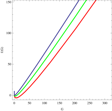
Figure 1: Evolution of HDE $f(G)$ model versus $G$ with power-law scale factor. Red, Green and Blue lines correspond, respectively, to $\gamma=1.02,~{}2.2~{}\textrm{and}~{}5.2$.

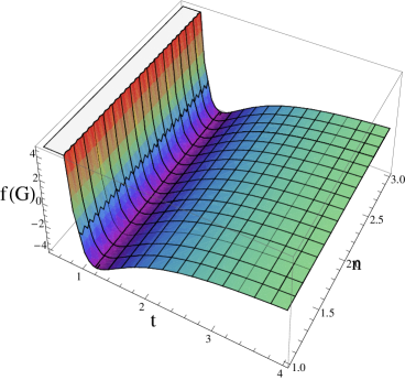
Figure 2: Evolution of HDE $f(G)$ model versus $t$ for a range of values of $\gamma$.

We plot $f(G)$ model against $G$ as shown in Figure 1. We find that $f(G)$ is exhibiting increasing pattern with increasing $G$. Furthermore, we observe that

$$\lim_{G\rightarrow 0}f(G)=0.$$ (15)

This is a sufficient condition to ensure that HDE $f(G)$ model is a realistic model rastkar . Hence, the reconstructed $f(G)$ given in Eq. (14) is a consistent modified gravity with HDE in flat space. The $f(G)$ model can be interpreted as a function of cosmic time in the following way:

$$f(G) = -\frac{16\sqrt{6}}{\gamma+1}\sqrt{\frac{(\gamma-1)\gamma^{3}}{(t_{s}-t)^{4}}}$$ (16)

$$+ \frac{24\gamma^{3}(\gamma-1)}{(t_{s}-t)^{4}}\left[C_{2}+C_{1}2^{-\frac{3(3+\gamma)}{4}}3^{-\frac{\gamma+3}{4}}\left(\frac{(\gamma-1)\gamma^{3}}{(t_{s}-t)^{4}}\right)^{-\frac{3+\gamma}{4}}\right].$$

Figure 2 represents the graph of HDE $f(G)$ model versus $t$ for a range of values of $\gamma>1$. Initially, it shows a decreasing behavior and it assumes negative values. After a short interval, we find the increment in $f(G)$ and it becomes positive. Hence, the model given in Eq. (16) describes the decaying process firstly and then starts increasing, becomes positive during the evolution of the universe.

In the subsequent Section we shall consider the energy conditions and stability of the reconstructed HDE $f(G)$ gravity model.

II.1 Energy conditions for HDE $f(G)$ gravity

We now find the energy conditions for reconstructed $f(G)$ gravity in HDE scenario. In context of modified theories of gravity, the phenomenon of energy conditions have been widely studied C . Its various forms, namely null energy condition (NEC), weak energy condition (WEC), dominant energy condition (DEC) and strong energy condition (SEC) are found through attractiveness of gravity along with Raychaudhuri equation Garcia ; C . The expansion sceanrio of the universe E , phantom field potential F and evolution of the deceleration parameter $q$ G have been explored using these conditions in general relativity. Sadeghi et al. H and Garcia et al. Garcia investigated the viability of some specific forms of $f(G)$ model by using approximated current values of Hubble, jerk, deceleration and snap parameters with the help of these conditions. They also explored that the late-time de-Sitter solution is stable and the investigated the existence of standard radiation/matter dominated eras through WEC and SEC. Using effective approach, the energy conditions are given, respectively, by Garcia :

• NEC: $\rho_{eff}+p_{eff}\geq 0$,

• WEC: $\rho_{eff}\geq 0,\quad\rho_{eff}+p_{eff}\geq 0$,

• DEC: $\rho_{eff}\geq 0,\quad\rho_{eff}\pm p_{eff}\geq 0$,

• SEC: $\rho_{eff}+3p_{eff}\geq 0,\quad\rho_{eff}+p_{eff}\geq 0$.

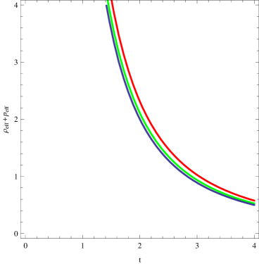
Figure 3: Behaviour of $\rho_{eff}+p_{eff}$ versus $t$ for different values of $\gamma>1$.

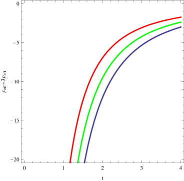
Figure 4: Behaviour of $\rho_{eff}+3p_{eff}$ versus $t$ for different values of $\gamma>1$.

The NEC and the WEC are simple and important in the sense that the violation of NEC results to the violation of remaining energy conditions. It guarantees the validity of second law of thermodynamics and it represents the reduction of energy density with expansion of the universe. However, the violation of SEC represents the accelerated expansion of the universe. For HDE $f(G)$ gravity, the effective energy density and the effective pressure are obtained as

$$\rho_{eff} = \rho_{m}+\frac{1}{2}\left\{G(C_{2}+C_{1}G^{-\frac{3+\gamma}{4}})+6H^{2}+24H^{3}f(G)\dot{G}-\frac{8\sqrt{G}}{1+\gamma}\right.$$ (17)

$$- \left.G^{2}\left[G(C_{2}+C_{1}G^{-\frac{3+\gamma}{4}})-\frac{8\sqrt{G}}{\gamma+1}\right]\right\},$$

$$p_{eff} = p_{m}+\frac{1}{2}\left\{G(C_{2}+C_{1}G^{-\frac{3+\gamma}{4}})-\frac{8\sqrt{G}}{\gamma+1}+4608H^{4}(H\ddot{H}+4H^{2}\dot{H}+2\dot{H}^{2})^{2}\right.$$ (18)

$$\times \left.\left[\frac{1}{16}C_{1}G^{-\frac{11+\gamma}{4}}(\gamma+3)(\gamma+7)-\frac{1}{64}C_{1}G^{-\frac{11+\gamma}{4}}(\gamma+7)(\gamma+3)^{2}-\frac{3}{G^{\frac{5}{2}}(1+\gamma)}\right]\right.$$

$$+ \left.192H^{2}(H^{2}\dddot{H}+6H^{3}\ddot{H}+8H^{4}\dot{H}+8\dot{H}\ddot{H}+24H^{2}\dot{H}^{2}+6\dot{H}^{3})\left[\frac{C_{1}(3+\gamma)(\gamma-1)G^{-\frac{7+\gamma}{16}}}{4}\right.\right.$$

$$+ \left.\left.\frac{2}{G^{\frac{3}{2}}(\gamma+1)}\right]-24H^{2}(\dot{H}+H^{2})\left[C_{2}-\frac{\gamma-1}{4}C_{2}G^{-\frac{3+\gamma}{4}}-\frac{4}{\sqrt{G}(\gamma+1)}\right]\right\}.$$

The plot of NEC for HDE $f(G)$ model versus cosmic time $t$ taking different values of $\gamma$ is shown in Figure 3. We see that for all values of $\gamma$, $\rho_{eff}+p_{eff}>0\Rightarrow~{}w_{eff}>-1$. This indicates the validity of NEC as well as WEC. Figure 4 represents the plot of SEC versus $t$ for HDE $f(G)$ model for the same values of $\gamma$. Initially, $\rho_{eff}+3p_{eff}$ describes the increasing but negative behavior. With the passage of time, the model shows the flatness in the curves for all values of $\gamma$ and inherits negative behavior of $\rho_{eff}+3p_{eff}$. It gives the violation of SEC as $\rho_{eff}+3p_{eff}<0\Rightarrow w_{eff}<-\frac{1}{3}$ and it ensures the accelerated expansion of the universe. Thus, combining both conditions on the effective EoS parameter, we have $-1<w_{eff}<-\frac{1}{3}$. This indicates quintessence-like behavior of the EoS parameter for HDE $f(G)$ model.

II.2 Stability of reconstructed $f(G)$ gravity

We now consider an important quantity to check the stability of HDE $f(G)$ model, namely the squared speed of sound $v_{s}^{2}$, defined as:

$$v_{s}^{2}=\frac{\dot{p}_{\Lambda}}{\dot{\rho}_{\Lambda}}$$ (19)

The sign of $v_{s}^{2}$ is crucial for stability of a background evolution. A negative value implies a classical instability of a given perturbation in general relativity myung ; kim . Myung myung has observed that $v_{s}^{2}$ for HDE is always negative for the future event horizon as IR cutoff, while for Chaplygin gas and tachyon, it is observed non-negative. Kim et al. kim found that the squared speed of sound for agegraphic DE is always negative leading to the instability of the perfect fluid for the model. Also, it was found that the ghost QCD 20g DE model is unstable. Recently, Sharif and Jawad sharif have shown that interacting new HDE is characterized by negative $v_{s}^{2}$.

We plot $v_{s}^{2}$ versus $t$ taking the power-law scale factor in the HDE $f(G)$ model as shown in Figure 5. Here, we consider $v_{s}^{2}$ as a ratio of the effective pressure and energy densities given, respectively, in Eqs. (17) and (18), i.e. $v_{s}^{2}=\frac{\dot{p}_{eff}}{\dot{\rho}_{eff}}$. We observe that it remains negative for the present and future epoch. This shows that $f(G)$ model in HDE scenario with power-law scale factor is classically unstable.

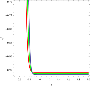
Figure 5: Behaviour of $v_{s}^{2}$ for different values of $\gamma>1$.

III Conclusions

Many different candidates have been proposed as possible candidates of DE. Modified gravity has recently emerged as a possible unification of DE and DM. This work aims at a cosmological application of HDE density in the framework of a modified gravity, named as $f(G)$ gravity. In this framework, we have considered the EoS parameter $\omega_{DE}$ of the HDE density. We have developed a correspondence between the energy densities of $f(G)$ gravity and HDE and obtained a second order differential equation which was solved for $f(G)$ with the help of power-law form of scale factor $a$. The validity of NEC and SEC is investigated for this model and stability is checked through squared speed of sound $v_{s}^{2}$.

We have found that the obtained model given in Eq. (14) is a consistent modified gravity model with HDE in flat space. It gives an increasing behavior with the passage of time. The NEC as well as the WEC are always hold while SEC is violated for this model. The violation of SEC gives $-1<w_{eff}<-\frac{1}{3}$ which shows the quintessence epoch of the accelerated expansion of the universe. Also the reconstructed HDE $f(G)$ model always remain instable like HDE with event horizon as IR cutoff and interacting new HDE models.

III.1 Acknowledgements

One of the authors (SC) sincerely acknowledges the facilities provided to him by the Inter-University Centre for Astronomy and Astrophysics (IUCAA), Pune, India, during his visit in November, 2012 under the Visitor Associateship Programme. Financial support from DST, Govt. of India under project SR/FTP/PS-167/2011 is duely acknowledged by SC.

References

- (1) D. N. Spergel et al., Astrophys. J. Suppl. 148 175 (2003).
- (2) S. Perlmutter et al., Astrophys. J. 517 565 (1999).
- (3) E. J. Copeland, M. Sami and S. Tsujikawa, Int. J. Mod. Phys. D 15 1753 (2006).
- (4) S. Tsujikawa, Lect. Notes Phys. 800 99 (2010).
- (5) M. Li et al., Commun. Theoret. Phys. 56 525 (2011).
- (6) W. Fischler and L. Susskind, arXiv:hep-th/9806039.
- (7) Q. -G. Huang and M. Li, JCAP 3 1 (2005)
- (8) M. Li, Phys. Lett. B 603 1 (2004).
- (9) S. Nojiri, and S. D. Odintsov, Int. J. Geom. Meth. Mod. Phys. 4 115 (2007).
- (10) T. Clifton, P. G. Ferreira, A. Padilla and C. Skordis, Physics Reports 513 1 (2012).
- (11) S. Nojiri and S. D. Odintsov, Phys. Lett. B 631 1 (2005).
- (12) R. Myrzakulov, D. S ez-G mez and A. Tureanu, Gen. Relativ. Gravit. 43 1671 (2011).
- (13) A. R. Rastkar, M. R. Setare and F. Darabi, Astrophys. Space Sci. 337 487 (2012).
- (14) N. M. Garcia, T. Harko, F. S. N. Lobo and J. P. Mimoso, Phys. Rev. D 83 104032 (2011).
- (15) M. R. Setare, Int. J. Mod. Phys. D 12 2219 (2008).
- (16) J. Santos et al., Phys. Rev. D 76 083513 (2007); D. Liu and M. J. Reboucas, Phys. Rev. D (2012, to appear); F. G. Alvarenga et al., J. Mod. Phys. (2012, to appear) arXiv:1205.4678; M. Sharif, S. Rani and R. Myrzakulov, arXiv: 1210.2714.
- (17) A. A. Sen and R. J. Scherrer, Phys. Lett. B 659 457 (2008); J. Santos et al., Phys. Rev. D 76 043519 (2007).
- (18) J. Santos and J. S. Alcaniz, Phys. Lett. B 619 11 (2005).
- (19) Y. Gong and A. Wang, arXiv:0705.0996v1.
- (20) J. Sadeghi, A. Banijamali and H. Vaez, Int. J. Theor. Phys. 51 2888 (2012).
- (21) K. Y. Kim, H. W. Lee and Y. S. Myung, Phys. Lett. B 660 118 (2008).
- (22) Y. S. Myung, Phys. Lett. B, 652 223 (2007).
- (23) E. Ebrahimi and A. Sheykhi, Int. J. Mod. Phys. D 20 2369 (2011).
- (24) M. Sharif and A. Jawad, Eur. Phys. C 72 2097 (2012).