Coalescence of Liquid Drops: Different Models Versus Experiment

Abstract

The process of coalescence of two identical liquid drops is simulated numerically in the framework of two essentially different mathematical models, and the results are compared with experimental data on the very early stages of the coalescence process reported recently. The first model tested is the ‘conventional’ one, where it is assumed that coalescence as the formation of a single body of fluid occurs by an instant appearance of a liquid bridge smoothly connecting the two drops, and the subsequent process is the evolution of this single body of fluid driven by capillary forces. The second model under investigation considers coalescence as a process where a section of the free surface becomes trapped between the bulk phases as the drops are pressed against each other, and it is the gradual disappearance of this ‘internal interface’ that leads to the formation of a single body of fluid and the conventional model taking over. Using the full numerical solution of the problem in the framework of each of the two models, we show that the recently reported electrical measurements probing the very early stages of the process are better described by the interface formation/disappearance model. New theory-guided experiments are suggested that would help to further elucidate the details of the coalescence phenomenon. As a by-product of our research, the range of validity of different ‘scaling laws’ advanced as approximate solutions to the problem formulated using the conventional model is established.

I Introduction

The phenomenon of coalescence where two liquid volumes, in most cases drops, merge to form a single body of fluid exhibits a range of surprisingly complex behaviour that is important to understand from both the theoretical viewpoint as well as with regard to a large number of applications. The dynamics of coalescing drops is central for a whole host of processes such as viscous sintering(bellehumeur04, ), emulsion stability(dreher99, ), spray cooling(grissom81, ), cloud formation(kovetz69, ), and, in particular, a number of emerging micro- and nanofluidic technologies(quake05, ). The latter include, for example, the 3D-printing devices developed for the rapid fabrication of custom-made products ranging from hearing aids through to electronic circuitry (derby10, ; singh10, ). In this technology, structures are built by microdrops ejected from a printer; these drops subsequently come into contact with a surface containing both dry solid substrate as well as liquid drops deposited earlier, so that being able to predict the behaviour of drops as they undergo stages of both spreading over a solid and coalescence is critical to improving the overall quality of the finished product.

The spatio-temporal scales characterizing the coalescence process are extremely small, so that resolving the key (initial) stages of the process experimentally is very difficult. This is particularly the case in microfluidics where the process of coalescence as such is inseparable from the overall dynamics. This difficulty, and the associated cost of performing high-accuracy experiments, becomes a strong motivation for developing a reliable theoretical description of this class of flows which would be capable of taking one down to the scales inaccessible for experiments and allow one, in particular, to map the parameter space of interest to determine, say, critical points at which the flow regime bifurcates.

From a fundamental perspective, the phenomenon of coalescence is a particular case from a class of flows where the flow domain undergoes a topological transition in a finite time, so that studying this phenomenon might help to elucidate common features and develop methods of quantitative modelling applicable to other flows in this class. Technically, coalescence is the process by which two liquid volumes that at some initial moment touch at a point or along a line, i.e. have a common boundary point or points, become one body of fluid, where (a) there are only ‘internal’ (bulk) and ‘boundary’ points and (b) every two internal points can be connected by a curve passing only through internal points. Once the coalescence as defined above has taken place, the subsequent process is simply the evolution of a single body of liquid and it can be described in the standard way.

In the conventional framework of fluid mechanics, the free surface has to be smooth as otherwise, to compensate the action of the surface tension on the singularities of the free-surface curvature, one has to admit non-integrable singularities in the bulk-flow parameters (richardson68, ). Therefore, when applied to the coalescence phenomenon, the conventional approach essentially by-passes the problem: it is assumed that immediately after the two free surfaces touch, there somehow appears a smooth liquid bridge of a small but finite size connecting the two fluid volumes (Figure 1). In other words, the coalescence, i.e. the formation of a single body of fluid, has already taken place and the subsequent evolution of the free-surface shape can be treated conventionally. Hence, theoretical studies of coalescence in the framework of conventional fluid mechanics essentially boil down to a ‘backward analysis’ of the process, i.e. to considering what happens in the limit $t\to 0+$ as the time is rolled back to the initial singularity in order to uncover what the early stages of the evolution of the free surface and the flow parameters might be.

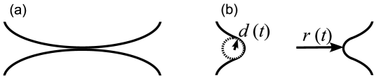
Figure 1: Sketch illustrating the scheme used in the conventional modelling of coalescence: the initial contact (a) is instantly followed by a finite-size ‘bridge’ connecting the two fluid volumes (b), i.e. $r(0)=r_{min}>0$. The subsequent evolution of the single body of fluid is driven by the capillary pressure, where the main contribution is due to the longitudinal curvature $1/d(t)$.

In the forthcoming subsections, we will describe how the development of new experimental techniques and a new generation of experimental equipment, in particular the use ultra high-speed optical cameras (thoroddsen05, ) as well as novel electrical methods (paulsen11, ), have made it possible to study processes on the spatio-temporal scales that were previously unobtainable. Therefore, this is a perfect opportunity for a detailed comparison between theory and experiment in order to probe the fundamental physics associated with this ‘singular’ free-surface flow.

II Background

II.1 Plane 2D flows

Much initial work on coalescence was motivated by Frenkel’s 1945 paper on viscous sintering (frenkel45, ) for inertialess viscous flow with an inviscid dynamically passive gas in the exterior. Later, consideration of the plane 2-dimensional flow of high viscosity liquids led, in particular, in the works of Hopper(hopper84, ; hopper90, ; hopper93a, ; hopper93b, ) and Richardson(richardson92, ), to an exact solution for coalescing cylinders obtained using conformal mapping techniques. Notably, as pointed out in (eggers99, ), in this solution, for small radii of the liquid bridge one has that the radius of longitudinal curvature $d(t)=O(r^{3})$ as $r\to 0+$ (Figure 1), i.e. it is asymptotically even smaller than the undisturbed distance between the free surfaces, which is of $O(r^{2})$ as $r\to 0+$. In other words, exact solutions obtained in the framework of conventional fluid mechanics confirmed that this formulation predicts that the free-surface curvature is singular as $t\to 0+$ and hence the conventional model is used beyond its limits of applicability through the initial stage of the process. Correspondingly, the flow velocity in the exact solution is also singular as $t\to 0+$ and unphysically high for small $t$ and $r$.

II.2 Scaling laws for axisymmetric flows

More recent works have been mainly concerned with deriving various ‘scaling laws’ for the radius of the liquid bridge $r(t)$, joining two drops of initial radius $R$, as a function of time $t$ (Figure 1). These scaling laws are obtained by balancing the factors driving and resisting the fluid motion, with the appropriate assumptions about how these factors can be expressed quantitatively.

From a theoretical viewpoint, consideration of scaling laws is analogous to the approach of Frenkel, as opposed to the rigorous fluid mechanical treatment of coalescence initiated by Hopper and Richardson, since, as in Frenkel’s paper(frenkel45, ), to obtain the scaling laws, the solution of the equations of fluid mechanics is found using some plausible assumptions rather than being obtained directly. On the other hand, however, the simple results obtained using the scaling laws approach, once tested experimentally, can give an indication as to whether the rigorous analysis of a given problem formulation is worth pursuing.

Analytic progress has been achieved by assuming that the process is driven by surface tension $\sigma$ and opposed either by viscous or inertial forces (eggers99, ). The driving force due to the surface tension is calculated by assuming that the mean curvature $\kappa$ of the free surface is due primarily to the longitudinal curvature $1/d(t)$ (Figure 1): $\kappa\propto 1/d(t)$. In the inertia-dominated case, it is assumed in (eggers99, ) that $d(t)$ is determined by the initial free surface shape, which for coalescing spheres gives $d\propto r^{2}/R$. As mentioned above, in the viscosity-dominated regime it is shown in (eggers99, ) that when the surrounding gas is inviscid, one has $d(t)\propto r^{3}/R$. In either case, one can calculate the surface tension force $\sigma\kappa(t)$ as a function of time. In the situation where viscous forces dominate inertial ones and hence are the main factor resisting the flow, a scale for velocity is $U_{visc}=\sigma/\mu$ (so that the capillary number $Ca=\mu U_{visc}/\sigma=1$) and the corresponding time scale is $T_{visc}=R\mu/\sigma$. Alternatively, if it is the inertial forces that are the main factor resisting the motion, a scale for velocity is $U_{inert}=(\sigma/\rho R)^{1/2}$ (so that the Weber number $We=\rho U_{inert}^{2}R/\sigma=1$) and the corresponding time scale is $T_{inert}=(\rho R^{3}/\sigma)^{1/2}$. In the viscous case, the simplest scaling is that the bridge radius evolves as $r/R\propto t/T_{visc}$; however, in (eggers99, ) it is shown that there is a logarithmic correction to this term so that

$$r/R=-C_{visc}\left(t/T_{visc}\right)\ln\left(t/T_{visc}\right),$$ (1)

where $C_{visc}$ is a constant. The limits of applicability of this scaling, based on the equivalence of the two- and three-dimensional problems, is expected to hold(eggers99, ) for $r/R<0.03$.

In (eggers99, ), it is suggested that when the Reynolds number, based on $U_{visc}$ as the scale for velocity and the radius of the bridge $r$ as the length scale, becomes of order one, $Re_{r}=\rho\sigma r/\mu^{2}\approx 1$, there will be a crossover point where the dynamics switches from Stokesian to Eulerian, i.e. the main factor resisting the motion is now inertia of the fluid. This crossover point correspond to $r\approx\mu^{2}/(\rho\sigma)$ after which the balance of the surface tension and inertia forces gives

$$r/R=C_{inert}\left(t/T_{inert}\right)^{1/2},$$ (2)

where $C_{inert}$ is a constant. Notably, for water the crossover from viscous to inertial scaling is predicted to occur at $r=14$ nm.

II.3 Numerical simulations

The use of computational simulation for what is, strictly speaking, the evolution of the post-coalescence single body of fluid has focussed both on the very early stages of the process as well as on the global dynamics of the two drops (duchemin03, ; eggers99, ; menchacarocha01, ; paulsen12, ). In the early stages, computations of the inviscid flow, using boundary integral methods, have shown the formation of toroidal bubbles trapped inside the drops as the two free surfaces reconnect themselves in front of the bridge (oguz89, ; duchemin03, ). The appearance of these bubbles, originally suggested in (oguz89, ), has been further investigated in (duchemin03, ) using inviscid boundary integral calculations, and an attempt has been made to continue the simulation past the toroidal bubble formation. It was shown that, despite the bubble generation, the scaling (2) still holds, with the prefactor determined to be $C_{inert}=1.62$ for the period in which bubble formation occurs ($r/R<0.035$). However, as the authors acknowledge, the computational approach for dealing with the reconnection procedure is not entirely satisfactory, with the robust simulation of such phenomena remaining an open problem.

Simulations of the entire post-coalescence process have been performed to varying degrees of accuracy, dependent in many cases on the computational power available at the time, in (jagota88, ; martinez95, ; menchacarocha01, ). A recurring question in these studies was how to initialize the simulation. For example, in (menchacarocha01, ), it is assumed that the singular curvature at the moment of touching of the two fluid volumes is immediately smoothed out over a grid-size dependent region, so that as the grid is refined, the radius of curvature decreases, i.e. the curvature tends to the required singular initial condition. This behaviour is reflected in Figure 9 of (menchacarocha01, ), showing the bridge radius versus time, where changing the grid resolution changes the results considerably, i.e., as expected, the solution is mesh-dependent. A similar approach is used in (paulsen12, ); however, there, the results from the simulation are only plotted when the “transients from the initial conditions have decayed” (see Figure 3 of this paper), so that it is difficult to observe the influence of the initial conditions. Due to an inability to resolve multiscale phenomena computationally, until now, no studies have considered in detail both the very initial stages of coalescence alongside the global dynamics of the drops.

II.4 Experimental data

Several experimental studies have probed the dynamics of coalescing drops. The study of coalescing free liquid drops (Figure 2a) is rather complicated, as it is difficult to control and monitor the movement of the drops with the required precision. Therefore, since coalescence as such is a local process, a common experimental setup is based on using supported hemispherical drops, with one drop sitting on a substrate, or being grown from a capillary tube, and the other, a pendent drop, being grown from a capillary above (Figure 2b). As coalescence is initiated, the bridge radius is then measured as a function of time either optically or using some indirect methods. To date the most exhaustive study of coalescence, using the aforementioned experimental setup, has been carried out by Thoroddsen and co-workers(thoroddsen05, ), who investigated a range of viscosities and drop sizes, with the shapes of the drop monitored using ultra high-speed cameras capable of capturing up to one million frames per second. Similar experiments have been reported in (aarts05, ) and (wu04, ) with the same setup.

As shown in (thoroddsen05, ), after correcting the initial shapes of the drops to account for the influence of gravity, the inviscid scaling law (2) appears to be in good agreement with experimental results for the initial stages of the coalescence of drops of low viscosity ($\mu<10$ mPa s) fluid. It is found in (aarts05, ; wu04, ) that the prefactor $C_{inert}=1.62$ predicted in (duchemin03, ) is considerably higher than all the values obtained experimentally, which for hemispherical drops are seen to be around $C_{inert}=0.8$. Also, no toroidal bubbles have been observed. At intermediate viscosities ($40$ mPa s$~{}<\mu<220$ mPa s), it is found in (thoroddsen05, ) that neither the inertial nor viscous scalings are able to fit the data whilst at the highest viscosity ($\mu=493$ mPa s) a region of linear growth of the bridge radius with time is observed. In both (thoroddsen05, ) and (aarts05, ), linear growth in the initial stages shows no signs of the logarithmic correction as in equation (1). Instead, the scaling $r/R=Bt/T_{visc}$ is shown to fit the data best, where $B$ is the coefficient of proportionality. Notably, the value of the constant $B$ is seen to be a factor of two smaller in (aarts05, ) than in (thoroddsen05, ).

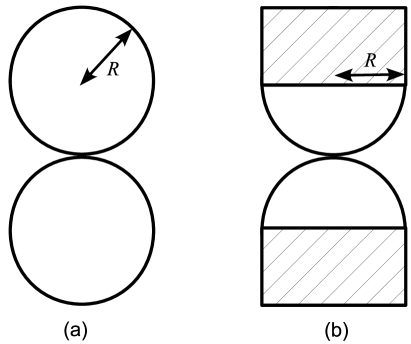
Figure 2: (a): Sketch of the benchmark problem of the coalescence of two free identical liquid spheres. (b): typical experimental setup where drops are grown from capillaries until they begin to coalesce.

Recently, a new experimental technique has been developed to study the coalescence phenomenon at spatio-temporal scales inaccessible to optical measurements. In (case08, ; case09, ; paulsen11, ), an electrical method, extending the techniques utilized in (burton04, ) to study drop pinch-off dynamics, has been used to measure the radius of the bridge connecting two coalescing drops of an electrically conducting liquid down to time scales of $\sim 10$ ns, giving at least two orders of magnitude better resolution than optical techniques. In doing so, it is shown that the initial radius of contact is very small, as suggested in (aarts05, ), so that there is no evidence for the initial area of $\sim 100$ $\mu$m suggested in (thoroddsen05, ). It is noted that the method loses accuracy towards the end of the process ($t>400$ $\mu$s for water), but that in this range optical experiments are available and reliable, so that by using both electrical measurements alongside optical ones, it is possible to obtain accurate measurements over the entire range of bridge radii (see Figure 11 below where we do precisely this).

In (case08, ; case09, ), it is found that for low viscosity fluids a new regime exists for $t<10$ $\mu$s which is inconsistent with the assumption that the inertial scaling, equation (2), will kick-in almost instantaneously for such liquids. In (paulsen11, ), the same electrical method is used to measure the influence of viscosity on the coalescence dynamics, with other parameters (surface tension, density, drop size) almost constant, and similar behaviour is observed over two orders of magnitude variation in the viscosity of water-glycerol mixtures, with, as before, the cross-over time between different flow regimes being vastly different from what the combination of scaling laws predicts. It is suggested in (paulsen11, ) that this is because the cross-over from regimes is based on the Reynolds number whose length scale is taken to be the bridge radius, whereas, in fact it should be based on the undisturbed free surface height at a given radius, which is proportional to $r^{2}$ as opposed to $r$, giving a much later cross-over time, as observed experimentally.

Thus, although in experiments one can observe some of the general trends following from the scalings (1) and (2), experimental studies have been unable to validate these scaling laws. At low viscosities, the prefactor obtained in (duchemin03, ) for small bridge radii has not been confirmed; at intermediate viscosities, neither inertial nor viscous forces can be neglected so that both scaling laws become inapplicable; whilst at the highest viscosities, logarithmic corrections have not been observed and different experiments give different values of the prefactor to a linear power law, which has not been predicted by theory. It should also be pointed out that when using power laws, there is no guarantee that the prefactor which fits the experimental data is necessarily the one that would be obtained from solving the full problem formulation. Thus, it is clear that full-scale computational simulation of this class of flows is called for. Such a simulation will allow one to accurately compare theoretical predictions with experimental data and hence, first of all, show whether or not the model itself accounts for all the key physics involved in the coalescence process. As a by-product, the simulation will be able to test the validity of the scalings (1) and (2) by comparing them to the exact solution.

II.5 Coalescence as an interface formation/disappearance process

In order to study coalescence over a range of viscosities for a sustained period of time and to test the mathematical model of the phenomenon, as opposed to different approximations, against experiments we need to use computational methods that are capable of solving the full Navier-Stokes equations with the required accuracy. This would allow one not only to account in full for the effects of inertia, capillarity and viscosity and hence make the comparison of the conventional model with experiments conclusive; it will also make it possible to incorporate and test against experiments the ‘extra’ physics that carries the system through the topological transition, which is, technically, what coalescence actually is and what is not considered in the conventional model.

As pointed out in the Introduction, the conventional fluid mechanics model essentially deals with the post-coalescence process, i.e. the evolution of a single body of fluid that the coalescence phenomenon has produced, and, as the limit $t\to 0+$ is taken, gives rise to unphysical singularities. This suggests that some ‘additional’ physics, not accounted for in the conventional model, takes the system through the topological change, and the conventional physics takes over when the liquid bridge between the two drops already has a finite size determined by this ‘additional’ physics. The first study identifying this ‘additional’ physics, which was aimed at embedding coalescence into the general physical framework as a particular case of a more general physical phenomenon, has been reported in (shik00, ). It has been shown that coalescence is in fact a particular case of the interface formation/disappearance process: as the two drops are pressed against each other, a section of their free surfaces becomes trapped between the bulk phases (Figure 3). As this trapped interface gradually (albeit, in physical terms, very quickly) loses its surface properties (such as the surface tension), the angle $\theta_{d}$ (Figure 3) formed by each of the free surfaces of the drops with the ‘internal interface’ sandwiched between the two drops goes to $90^{\circ}$, so that eventually a bridge of a finite physically-determined radius emerges and the conventional model takes over. The outlined physics allows for the existence of a non-smooth free surface without unphysical singularities in the flow field since the surface tensions acting on the line where the free-surface curvature is singular are balanced not by the bulk stress, as in (richardson68, ), but by the (residual) surface tension in the ‘internal’ interface. The existence of such non-smooth free surfaces has been confirmed experimentally (joseph91, ) and has already been described theoretically using the above approach (shik00, ; shik05a, ).

The approach outlined above removes the unphysical singularities in the mathematical description of the coalescence process and allows one to treat it in a regular way, as just one of many fluid mechanics phenomena. The developed model (which came to be known as ‘interface formation model’ or, for brevity, IFM) unifies the mathematical modelling of such seemingly different phenomena as coalescence (shik00, ), breakup of liquid threads (shik00, ; shik05b, ) and free films (shik05c, ), as well as dynamic wetting (shik93, ; shik97, ; shik06, ; shik97a, ); an exposition of the fundamentals of the theory of capillary flows with forming/disappearing interfaces can be found in (shik07, ).

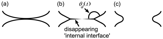
Figure 3: Sketch illustrating the scheme used in the interface formation/disappeance theory: the initial contact point (a) is followed by a fraction of the free surface being ‘trapped’ between the bulk phases, forming a gradually disappearing ‘internal interface’ (b), and, as the ‘internal interface’ disappears and the ‘contact angle’ $\theta_{d}$, being initially equal to $180^{\circ}$, relaxes to its ‘equilibrium’ value of $90^{\circ}$, the conventional mechanism takes over (c). The interface formation/disappearance model provides boundary conditions on interfaces, which are modelled as zero-thickness ‘surface phases’; these interfaces, including the ‘internal interface’ in (b), are shown as finite-width layers for graphical purposes only.

Applying the interface formation model to coalescence phenomena results in a new perspective on the problem. Instead of thinking of coalescence as the process by which one deformed body evolves, which is how equations (1) and (2) were derived, it is thought of as the process by which two drops evolve into a single entity. Specifically, just after the drops first meet, an internal interface divides them, which allows an angle to be sustained in the free surface, and the coalescence process is thought of as the time it takes for this internal divide between the two drops to disappear, and hence for the free surface to become smooth. A characteristic time of this process is the surface tension relaxation time, and, given that this parameter’s value is expected to be proportional to viscosity, it is likely that, for high viscosity fluids, such as the $58000$ mPa s silicon oil used in (paulsen12, ), direct experimental evidence for this model, in particular the angle in the free surface at a finite time after the drops first come into contact, may be possible to observe in the optical range.

The local asymptotic analysis carried out in (shik00, ; shik07, ) has shown that the singularities inherent in the conventional treatment of the early stage of coalescence are removed, but, to validate the theory experimentally, a global solution must be found. The obstacle here is that the interface formation model introduces a new class of problems where boundary conditions for the Navier-Stokes equations are themselves differential equations along a priori unknown interfaces, and this class of problems poses formidable difficulties even for numerical treatment. The decisive breakthrough in this direction has been made recently as a regular framework for computing this kind of problems has been developed(sprittles_jcp, ). This advance together with the development of the aforementioned novel experimental techniques, which can probe the coalescence process on the spatio-temporal scales well beyond the reach of previous studies, make a full comparison between theory and experiment possible for the first time.

II.6 Outline of the paper

The aim of this paper is to address whether the conventional model or the interface formation model are able to describe experimental results which give the bridge radius as a function of time over a range of viscosities. To do so, in Section III we present the problem formulations for both models and, notably, list the equations of interface formation, with a very brief description and references for detail. In Section IV, the computational tool, which was originally devised to describe dynamic wetting flows, is briefly described and references are given to the publications where detailed benchmarking and mesh-independence tests have been reported. In Section V, simulations from this code, for both low and high viscosity liquids, obtained using the conventional model, are shown to be in agreement with previous benchmark computational results. Besides validating the code, this allows us to consider the accuracy of the scaling laws proposed in various limits. Then, in Section VI, the predictions of both the conventional model and the interface formation model are compared to experiments conducted in both (thoroddsen05, ) and (paulsen11, ). This allows us to assess which of these models describes the underlying physics of the coalescence phenomenon. Next, in Section VII, a comparison is made to experiments in (paulsen11, ) over a range of viscosities, in order to ascertain how well the models are able to capture the observed drop behaviour. In subsections A and B of Section VIII, we propose a theory-guided test case which could potentially bring the differences between the two models’ predictions into the optical range. Concluding remarks in Section IX summarize the main results and point out some open issues for future research.

III Modelling of Coalescence Phenomena

Consider the axisymmetric coalescence of two drops whose motion takes place in the $(r,z)$-plane of a cylindrical coordinate system. The liquid is incompressible and Newtonian with constant density $\rho$ and viscosity $\mu$, and the drops are surrounded by an inviscid dynamically passive gas of a constant pressure $p_{g}$. To non-dimensionalize the system of equations for the bulk variables, we use the drop radius $R$ as the characteristic length scale; $U_{visc}=\sigma/\mu$ as the scale for velocities (so that $Ca=\mu U_{visc}/\sigma=1$), where $\sigma$ is the equilibrium surface tension of the free surface; $T_{visc}=R/U_{visc}=\mu R/\sigma$ as the time scale; and $\sigma/R$ as the scale for pressure. Then, the continuity and momentum balance equations take the form

$$\nabla\cdot\mathbf{u}=0,\qquad Re~{}\left[\dfrac{\partial\mathbf{u}}{\partial{t}}+\mathbf{u}\cdot\nabla\mathbf{u}\right]=-\nabla p+\nabla^{2}\mathbf{u}+Bo~{}\mathbf{g},$$ (3)

where $t$ is time, $\mathbf{u}$ and $p$ are the liquid’s velocity and pressure, and $\mathbf{g}$ is the gravitational force density, which in the nondimensional formulation is a unit vector in the negative $z$-direction. The non-dimensional parameters are the Reynolds number $Re=\rho\sigma R/\mu^{2}$ and the Bond number $Bo=\rho gR^{2}/\sigma$. To simplify the computations, we shall assume that gravitational forces are negligible $Bo=0$, so that, for two identical drops of radius $R$, the process can be regarded as symmetric with respect to the plane touching the two drops at the moment of their initial contact, and we can consider the flow in one drop, using the symmetry conditions at the symmetry plane $z=0$. The point in the $(r,z)$-plane at which the free surface meets the plane of symmetry will be referred to as the ‘contact line’, since, as we will show below, there is a certain analogy between the process of dynamic wetting and the coalescence phenomenon, where, in the present case, the drop (for definiteness, the one above $z=0$) ‘spreads’ over the plane of symmetry (see Figure 3). For the same reason, the angle $\theta_{d}$ between the free surface and the symmetry plane $z=0$ will be referred to as the ‘contact angle’, so that, in the analogy with dynamic wetting, the ‘equilibrium’ contact angle is $90^{\circ}$.

The effect of neglecting gravity is estimated in the Appendix, where we show that, as one would expect, gravity influences only the late stages of the drops’ evolution, i.e. the global geometry of the flow, where it is important whether the drops are spherical or hemispherical. In the present paper, we are interested primarily in the local process where coalescence as such takes place, and this process can be studied without taking gravity into account.

The boundary conditions to equations (3) will be given by two different models. First, we give the conventional model formulation routinely used for studying free-surface flows, and then we will present the interface formation model, which, until now, has not been used in full to describe this class of flows.

III.1 Conventional modelling

The standard boundary conditions used in fluid dynamics of free-surface flows are the kinematic condition, stating that the fluid particles forming the free surface stay on the free surface at all time, and the conditions of balance of tangential and normal forces acting on an element of the free surface from the two bulk phases and from the neighbouring surface elements:

$$\dfrac{\partial f}{\partial{t}}+\mathbf{u}\cdot\nabla f=0,$$ (4)

$$\mathbf{n}\cdot\left[\nabla\mathbf{u}+\left(\nabla\mathbf{u}\right)^{T}\right]\cdot\left(\mathbf{I}-\mathbf{n}\mathbf{n}\right)=\mathbf{0},$$ (5)

$$p_{g}-p+\mathbf{n}\cdot\left[\nabla\mathbf{u}+\left(\nabla\mathbf{u}\right)^{T}\right]\cdot\mathbf{n}=\nabla\cdot\mathbf{n}.$$ (6)

Here $f(r,z,t)=0$ describes the a priori unknown free surface, with the inward normal $\mathbf{n}=\nabla f/|\nabla f|$; $\mathbf{I}$ is the metric tensor of the coordinate system, so that the convolution of a vector with the tensor $(\mathbf{I}-\mathbf{n}\mathbf{n})$ extracts the component of this vector parallel to the surface with the normal $\mathbf{n}$ (in what follows, for brevity, we will mark these components with a subscript $\parallel$, so that $\mathbf{u}_{||}=\mathbf{u}\cdot(\mathbf{I}-\mathbf{n}\mathbf{n})$).

At the plane of symmetry $z=0$, one has the standard symmetry conditions of impermeability and zero tangential stress,

$$\mathbf{u}\cdot\mathbf{n}_{s}=0,~{}~{}~{}\mathbf{n}_{s}\cdot\left[\nabla\mathbf{u}+\left(\nabla\mathbf{u}\right)^{T}\right]\cdot\left(\mathbf{I}-\mathbf{n}_{s}\mathbf{n}_{s}\right)=\mathbf{0},$$ (7)

where $\mathbf{n}_{s}$ is the unit normal to the plane of symmetry. One also has the condition that the free surface is smooth, i.e. $\theta_{d}\equiv\pi/2$, or, in terms of the normals $\mathbf{n}$ and $\mathbf{n}_{s}$ to the free surface and the plane of symmetry, respectively, $\mathbf{n}\cdot\mathbf{n}_{s}=0$.

We will consider an axisymmetric flow, and on the axis of symmetry the standard impermeability and zero tangential stress condition apply:

$$\mathbf{u}\cdot\mathbf{n}_{a}=0,\qquad\mathbf{n}_{a}\cdot\left[\nabla\mathbf{u}+\left(\nabla\mathbf{u}\right)^{T}\right]\cdot(\mathbf{I}-\mathbf{n}_{a}\mathbf{n}_{a})=\mathbf{0},$$ (8)

where $\mathbf{n}_{a}$ is the unit normal to the axis of symmetry in the $(r,z)$-plane.

With regard to the overall drop geometry, there are two cases (Figure 2). In the case of the coalescence of free spherical drop, one needs the symmetry condition on the free-surface shape, namely that the free surface is smooth at the axis of symmetry,

$$\mathbf{n}\cdot\mathbf{n}_{a}=0,\quad\hbox{for}\quad f(0,z,t)=0,~{}~{}t\geq 0.$$ (9)

In the case of hemispherical drops pinned to the solid support, we need the condition that the coordinates of the free surface are prescribed where the free surface meets the solid:

$$f(1,1,t)=0\qquad(t\geq 0).$$ (10)

To complete the formulation, one needs the initial conditions, which we will discuss and specify below.

III.2 The interface formation/disappearance model

The interface formation/disappearance model formulates the boundary conditions that generalize (4)–(7) to account for situations in which the interfaces are forming or disappearing. In these cases, the interfaces have dynamic interfacial properties, and, in particular, the surface tension is no longer a constant; it varies as the interface is forming/disappearing, and this creates spatial gradients of the surface tension which give rise to the Marangoni flow in the bulk. The equations of the interface formation model consider interfaces as two-dimensional ‘surface phases’ characterized, besides the surface tension, by the surface density $\rho^{s}$ and the surface velocity $\mathbf{v}^{s}$ with which the surface density is transported. The normal to the interface component of $\mathbf{v}^{s}$ can differ from the normal component of the bulk velocity $\mathbf{u}$ evaluated at the interface as there can be mass exchange between the surface and bulk phases.

The details of the interface formation model can be found elsewhere(shik07, ), so that here we will give the necessary equations in the dimensionless form, using as characteristic scales for $\rho^{s}$, $\mathbf{v}^{s}$ and $\sigma$ the surface density corresponding to zero surface tension $\rho^{s}_{(0)}$, the same velocity scale as used in the bulk $\sigma/\mu$, and the equilibrium surface tension of the liquid-gas interface $\sigma=\sigma_{1e}$, respectively. In what follows, subscripts 1 and 2 will refer, respectively, to the surface variables on the free surface and on the plane of symmetry $z=0$, which will be regarded as a gradually disappearing ‘internal interface’ trapped between the two coalescing drops as they are pressed against each other. Notably, the plane of symmetry $z=0$ actually cuts the internal interface into two symmetric halves and we consider the upper half of this interface which, for brevity, is referred to as the ‘internal interface’.

On the liquid-gas free surface, we have

$$\dfrac{\partial f}{\partial{t}}+\mathbf{v}^{s}_{1}\cdot\nabla f=0,$$ (11)

$$p_{g}-p+\mathbf{n}\cdot\left[\nabla\mathbf{u}+\left(\nabla\mathbf{u}\right)^{T}\right]\cdot\mathbf{n}=\sigma_{1}\nabla\cdot\mathbf{n},$$ (12)

$$\mathbf{n}\cdot\left[\nabla\mathbf{u}+\left(\nabla\mathbf{u}\right)^{T}\right]\cdot\left(\mathbf{I}-\mathbf{n}\mathbf{n}\right)+\nabla\sigma_{1}=\mathbf{0},$$ (13)

$$\left(\mathbf{u}-\mathbf{v}^{s}_{1}\right)\cdot\mathbf{n}=Q\left(\rho^{s}_{1}-\rho^{s}_{1e}\right),$$ (14)

$$\epsilon\left[\dfrac{\partial\rho^{s}_{1}}{\partial{t}}+\nabla\cdot\left(\rho^{s}_{1}\mathbf{v}^{s}_{1}\right)\right]=-\left(\rho^{s}_{1}-\rho^{s}_{1e}\right),$$ (15)

$$4\bar{\beta}\left(\mathbf{v}^{s}_{1||}-\mathbf{u}_{||}\right)=\left(1+4A\right)\nabla\sigma_{1},$$ (16)

$$\sigma_{1}=\lambda(1-\rho^{s}_{1}),$$ (17)

where the following nondimensional parameters have been introduced: $Q=\rho^{s}_{(0)}/(\rho\sigma\tau_{\mu})$, $\epsilon=\sigma\tau_{\mu}/R$, $\bar{\beta}=\beta R/\mu$, $A=\alpha\beta$, $\rho^{s}_{1e}=(\rho^{s}_{1e})_{dim}/\rho^{s}_{(0)}$, $\lambda=\gamma\rho^{s}_{(0)}/\sigma_{1e}$. Here, we have used the experimentally ascertained result (blake02, ) that, for a class of fluids commonly used in experiments, the characteristic relaxation time of the interface $\tau$ is linearly proportional to the liquid’s viscosity, with coefficient of proportionality $\tau_{\mu}$, so that $\tau=\tau_{\mu}\mu$.

Our assumption of symmetry between the two coalescing drops means that the position of the ‘trapped’ ‘internal interface’ is known a priori, so that the normal stress condition, which in the general case is used to find the interface’s shape, is not required, and we have the following equations:

$$\mathbf{v}^{s}_{2}\cdot\mathbf{n}=0,$$ (18)

$$\mathbf{n}\cdot\left[\nabla\mathbf{u}+\left(\nabla\mathbf{u}\right)^{T}\right]\cdot\left(\mathbf{I}-\mathbf{n}\mathbf{n}\right)+\nabla\sigma_{2}=\mathbf{0}$$ (19)

$$\left(\mathbf{u}-\mathbf{v}^{s}_{2}\right)\cdot\mathbf{n}=Q\left(\rho^{s}_{2}-1\right),\qquad\epsilon\left[\dfrac{\partial\rho^{s}_{2}}{\partial{t}}+\nabla\cdot\left(\rho^{s}_{2}\mathbf{v}^{s}_{2}\right)\right]=-\left(\rho^{s}_{2}-1\right),$$ (20)

$$4\bar{\beta}\left(\mathbf{v}^{s}_{2||}-\mathbf{u}_{||}\right)=\left(1+4A\right)\nabla\sigma_{2},\qquad\sigma_{2}=\lambda(1-\rho^{s}_{2}).$$ (21)

As one can see, these equations are the same as (11)–(17) with $\rho^{s}_{1e}=1$. This means that in equilibrium the ‘internal interface’ vanishes, no longer having the surface tension and mass exchange with the ‘bulk’, which are the only factors that distinguish it as a special ‘surface phase’.

Although the boundary conditions of the interface formation model have been explained in detail elsewhere (shik07, ), it seems reasonable to briefly recapitulate their physical meaning. On the free surface, besides the standard kinematic condition (11) and also standard conditions on the normal and tangential stress (12) and (13), where the latter includes the Marangoni effect due to the (potentially) spatially nonuniform surface tension, one has the conditions describing the mass exchange between the interface and the bulk (14), (15), the equation describing how the difference between the tangential components of the surface velocity and the bulk velocity evaluated at the interface is related to the surface tension gradient (16), and the surface equation of state (17). The conditions on the internal interface are a simplification of the conditions on the free surface due to the fact that the shape of this interface is known ($z=0$), so that the normal-stress boundary condition, which applied to the entire internal interface, i.e. the upper and lower halves put together, is automatically satisfied, due to the symmetry of the problem with respect to the $z=0$ plane, and is hence not needed, and the kinematic boundary condition simplifies to (18). In the case of a problem not symmetric with respect to the plane $z=0$ both of these conditions should be used in their full form.

Estimates for the phenomenological material constants $\alpha$, $\beta$, $\gamma$, $\rho^{s}_{(0)}$ and $\tau$ have been obtained by comparing the theory to experiments in dynamic wetting, e.g. in (blake02, ), but could equally well have been taken from any other process involving the formation or disappearance of interfaces.

Boundary conditions (11)–(21) are themselves differential equations along the interfaces and therefore are in need of boundary conditions at the boundaries of the interfaces, i.e. at the contact line where the free surface meets the internal interface, at the axis of symmetry (if free drops are considered) or the solid boundary (in the case of pinned drops). At the contact line, one has the continuity of surface mass flux and balance of horizontal projection of forces due to surface tensions acting on the contact line:

$$\rho^{s}_{1}\left(\mathbf{v}^{s}_{1||}-\mathbf{U}_{c}\right)\cdot\mathbf{m}_{1}+\rho^{s}_{2}\left(\mathbf{v}^{s}_{2||}-\mathbf{U}_{c}\right)\cdot\mathbf{m}_{2}=0,$$

$$\sigma_{2}+\sigma_{1}\cos\theta_{d}=0.$$ (22)

Here $\mathbf{m}_{i}$ are the unit vectors normal to the contact line and inwardly tangential to the free surface ($i=1$) and the plane of symmetry ($i=2$); $\mathbf{U}_{c}$ is the velocity of the contact line (which is, obviously, directed horizontally). Equation (22) is the well-known Young’s equation(young05, ) that introduces and determines the contact angle in the processes of dynamic wetting. The present model essentially considers coalescence as the process where the two drops ‘spread’ over their common boundary which gradually loses its ‘surface’ properties, and the contact angle tends to its ‘equilibrium value’ of $90^{\circ}$, where one will have the familiar smooth free surface, whose evolution can be described by the conventional model.

For the bulk velocity $\mathbf{u}$ one again has (8) on the axis of symmetry and conditions (9) or (10) for the free surface. Additionally, at the axis of symmetry (in the case of free drops) or at the solid surface (in the case of the drops pinned to the solid), the boundary condition is the absence of a surface mass source/sink, so that one has

$$\mathbf{v}^{s}\cdot\mathbf{k}=0,$$ (23)

where $\mathbf{k}=\mathbf{n}_{a}$ for the free drops and a unit vector tangential to the free surface in the case of pinned drops.

Notably, at leading order in the limit $\epsilon\rightarrow 0$, which is associated with taking to zero the ratio of the characteristic length scale of interface formation $U\tau$ $(=\sigma\tau_{\mu}$) to that of the bulk flow $R$, the interface formation model reduces to the standard model. In simple terms: one can see that for $\epsilon=0$ equation (14) and the second equation in (20) immediately give $\rho^{s}_{1}=\rho^{s}_{1e}$ and $\rho^{s}_{2}=1$, i.e. the interfaces are in equilibrium, so that $\sigma_{1}=1$ and $\sigma_{2}=0$, which results in the standard stress-balance and kinematic equations on the free surface, the absence of an internal interface, and, from the Young equation (22), an instantaneously smooth free surface $\theta_{d}=90^{\circ}$.

III.3 Initial Conditions

The initial conditions for the conventional model and the interface formation model are essentially different as they represent how the two models view the onset of coalescence. In the conventional model, it is assumed that, after coming into contact, the two drops instantaneously produce a smooth free surface, i.e. they immediately coalesce and round the corner enforced by the drops’ initial configuration at the moment of touching. Therefore, besides prescribing the fluid’s initial velocity, which we will assume to be zero,

$$\mathbf{u}=\mathbf{0}\qquad\hbox{at }t=0,$$ (24)

we need to specify the initial shape as having, near the origin, a tiny bridge whose free surface crosses the plane of symmetry at the right angle. The free-surface shape far away from the origin (i.e. from the point of the initial contact) is the undisturbed spherical (or hemispherical) drop. The initial radius of the bridge $r_{min}$ is a parameter whose influence is to be investigated, although it is known a priori that the limit $r_{min}\rightarrow 0$ gives rise to a singularity. For both a spherical and a hemispherical drop, the free surface below the drop’s centre is conventionally prescribed as the one given by Hopper’s solution (hopper84, ), that is the analytic two-dimensional solution for Stokes flow, whose parametric form is

$$r(\theta)=\sqrt{2}\left[(1-m^{2})(1+m^{2})^{-1/2}(1+2m\cos\left(2\theta\right)+m^{2})^{-1}\right](1+m)\cos\theta,$$

$$z(\theta)=\sqrt{2}\left[(1-m^{2})(1+m^{2})^{-1/2}(1+2m\cos\left(2\theta\right)+m^{2})^{-1}\right](1-m)\sin\theta,$$ (25)

for $0<\theta<\theta_{u}$, where $m$ is chosen so that $r(0)=r_{min}$ and $\theta_{u}$ is chosen so that $r(\theta_{u})=z(\theta_{u})=1$. Notably, for $r_{min}\to 0$ we have $m\to 1$ and $r^{2}+(z-1)^{2}=1$, i.e. the drop’s profile is a semicircle of unit radius which touches the plane of symmetry at the origin.

The interface formation model does not presume an instant coalescence, so that, after the two drops touch and then establish a nonzero area of contact, (a) there is still an internal interface between them, and hence coalescence as the formation of a single body of fluid is only starting, and (b) the free surface is not smooth, as the initial angle of contact of $180^{\circ}$ is only starting its evolution towards $90^{\circ}$, i.e. a smooth interface. For both a spherical and a hemispherical drop, the free surface below the drop’s centre can be prescribed as

$$(r-r_{min})^{2}+(z-z_{c})^{2}=z_{c}^{2},$$ (26)

where $z_{c}=\hbox{$\frac{1}{2}$}(1+(1-r_{min})^{2})/2$, so that if there is no base, i.e. $r_{min}=0$, one has $z_{c}=1$, i.e. $r^{2}+(z-1)^{2}=1$, which is a circle of radius $1$ centred at $(0,1)$ that coincides with the shape obtained from (25) in the same limit. Importantly, for the interface formation model the limit $r_{min}\rightarrow 0$ does not give rise to a singularity.

In addition to the free-surface shape given by (26) and the flow field in the bulk, by (24), we need to specify the initial state of the interfaces, which will be given by

$$\rho^{s}_{1}=\rho^{s}_{2}=\rho^{s}_{1e},\qquad(t=0),$$ (27)

These conditions in (27) describe the fact that (a) the free surface is initially in equilibrium, and (b) the part of the free surface that has been sandwiched between the two drops and becomes an ‘internal’ interface initially possesses the equilibrium properties of the free-surface, since it can equilibrate to its new environment in a finite time. Then, for $t>0$, the internal interface will start to relax towards its equilibrium state, which in turn will drive the free surface away from its initial (equilibrium) state, so that in the early stages of the coalescence phenomenon both interface will be out of equilibrium and will, in particular, deviate from the initial values given in (27). Notably, the assumption that all the interfaces are unchanged from their pre-coalescence state is consistent with an initial contact angle of $\theta_{d}=180^{\circ}$, which follows from the Young equation (22) for $\sigma_{1}=\sigma_{2}=1$, i.e. when $\rho^{s}_{1}=\rho^{s}_{2}=\rho^{s}_{1e}$.

IV A Computational Framework for Free-Surface Flows with Dynamic Interfacial Effects

A finite-element-based computational platform for simulating free-surface flows with dynamic interfacial effects has been developed in (sprittles11c, ; sprittles_jcp, ) and originally applied to microfluidic dynamic wetting processes, which are the most complex case of these flows. The ability of the developed framework to simulate flows involving strong deformations of a drop has already been confirmed in (sprittles_pof, ), where the predictions of the code are shown to be in excellent agreement with previous literature for the benchmark test-case of a freely oscillating liquid drop. In (sprittles_jcp, ), the interface formation model was incorporated in full into the framework and allowed the simulation of microfluidic phenomena such as capillary rise, showing excellent agreement with experiments, and, in (sprittles_pof, ), the impact and spreading of microdrops on surfaces of varying wettability. The exposition in (sprittles_jcp, ) together with the preceding paper (sprittles11c, ) provide a detailed step-by-step guide to the development of the code, allowing one to reproduce all results, as well as curves for benchmark calculations and a demonstration of the platform’s capabilities. Therefore, here it is necessary only to point out a few aspects of the computations.

The code is based on the finite element method and uses an arbitrary Lagrangian-Eulerian mesh design (kistler83, ; heil04, ; wilson06, ) to allow the free surface to be accurately represented whilst bulk nodes remain free to move. For the drop geometry, the mesh is based on the bipolar coordinate system, and is graded to allow for extremely small elements near the contact line and progressively larger elements in the bulk of the liquid. This ensures that all the physically-determined smallest scales near the contact line are well resolved whilst the problem is still computationally tractable. The conditions on the mesh needed to resolve the scales associated with the interface formation in dynamic wetting problems are given in (sprittles_jcp, ). However, for the coalescence phenomenon, even smaller elements are required to capture the free-surface shape associated with the conventional model. Indeed, the initial free-surface shape given by (25) requires that the free surface bends near the plane of symmetry $z=0$ to meet this boundary perpendicularly at $r=r_{min}$. The radius of curvature of the free surface where it meets $z=0$ is of $O(r_{min}^{3})$ and for $r_{min}=10^{-4}$, used in our computations, one has the radius of curvature $\sim 10^{-12}$, i.e. extremely small and many orders of magnitude smaller than the length scales associated with the interface formation dynamics. Here the model is used beyond its area of applicability, as in the derivation of the capillary pressure due to the free-surface curvature it is assumed that the radius of curvature is much larger than the physical thickness of the interface, which is modelled as a geometric surface of zero thickness. However, the conventional model dictates that this is the scale which needs to be resolved, so that in order to provide mesh-independent solutions from this model the elements near the contact line have to be exceptionally small. On such scales, it is somewhat surprising that, even with the huge amount of care taken, we have been able to produce mesh-independent converged solutions. Any further reduction of $r_{min}$ for the conventional model has been seen to be impossible. To capture dynamics on this scale would require one to ‘zoom in’ on the coalescence event, which will initially be isolated from the global dynamics, and then stitch this solution to a global result at a later time, i.e. essentially to mimic numerically the technique of matched asymptotic expansions.

The result of our spatial discretization is a system of non-linear differential algebraic equations of index two (lotstedt86, ) which are solved using the second-order backward differentiation formula, whose application to the Navier-Stokes equations is described in detail in (gresho2, ), using a time step which automatically adapts during a simulation to capture the appropriate temporal scale at that instant.

V Benchmark Simulations

In order to compare our computations for the conventional model to the numerical results presented in (paulsen12, ), we consider the coalescence of liquid spheres of radius $R=1$ mm, density $\rho=970$ kg m^-3, surface tension $\sigma_{1e}=20$ mN m^-1 for viscosities $\mu=1$ mPa s and $\mu=58000$ mPa s. For these parameters, the Reynolds numbers are $Re=1.9\times 10^{4}$ and $Re=5.8\times 10^{-6}$, respectively, which allows us to investigate both the inertia-dominated and viscosity-dominated regimes.

Before doing so, we must make some comments regarding the computation of the very initial stages of coalescence. In particular, in some simulations, for both the conventional and the interface formation models, we have observed the tendency towards the formation of toroidal bubbles, as the disturbance to the free surface, initiated by the coalescence event, leads to capillary waves which come into contact with the plane of symmetry (i.e., for the two drops, into contact with each other), in front of the propagating contact line. This effect is essentially the same as the one reported in (duchemin03, ; oguz89, ) and in our computations only occurs for low-viscosity liquids. It is particularly severe for the conventional model’s computations, where the contact angle variation, from $180^{\circ}$ at the moment of touching to $90^{\circ}$ when the computations start, creates a greater disturbance of the initial (equilibrium) free-surface shape and hence causes larger free surface waves than those produced by the interface formation model when the contact line begins to move. Computationally, as only one drop in this symmetric system is considered, there is nothing to stop the free surface piercing the $z=0$ plane of symmetry, and in Figure 4 the dashed curves show the profiles obtained if no special treatment is provided, for computations of the $Re=1.9\times 10^{4}$ liquid using the conventional model, i.e. the worst case scenario.

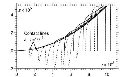
Figure 4: Free-surface profiles obtained using the conventional model for the coalescence of two free drops with $Re=1.9\times 10^{4}$ at intervals of $\triangle t=10^{-3}$. Dashed lines: the computed solution in which the free surface is allowed to freely pierce the plane of symmetry ($z=0$). Solid lines: solution when the free surface is prevented, as it is henceforth, from crossing the symmetry plane.

Physically, if the two free surfaces reconnect instantaneously upon coming into contact, i.e. begin to coalesce, then the simulation should be continued with a trapped toroidal bubble and a multiply-connected domain. However, as the capillary waves propagating along the free surfaces of the two drops try to reconnect, the viscosity of the gas in the narrow gap between them can no longer be neglected since the gas will be acting as a lubricant preventing the free surfaces from touching. In any case, at present, accounting for the dynamics of a trail of toroidal bubbles deposited behind an advancing free surface is beyond developed computational methods. An alternative approach, is to assume that, as the free surfaces of the two drops try to touch ahead of the contact line, they do not coalesce immediately, i.e. remain free surfaces for the short time that they are in contact, as then the capillary waves propagate further and these free surfaces separate. This approach may well mimic the reality, as one has to drain the air film between the two converging surfaces before coalescence can occur, which could explain why there is yet to be any experimental validation of the existence of the toroidal bubbles. The profiles obtained using this approach are shown as the solid lines in Figure 4, and it is this approach that we use henceforth in the situations where the free surface touches or tries to pierce the plane of symmetry.

In Figure 5, one can see that the difference between the two approaches, i.e. between allowing the free surface to freely pierce the plane of symmetry and using the plane of symmetry as a geometric constraint, is visible but small, with the second approach (curve 1b), where the free surface is unable to pass through the symmetry plane, predicting a slightly faster evolution of the bridge radius than when the penetration of the plane is allowed (curve 1a). This phenomenon clearly deserves more attention, and the development of more advanced computational techniques, but in what follows we use the method proposed above and note that the specific treatment does not appear to have a significant influence on the bridge radius, certainly compared to the error bars in the experiments shown in Section VI (see for example Figure 14) and only affects the lowest viscosity liquid drops.

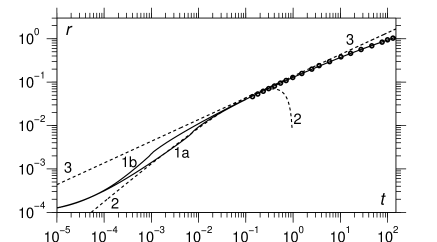
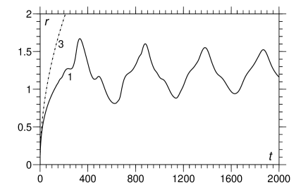
Figure 5: Bridge radius as a function of time obtained using the conventional model and scaling laws (1) and (2). Curve 1a: the free surface is allowed to pierce the plane of symmetry; curve 1b: simulations where piercing of the plane of symmetry was not allowed; curve 2: best fit ($C_{visc}=0.19$) of the scaling law (1); curve 3: the inviscid scaling law (2) with $C_{inert}=1.62$; circles: the numerical solution obtained in (paulsen12, ) for the same problem. After the initial stages curves 1a and 1b are graphically indistinguishable and so the label curve 1 is used.

The $\log$-$\log$ plot in Figure 5 shows the radius of the liquid bridge connecting the two coalescing drops as a function of time. Henceforth, $r$ refers to the radius of the free surface at the plane of symmetry, i.e. $r=r(0,t)$. The curves shown in Figure 5 have been computed using either of the two approaches to deal with the capillary waves piercing through the plane of symmetry: both curves 1a and 1b are graphically indistinguishable from the corresponding numerical results obtained in (paulsen12, ), so that circles had to be used to highlight the region, roughly $0.1<t<100$, for which a comparison was available.

Our results also give an opportunity to compare the full numerical solution we obtained to the scaling laws given by equations (1) and (2) described in Section II.2. As one can see in Figure 5, both scaling laws, (1) and (2), provide a good approximation of the conventional model’s solution over a considerable period of time. As expected, the viscosity-versus-capillarity scaling law (curve 2), with $C_{visc}=0.19$ in equation (1), provides a good approximation for early time, until roughly $t=0.1$. The inertia-versus-capillarity scaling law (curve 3), with $C_{inert}=1.62$ in equation (2) taken from (duchemin03, ), despite being used well outside its limits of applicability, agrees fairly well with our numerical solution from roughly $t\approx 0.1$ until approximately $t\approx 10$, at which point the (non-local) influence of the drop’s overall geometry becomes pronounced.

Of particular interest is that our simulations show the $r\sim t\ln t$ behaviour predicted in (eggers99, ), which, as far as we are aware, has never previously been observed in either experiments or simulations. In (eggers99, ), it is claimed that the viscosity-versus-capillarity scaling law is only valid when the Reynolds number $Re_{r}$ based on the bridge radius is less than one, i.e. $Re_{r}\equiv r\,Re<1$, which corresponds to $r<10^{-4}$ for our values of parameters. However, we observe that the scaling law approximates the actual solution up until almost $r=10^{-1}$, i.e. well outside its apparent limits of applicability. This is in agreement with the conclusions in (paulsen11, ), where it is claimed that, to ascertain the limits of applicability of the scaling law, one should use the Reynolds number $Re_{h}$ based on the undisturbed height of the free surface at a given radius, as opposed to the bridge radius itself. Given that $h\propto r^{2}$, we have the condition $Re_{h}=r^{2}Re<1$, which suggests that the scaling law is valid until $r<10^{-2}$, which is far closer to what we see. The above regime is followed by the inertial one after which something close to a $t^{1/2}$ scaling is observed.

In Figure 6, we show the results obtained using the conventional model for the global dynamics of the coalescence of low-viscosity ($Re=1.9\times 10^{4}$) spherical drops, as those considered in (basaran92, ). In this figure, we use the Cartesian $x$-coordinate instead of $r$ to give the full profile of the drops rather than just a half of it ($r\geq 0$). As one can see from Figure 5, as well as from the shape of the free surface in the last image in Figure 6 at $t=550$, the free surface continues to evolve for $t>550$, but this period is concerned with the free oscillation of a single liquid drop (see for example (basaran92, )), as opposed to the coalescence event which we are interested in here.

(a) $t=0$

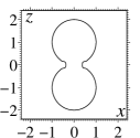
(b) $t=10$

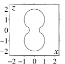
(c) $t=20$

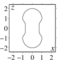
(d) $t=50$

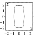
(e) $t=100$

(f) $t=150$

(g) $t=200$

(h) $t=250$

(i) $t=300$

(j) $t=350$

(k) $t=450$

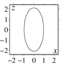
(l) $t=550$

Figure 6: Coalescence of two low-viscosity free liquid drops with $Re=1.9\times 10^{4}$.

The coalescence of the two high viscosity drops ($Re=5.8\times 10^{-6}$) is shown in Figure 7, where one can observe that, as one would expect, the drops coalesce without any oscillations. The $\log$-$\log$ plot in Figure 8 confirms that our code is giving results in agreement with previous computations that used the conventional model (paulsen12, ). This has been tested for both $r_{min}=10^{-4}$, curve 1a, as well as $r_{min}=10^{-3}$, curve 1b, and we can see that both curves converge well before reaching the circles which correspond to the results of (paulsen12, ). It is interesting to note that the curves converge on to curve 2 obtained from the viscosity-versus-capillarity scaling law, equation (1) with $C_{visc}=0.4$, after a time of $O(r_{min})$, i.e. the effect of the finite initial radius is lost after a (dimensionless) time $r_{min}$, which is generally very short in the cases we consider for the conventional model. Our estimate above, based on the extended period in which the scaling law held for a low viscosity fluid, suggested that this law will be valid until $Re_{h}=r^{2}Re<1$, which in this case gives $r<10^{2}$, i.e. for the entire period of motion. This cannot be the case as the scaling law blows up before reaching such radii, see Figure 7, and in fact we see once again that the scaling law agrees with the simulation up until almost $r=t=10^{-1}$. Notably, the $t\ln t$ behaviour approximates the simulation better than the best linear fit, curve 3, in contrast to experimental results (thoroddsen05, ; aarts05, ) which suggest that the linear fit is a better one. No $t^{1/2}$ scaling, as predicted by the inertia-versus-capillarity scaling law, is seen, as one would expect, and we have therefore omitted this case from the plot.

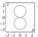
(a) $t=0$

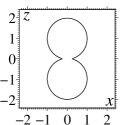
(b) $t=0.2$

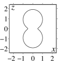
(c) $t=0.5$

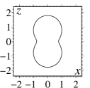
(d) $t=1$

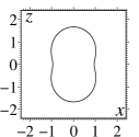
(e) $t=1.5$

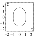
(f) $t=2$

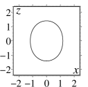
(g) $t=3$

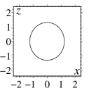
(h) $t=4.5$

Figure 7: Coalescence of two high viscosity free liquid drops with $Re=5.8\times 10^{-6}$.

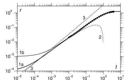
Figure 8: Bridge radius as a function of time obtained using the conventional model and scaling laws (1) and (2). Curve 1a: $r_{min}=10^{-4}$; curve 1b: $r_{min}=10^{-3}$; curve 2: best fit ($C_{visc}=0.4$) of the scaling law (1); curve 3: best fit linear curve ($r=3.5t$); circles: the numerical solution obtained in (paulsen12, ) for the same problem.

Having confirmed that, for the conventional model, our framework is giving results that are in agreement with previous studies into coalescence, and having used this model to study the limitations of the scaling laws proposed in the literature, we can now turn to a direct comparison of the two theories, the conventional model and the interface formation model, to recently published experimental data.

VI Comparison of different models to experiment

In this section, we will compare the predictions of both the conventional model and the interface formation model with experiments reported in (thoroddsen05, ) and (paulsen11, ). In both experimental setups, drops are formed from two nozzles and slowly brought together until coalescence occurs. In what follows, we will initially consider the drops to be hemispheres of radius $R=2$ mm, pinned at the nozzle edge from which they emanate (see Figure 2). In the Appendix, the influence of gravity and of the far-field flow geometry are quantified and shown to be negligible for the initial stages of coalescence which we are interested in, so that, for example, altering the length of the capillary, or its inlet conditions will have no influence on our forthcoming conclusions.

As in the experiments in (paulsen11, ), we consider the dynamics of water-glycerol mixtures of density $\rho=1200$ kg m^-3 and surface tension with air of $\sigma_{1e}=65$ mN m^-1 for a range of viscosities $\mu=3.3,~{}48,~{}230$ mPa s, which are chosen as some of the cases where $\sigma_{1e}$ and $\rho$ vary least, giving $Re=1.4\times 10^{4},~{}68,~{}2.9$. The dependence of the interface formation model’s parameters on surface tension and drop radius are

$$Q=q_{1}\sigma^{-1},\quad\epsilon=q_{2}\sigma R^{-1},\quad\bar{\beta}=q_{3}R,\quad A=1,\quad\rho^{s}_{1e}=0.6,\quad\lambda=(1-\rho^{s}_{1e})^{-1},$$ (28)

and estimates for the dimensional constants, the $q$’s, for water-glycerol mixtures have been obtained from experiments on dynamic wetting(blake02, ) as $q_{1}=3\times 10^{-4}$ N m^-1, $q_{2}=7\times 10^{-6}$ N^-1 m² and $q_{3}=5\times 10^{8}$ m^-1.

Fortuitously, at the highest viscosity we can also compare our results to those in (thoroddsen05, ) where the same liquid mixture was used . Furthermore, at the highest viscosity there are no complications from toroidal bubbles and the viscosity ratio between the liquid and surrounding air is large, so that all influences on the coalescence dynamics additional to those considered, such as the dynamics of the gas, are negligible. In other words, this is the perfect test case for a comparison between the conventional model, the interface formation model and experimental data.

Notably, in contrast to the coalescence of two free liquid drops, where the final stage of the process is one spherical drop of the combined volume, the equilibrium shape of the two coalescing hemispheres pinned at the capillary edge is no longer analytically calculable. So, a simple code was written to solve for the static equilibrium shapes of the drops using the approach outlined in (fordham48, ). In Figure 9, snapshots from the coalescence event are shown and, critically, it can be seen that our simulations predict the correct equilibrium shape. On this scale, there is seemingly little difference between the two models’ predictions, as one would expect given that the two equilibrium shapes are the same. To access verifiable differences between the models and to compare the results with the experiments, we now consider the initial stages of the coalescence process.

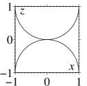
(a) t=0

(b) t=0.5

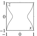
(c) t=1

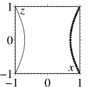
(d) t=4

Figure 9: Coalescence of two pinned hemispheres with $Re=2.9$, with the independently obtained equilibrium position shown by a dashed line.

In Figure 10, we show the free-surface profiles obtained from our simulations using the two different models. In the initial stages of coalescence, one can see that the conventional model (upper curves) predicts a faster motion than that given by the interface formation model (lower curves). As can also be seen from Figure 10, the contact angle predicted by the interface formation model takes a finite time to evolve and establish the smooth free surface. This time period is associated with $\theta_{d}>90^{\circ}$, and only towards the end of the evolution of the free surface shown in the figure the contact angle approaches $90^{\circ}$, indicating that the physics embodied in the conventional model can take over. This gradual evolution of the contact angle results in a slower motion in the initial stages than that predicted by the conventional model where, as we know, the initial velocity, driven by a region of extremely high curvature and hence high capillary pressure, is huge. As we shall see, this difference between the models’ predictions will reduce as time from the onset of the process passes and the two drops evolve towards the same equilibrium position. Therefore, it is the initial stages of the evolution, such as those shown in Figure 10, that the discrepancies between theory and experiment will be most easily picked up.

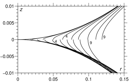
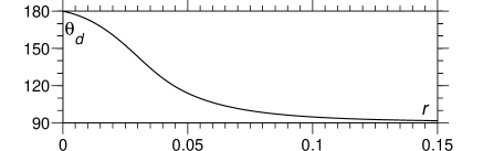
Figure 10: Top: Comparison of the free surface profiles for the initial stages of coalescence for the highest viscosity fluid ($Re=2.9$) obtained using the conventional model (upper curves) and the interface formation model (lower curves). Snapshots are taken every $\triangle t=10^{-2}$ so that curves 4 are at $t=0.04$ and curves 9 are at $t=0.09$. Bottom: Contact angle at which the free surface meets the plane of symmetry for the interface formation model.

The bridge radius as a function of time for the highest viscosity ($Re=2.9$) is given in Figure 11, which shows a comparison between the two models’ predictions and the experimental data from in (thoroddsen05, ) and (paulsen11, ). In particular, the initial time of coalescence in the optical experiment of (thoroddsen05, ), which is known to be uncertain, is chosen such that one has an overlap with the data of the electrical experiments of (paulsen11, ), where the initial time was more accurately determined.

It is immediately apparent that the bridge radius predicted by the conventional model overshoots the experimental values of both studies for a considerable amount of time. For the interface formation model, using parameters (28), we obtain curve $3$. Alteration of any of these parameters is seen to result in a worse agreement with experiment with the exception of the parameter $\rho^{s}_{1e}$, which is the equilibrium surface density on the free surface. Decreasing its value to $\rho^{s}_{1e}=0.2$ gives curve $2$, which goes through all of the error bars and data points except for the very first one. As one would expect, all the curves coincide as the equilibrium position is approached and both agree with the optical experiments in these final stages of evolution.

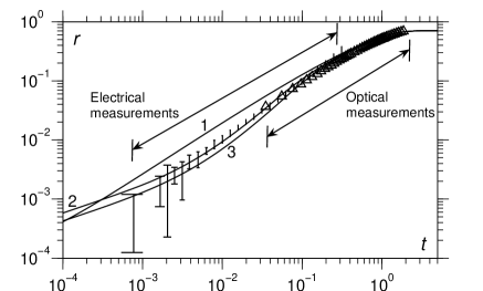
Figure 11: Bridge radius as a function of time for viscosity $\mu=220$ mPa s ($Re=2.9$) obtained using different models compared to experiments from (paulsen11, ) (with error bars) and Figure 17b in (thoroddsen05, ) (triangles). Curve 1: the conventional model; curve 2: the interface formation model with $\rho^{s}_{1e}=0.2$ and other parameters from (28); curve 3: the interface formation model with parameters from (28).

In Figure 12, the distributions of the surface tensions along both the free surface and the internal interface are shown at different instances through the simulation. Notably, although the free surface is in equilibrium ($\sigma_{1}=1$) both initially and at the end of the coalescence process when one has a single body of fluid confined by a smooth free surface, as the interface formation dynamics unfolds ($t>0$), the surface tension distribution near the contact line becomes driven away from equilibrium, with, in particular, $\sigma_{1}=0.63$ at the contact line when $t=10^{-2}$, which is not far away from its minimum value of $\sigma_{1}=0.61$ reached at $t=0.017$. As can be seen from Figure 10, it is at this time that the contact angle rapidly decreases from its initial value of $\theta_{d}=180^{\circ}$, imposed by the initial conditions, to its equilibrium value of $\theta_{d}=90^{\circ}$, which it is close to achieving by $t=10^{-1}$. Consequently, the behaviour of $\sigma_{1}$ is non-monotonic in time, with an initial decrease in its distribution near the contact line followed by a relaxation back towards its equilibrium state. As one would expect, when there is a separation of length scales between the drop radius and the length scale of interface formation, the surface tension on the free surface far away from the contact line, roughly $s>10^{-2}$, remains in its equilibrium state throughout the coalescence process. However, the internal interface, which has length $s=10^{-4}$ at the start of the simulation, is comparable with the length scale on which the interface formation model acts, and hence, as one can see from Figure 12, it takes a finite time for the interface to form, and for this interface there is no ‘far-field’ where the interface is in equilibrium until around $t=10^{-1}$, at which point the length of the internal interface has increased significantly.

Figure 12: Evolution of the surface tension distributions along the free surface, $\sigma_{1}$, and internal interface, $\sigma_{2}$, as a function of distance from the contact line $s$ at times 0: $t=0$; 1: $t=10^{-5}$; 2: $t=10^{-4}$; 3: $t=10^{-3}$; 4: $t=10^{-2}$; 5: $t=10^{-1}$; 6: $t=1$, for the highest viscosity fluid ($Re=2.9$), obtained using the interface formation model.

In our comparison of the two models with experiments, the following two aspects can be highlighted. Firstly, it is apparent that the conventional model considerably overpredicts the speed at which coalescence occurs. This is consistent with the fact that this model introduces unphysical singular velocities at the start of the process, as the cusp in the free surface shape is instantaneously rounded. In our computations, this unphysicality is moderated by our use of the zero velocity initial condition (24) but the influence of this initial condition quickly dies out, and one ends up with the rate of the widening of the bridge connecting the two drops well above what is actually observed. In contrast, the interface formation model predicts that the angle at which the free surface meets the plane of symmetry will relax from its initial value of $180^{\circ}$ to its eventual value of $90^{\circ}$ gradually, over some characteristic time scale. In Figure 10, this behaviour is observed, where the angle remains high for a considerable amount of time, being greater than $170^{\circ}$ until $t=10^{-2}$, gradually relaxing to $90^{\circ}$ and reaching this value at around $t=10^{-1}$. What is unexpected, is that the non-dimensional relaxation time of the interface $\tau_{nd}=\tau/(R\mu/\sigma)=\tau_{\mu}\sigma/R=O(10^{-4})$ is not a good approximation for the period in which the interface is out of equilibrium, i.e. the free surface is not smooth; in fact, the time scale over which interface formation acts is much larger, which suggests that the influence of these effects could extend outside the parameter space previously identified.

The second aspect, which is perhaps more important, is the trends observed in experiments and predicted by the two models. In experiment and in what the interface formation model predicts, one can see what looks like two different regimes, roughly corresponding, coincidentally, to the ranges of the electric and optical measurements, whereas the conventional model describes the process as ‘more of the same’, with no qualitative difference between the early stages of the process and the subsequent dynamics. This is consistent with the fact that the conventional model assumes that coalescence as such occurs instantly, resulting in a single body of fluid whose subsequent evolution can be described in the standard way, as in the drop oscillation problem, whilst the interface formation model suggests that the formation of a single body of fluid is the result of a process and hence presumes that this process has a dynamics different from that of the drop oscillations. These differences between the two models can be of great significance, for example, for the modelling of microfluidics, and they indicate a promising direction of experimental research.

VII The influence of viscosity

In Figures 13 and 14 the influence of decreasing the fluid’s viscosity is explored by computing curves for the $Re=68$ and $Re=1.4\times 10^{4}$ cases, respectively. In both figures, the interface formation model provides a considerably better approximation of the initial stages of the drops’ evolution. In the $Re=68$ case we see a slightly better agreement with the experimental data by taking $\rho^{s}_{1e}=0.45$ whilst little improvement is achieved by altering any of the parameters for the lowest viscosity. Notably, it is apparent that the curves provided by both models deviate from the experimental results at later times, with a more significant error seen at lower viscosities. Given that the predictions of the two theories have begun to coincide, this is the region in which the interface formation is completed, so that the surface parameters take their equilibrium values and the free surface is smooth. In other words, in terms of the interface formation model, this deviation corresponds to the period after coalescence has happened, a single body of fluid formed and it is the physics incorporated in the conventional model that determines the subsequent dynamics.

The deviation of both theories from experiment in the later stage of the process seen in Figures 13 and 14 cannot, as shown in the Appendix, be attributed to the influence of gravity deforming the drops’ shape, or to an incomplete description of the overall flow geometry; these effects only influence the drops’ evolution on an even longer time scale. Therefore, it seems most likely that the additional resistance to the drops’ motion near the bridge is coming from the influence of air, which begins to resist the bridge’s propagation more as the radius of the bridge, i.e. the surface area of the bridge region, increases. This is consistent with the fact that the deviation becomes more pronounced as the air-to-liquid viscosity ratio increases, i.e. the liquid’s viscosity goes down. This effect only kicks-in during the mid-stages of the drops’ evolution, so that our conclusions about the initial stages are not affected. An investigation into the role played by the ambient air in the process of what is, strictly speaking, the post-coalescence evolution of a strongly deformed single body of fluid is of considerable interest and will be the subject of future research. One also might be interested in proposing a new scaling law for this effect to provide a simplified analytic description that could be validated by the full numerical solution.

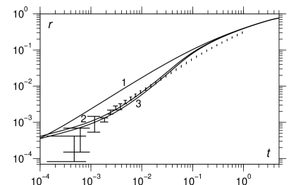
Figure 13: Bridge radius as a function of time for viscosity $\mu=48$ mPa s ($Re=68$) obtained using different models compared to experiments from (paulsen11, ) (with error bars). Curve 1: the conventional model; curve 2: the interface formation model with $\rho^{s}_{1e}=0.45$ and other parameters from (28); curve 3: the interface formation model with parameters from (28).

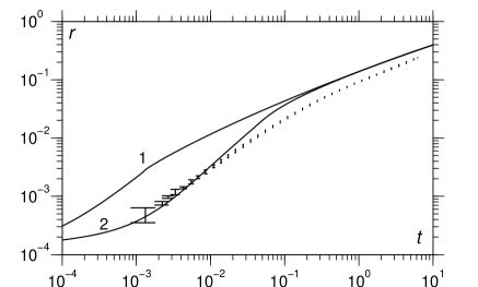
Figure 14: Bridge radius as a function of time for viscosity $\mu=48$ mPa s ($Re=1.4\times 10^{4}$) obtained using different models compared to experiments from (paulsen11, ) (with error bars). Curve 1: the conventional model and curve 2: the interface formation model with parameters from (28).

VIII Theory-guided experiments

VIII.1 Free-surface shape

Having found from the interface formation model that the free-surface shape is non-smooth for a considerable amount of time, it is reasonable to ask why this has not been reported from experiments and how this effect can be brought to light. Taking the largest viscosity used in these experiments ($230$ mPa s), we see from Figure 10 that the contact angle varies over the time period $10^{-2}<t<10^{-1}$ during which, from Figure 11, the bridge radius varies in the range $10^{-2}<r<10^{-1}$. In other words, whilst the bridge evolves from around $1$% to $10$% of the drop’s total radius, the free-surface profile is non-smooth. As can be seen in Figure 11, some data points from the experiments of (thoroddsen05, ) exist in this regime, so that, in principle, this regime is within the range of optical experiments. In fact, in (thoroddsen05, ), it is noted (see their Figure 20) that, as the viscosity increases, for a given bridge radius ($280$ $\mu$m) the curvature of the bridge’s profile increases rapidly as a function of viscosity. This is based on fitting circles to the free surface images to extract a radius of curvature, a process which (a) presumes that the free surface is smooth and (b) involves, as the authors admit, “some subjectivity”. In fact, our results obtained in the framework of the interface formation model suggest that, for the highest viscosity which we consider, when $r_{dim}=2.8\times 10^{-4}$ m, so that $r\approx 10^{-1}$, the free surface will indeed be almost smooth. However, if instead one considers $t=r=0.04$, which corresponds to a dimensional bridge radius of $80$ $\mu$m, then our results suggest that the contact angle should be measurable, at around $115^{\circ}$. This is apparently within the optical range. Furthermore, if one goes to higher viscosities, there is the possibility of making the contact angle even more pronounced.

It is interesting to note from Figure 10 that, when the angle is already not too large, i.e. $\theta_{d}<120^{\circ}$, the profiles obtained using the interface formation model (lower curves) do not look very sharp where they meet $z=0$, and one can easily see how, without allowing for the possibility that the free surface can be non-smooth, these angles could easily be attributed to the errors associated with the optical resolution.

Here, we are interested in suggesting theory-guided experiments, which would allow experimentally obtained data to be interpreted in terms of the concepts that the interface formation model adds to our conventional understanding of fluid mechanical phenomena, such as, in this particular case, describing how non-smooth free surface profiles can be sustained. With the aforementioned estimates in mind, we return to the highest viscosity fluid ($58000$ mPa s) used in (paulsen12, ), and consider whether one can bring the differences between the conventional model and the interface formation model into the optical range for these parameters. In Figure 15, we give an example showing that this is indeed possible. In particular, we see that with the time of the order of $100$ ms and the bridge radius of the order of $100$ $\mu$m, so that we are well within the optical range, there is a clearly verifiable difference between the two models’ predictions. It should be pointed out that we have not been able to ascertain the precise parameters which should be used for the interface formation model for this particular fluid, and so have used the parameters (28) mentioned earlier. The key point is that this is a perfect test case with which the use of the interface formation model for the coalescence process could be scrutinized.

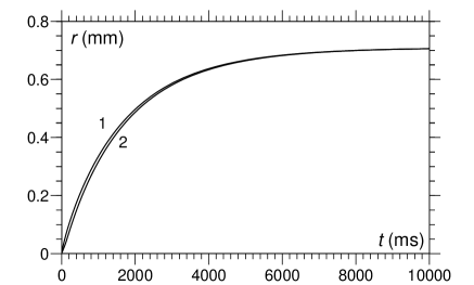
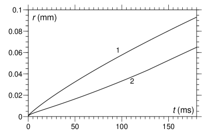
Figure 15: Example illustrating the dependence of the dimensional radius of the bridge on dimensional time for the coalescence of two liquid spheres of radius $1$ mm, viscosity $58000$ mPa s and surface tension $20$ mN m^-1 simulated using the conventional model (curve 1) and the interface formation model (curve 2). Although on a large time scale the two curves are similar, on a shorter, and yet easily measurable, time scale there are experimentally verifiable differences between the predictions of the two models.

VIII.2 Kinematics

Another aspect of the interface formation model that lends itself to experimental verification is the fact that the flow kinematics produced in the framework of this model indicates that the fluid particles initially belonging to the free surface move across the contact line to become the fluid particles forming, first, the internal interface and then the ‘ordinary’ bulk particles. In other words, there is a qualitative difference with what one has in the conventional model where the fluid particles once forming the free surface stay on the free surface at all time. From an experimental viewpoint, this difference suggests ‘marking’ the fluid particles of the free surface with microscopic ‘markers’, e.g. the molecules of a surfactant with a sufficiently low concentration so that the surfactant remains a ‘marker’, as opposed to influencing the fluid’s dynamics. Then, one could monitor the percentage of the ‘markers’ that find themselves in the bulk of the fluid when the drops coalesce to form a single body of fluid.

Notably, the kind of kinematics outlined above has been observed in the experiments on the steady free-surface ‘cusps’ forming in convergent flow(jeong92, ), albeit the ‘markers’ used in these experiments (particles of a powder) were rather crude. It is also worth mentioning that, as it has subsequently been shown, the ‘cusps’ themselves, first discovered in (joseph91, ), turned out to be corners(shik05a, ), so that the ‘contact angle’ in the coalescence phenomenon is actually the unsteady version of the corners observed in steady convergent flows. The similarity between the flow kinematics in the steady convergent flows and the coalescence process indicates that the appearance of singularities in the free-surface curvature and the corresponding qualitative change in the flow kinematics could be a generic phenomenon with profound implications.

IX Concluding remarks

Much literature on the coalescence of liquid drops has been concerned with producing and testing various ‘scaling laws’, which, with the proper choice of constants, are expected to approximate the actual solution one would obtain in the framework of the conventional model. Here, we have used our computational platform to show that in many cases these scaling laws indeed provide a fairly good fit to the predictions of the conventional model and in some cases appear to work even outside their ‘nominal’ limits of applicability. However, we have also shown that the conventional model itself is unable to describe the coalescence phenomenon whose details have come to light with the new experimental data. In fact, for the three viscosities considered, even on a $\log$-$\log$ plot there is a clear discrepancy between the predictions of the conventional model and experimental data in all cases except the late stages of coalescence of the most viscous drop, i.e. the stages where coalescence as such is already over. Clearly then, the scaling laws so often used in the literature are also ineffective at describing these flows and any attempts to fit the data with different coefficients will merely result in the dependencies that are no longer close to the solution of the equations they are supposed to represent.

The mathematical complexity of the interface formation model has often been cited (attane07, ; bayer06, ) as its drawback, although there is no reason to expect that intricate experimental effects will be describable by simple mathematics. We have overcome the mathematical difficulties of incorporating the interface formation model into a numerical platform in our previous work (sprittles_jcp, ), which allowed us to use and compare both the conventional and the interface formation model in the context of dynamic wetting processes. In the present work, we have shown that the interface formation model provides a natural description, as well as a considerably easier numerical implementation compared to the conventional model, for the coalescence phenomena. The reason for this is that the interface formation model is able to cope with the coalescence event in a singularity-free manner, which makes computation far easier and actually means that less resolution is required with this model than the conventional one. The results of using the interface formation model agree well with all experimental data apart from the late stages of low viscosity drops, in which coalescence as such, i.e. the formation of a single body of fluid with a smooth free surface, has actually occurred already.

As previously mentioned, it seems most likely that the influence of the surrounding air, which is neglected in our description, is responsible for the above discrepancy between the theories and experiment. The evidence in favour of this reason is that at the highest viscosity, where the liquid-to-air viscosity ratio is large, $\mu/\mu_{air}\sim 10^{4}$, there is no discrepancy whereas at the lowest liquid-to-air viscosity ratio $\mu/\mu_{air}\sim 10^{2}$, i.e. where the viscosities are more comparable, an influence is seen. Including the ambient gas dynamics will be the subject of future work where we will consider both the possibility of using lubrication theory to determine the forces acting on the free surface from the gas, as well as extending our computational framework to describe the gas flow.

Our computations have confirmed previous predictions that for low-viscosity fluids, toroidal bubbles are to be expected. Such bubbles are particularly prevalent when one uses the conventional model to describe coalescence as it introduces a stronger capillary wave that leads to the trapping of the bubbles. Therefore, a potential test case for the two models would be to predict when such bubbles exist and what the size distribution of the bubbles will be. The problem of describing the dynamics of the trapped bubbles and, in particular, their stability with respect to azimuthal disturbances, requires the development of more powerful computer codes which would be capable of handling multiple topological changes to the fluid’s domain. This is the subject of current work. From the theoretical standpoint, it is yet unclear even how accounting for the ambient gas’ viscosity will affect the formation of the bubbles, and a natural approach to this problem is to include the gas dynamics into the computational framework. Ultimately, it will be for the experiments to ascertain the appearance of the toroidal bubbles and the conditions that promote this effect. In this regard, experiments in vacuum/low-pressure chambers are a particularly promising line of enquiry as they could help to elucidate several aspects associated with the role of the gas.

Much debate exists in the literature as to whether the conventional model and its known extensions are able to describe a variety of flow configurations in which, as suggested by qualitative analysis, interfaces form or disappear. These flows are often characterized by the conventional model predicting singularities of various kind, as is the case for coalescence (shik00, ), or not allowing a solution to exist at all, as in the case of dynamic wetting (shik07, ). The advantage of using the coalescence phenomena to investigate the possibility of dynamic interfacial effects is that, in contrast to dynamic wetting experiments, there is no solid surface involved; the solid’s properties, such as roughness and chemical inhomogeneity, are usually poorly defined, which creates room for different interpretations of the experimental outcome. If viewed through the prism of the interface formation model, the coalescence process considered here can be regarded essentially as the ‘dynamic wetting’ of a geometric surface (plane of symmetry), where the ‘equilibrium contact angle’ is $90^{\circ}$. In other words, in coalescence, any observed non-smoothness of the free surface is evidence in favour of the interface formation model. Furthermore, the known effect of ‘hydrodynamic assist of dynamic wetting’ (blake99, ; blake94, ) suggests that in the coalescence process, for the same liquid, the dynamic contact angle versus contact-line speed curves will depend on the drops’ size, and a close investigation of this effect could provide valuable information about the interfacial dynamics.

Our results suggest that, as drops’ size decreases, the deviation between the conventional and the interface formation model will become more pronounced as the relative size of the trapped ‘internal interface’ will increase, which is particularly the case for high-viscosity liquids. However, as the size of the system goes down, one runs into the limitations of what can be measured using the conventional optical techniques. To a certain extent, this catch twenty-two situation has been resolved by the pioneering experiments from the Chicago Group, e.g. (paulsen11, ), which allow, for the first time, sub-optical measurements to be made reliably and accurately. It would be interesting to see if a similar method can be applied to wetting experiments to allow a similar resolution to be achieved there, i.e. to determine the radius of the wetted area for a drop impact and spreading onto a solid substrate as a function of time from the resistance which this area produces. Such a method could uncover the new effects predicted in (sprittles_jcp, ), which are similar to those observed in coalescence, namely that, as the interface formation model indicates, the onset of spreading corresponds to a much slower initial motion of the wetting line than what the conventional models suggest. Of particular importance is the predicted decrease of the dynamic contact angle as the contact-line speed increases, which is a specific feature of unsteady dynamic wetting.

It was interesting to see that, with regard to the coalescence experiments, a better agreement between theory and experiment was obtained by using a lower value of $\rho^{s}_{1e}$ as the concentration of glycerol was increased in the mixture. As both water and glycerol have a similar density, this may seem somewhat surprising; however, the hygroscopic nature of glycerol suggests that at high concentrations often the interface of the drops can consist of just one of the liquids, which then essentially acts as a kind of surfactant to the whole mixture. We can speculate that this may be the nature of the observed effect, but the best way to confirm that this is the case would be to use a different liquid, such as a silicon oil, which does not suffer from such effects, in order to conduct similar experiments and then, by checking the results against the interface formation model’s simulations, determine whether there is a variation of $\rho^{s}_{1e}$ with, say, viscosity.

Appendix: Influence of initial gravity and initial shape

To simulate the coalescence of two drops, which retain their axisymmetry but, due to, say, gravity, lose their symmetry about the $z=0$ plane is a computationally tractable problem. Here we have assumed that such asymmetry will not have a significant influence on the very initial stages of coalescence and, in particular, will not alter the conclusions of our comparison between theory and experiment. Once gravity is included, it will act to elongate/squash the upper/lower drop so that the radius of curvature of the upper/lower drop at the point where the two drops meet is decreased/increased. Then, crudely, one could argue that these two opposite influences, which will act to decrease/increase the speed of coalescence, will neutralize each other. To provide bounds on the effects which gravity could have, whilst retaining the plane of symmetry, we consider a body force which acts towards the $z=0$ plane, so that the drop, and its image, is elongated and the opposite case where the body force is away from the $z=0$ plane, acting to squash the drop. These tests, which provide the worst case scenario where a elongated/squashed drop coalesces with a copy of itself, so that there is no cancelling of effects, will provide a useful bounds on the influence that correctly incorporating gravity into our framework would have.

In Figure 16, we see the influence which gravity has on the initial shapes and the subsequent evolution of the drops considered in (paulsen11, ), which are taken for the $Re=68$ case. The bridge radius is plotted for simulations using the conventional model with the two elongated drops (curve 1) and the two squashed drops (curve 2) compared to the zero gravity case (dashed curve), where perfect hemispheres coalesce. Also in the figure are the experimental error bars from (paulsen11, ) and, most importantly, one can see that over the range $0<t<1$, the effect of the initial shape, has very little influence on the drops’ dynamics.

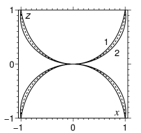
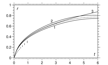
Figure 16: Left: Different initial shapes dependent on gravity for $2$ mm drops. Right: Bridge radius as a function of time for the drops with $Re=68$ compared to error bars from (paulsen11, ), with curve 1 corresponding to $Bo=0.74$, curve 2 to $Bo=-0.74$ and the dashed curve is the hemispheres obtained for $Bo=0$. Curve 3 is for the coalescence of free spheres as opposed to pinned hemispheres.

Additionally, in Figure 16, we show that the non-local effect of the different flow geometries used, i.e. free spheres and pinned hemispheres, have no influence on the very initial stages of coalescence, where the comparison to experiment has been made. As one can see, in this region the result for coalescing hemispheres (dashed line) is graphically indistinguishable from that obtained using spheres (curve 3). Notably, the two equilibrium bridge radii will differ, with the sphere obtaining a larger equilibrium radius.

References

- (1) C. T. Bellehumeur, M. K. Biaria, and J. Vlachopoulos, “An experimental study and model assessment of polymer sintering,” Polymer Engineering and Science 36, 2198–2207 (2004)
- (2) T. M. Dreher, J. Glass, A. J. O’Connor, and G. W. Stevens, “Effect of rheology on coalescence rates and emulsion stability,” AIChE Journal 45, 1182–1190 (1999)
- (3) W. M. Grissom and F. A. Wierum, “Liquid spray cooling of a heated surface,” International Journal of Heat and Mass Transfer 24, 261–271 (1981)
- (4) A. Kovetz and B. Olund, “The effect of coalescence and condensation on rain formation in a cloud of finite vertical extent,” Journal of Atmospheric Sciences 26, 1060–1065 (1969)
- (5) T. M. Squires and S. R. Quake, “Microfluidics: Fluid physics at the nanoliter scale,” Reviews of Modern Physics 77, 977–1026 (2005)
- (6) B. Derby, “Inkjet printing of functional and structural materials: Fluid property requirements, feature stability and resolution,” Annual Review of Materials Research 40, 395–414 (2010)
- (7) M. Singh, H. Haverinen, P. Dhagat, and G. Jabbour, “Inkjet printing process and its applications,” Advanced Materials 22, 673–685 (2010)
- (8) S. Richardson, “Two-dimensional bubbles in slow viscous flows,” Journal of Fluid Mechanics 33, 475–493 (1968)
- (9) S. T. Thoroddsen, K. Takehara, and T. G. Etoh, “The coalescence speed of a pendent and sessile drop,” Journal of Fluid Mechanics 527, 85–114 (2005)
- (10) J. D. Paulsen, J. C. Burton, and S. R. Nagel, “Viscous to inertial crossover in liquid drop coalescence,” Physical Review Letters 106, 114501 (2011)
- (11) J. Frenkel, “Viscous flow of crystalline bodies under the action of surface tension,” Journal of Physics (USSR) 9, 385–391 (1945)
- (12) R. W. Hopper, “Coalescence of two equal cylinders: exact results for creeping viscous plane flow driven by capillarity,” Journal of the American Ceramic Society 67, 262–264 (1984)
- (13) R. W. Hopper, “Plane Stokes flow driven by capillarity on a free surface,” Journal of Fluid Mechanics 213, 349–375 (1990)
- (14) R. W. Hopper, “Coalescence of two viscous cylinders by capillarity: Part 1. Theory,” Journal of the American Ceramic Society 76, 2947–2952 (1993)
- (15) R. W. Hopper, “Coalescence of two viscous cylinders by capillarity: Part 2. shape evolution,” Journal of the American Ceramic Society 76, 2953–2960 (1993)
- (16) S. Richardson, “Two-dimensional slow viscous flows with time-dependent free boundaries driven by surface tension,” European Journal of Applied Mathematics 3, 193–207 (1992)
- (17) J. Eggers, J. R. Lister, and H. A. Stone, “Coalescence of liquid drops,” Journal of Fluid Mechanics 401, 293–310 (1999)
- (18) L. Duchemin, J. Eggers, and C. Josserand, “Inviscid coalescence of drops,” Journal of Fluid Mechanics 487, 167–178 (2003)
- (19) A. Menchaca-Rocha, A. Martínez-Dávalos, R. Núńez, S. Popinet, and S. Zaleski, “Coalescence of liquid drops by surface tension,” Physical Review E 63, 046309 (2001)
- (20) J. D. Paulsen, J. C. Burton, S. R. Nagel, S. Appathurai, M. T. Harris, and O. Basaran, “The inexorable resistance of inertia determines the initial regime of drop coalescence,” Proceedings of the National Academy of Science 109, 6857–6861 (2012)
- (21) H. N. Oguz and A. Prosperetti, “Surface-tension effects in the contact of liquid surfaces,” Journal of Fluid Mechanics 203, 149–171 (1989)
- (22) A. Jagota and P. R. Dawson, “Micromechanical modeling of powder compacts - I. Unit problems for sintering and traction induced deformation,” Acta Metallurgica 36, 2551–2561 (1988)
- (23) J. I. Martínez-Herrera and J. J. Derby, “Viscous sintering of spherical particles via finite element analysis,” Journal of the American Ceramic Society 78, 645–649 (1995)
- (24) D. G. A. L. Aarts, H. N. W. Lekkerkerker, H. Guo, G. H. Wegdam, and D. Bonn, “Hydrodynamics of droplet coalescence,” Physical Review Letters 05, 164503 (2005)
- (25) M. Wu, T. Cubaud, and C. Ho, “Scaling law in liquid drop coalescence driven by surface tension,” Physics of Fluids 16, 51–54 (2004)
- (26) It should be pointed out here that the measurements are taken for relatively large bridge radii, so that a comparison with the inertial scaling (2) is valid, but the theory of duchemin03 is well past its limits of applicability, so that one cannot expect good agreement for the proposed prefactor.
- (27) S. C. Case and S. R. Nagel, “Coalescence in low-viscosity liquids,” Physical Review Letters 100, 084503 (2008)
- (28) S. C. Case, “Coalescence of low-viscosity fluids in air,” Physical Review E 79, 026307 (2009)
- (29) J. C. Burton, J. E. Rutledge, and P. Taborek, “Fluid pinch-off dynamics at nanometer length scales,” Physical Review Letters 92, 244505 (2004)
- (30) Y. D. Shikhmurzaev, “Coalescence and capillary breakup of liquid volumes,” Physics of Fluids 12, 2386–2396 (2000)
- (31) D. D. Joseph, J. Nelson, M. Renardy, and Y. Renardy, “Two-dimensional cusped interfaces,” Journal of Fluid Mechanics 223, 383–409 (1991)
- (32) Y. D. Shikhmurzaev, “Singularity of free-surface curvature in convergent flow: Cusp or corner?.” Physics Letters A 345–385, 378 (2005)
- (33) Y. D. Shikhmurzaev, “Capillary breakup of liquid threads: A singularity-free solution,” IMA Journal of Applied Mathematics 70, 880–907 (2005)
- (34) Y. D. Shikhmurzaev, “Macroscopic mechanism of rupture of free liquid films,” Comptes Rendus Mecanique 333, 205–210 (2005)
- (35) Y. D. Shikhmurzaev, “The moving contact line on a smooth solid surface,” International Journal of Multiphase Flow 19, 589–610 (1993)
- (36) Y. D. Shikhmurzaev, “Moving contact lines in liquid/liquid/solid systems,” Journal of Fluid Mechanics 334, 211–249 (1997)
- (37) Y. D. Shikhmurzaev, “Singularities at the moving contact line. Mathematical, physical and computational aspects,” Physica D 217, 121–133 (2006)
- (38) Y. D. Shikhmurzaev, “Spreading of drops on solid surfaces in a quasi-static regime,” Physics of Fluids 9, 266–275 (1996)
- (39) Y. D. Shikhmurzaev, Capillary Flows with Forming Interfaces (Chapman & Hall/CRC, Boca Raton, 2007)
- (40) J. E. Sprittles and Y. D. Shikhmurzaev, “Finite element simulation of dynamic wetting flows as an interface formation process,” Journal of Computational Physics 233, 34–65 (2013)
- (41) T. D. Blake and Y. D. Shikhmurzaev, “Dynamic wetting by liquids of different viscosity,” Journal of Colloid and Interface Science 253, 196–202 (2002)
- (42) T. Young, “An essay on the cohesion of fluids,” Philosophical Transactions of the Royal Society (London) 95, 65–87 (1805)
- (43) J. E. Sprittles and Y. D. Shikhmurzaev, “A finite element framework for describing dynamic wetting phenomena,” International Journal for Numerical Methods in Fluids 68, 1257–1298 (2012)
- (44) J. E. Sprittles and Y. D. Shikhmurzaev, “The dynamics of liquid drops and their interaction with solids of varying wettabilities,” Physics of Fluids 24, 082001 (2012)
- (45) S. F. Kistler and L. E. Scriven, “Coating flows,” in Computational Analysis of Polymer Processing, edited by J. R. A. Pearson and S. M. Richardson (Applied Science Publishers London and New York, 1983) pp. 243–299
- (46) M. Heil, “An efficient solver for the fully-coupled solution of large displacement fluid-structure interaction problems,” Computer Methods in Applied Mechanics and Engineering 193, 1–23 (2004)
- (47) M. C. T. Wilson, J. L. Summers, Y. D. Shikhmurzaev, A. Clarke, and T. D. Blake, “Nonlocal hydrodynamic influence on the dynamic contact angle: Slip models versus experiment,” Physical Review E 83, 041606 (2006)
- (48) P. Lötstedt and L. Petzold, “Numerical solution of nonlinear differential equations with an algebraic constraints 1: Convergence results for backward differentiation formulas,” Mathematics of Computation 46, 491–516 (1986)
- (49) P. M. Gresho and R. L. Sani, Incompressible Flow and the Finite Element Method. Volume 2. Isothermal Laminar Flow (John Wiley & Sons, LTD, New York, 1999)
- (50) O. A. Basaran, “Nonlinear oscillations of viscous liquid drops,” Journal of Fluid Mechanics 241, 169–198 (1992)
- (51) We can see this from the data provided to us by Dr J.D. Paulsen, Dr J.C. Burton and Professor S.R. Nagel, which was published in paulsen11 .
- (52) Despite the drops in thoroddsen05 having a different radius, mm, and very slightly different viscosity, mPa s, our simulations show that at such high viscosity these alterations can be scaled out by an appropriate choice of viscous time-scale, as we use.
- (53) S. Fordham, “On the calculation of surface tension from measurements of pendant drops,” Proceedings of the Royal Society of London. Series A: Mathematical and Physical 194, 1–16 (1948)
- (54) More precisely, it is the conventional model as at this stage the interface formation/disappearance dynamics have ended, so that the interfaces are in equilibrium and the interface formation model becomes equivalent to the conventional one.
- (55) J. -T. Jeong and H. K. Moffatt, “Free-surface cusps associated with flow at low Reynolds number,” Journal of Fluid Mechanics 241, 1–22 (1992)
- (56) P. Attané, F. Girard, and V. Morin, “An energy balance approach of the dynamics of drop impact on a solid surface,” Physics of Fluids 19, 012101 (2007)
- (57) I. S. Bayer and C. M. Megaridis, “Contact angle dynamics in droplets impacting on flat surfaces with different wetting characteristics,” Journal of Fluid Mechanics 558, 415–449 (2006)
- (58) T. D. Blake, M. Bracke, and Y. D. Shikhmurzaev, “Experimental evidence of nonlocal hydrodynamic influence on the dynamic contact angle,” Physics of Fluids 11, 1995–2007 (1999)
- (59) T. D. Blake, A. Clarke, and K. J. Ruschak, “Hydrodynamic assist of wetting,” AIChE Journal 40, 229–242 (1994)