Direct Evidence for a Fast CME Driven by the Prior Formation and Subsequent Destabilization of a Magnetic Flux Rope

Abstract

Magnetic flux ropes play a central role in the physics of Coronal Mass Ejections (CMEs). Although a flux rope topology is inferred for the majority of coronagraphic observations of CMEs, a heated debate rages on whether the flux ropes pre-exist or whether they are formed on-the-fly during the eruption. Here, we present a detailed analysis of Extreme Ultraviolet observations of the formation of a flux rope during a confined flare followed about seven hours later by the ejection of the flux rope and an eruptive flare. The two flares occured during 18 and 19 July 2012. The second event unleashed a fast ($>$ 1000 $\mathrm{km\,{s}^{-1}}$) CME. We present the first direct evidence of a fast CME driven by the prior formation and destabilization of a coronal magnetic flux rope formed during the confined flare on 18 July.

1 Introduction

All currently available theories of CME formation predict that CMEs are basically ejections of magnetic flux ropes. This prediction is largely confirmed by coronagraphic observations of CMEs in the outer corona showing that the majority exhibits a clear flux rope geometry (at least $\sim$ 40% Vourlidas et al., 2012a). However, an intense debate exists on whether such a magnetic topology exists before the CME onset or whether it is formed during the CME eruption (see for example the reviews of Forbes, 2000; Klimchuk, 2001; Chen, 2011). A conclusive answer to this question would represent an important advance in our understanding of CMEs. There are models of CME initiation which form the flux rope once the CME is underway, i.e. on-the-fly, while others require a pre-existing flux rope before the CME onset. A further division in the latter models concerns the origin of the flux rope. It may be formed either in the corona, coronal flux rope (e.g, Moore & Roumeliotis, 1992; Antiochos et al., 1999; Amari et al., 2000; Lynch et al., 2008; Vršnak, 2008), or in the photosphere or low chromosphere, photospheric flux rope (e.g., Magara & Longcope, 2001; Manchester et al., 2004; Gibson & Fan, 2006; Archontis & Hood, 2008) after the emergence of a twisted flux tube from the convection zone.

Significant progress into this problem has been achieved for CMEs originating from quiet Sun (QS) regions, such as those associated with Polar Crown Filaments. Observations in various spectral domains like the White Light (WL) the extreme ultraviolet (EUV) and soft Xrays (SXRs), has shown large-scale quiescent cavities going through a quasi-static rise phase, with a duration of up to several days, which could eventually erupt giving rise to CMEs (e.g., Engvold, 1989; Hudson et al., 1999; Koutchmy et al., 2004; Gibson et al., 2006; Su et al., 2010; Régnier et al., 2011). Cavity densities are typically lower and their temperatures are higher than the background corona values (e.g., Fuller et al., 2008; Vásquez et al., 2010; Kucera et al., 2012; Reeves et al., 2012). It is widely acknowledged today that the observed cavities (or at least part of their cross section) correspond to a magnetic flux rope seen edge-on. Further evidence for a flux rope topology in QS cavities comes from polarization signals of the coronal magnetic field (Dove et al., 2011), from swirling motions observed in these structures (Wang & Stenborg, 2010) and from concave-upward structures in CME cavities (Plunkett et al., 2000; Robbrecht et al., 2009; Vourlidas et al., 2012a). Therefore, the pre-existing flux rope scenario seems very viable for CMEs originating in the QS. Finally, prominences either quiescent or eruptive often exhibit helical structures, which represents a strong indication of a flux rope topology (e.g., Vrsnak et al., 1991; Romano et al., 2003; Rust & LaBonte, 2005; Williams et al., 2005; Chen et al., 2006). Note that is widely believed today that helical prominences correspond to only the lower parts of flux ropes, where dense material is collecting.

However, the situation is unclear for impulsive CMEs originating in active regions (ARs). This is due to several physical and geometrical factors. First, the prevalence of higher magnetic field orders in ARs compared to QS implies that the CME-related structures (cavity, flux rope, etc) will be both smaller in size and lower-lying in ARs compared to the QS. This would make it difficult to identify any pre-existing flux rope, especially when we consider the line-of-sight (LOS) interfence from the EUV emission of the myriads of loops lying at more or less random orientations in the low corona. Second, impulsive CMEs in ARs evolve at relatively short time-scales because of the smaller spatial scales and higher Alfvén speeds in ARs compared to the QS (e.g. Vršnak et al., 2007). The rapid evolution would make it extremely difficult to discriminate between pre-existing and on-the-fly formed flux ropes. Indeed, recent high cadence observations of impulsive CME onsets have placed strong constraints on the initial sizes and timescales of potential flux ropes (e.g. Patsourakos et al., 2010a; Patsourakos et al., 2010b; Vourlidas et al., 2012b). These limits were inferred from observations of the formation and evolution of CME cavities in the EUV, and showed that CME flux ropes could be initially very small (radius $<$ 0.01 $\mathrm{R_{\odot}}$) and low-lying (height $<$ 0.1 $\mathrm{R_{\odot}}$) and could evolve in short time scales of the order of 1-2 minutes. Third, impulsive CMEs from ARs are always associated with significant plasma heating in the form of a flare. According to the standard CME-flare CSHKP model (e.g., Carmichael, 1964; Sturrock, 1966; Hirayama, 1974; Kopp & Pneuman, 1976), one part of the reconnected magnetic flux under the erupting CMEs is directed towards the flare loops and the other part is added to the erupting flux rope. Hence, the erupting flux ropes will be (at least initially) substantially heated. Therefore, CME flux ropes should appear in hot, flare-like, EUV wavelengths which were not routinely observed at high cadence until recently. Taken together, these four reasons explain why flux ropes, whether pre-existing or not, are so elusive in impulsive CMEs.

Non-linear force free magnetic field extrapolations and flux rope insertion methods reveal magnetic field distributions pertinent to flux ropes in ARs which could eventually erupt (e.g., Canou et al., 2009; Savcheva & van Ballegooijen, 2009). Although quite valuable, such calculations rely upon the observed photospheric magnetic field which does not change significantly over large areas during eruptions. Therefore, such methods may not be particularly helpful for tracking the (presumably) rapidly changing coronal magnetic fields during CMEs. This limitation together with the frozen-in property of coronal plasmas to the coronal magnetic field make rapid, narrow-band multi-thermal EUV imaging going all the way from flare down to transition region temperatures a very powerful tool to study rapid changes in the coronal field during CME onsets.

Strong, but indirect, evidence for pre-existing flux ropes comes from EUV and SXR observations of the formation and eventual eruption of sigmoids (e.g., Aurass et al., 1999; Canfield et al., 1999; Vrsnak, 2003; Green & Kliem, 2009; Tripathi et al., 2009; Liu et al., 2010; Green et al., 2011; Huang et al., 2011). EUV and SXR sigmoids are interpreted as disk signatures of flux ropes viewed from above. Since sigmoids are optimally observed from above, projection effects may enter into the interpretation of the observations (e.g. structures at different heights may appear connected in projection). SXR observations of an eruptive flare by SXT showed the formation of an oval-shaped structure, highly suggestive of a flux rope core, at the onset of the impulsive CME acceleration and simultaneously with the appearance of the X-ray flare loops (Vršnak et al., 2004). Moreover, SXT and XRT observations showed evidence of cusp-shaped loops forming under the erupting flux which sometimes has a concave upwards V-shape (e.g., Tsuneta et al., 1992; Tsuneta, 1997; Savage et al., 2010). All these features are predicted by the standard solar eruption model. More recently, EUV observations in flare temperatures ($\approx$ 10 MK) of CME onsets at or close to the solar limb showed the formation of a magnetic flux rope a few minutes before the onsets of the associated CMEs and flares (Cheng et al., 2011; Zhang et al., 2012), with its upper part resembling a plasmoid structure (Reeves & Golub, 2011).

Finally, the question of whether the flux rope forms before or during the eruption has broad implications for the CME initiation mechanism(s). The answer will determine whether the eruption process is ideal (prior flux rope) or resistive (on-the-fly flux rope). As we argued, the question was very difficult, if not impossible, to answer until recently because of low cadence and sensitivity, and lack of observations in appropriate hot EUV lines. The availability of high cadence, multi-wavelenth EUV observations from the Atmospheric Imaging Assembly (AIA; Lemen et al., 2012) aboard the Solar Dynamics Observatory (SDO) since 2010 and the multiviewpoint observations from the EUV Imager (EUVI; Wuelser et al., 2004) in the Sun Earth Connection Coronal and Heliospheric Investigation (SECCHI; Howard et al., 2008) imaging suite aboard the STEREO mission have greatly improved the situation.

In this paper,we directly address the question of the pre-existing fluxrope for a fast ($>$ 1000 $\mathrm{km\,{s}^{-1}}$) CME that erupted on 2012 July 19. We take advantage of detailed EUV observations, spanning several hours, of its source region before the eruption. The multi-temperature coverage from the AIA images allows us to detect and follow (thermally and kinematically) the formation and evolution of a very clear flux rope structure on July 18 at $\approx$ 22:20 UT during a confined flare. The EUVI observations allow us to reconstruct its three-dimensional (3D) morphology. The flux rope finally erupts on July 19 at around 05:20 UT creating the fast CME. We present the EUV observations and analysis of the flux rope in Section 2 and the inferred 3D structure in Section 3. In Section 4, we discuss the evolution of the flux rope and the implications for CME intiation theories. We conclude in Section 5.

2 Observations and Data Analysis

We analyzed EUV images of the low corona (1-1.3 $\mathrm{R_{\odot}}$and 1-1.6 $\mathrm{R_{\odot}}$, respectively) from the SDO/AIA and STEREO/EUVI, and WL images of the outer corona (2.2-6 $\mathrm{R_{\odot}}$) from the Large Angle and Spectrometric Coronograph (LASCO; Brueckner et al., 1995) C2 coronagraph on board the SOHO mission.

We used AIA images (level 1.5) recorded in narrow-band channels centered at $\approx$ 304, 171, 193, 211, 335, 94 and 131 Å, which have peak responses at temperatures of $\approx$ 0.05, 0.6, 1.6, 2.0, 2.5, 6.3 and 10 MK respectively; EUVI images from the 195 Å  channel having a peak response for $\approx$ 1.6 MK were also used. In the rest of the paper we will refer to any given channel by simply supplying the wavelength of peak response: for example 304 Å  channel will be referred to as 304. The signal in 94 and 131 is dominated by multi-million plasmas only when intense heating, usually associated with flares, takes place. As we will see, the AIA capability to obtain narrow-band images of ultra-hot plasmas is a decisive factor in understanding the eruption process in this event. Under quiescent conditions the signal in 94 and 131 is dominated by cool emissions formed below 1 MK. Moreover, total brightness images of the corona taken by LASCO on SOHO were analyzed. To reduce data volume, we used AIA images with a reduced cadence of 1 minute. Inspection of full cadence movies during the $\sim 9$ hour window of our investigation showed that the one minute cadence was sufficient to resolve the various dynamics. The cadence of the STA 195 and LASCO images was 5 and 12 minutes, respectively. Pixel sizes for AIA, EUVI and LASCO C2 images are 0.6, 1.6 and 12 arcsec respectively. To enhance the image contrast in the corresponding EUV images we have processed the original data with wavelets (Stenborg et al., 2008) to bring out their fine structure; we essentially subtracted from each frame a “background” frame resulting from a wavelet-filtered version of the frame amplifying only the low spatial frequencies (i.e., enhancing tha large-scale structure). However, every flux measurement was carried out on the original data.

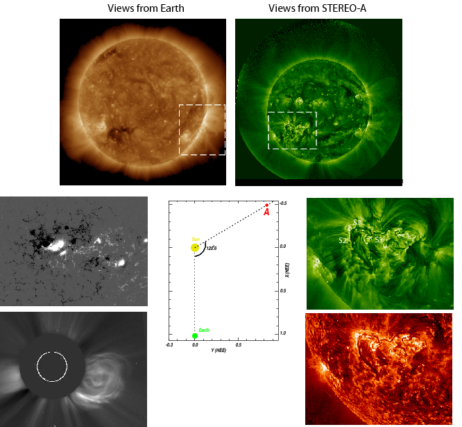
Figure 1: Context information for the flare and CME events in this study. Middle panel: Relative positions of Earth, Sun and STA during our observations. Left panels: Earth-based views of the source AR. (top) AIA 193 image on 2012 July 18. (Middle) HMI magnetogram on 2012 July 12, close to the central meridian passage of the AR as seen from the Earth. (Bottom) LASCO C2 image showing the CME associated with the eruptive flare on July 19. Right panels: Views from STA on 2012 July 18. (top) 195 full disk image. (Middle) detail of the source AR in 195 and 304 (bottom). The boxes in the upper panels contain the source AR.

Our target was NOAA active region (AR) 11520. This AR was particularly active and hosted several flares and CMEs. We hereby focus on the time interval from $\approx$ 21 UT on 2012 July 18 until 06 UT on July 19 when AR11520 hosted a confined C4.5 flare (peaked at $\sim 22$ UT on July 18) and an eruptive M7.7 flare (peaked at $\sim$ 06 UT on July 19). The eruptive flare was associated with a WL CME observed later on by LASCO C2. Figure 1 summarizes the events as seen from different perspectives. During the period of interest, 11520 was located at the West limb as seen from AIA (Earth) and at almost $30^{\circ}$ East off the central meridian as viewed from EUVI on STEREO Spacecraft A (EUVI-A, hereafter), which was $120.6^{\circ}$ ahead of the Earth. Thus we had both edge-on (AIA) and face-on (EUVI-A) observations of the target AR. Figure 1 also shows the photospheric magnetic field distibution around AR11520 on July 12, when the AR crossed the central meridian passage as viewed from Earth using the Helioseismic and Magnetic Imager (HMI; Scherrer et al. (2012)) on SDO. The complexity of the photospheric magnetic field is obvious. A curved neutral line (NL) shape can be inferred from the magnetic field distribution. Proxies of the NL shape and extensions during the period of interest could be inferred by the inspection of dark filament material images of the target AR as seen from above in 304 and 195 EUVI-A images. The NL was quite long and complex and consisted of several approximately linear segments forming a mirrored “?” shape starting from the eastern end of S3, continuing along S1 and S2 and extending farther southward. The AIA LOS was aligned with horizontal element S1, vertical element S2 was running north-to-south parallel to the West limb as seen from the Earth, and element S3 was well behind the West limb and therefore was invisible from Earth. Note the sheared shape of the NL at the junction connecting S1 and S2. This was probably related to a rotating spot dragging and shearing the magnetic field at this location. This feature may have significant implications for the AR evolution. The footpoint alignment between the AIA LOS and element S1 was an important factor for observing the flux rope structure, as we will see later.

In the following subsections we organize our observations into three distinct phases. Their synthesis into a cohesive physical and geometrical scenario comes in Sections 3 and 4.

2.1 Formation of the Flux Rope and Failed Eruption

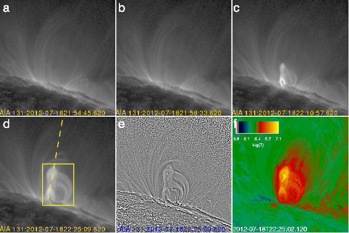
Figure 2: Representative snapshots in the 131 channel of the confined flare. (a) The pre-event configuration, (b) the start of the flux rope rise, (c) the full development of the flux rope and (d) the ‘flux rope reaches a stable height and size. The images are scaled logarithmically. Panel (e) shows a wavelet-enhanced version of panel (d) to highlight fine structure within the flux rope. (f) Temperature map at the time of panel (d). The field of view is 600$\times$ 600 $\mathrm{{arcsec}^{2}}$. The images have been rotated so that East-West represents the vertical direction. The box and the dashed line overplotted on panel (d) depict an area and path used in the construction of Figures 6 and 8, respectively.

The first phase consists of a confined flare on July 18 accompanied by the formation of a very clear flux rope structure. These events are readily observed in the 131 online movie (movie1.mp4). Figure 2 contains several snapshots from this movie. Starting at around 22:00 UT, we observe the rise of a narrow structure above the western limb (Figure 2b). Eventually, the structure exhibits a core, with an elliptical cross-section, and several ’legs’ threading the core and connecting only on the southern side (Figure 2c). In addition, cusp-like loops appeared underneath the core of the structure (Figure 2d). The structure bears a stricking resemblance to cartoon depictions and MHD model snapshots of magnetic flux ropes.

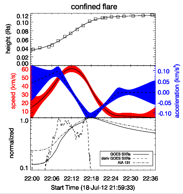
Figure 4: Confined flare. Top: temporal evolution of the flux rope height based on measurements in AIA 131 Å  (squares). The associated uncertainties are too small to be seen in this scale. The heights resulting from the application of a smoothing cubic spline to the original measurements are plotted with a solid black line. Middle: first (velocity) and second (acceleration) temporal derivatives of the smoothed height measurements (solid and dashed black lines respectively). Point-wise 1-$\sigma$ uncertainties in the velocity (red) and acceleration (blue) from 1000 Monte-Carlo simulations of the (assumed) Gaussian $h-t$ uncertainties. Bottom: normalized light curves of the GOES 1-8 Å  flux (solid line), its temporal derivative (dashed line) and the 131 light curve in the box encapsulating the flux rope structure in Figure 2d (dashed-dotted line).

Just 25 minutes after its start, the structure stops rising. Concurrently with these motions, a C4.5 flare from the same active region is taking place. The bright cusp-like loops are associated with the flare, as a quick inspection of the GOES SXI images reveals. No permanent dimmings are detected across the various AIA EUV channels over the area covered by the rising structure. No CME is seen in the LASCO C2 image, expect for an evanescent compression wave. These observations are consistent with the ’failed CME’ events identified in Vourlidas et al. (2010). The wave is very likely a compression wave launched by the ascent of the structure (piston-driven). Although it remains a possibility, it is unlikely that the wave could be launched by a flare-related pressure pulse because the flare heating occurs after the rise phase (Figure 4). As we will see in the next section, we find direct evidence of cooling of the flare plasmas entrained within the structure. Therefore, these observations suggest strongly that we are dealing with a failed eruption and consequently with a confined flare.

The most interesting and novel aspect of these observations is that the “core+legs” structure formed during the confined flare represents a clear example (possibly the clearest example in the literature so far) of a magnetic flux rope. We believe that this is the case for the following reasons:

1. It exhibits a coherently evolving large-scale structure enclosing intertwined threads (see for example the high-pass filtered image in Figure 2d). The coherency implies that the observed structure is a single macroscopic structure (an essential element for a magnetic flux rope interpretation) and not the fortuitous alignment, along the LOS, of the expansions of individual loops. Compare, for example, with the “independent” loop expansions observed prior to CME cavity formation (e.g., Patsourakos et al., 2010b; Patsourakos et al., 2010a). The internal fine coiling structure is a major ingredient of any magnetic flux rope.

2. It is formed by magnetic reconnection. The observations show that the 131 “core+legs” structure is appear concurrently with the cusp-shaped loops underneath, which also stretch and rise during the ascent of the structure. This is probably the most straightforward evidence that magnetic reconnection is forming a magnetic flux rope. According to the standard model of solar eruptions, the erupting flux generates coiled field lines which become part of a newly-formed (or add new flux to a pre-existing) flux rope. Interestingly, our observations show that the core is formed progressively through the continuous addition of new outer layers. This is the expectation from reconnection adding new flux to a flux rope (e.g., Lin et al., 2004). The cusp underneath the erupting flux represents the boundary between the most recently reconnected magnetic field lines which were either retracted downwards to form the post-eruption loops (i.e. the flare loops) or upwards to become part of the flux rope. A current sheet is expected to form between the tip of the cusp and the bottom of the flux rope. Finally, we note that the cusp and the narrow lower part of the flux rope core resemble an ”X”. This is strongly suggestive of the formation of a coronal X-point, in 2D, or more generally of a quasi-separatrix layer (QSL), in 3D (e.g., Aulanier et al., 2010; Savcheva et al., 2012). QSL layers separate domains of distinctively different magnetic topology, like flux rope and non flux rope fields in our case. Strong currents are expected to develop there. More importantly, QLSs represent regions where magnetic reconnection can occur easily.

3. It is very hot ($\sim 10$ MK) because it is initially visible only in the 131 channel. The temperature map in Figure 2f corraborates that the structure attains temperatures of around 10 MK during the confined flare. The map is calculated from a Differential Emission Measure (DEM) analysis of the AIA fluxes in the six EUV coronal channels (94, 131, 193, 171, 211, and 335) taken almost simultaneously during the confined flare. We use the methods and software described in Aschwanden et al. (2011). Essentially, a Gaussian DEM is simultaneously fitted to the observed fluxes in each pixel. Our fitting searches for DEM peak temperatures in the range 0.5-25 MK. The displayed temperature map in Figure 2f corresponds to temperature of the peak best-fit DEM. The flux rope reached a maximum temperature of $\approx$ 12 MK. Since the ”core+legs” 131 structure gets, at least initially, as hot as the flare loops underneath, their formation is likely sharing a common physical origin. This must be the reconnection in the current sheet below the rising flux rope. It heats the plasma in field lines which either become part of the flaring loops or of the rising flux rope.

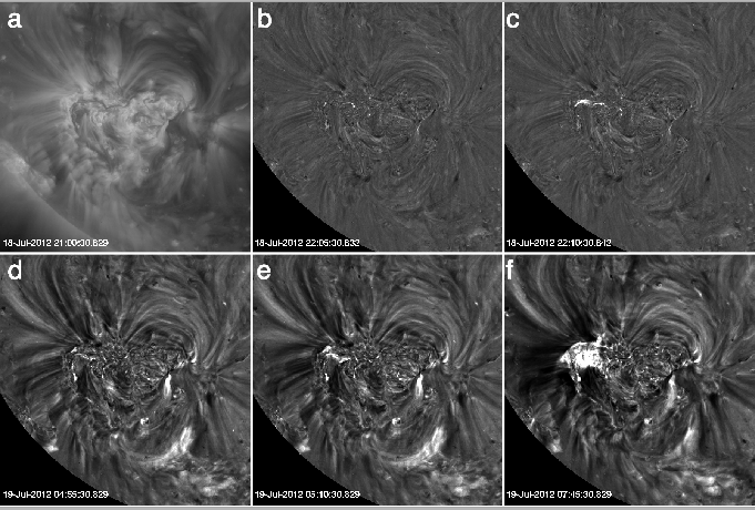
Figure 3: Evolution of AR 11520 during 2012 July 18-19 as seen by EUVI-A 195. (a) Direct image (log-scaled) of the scene. (b-c) and, (d-e) show the evolution of the flare brightenings during the confined and eruptive flares, respectively. (f) the post-eruption arcade resulting from the eruptive flare. Panels (b-f) are base-ratio images (linear scaling from 0.2-3) of the EUVI-A 195 images relative to the image in (a). The images have been differentially rotated to the time of the base image before taking the ratios. Brighter gray level correspond to higher intensities or ratios.

4. The flare brightenings map along the NL. This is easily determined by checking the EUVI-A images above the target AR (Figure 3). Comparing the shape and orientation of the NL before the eruption (Figure 3a) with the brightenings taking place during the confined flare (panels b-c), we see that the brightenings run almost parallel to the horizontal segment (’S1’). These ribbon-like brighenings correspond to the footpoints of the field lines energized by the flare. The pattern is widely consistent with flux rope formation from a sheared arcade: arcade fields with footpoints almost perpendicular to the NL are transformed (through slow shearing motions, for example) to coiled flux rope field lines connecting distant points along the NL. The final footpoints of these flux rope field lines are arranged at opposite ends of the NL running more or less parallel to it.

5. It exhibits a “half-loop” topology. A striking feature of the “core+legs” 131 structure is that only the southward part of the legs is visible (e.g., Figure 2c-d). There is no obvious extension of these legs to the north. On the other hand, the legs of the post-eruption loops, underneath the structure, are fully visible on either side of the ”X” point. This discrepancy is explained in Section 3 and provides us with a very strong indication that we are dealing with a twisted three-dimensional flux rope structure.

One may be tempted to describe the hot core observed in 131 as a “blob” or a “plasmoid”. Note that both terms arise from 2D or 2.5D depictions and imply structures partially or fully detached from the solar surface which could eventually escape the instrument’s field of view. However, the hot core is attached to the surface via the legs discussed above and does not escape from the Sun.

We emphasize here that the formation of the flux rope would have gone largely unnoticed without the hot channel observations. The warmer channels like 171, 193, or 211 (i.e., the 211 on-line movie, movie2.mp4) show only expansion and rise of loops overlying the 131 flux rope structure in phase with the expansion of the 131 flux rope structure.

To deduce the flux rope kinematics and compare it to the various emissions we manually trace the height of the flux rope front in the 131 images (Figure 4). The upper panel displays the height-time ($h-t$) measurements (square boxes). We assign a conservative error of five AIA pixels (0.003 $\mathrm{R_{\odot}}$) to every measurement. The $h-t$ data are smoothed first to reduce small-scale fluctuations. We use a smoothing cubic spline scheme (e.g., Weisberg, 2005) which minimizes a function consisting of the sum of a ${\chi}^{2}$ fit of the data with a cubic spline plus a penalty function proportional to the second derivative of the cubic spline. Five knots are found to minimize the Akaike Information Criterion (AIC) and the Bayesian Information Criterion (BIC). Both AIC and BIC are standard measures of the relative goodness of a statistical model and supply a means of model selection (e.g., Liddle, 2007). The flux rope starts to slowly rise at around 22:00 UT until around 22:20 UT, when it reaches a constant height (i.e., it ”stops” at the corresponding height). Next, we derive the evolution of flux rope speed and acceleration by taking the first and second numerical time derivatives of the smoothed $h-t$ measurements (solid and dashed black lines, respectively in Figure 4, middle panel). We then perform 1000 Monte-Carlo simulations of the (assumed) Gaussian $h-t$ uncertainties to derive the 1-$\sigma$ point-wise uncertainties for the velocity and acceleration (red and blue curves in Figure 4, middle panel).

During the impulsive rise phase the velocity reaches a peak value of $\approx$ 60 $\mathrm{{km}{s}^{-1}}$ and then decreases to $\approx$ 0 $\mathrm{{km}{s}^{-1}}$. The flux rope undergoes an asymmetric short-lived acceleration pulse with a duration of $\sim 12$ few minutes. Note we are ”missing” part of its rise phase, i.e. the acceleration does not start from zero. We attribute this to the abrupt appearance and rise of the observed structure in the first frames used in our measurements. We verified that this behavior was not due to the 1-minute cadence images we used in our analysis: we were not able to see any significant change that could be measured with some confidence before 21:59:33 UT (i.e. our first measurement point) even when browsing the full 12-s 131 data. The bottom panel of Figure 4 contains normalized curves (to their respective peak values) of: (i) GOES 1-8 Å SXR light curve (solid line), (ii) its temporal derivative (as calculated from averages over 10 full resolution temporal pixels; dashed line) which is a proxy of the Hard Xrays (HXRs) and thus a metric for the energy release rate due to flare reconnection, and (iii) the 131 light curve (dash-dot line) integrated within a box containing the flux rope as shown in Figure 2d. We focus on light curves from a small area containing the flaring region to derive a more accurate estimate for the true onset time and rise rate of the associated flare. Generally speaking, the averaging over the entire solar disk of the GOES measurements may lead to a delayed flare onset times and/or shallower rises. Comparing now the middle and lower panels of Figure 4 we find that the HXR proxy exhibits a couple of short-lived pulses with the first reaching its peak slightly after ($<$ 1 minute) the peak of the acceleration. The observed flare - flux rope dynamics largely conform with the well-known synchronization between flare emissions and CME acceleration (e.g., Zhang et al., 2001; Zhang et al., 2004; Maričić et al., 2007; Temmer et al., 2010; Bein et al., 2012). For example, the recent extensive statistical study of Bein et al. (2012) found for a set of 95 events that: (i) CME acceleration starts before the SXR flare onset (75 % events) and (ii) the time delay between the peaks of the CME acceleration and of the SXRs temporal derivative occur within $\pm$ 10 minutes (81 % of events). Our event clearly falls within these limits and delays.

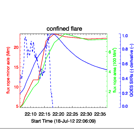
Figure 5: Evolution of the flux rope (full) minor axis (red) and of its area (green) from ellipse fittings of the 131 flux rope core for the confined flare. Normalized to their peak values GOES SXRs (blue solid line) and its temporal derivative (blue dashed line) are also displayed.

Further insight into the formation and the subsequent evolution of the flux rope can be obtained by comparing its size evolution with the dynamics of the associated flare. We manually select nine points outlining the flux rope core (avoiding the legs) for several times in 131 and then fit an ellipse to the selected points. Figure 5 shows the temporal evolution of the derived flux rope minor radius and area. Given the almost radial path followed by the flux rope, the minor (major) axis of the fitted ellipses corresponds to the lateral (radial) extent of the flux rope core. The radii and areas are first corrected for the instrumental resolution width (Table 7 in Boerner et al. (2012)).

Several remarks from Figure 5 are now in order. First, the initial size of the flux rope core is very small (e.g. initial minor axis radius of 4.7 Mm or 0.006 $\mathrm{R_{\odot}}$). Second, the minor axis and area of the flux rope core, and hence its major axis, undergo a short-lived period of strong growth starting at around 22:06 UT and lasting for 13 and 17 minutes, respectively. The two-phase development of the flux rope minor axis largely coincides with a two-phase activity (22:08 - 22:11 UT and 22:15 - 22:16 UT) seen in the GOES SXR derivative. The energy release rate, peaks two minutes before (22:16 UT) the flux rope core reaches its maximum size ($\sim 22:18$ UT). These timings strongly suggest that flare reconnection was responsible for the flux rope formation. This is corroborated further by the fact that the flux rope growth ceases within 2-3 minutes of the SXR flare peak. After $\approx$ 22:23 UT, the flux rope maintains an almost constant size, which implies that the flux rope formation is completed by this time. The flux rope also reaches its peak height at this time (upper panel of Figure 4).

The initial height ($\approx$ 27.6 Mm; Figure 4) and minor axis length $\approx$ 4.7 Mm Figure 5) of the flux rope clearly indicate that the structure was formed at coronal heights. Moreover, the flux rope structure readily attained flare temperatures. This argues in favor of the formation of a coronal flux rope.

2.2 Quasi-Static Evolution and Cooling of the Flux Rope

Once the confined flare ends at around 23 UT on July 18, the flux rope structure undergoes cooling. Starting at the same time and lasting for several hours (until around 04:00 UT on July 19) the flux rope and overlying loops begin a phase of slow rise and expansion.

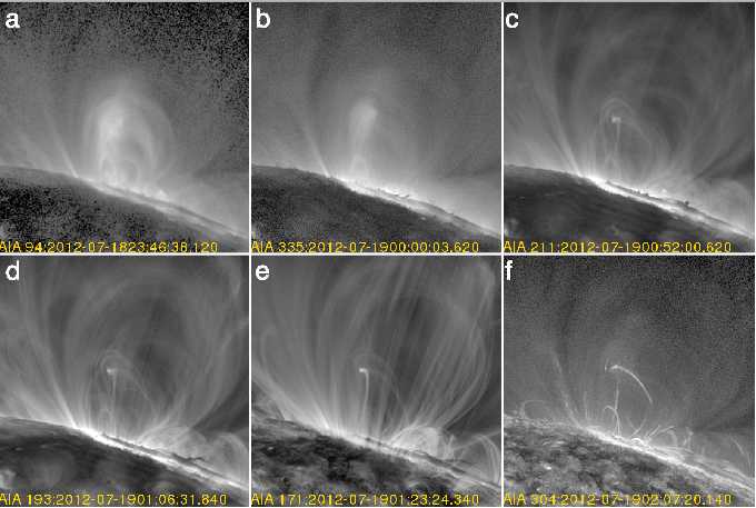
Figure 7: Cooling of the flux rope structure after the confined flare as seen in various AIA channels. The field of view is 600$\times$ 600 $\mathrm{{arcsec}^{2}}$. Images have been rotated so that their vertical dimension corresponds to the East-West direction.

The cooling of the flux rope structure evolves coherently across the different AIA channels after the end of the confined flare. Essentially the hot 131 flux rope starts to appear sequentially in AIA channels with decreasing characteristic temperatures. An example of this evolution is shown in Figure 7 where we see the flux rope core and legs appearing in the different AIA channels at different times. The core emission is stronger in the hotter channels (94 and 335) while the legs are better seen in the warmer channels (211, 193, 171, 304). Indeed, the flux rope core was visible for several hours in the 335 channel, even after the end of this phase at $\sim$ 04:00 UT on July 19, which suggests that its temperature did not drop below the characteristic temperature of 335 ($\sim 2.5$ MK). The elevated temperature likely explains the lack of a sigmoid in the EUVI-A 195 images (characteristic temperature of 1.3 MK) above the source AR. Moreover, the cooling of the flux rope progressed from its interior to its exterior, i.e. in the same sense to the heating of the flux rope during its formation. These patterns are compatible with magnetic reconnection during the confined flare adding new magnetic flux to the flux rope (e.g., Lin et al., 2004). For example,the parts of the flux rope formed earlier (the inner parts) would then cool earlier to a given temperature. The cooling of the flux rope structure leads to a very important conclusion: the magnetic structure of the flux rope was maintained for several hours after its formation during the confined flare.

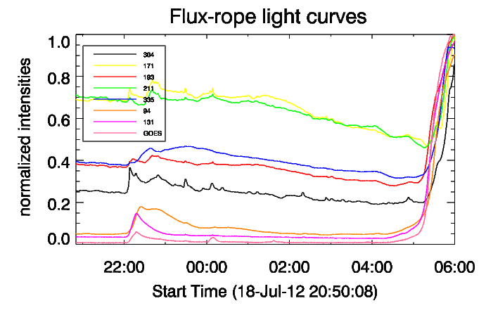
Figure 6: Light curves in various AIA channels within the box encapsulating the flux rope structure as shown in Figure 2d and in the GOES 1-8 Å  channel. All curves are normalized to their respective peak values.

The cooling of the flux rope can be also appreciated by inspecting the light curves of different AIA channels intergrated within a box containing the flux rope and shown in Figure 2d. The AIA light curves, together with the GOES 1-8 Å light curve, are displayed in Figure 6. The plot shows emission peaks in the various channels, early in the plotted timeline, with an ordering as a function of the temperature of peak response in each channel: 131$\rightarrow$94$\rightarrow$335$\rightarrow$211$\rightarrow$193$\rightarrow$171$\rightarrow$304. Additionally, we notice another emission peak in 304 occurring before the higher temperature peaks. This is probably emission from the footpoints of the flaring loops, which preceeds the emission from their coronal sections.

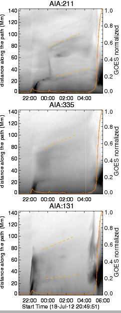
Figure 8: Stack plots of the intensity along the path shown in Figure 2d. Plots in 211, 335 and 131 are displayed in the top, middle, and bottom panel, respectively. Time increases from left to right and distance along the path increases from the bottom up. The intensity in each point is the average over a 5-pixel wide slit running perpendicularly to the path. The color table is reversed, i.e. darker shades correspond to higher intensities. The overplotted dashed lines point to a sample of the slow rise tracks.

While the flux rope cools, the AIA movies show evidence of a slow rise and expansion of the flux rope and its overlying loops. This is particularly evident in the warmer channels. The expansion continues for several hours, until about 04:00 on July 19. To better visualize and quantify the slow expansion and rise phase, we create a stack plot of the temporal evolution of the intensity, for several AIA channels, along the path shown in Figure 2d. The path contains the flux rope and overlying loops. A sample of the resulting stack plots is shown in Figure 8. First, we note a series of low-lying bright streaks around the time of the confined flare. These correspond to the flux rope observed in different channels. Second, we note a series of almost linear intensity tracks, with positive (hence rising) slopes, starting at different heights above the flux rope (dashed lines). These tracks can be seen in different channels and last from $\approx$ 00:00 to 04:00. They correspond to the slow rise of the overlying loops. The slopes of these linear tracks yield speeds in the range 0.5-2.0 $\mathrm{km\,{s}^{-1}}$. Because the magnitude of these speeds is a small fraction of the characteristic speed in the AR coronal core ($\sim 1000$ $\mathrm{km\,{s}^{-1}}$), the observed rise and expansion can be described as a quasi-static process. In addition, the solar rotation is too slow to explain the observed rise during the few hours we consider here. During this interval, and in tandem with the cooling of the flux rope and slow rise of the overlying loops, we also observe evidence of activities taking place at and around the flux rope core, including apparent displacements of its legs. The latter implies some sort of magnetic field reconfiguration.

This quasi-static rise of the overlying loops can explain a steady, slow decrease in the intensity of the warmer channels (e.g., 211, 193, 171) which starts at around 02:00 UT (see Figure 6). It is simply due to the slow evacuation of loops from our selection box.

2.3 Destabilization and Eruption of the Flux Rope

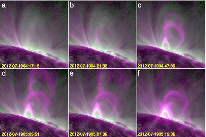
Figure 9: 131 (red) and 335 (green) color composites before and during the eruptive flare on 2012 July 19. The time tags correspond to the 335 images. The corresponding 131 images were taken 6 sec later. The field of view is 600$\times$ 600 $\mathrm{{arcsec}^{2}}$. The images have been rotated so that their vertical dimension corresponds to the East-West direction.

Starting at around 03:00 UT, the system enters into a new phase leading to the destabilization and eruption of the flux rope, a strong flare and eventually a fast CME. We post an on-line movie (movie3.mp4) showing a composite of 335-131 images from this phase. Figure 9 contains several snapshots from this movie.

Starting at around 02:47 UT, the 131 images show a cusp brightening below the initial flux rope along with the appearance of ”half-loop” structures, similarly to what was observed during the confined flare. At the same time, the 335 flux rope core is rising slowly. These motions become more pronounced from 03:57 UT onwards, when the cusp and ”half-loops” start to grow faster and the 335 flux rope rises at a faster pace (Figure 9). As discussed earlier, the existence and development of hot cusp structures points to magnetic reconnection taking place above these structures. We believe that this process is adding new flux around the erupting flux rope core. This can be seen in panels (e) and (f) of Figure 9 where we observe the 335 flux rope core ”sitting” on top of a concave upwards V-shaped 131 structure. The latter may be ”nested” around the flux rope core via magnetic reconnection above the cusp (e.g., Lin et al., 2004). The flux rope core and leg system continue to rise and the flux rope core exits the AIA FOV at 05:07 UT. Note here that the SXR levels were relatively low (less than $\approx$ B3 of the GOES scale) during these evolutions. The associated flare is still at its gradual rise phase when the flux rope core exits the AIA FOV. Around 05:36 UT a WL CME emerges in the LASCO C2 coronagraph. The CME is a typical flux rope CME (see for example the bottom left image of Figure 1 and Vourlidas et al. (2012a) for definitions). The CME front exits the C2 FOV at around 06:00 UT when the associated M7.7 GOES class flare reaches its peak. We thus conclude that the flux rope rise described above leads to an eruption, i.e. we are dealing here with an eruptive flare.

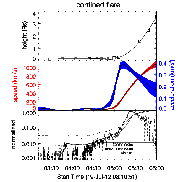
Figure 10: Eruptive flare. Top: temporal evolution of the flux rope height from measurements in the 335 Å  channel of AIA and LASCO C2 (squares; the last three data points correspond to LASCO measurements). The associated uncertainties are too small to be seen in this scale. The heights resulting from the application of a smoothing cubic spline to the original measurements are shown with a solid black line. Middle: first (velocity) and second (acceleration) temporal derivatives of the smoothed height points (solid and dashed black lines respectively). Point-wise 1-$\sigma$ uncertainties in the velocity (red) and acceleration (blue) from 1000 Monte-Carlo simulations of the (assumed) Gaussian $h-t$ uncertainties are also shown. Bottom: normalized light curves of the GOES 1-8 Å  flux (solid line), its temporal derivative (dashed line) and the 131 light curve of the box encapsulating the flux rope structure in Figure 2d (dashed-dotted line).

As we did in the case of the confined flare, we deduce the kinematics of the eruptive flux rope and compare them with the associated flare dynamics. We manually track the front of the erupting flux rope in the 335 images to determine the $h-t$ profile (upper panel of Figure 10). These measurements are complemented by the $h-t$ of the resulting WL CME core observed in LASCO C2 (the last 3 datapoints in the upper panel of Figure 10). An uncertainty of 5 pixels (0.043 $\mathrm{R_{\odot}}$) is assigned to the LASCO measurements. The same smoothing cubic spline scheme used for the confined flare measurements, this time with seven knots, is applied to the $h-t$ measurements to obtain a smoothed $h-t$ profile. The first and second temporal derivatives provide the flux rope velocity and acceleration, respectively. The derived speed and acceleration profiles along with their point-wise 1-$\sigma$ uncertainties from 1000 Monte-Carlo simulations of the (assumed) Gaussian $h-t$ uncertainties are displayed in the middle panel of Figure 10. Finally the lower panel contains the GOES 1-8 Å light curve, its temporal derivative and the 131 light curve over the box shown in Figure 2d.

Figure 10 leads to the following remarks. The flux rope moves relatively slowly in the AIA FOV, reaching a maximum speed of $\approx$ 100 $\mathrm{km\,{s}^{-1}}$. The bulk of its acceleration occurs beyond the AIA FOV where the flux rope speed exceeds 1000 $\mathrm{km\,{s}^{-1}}$. The flux rope eruption leads to a fast CME. The flux rope acceleration rise consists of two phases: a gradual rise ($\approx$ 04:40-04:55 UT) followed by an impulsive rise. The acceleration reaches its peak at 5:10 UT. Similarly, the associated flare (GOES SXRs and 131 light-curves) exhibits a gradual rise ($\approx$ 04:15-05:05 UT) followed by an impulsive rise phase ($\approx$05:05-05:25 UT). The flare energy release rate (temporal derivative of GOES SXRs) evolves very similarly to the CME acceleration, exhibiting a gradual and impulsive phase and reaches its peak at around 05:25 UT.

The above findings suggest a tight correspondance between flare heating and CME acceleration, as has been found already for the majority of CMEs and also for the confined flare (see the detailed discussion of CME-flare timings from statistical studies in Section 2.1). However, (i) the impulsive rise of the acceleration starts around 10 minutes before the start of the impulsive rise of the flare, and (ii) the peak of the acceleration occurs around 10 minutes before the peak of the SXR temporal derivative. We note here that the exact timings between the CME impulsive acceleration and flare emissions are somehow uncertain because the bulk of the CME impulsive acceleration takes place between the outer edge of the AIA FOV and the inner edge of the C2 FOV, where measurements are unavailable. In the next sections, we focus on the important implications of the time delays discussed above with respect to the possible eruption trigger.

3 3D context of the Event

So far, we focused on the interpretation of the AIA observations only. We believe that they provide a very convincing case for the formation and subsequent eruption of a magnetic flux rope based on the observed morphology, association with hot cusp-like loops, and temperature evolution in the various AIA channels. Most of these results are possible because of the fortuitous alignment of the flux rope axis parallel to the AIA LOS thus providing an almost cartoon-like view of the structure. At the same time, the single viewpoint AIA observations cannot address the 3D configuration and low atmosphere conectivity of the structure because these connections are hidden behind the limb.

Thankfully, we can take advantage of the EUVI-A 195 images which record a top view of the whole AR. Although SECCHI lacks a dedicated hot channel like the AIA 131, the 195 passband includes contributions from a Fe XXIV line at 192 Å  with peak temperature of 16 MK. It can also be compared rather directly with the AIA 193 images. Indeed, using the AIA images as a guide, the flux rope can be barely identified as a faint loop structure. The emission in the EUVI-A images, however, is dominated by brightenings on either side of the NL, mostly lying along the southern boundary, away from Earth (Figure 3. We will focus on these brigtnenings for our analysis because they play an important role in deriving the 3D configuration of the flux rope as we will see shortly.

First, we recall the unsual AIA observations of the half-legs in Figure 2c-e. Both sides of the flare loops are clearly visible while the flux rope core appears threaded by two distinct loop bundles with a single footpoint originating at some distance from the flaring loops. In other words, we have three footpoint clusters somewhere south of the NL and a single footpoint cluster northward of the NL. Why is that and what are those half-loops threading the flux rope?

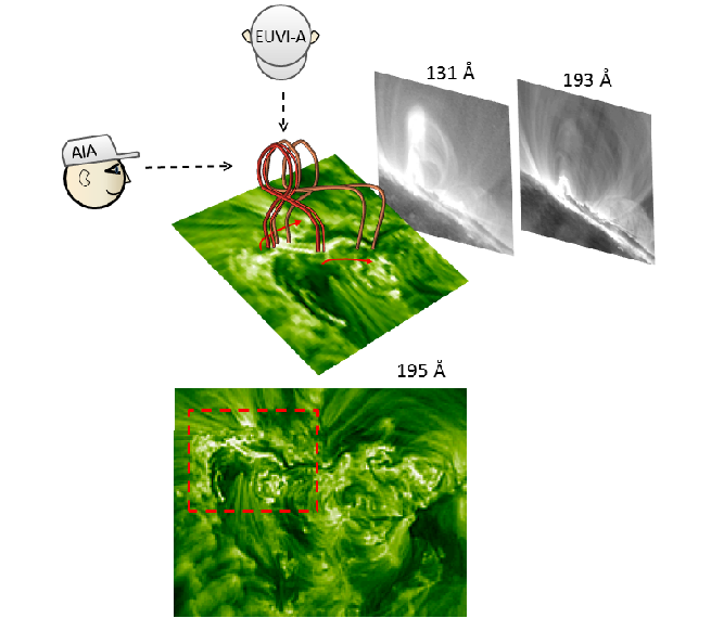
Figure 11: The proposed 3D configuration of the flux rope. The flux rope structure is represented by a few hypothesized field lines (red and orange curves) that conform to the views from above (EUVI-A 195) and from the side (AIA 131 and 193). The red arrows show the progression of the brightenings along the surface and the red dotted-line box marks the area shown in detail at the center of the figure.

The answer lies in the EUVI-A images taken at 22:10 UT (Figure 3c) almost simultaneously to the AIA 131 images in Figure 2c. The EUVI-A image shows three distinct brightening areas. The most extended is the easternmost one which corresponds to the flaring loop (and flux rope) seen from above. The other two areas must be, therefore, the footpoints of the two loops bundles that thread the flux rope. The separation probably explains the gap between the two bundles as seen by AIA. The lack of any other significant brightenings, north of the NL, means the loops originating in all three southern locations must connect back along the easternmost footpoint. The concentration of all these field lines and half-loop appearance for the two core bundles can then be explained by a kinked configuration where the kinked loops form the flux rope viewed in AIA with their axis predominanlty parallel to the AIA LOS. We summarize the resulting 3D configuration in Figure 11 where we plot the AIA 131 and 193 images and the closest in time EUVI-A 195 image as viewed from the two perspectives. We then draw our proposed 3D representation of a few field lines that is consistent with the observations from the two viewpoints. Patsourakos et al. (2010a) deduced a similar configuration in another event based on detailed 3D analysis although they lacked the high cadence and temperature coverage of the AIA instrument. Ji et al. (2003); Alexander et al. (2006); Török & Kliem (2005) reported on very clearly kinked prominences which were also failed eruptions. Our interpretation in Figure 11, therefore, does not seem unreasonable. It does imply, however, that a kinked flux rope can survive for quite some time (at least 6 hours) before erupting.

4 Discussion

In this work, we present the first direct unambiguous evidence of a pre-existing flux rope involved in a fast CME eruption. Thanks to EUV observations in many passbands and from two viewpoints, we can follow the temporal and spatial evolution of the system in great detail. To recap, we first present a brief event timeline with the approximative times of the most important aspects of our observations, with the entire sequnece running from 22:00 UT on 18 July until 05:36 on 19 July 2012.

• 22:00-22:30. A magnetic flux rope is formed during a confined flare.

• 22:30-02:10. The flux rope plasma cools appearing sequentially in EUV channels with peak temperatures ranging from flaring to transition region conditions.

• 22:30-04:00. The flux rope and overlying coronal structures undergo a phase of slow quasi-static rise (speed 0.5-2 $\mathrm{km\,{s}^{-1}}$) and expansion.

• 02:47-03:57. a hot cusp loop structure and new legs threading the flux rope appear in the 131 channel only.

• 04:45-05:36. the flux rope begins to impulsively accelerate and a WL CME appears.

4.1 Event Sequence Scenario

In the previous sections, we split the flux rope evolution in three phases (formation, quasi-static rise and expansion, and eruption). We now incorporate them into a coherent physical scenario which involves ideal and non-ideal physical processes.

1. Flux rope formation The observations supply strong evidence that the flux rope is formed via magnetic reconnection during the confined flare. The evidence includes the simultaneous formation of cusp-like loops below the flux rope with flare temperatures, the tight synchronization between the flare energy release and the evolution of the flux rope size, and the distribution of flare brightenings along the NL. The high initial altitude and size of the flux rope points to a coronal flux rope. Overall, the observations point to the conversion of arcade magnetic fields via successive reconnections to flux rope helical fields. This mechanism of flux rope formation is addressed in a number of theoretical, modeling, and observational works (e.g., van Ballegooijen & Martens, 1989; Moore & Roumeliotis, 1992; Low, 1996; Antiochos et al., 1999; Amari et al., 2000; Lin et al., 2004; Lynch et al., 2008; Vršnak, 2008; Green & Kliem, 2009; Georgoulis, 2011) which our observations are now verifying.

2. Slow quasi-static rise It is well established that slow photospheric footpoint motions leading to shearing and/or twisting can drive the slow rise and inflation of coronal structures. This mechanism can be purely ideal, i.e. not associated with magnetic reconnection, and can explain, in principle, the observed quasi-static rise of the flux rope and overlying corona. However, we observe the formation of a cusp structure along with ”half-loop” legs threading the flux rope core starting at around 02:47 UT during this phase. This clearly suggests that low reconnection-rate phenomena are taking place. Moreover, the confined flare and coronal flux rope exhibit an ”X”-type topology. We therefore suggest that small magnitude tether-cutting reconnections may be transforming arcade fields into flux rope fields causing the growth and slow rise of the initial flux rope. This process could be essentialy the same process responsible for the flux rope formation in the previous paragraph but occurring with lower magnitudes of the related phenomena. The cause of the slow rise observed before 02:47 UT is less certain.

3. Magnetic seed and trigger of the fast CME The ’seed’ for the fast CME on July 19 was the destabilization of the pre-existing flux rope formed almost seven hours prior to the onset of the impulsive acceleration phase of the CME. The delay in the onset of the SXR impulsive phase and in the peak of the SXR temporal derivative with respect to the onset and peak of the flux rope acceleration (see Figure 10 and corresponding discussion) points to a flux-rope (i.e. ideal) instability for the trigger of the eruption. In other words the strong acceleration of the plasma starts before the strong flare heating. The kink (e.g., Török & Kliem, 2005) and torus instabilities (e.g., KliemTörök, 2006) are two commonly invoked flux rope instabilities for the trigering of CMEs. However, the lack of hard evidence of flux rope rotation during the eruption, which could have served as an indication of kink instability, suggest we can probably exclude this instability as the trigger of the eruption. On the other hand, the slow and long duration quasi-static rise of the flux rope could have lifted it to altitudes where the overlying constraining magnetic field gradients are stronger, thus facilitating the onset of the torus instability as discussed in a number of series of recent MHD modeling investigations (e.g., Aulanier et al., 2010; Fan, 2010; Savcheva et al., 2012). Mechanical loss of equilibrium of a flux rope once it reaches a critical height (e.g., Forbes & Isenberg, 1991; Forbes, 2000; Vršnak, 2008) is another possible trigger for the observed eruption.

To summarize, the above scenario contains both ideal and non-ideal processes with the ideal processes possibly triggering the eruption while the non-ideal processes are responsible for the flux rope formation and its subsequent slow quasi-static rise.

4.2 Implications for CME Initiation

For the first time, we have confirmation that truly pre-existing hot coronal flux ropes exist and can be long-lived. Note that previous observations detected a hot flux rope forming only a few minutes before the onset of the associated eruption (Cheng et al., 2011; Zhang et al., 2012). The very significant span of almost seven hours between the flux rope formation and its eruption underlines the importance of studying the long-term evolution of ARs and to not only concentrate on the immediate time around the eruption. We believe that we would have reached significantly different, possibly erroneous, conclusions regarding the onset of the CME on July 19 had we focused only on the events surrounding the CME onset. We are also in the position to explain the rarity of past detections of pre-existing flux ropes: (1) Lack of high cadence EUV imaging observations in flare temperatures prior to AIA. (2) Small spatial (horizontal and vertical) and temporal scales of the flux rope requiring high spatial resolution. (3) Favorable line of sight orientation with respect to the flux rope axis. The initially small spatial scales require that the flux rope is situated right at the limb so that it would be vissible before its destabilization and rapid ascent. All of these requirements were met by our observations.

Our study also supplies tight constraints for models of flux rope formation and eruption. The flux rope was formed in a period of $\approx$ 20 minutes. The flux rope was a rather small structure during its formation. Its initial (final) minor and major axis had lengths of $\approx$ 4.7 (22.2) and 9 (41.5) Mm, respectively. Moreover, the flux rope evolved within a small range of heights, $\approx$ 80 Mm at the end of the confined flare and 138 Mm at the start of the impulsive CME acceleration. The period of slow quasi-static rise lasted for almost seven hours. Therefore, succssful flux rope models need to reproduce rapidly formed small and low-lying coronal flux ropes with long quasi-static intervals before eruption.

The present work suggests that the events taking place during confined flares may play an important role in, at least some, solar eruptions. The magnetic field reconfiguration associated with the confined flare in this event could be considered as a catalyst for the sequence of events leading to the CME. It did not only create the flux rope which was the seed for the CME but it also re-configured the field by the formation and initial rise of the rope by setting up a topology (i.e., X-point) which favors (coronal) magnetic reconnection. We note here that large numbers of small magnitude confined flares may take place in the source AR before, and after, major solar eruptions and eruptive flares (e.g., M and X class). Such small magnitude events may release only part of the accumulated free energy in the form of radiation while some portion of the free energy ends up as magnetic energy of a flux rope. A similar picture of flux rope formation by small/confined flares was theoretically formulated by Low (1996). Indeed, inspection of the evolution of our AR over the long interval of 2012 July 17-20 gives some hints of a homologous behavior with a few confined flares giving rise to flux-rope like structures. Evidently, the LOS orientation was not as optimal as for the event on July 18. In addition, all flaring and eruptive activity seems to originate from around the same location along the NL. Obviously our hypothesis about the overall role of confined flares in the formation and initiation of CMEs requires further testing against more observations.

Regarding future instrumentation for addressing the CME initiation problem, our study makes it clear that a coronagraphic capability in flare EUV lines withing the inner corona ($<1.5$ $\mathrm{R_{\odot}}$) may be an important element of a mission on Solar Eruptive Events. Such observations will allow us to trace the hot flux rope as far as possible in the low corona, and avoid the strong footpoint emissions and image saturation and diffraction effects from the associated flares which may mask the faint flux rope emissions in current telescopes. An obvious logical extension of this study is a survey of the AIA database for more eruptive events to access how common hot pre-existing (or otherwise) flux ropes are and how and when do they form and eventually erupt.

References

- Alexander et al. (2006) Alexander, D., Liu, R., & Gilbert, H. R. 2006, ApJ, 653, 719
- Amari et al. (2000) Amari, T., Luciani, J. F., Mikic, Z., & Linker, J. 2000, ApJ, 529, L49
- Antiochos et al. (1999) Antiochos, S. K., DeVore, C. R., & Klimchuk, J. A. 1999, ApJ, 510, 485
- Archontis & Hood (2008) Archontis, V., & Hood, A. W. 2008, ApJ, 674, L113
- Aschwanden et al. (2011) Aschwanden, M. J., Boerner, P., Schrijver, C. J., & Malanushenko, A. 2011, Sol. Phys., 384
- Aulanier et al. (2010) Aulanier, G., Török, T., Démoulin, P., & DeLuca, E. E. 2010, ApJ, 708, 314
- Aurass et al. (1999) Aurass, H., Vršnak, B., Hofmann, A., & Rudžjak, V. 1999, Sol. Phys., 190, 267
- Bein et al. (2012) Bein, B. M., Berkebile-Stoiser, S., Veronig, A. M., Temmer, M., & Vrasnk, B. 2012, ApJ, 755, 44
- Boerner et al. (2012) Boerner, P., Edwards, C., Lemen, J., et al. 2012, Sol. Phys., 275, 41
- Brueckner et al. (1995) Brueckner, G. E., Howard, R. A., Koomen, M. J., et al. 1995, Sol. Phys., 162, 357
- Canfield et al. (1999) Canfield, R. C., Hudson, H. S., & McKenzie, D. E. 1999, Geophys. Res. Lett., 26, 627
- Canou et al. (2009) Canou, A., Amari, T., Bommier, V., et al. 2009, ApJ, 693, L27
- Carmichael (1964) Carmichael, H. 1964, NASA Special Publication, 50, 451
- Chen et al. (2006) Chen, J., Marqué, C., Vourlidas, A., Krall, J., & Schuck, P. W. 2006, ApJ, 649, 452
- Chen (2011) Chen, P. F. 2011, Living Reviews in Solar Physics, 8, 1
- Cheng et al. (2011) Cheng, X., Zhang, J., Liu, Y., & Ding, M. D. 2011, ApJ, 732, L25
- Dove et al. (2011) Dove, J. B., Gibson, S. E., Rachmeler, L. A., Tomczyk, S., & Judge, P. 2011, ApJ, 731, L1
- Fan (2010) Fan, Y. 2010, ApJ, 719, 728
- Forbes & Isenberg (1991) Forbes, T. G., & Isenberg, P. A. 1991, ApJ, 373, 294
- Forbes (2000) Forbes, T. G. 2000, J. Geophys. Res., 105, 23153
- Fuller et al. (2008) Fuller, J., Gibson, S. E., de Toma, G., & Fan, Y. 2008, ApJ, 678, 515
- Georgoulis (2011) Georgoulis, M. K. 2011, IAU Symposium, 273, 495
- Gibson et al. (2006) Gibson, S. E., Foster, D., Burkepile, J., de Toma, G., & Stanger, A. 2006, ApJ, 641, 590
- Gibson & Fan (2006) Gibson, S. E., & Fan, Y. 2006, ApJ, 637, L65
- Green & Kliem (2009) Green, L. M., & Kliem, B. 2009, ApJ, 700, L83
- Green et al. (2011) Green, L. M., Kliem, B., & Wallace, A. J. 2011, A&A, 526, A2
- Engvold (1989) Engvold, O. 1989, Dynamics and Structure of Quiescent Solar Prominences, 150, 47
- Hirayama (1974) Hirayama, T. 1974, Sol. Phys., 34, 323
- Howard et al. (2008) Howard, R. A., Moses, J. D., Vourlidas, A., et al. 2008, Space Sci. Rev., 136, 67
- Hudson et al. (1999) Hudson, H. S., Acton, L. W., Harvey, K. L., & McKenzie, D. E. 1999, ApJ, 513, L83
- Huang et al. (2011) Huang, J., Démoulin, P., Pick, M., et al. 2011, ApJ, 729, 107
- KliemTörök (2006) Kliem, B., Török, T. 2006, Physical Review Letters, 96, 255002
- Klimchuk (2001) Klimchuk, J. A. 2001, Space Weather (Geophysical Monograph 125), ed. P. Song, H. Singer, G. Siscoe (Washington: Am. Geophys. Un.), 143 (2001), 125, 143
- Kopp & Pneuman (1976) Kopp, R. A., & Pneuman, G. W. 1976, Sol. Phys., 50, 85
- Koutchmy et al. (2004) Koutchmy, S., Baudin, F., Bocchialini, K., et al. 2004, A&A, 420, 709
- Kucera et al. (2012) Kucera, T. A., Gibson, S. E., Schmit, D. J., Landi, E., & Tripathi, D. 2012, ApJ, 757, 73
- Lemen et al. (2012) Lemen, J. R., Title, A. M., Akin, D. J., et al. 2012, Sol. Phys., 275, 17
- Liddle (2007) Liddle, A. R. 2007, MNRAS, 377, L74
- Ji et al. (2003) Ji, H., Wang, H., Schmahl, E. J., Moon, Y.-J., & Jiang, Y. 2003, ApJ, 595, L135
- Lin et al. (2004) Lin, J., Raymond, J. C., & van Ballegooijen, A. A. 2004, The Astrophysical Journal, 602, 422–435
- Li et al. (2012) Li, X., Morgan, H., Leonard, D., & Jeska, L. 2012, ApJ, 752, L22
- Liu et al. (2010) Liu, R., Liu, C., Wang, S., Deng, N., & Wang, H. 2010, ApJ, 725, L84
- Lynch et al. (2008) Lynch, B. J., Antiochos, S. K., DeVore, C. R., Luhmann, J. G., & Zurbuchen, T. H. 2008, ApJ, 683, 1192
- Low (1996) Low, B. C. 1996, Sol. Phys., 167, 217
- Magara & Longcope (2001) Magara, T., & Longcope, D. W. 2001, ApJ, 559, L55
- Manchester et al. (2004) Manchester, W., IV, Gombosi, T., DeZeeuw, D., & Fan, Y. 2004, ApJ, 610, 588
- Maričić et al. (2007) Maričić, D., Vršnak, B., Stanger, A. L., et al. 2007, Sol. Phys., 241, 99
- Moore & Roumeliotis (1992) Moore, R. L., & Roumeliotis, G. 1992, IAU Colloq. 133: Eruptive Solar Flares, 399, 69
- Moore et al. (2001) Moore, R. L., Sterling, A. C., Hudson, H. S., & Lemen, J. R. 2001, ApJ, 552, 833
- Moore et al. (2007) Moore, R. L., Sterling, A. C., & Suess, S. T. 2007, ApJ, 668, 1221
- Patsourakos et al. (2010a) Patsourakos, S., Vourlidas, A., & Kliem, B. 2010, A&A, 522, A100
- Patsourakos et al. (2010b) Patsourakos, S., Vourlidas, A., & Stenborg, G. 2010, ApJ, 724, L188
- Plunkett et al. (2000) Plunkett, S. P. et al. 2000, Sol. Phys., 194, 371
- Régnier et al. (2011) Régnier, S., Walsh, R. W., & Alexander, C. E. 2011, A&A, 533, L1
- Reeves & Moats (2010) Reeves, K. K., & Moats, S. J. 2010, ApJ, 712, 429
- Reeves & Golub (2011) Reeves, K. K., & Golub, L. 2011, ApJ, 727, L52
- Reeves et al. (2012) Reeves, K. K., Gibson, S. E., Kucera, T. A., Hudson, H. S., & Kano, R. 2012, ApJ, 746, 146
- Robbrecht et al. (2009) Robbrecht, E., Patsourakos, S., & Vourlidas, A. 2009, ApJ, 701, 283
- Romano et al. (2003) Romano, P., Contarino, L., & Zuccarello, F. 2003, Sol. Phys., 214, 313
- Rust & LaBonte (2005) Rust, D. M., & LaBonte, B. J. 2005, ApJ, 622, L69
- Savage et al. (2010) Savage, S. L., McKenzie, D. E., Reeves, K. K., Forbes, T. G., & Longcope, D. W. 2010, ApJ, 722, 329
- Savcheva & van Ballegooijen (2009) Savcheva, A., & van Ballegooijen, A. 2009, ApJ, 703, 1766
- Savcheva et al. (2012) Savcheva, A., Pariat, E., van Ballegooijen, A., Aulanier, G., & DeLuca, E. 2012, ApJ, 750, 15
- Scherrer et al. (2012) Scherrer, P. H., Schou, J., Bush, R. I., et al. 2012, Sol. Phys., 275, 207
- Stenborg et al. (2008) Stenborg, G., Vourlidas, A., & Howard, R. A. 2008, ApJ, 674, 1201
- Sturrock (1966) Sturrock, P. A. 1966, Nature, 211, 695
- Su et al. (2010) Su, Y., van Ballegooijen, A., & Golub, L. 2010, ApJ, 721, 901
- Temmer et al. (2010) Temmer, M., Veronig, A. M., Kontar, E. P., Krucker, S., & Vršnak, B. 2010, ApJ, 712, 1410
- Török & Kliem (2005) Török, T., & Kliem, B. 2005, ApJ, 630, L97
- Tripathi et al. (2009) Tripathi, D., Kliem, B., Mason, H. E., Young, P. R., & Green, L. M. 2009, ApJ, 698, L27
- Tsuneta et al. (1992) Tsuneta, S., Hara, H., Shimizu, T., et al. 1992, PASJ, 44, L63
- Tsuneta (1997) Tsuneta, S. 1997, ApJ, 483, 507
- van Ballegooijen & Martens (1989) van Ballegooijen, A. A., & Martens, P. C. H. 1989, ApJ, 343, 971
- Vásquez et al. (2010) Vásquez, A. M., Frazin, R. A., & Manchester, W. B., IV 2010, ApJ, 715, 1352
- Vourlidas et al. (2010) Vourlidas, A., Howard, R. A., Esfandiari, E., et al. 2010, ApJ, 722, 1522
- Vourlidas et al. (2012a) Vourlidas, A., Lynch, B. J., Howard, R. A., & Li, Y. 2012, arXiv:1207.1599
- Vourlidas et al. (2012b) Vourlidas, A., Syntelis, P., & Tsinganos, K. 2012, Sol. Phys., 27
- Vrsnak et al. (1991) Vrsnak, B., Ruzdjak, V., & Rompolt, B. 1991, Sol. Phys., 136, 151
- Vrsnak (2003) Vrsnak, B. 2003, Energy Conversion and Particle Acceleration in the Solar Corona, 612, 28
- Vršnak et al. (2004) Vršnak, B., Maričić, D., Stanger, A. L., & Veronig, A. 2004, Sol. Phys., 225, 355
- Vršnak et al. (2007) Vršnak, B., Maričić, D., Stanger, A. L., et al. 2007, Sol. Phys., 241, 85
- Vršnak (2008) Vršnak, B. 2008, Annales Geophysicae, 26, 3089
- Wang & Stenborg (2010) Wang, Y.-M., & Stenborg, G. 2010, ApJ, 719, L181
- Weisberg (2005) Weisberg, S. 2005, Applied linear regression (John Wiley and Sons)
- Williams et al. (2005) Williams, D. R., Török, T., Démoulin, P., van Driel-Gesztelyi, L., & Kliem, B. 2005, ApJ, 628, L163
- Wuelser et al. (2004) Wuelser, J., et al. 2004, in Society of Photo-Optical Instrumentation Engineers (SPIE) Conference Series, Vol. 5171, Society of Photo-Optical Instrumentation Engineers (SPIE) Conference Series, ed. S. Fineschi & M. A. Gummin, 111–122
- Zhang et al. (2001) Zhang, J., Dere, K. P., Howard, R. A., Kundu, M. R., & White, S. M. 2001, ApJ, 559, 452
- Zhang et al. (2004) Zhang, J., Dere, K. P., Howard, R. A., & Vourlidas, A. 2004, ApJ, 604, 420
- Zhang et al. (2012) Zhang, J., Cheng, X., & Ding, M.-D. 2012, Nature Communications, 3,