Constrained metric variations and emergent equilibrium surfaces

Abstract

Any surface is completely characterized by a metric and a symmetric tensor satisfying the Gauss-Codazzi-Mainardi equations (GCM), which identifies the latter as its curvature. We demonstrate that physical questions relating to a surface described by any Hamiltonian involving only surface degrees of freedom can be phrased completely in terms of these tensors without explicit reference to the ambient space: the surface is an emergent entity. Lagrange multipliers are introduced to impose GCM as constraints on these variables and equations describing stationary surface states derived. The behavior of these multipliers is explored for minimal surfaces, showing how their singularities correlate with surface instabilities.

I Introduction

Surfaces occur as approximations of physical systems at almost all energy scales Nelson . More often than one would expect the only relevant degrees of freedom are the ones associated with the geometric configuration of the surface itself and its behavior is described completely by a Hamiltonian or an action constructed using the geometrical invariants of this surface. This may be something as simple as the area–representing the energy of an interface or a soap film Soap –or its relativistic analogue which represents the area of the worldsheet swept out in the course of the evolution of a string, be it a fundamental extended object or–more conservatively–some effective description of onePolyakov ; Strings .
Typically the Hamiltonian defined on a surface, $\Gamma:\{u^{1},u^{2}\}\rightarrow\mathbf{X}(u^{1},u^{2})$, is constructed by forming suitable scalars using the induced metric $g_{ab}$, the curvatures $K_{ab}$ and their covariant derivatives:

$$H=\int dA\,{\cal H}[g_{ab},K_{ab}]\,;$$ (1)

for simplicity, we consider only surfaces embedded in three-dimensional Euclidean space, $\mathbb{E}^{3}$. The important point is that the functions $\mathbf{X}$ tend not to appear explicitly in $H$. Surface area with ${\cal H}=1$, depending on the metric through its determinant, $dA=d^{2}u\,\sqrt{g}$, is the simplest example. If the tensors $g_{ab}$ and $K_{ab}$ in Eq. (1) are to represent a surface, however, they will need to be consistent with the Gauss-Codazzi (GC) and Codazzi-Mainardi (CM) equations,

$${\cal G}=0\,,\quad{\cal C}_{a}=0\,,$$ (2)

where

$${\cal G} := {\cal R}-K^{2}+K_{ab}K^{ab}\,;$$ (3a)

$${\cal C}_{a} := \nabla^{b}\left(K_{ab}-g_{ab}K\right)\,,$$ (3b)

which occur as integrability conditions on the structure equations defining how the unit tangents and normals rotate as one moves along the surface. Here $\nabla_{a}$ is the covariant derivative compatible with $g_{ab}$; ${\cal R}$ is the corresponding Ricci scalar curvature and $K$ represents the trace of $K^{a}_{\phantom{a}b}$, $K=g^{ab}K_{ab}$. Conversely, one of the corner pieces of nineteenth century geometry is the assertion that any two tensor fields, $g_{ab}$ and $K_{ab}$, satisfying Eqs. (2) will represent some surface $\mathbf{X}$, with induced metric $g_{ab}$ and extrinsic curvature $K_{ab}$, unique up to Euclidean motions Spivak . This will also be crucial. Indeed, even if $H$ depended only on the metric, this metric knows there is an extrinsic curvature tagging along.
In this Letter, we will show that it is always possible to rephrase the variational properties of surfaces in terms of a theory of gravity involving a metric, coupled to an auxiliary field $K_{ab}$, without any explicit reference to the embedding functions themselves: the surface itself is an emergent entity. In this framework Eqs. (2) are enforced by introducing Lagrange multipliers, which permits one to treat these two tensors as independent variables.
This approach contrasts dramatically with the familiar approach in terms of harmonic maps Polyakov ; Eels , or its natural extension–when curvatures are involved–in terms of auxiliary variables auxil : here, the surface does not materialize until these constraints are applied. A comparison between this framework and the latter is presented in Appendix A. Relevant antecedents motivating this work can be found in Barbour, Foster and Ó Murchadha’s “Relativity without relativity” Murchadha , Sorkin’s treatment of field theory in Minkowski space Sorkin , or Lomholt and Miao’s discussion of the ambiguities associated with the GCM equations Lomholt . It also shares features with the framework, developed in Paperfold in the context of paper folding, for enforcing local geometrical constraints.
A peculiarity of two-dimensional surfaces is that the multipliers assemble into a spatial vector field. If $H$ depends only on the intrinsic geometry, this vector field can be identified in equilibrium as a generator of surface isometries; if $H$ depends also on the curvature $K_{ab}$, on the other hand, it is identified with a conformal transformation. The role of the multipliers themselves, however, is not to displace the surface. This identification is a two-dimensional accident: they represent the strength of the interaction coupling the tensor field $K_{ab}$ to the metric on the Riemannian manifold in the formation of the equilibrium surface. The surface Euler-Lagrange equations are derived by examining the flows generated by this vector field. Its behavior will be explored in detail for area minimizing surfaces. In the case of a catenoid bridging two rings, the relevant isometry will be identified explicitly, and the connection between the singularities in this vector field and the presence of instabilities emphasized. This framework appears to provide a new approach to analyzing the instability of equilibrium surfaces.

II Surface variational principles without surfaces

Consider the following effective action or energy

$$H_{C}[g_{ab},K_{ab},\Lambda,\lambda^{a}] = H[g_{ab},K_{ab}]\,$$ (4)

$$+ I[g_{ab},K_{ab},\Lambda,\lambda^{a}]\,,$$

where

$$I=\frac{1}{4}\int dA\,\Lambda\,{\cal G}+\frac{1}{2}\int dA\,\lambda^{a}{\cal C}_{a}\,.$$ (5)

The Lagrange multipliers fields $\Lambda$ and $\lambda^{a}$ enforce the GC and CM equations, Eqs. (2), as constraints on the variables $g_{ab}$ and $K_{ab}$. In Eq. (4) one is now free to treat $g_{ab}$ and $K_{ab}$ as independent variables. The variation of $H_{C}$ is given by

$$\delta H_{C} = \int dA\,\left(-\frac{1}{2}(T^{ab}+{\cal T}^{ab})\,\delta g_{ab}+(H^{ab}+{\cal H}^{ab})\,\delta K_{ab}\right)$$ (6)

$$+ \int dA\,\nabla_{a}Q^{a}\,,$$

where the manifestly symmetric second rank tensors $T^{ab}$ and $H^{ab}$, are associated with the variation of $H$ with respect to $g_{ab}$ and $K_{ab}$; ${\cal T}^{ab}$ and ${\cal H}^{ab}$ are their counterparts for the constraining term $I$:

$$T^{ab} =-2\frac{\delta H}{\delta g_{ab}}\,, \quad{\cal T}^{ab} =-2\frac{\delta I}{\delta g_{ab}}\,;$$ (7a)

$$H^{ab} =\frac{\delta H}{\delta K_{ab}}\,, \quad{\cal H}^{ab} =\frac{\delta I}{\delta K_{ab}}\,.$$ (7b)

In Eq. (6) $Q^{a}$ represents all of the terms that have been collected in a divergence after integration by parts.

The Euler-Lagrange equations for $g_{ab}$ and $K_{ab}$ describing the equilibrium states of the surface are given respectively by:

$$T^{ab}+{\cal T}^{ab} = 0\,;$$ (8a)

$$H^{ab}+{\cal H}^{ab} = 0\,,$$ (8b)

supplemented with Eqs. (2). Eqs. (8) are analogues of the Einstein equations in general relativity. The technicalities of the variations with respect to $g_{ab}$ and $K_{ab}$ are themselves straightforward (see, for example MTWetc ). One identifies

$${\cal T}^{ab} = -\frac{1}{2}\left(\nabla^{a}\nabla^{b}-g^{ab}\nabla^{2}+{\cal R}^{ab}\right)\Lambda$$ (9a)

$$+ \frac{1}{2}\left[\nabla^{a}(\lambda^{c}K^{b}_{\phantom{b}c})+\nabla^{b}(\lambda^{c}K^{a}_{\phantom{a}c})\right]$$

$$- \frac{1}{2}\nabla_{c}\left[\lambda^{c}K^{ab}+g^{ab}\lambda^{d}K^{c}_{\phantom{c}d}\right]\,;$$

$${\cal H}^{ab} = \frac{1}{2}\left(K^{ab}-g^{ab}K\right)\,\Lambda$$ (9b)

$$+ \frac{1}{4}\left(\nabla^{a}\lambda^{b}+\nabla^{b}\lambda^{a}\right)-\frac{1}{2}\nabla_{c}\lambda^{c}g^{ab}\,.$$

The task is now to solve, if only implicitly, Eqs. (8) for the multipliers. This is facilitated by organizing the two tensors ${\cal T}^{ab}$ and ${\cal H}^{ab}$ in a more geometrically transparent way.
Introduce the Lie derivative along the vector field $\lambda^{a}$ on the Riemannian manifold, which acts on the tensors $g_{ab}$ and $K_{ab}$ as follows

$${\cal L}_{\lambda}g_{ab} = \nabla_{a}\lambda_{b}+\nabla_{b}\lambda_{a}\,;$$ (10a)

$${\cal L}_{\bf\lambda}K_{ab} = \left(\nabla_{c}K_{ab}+K_{ac}\nabla_{b}+K_{bc}\nabla_{a}\right)\lambda^{c}\,,$$ (10b)

and define analogues ${\cal L}_{\Lambda}$ for the scalar $\Lambda$

$${\cal L}_{\Lambda}g_{ab} = 2K_{ab}\Lambda\,;$$ (11a)

$${\cal L}_{\Lambda}K_{ab} = \left(-\nabla_{a}\nabla_{b}+K_{ac}K^{c}{}_{b}\right)\Lambda\,.$$ (11b)

To motivate these definitions, consider for a moment a surface ${\bf X}$ with tangent vectors $\mathbf{e}_{a}=\partial_{a}\mathbf{X}$ and unit normal vector $\mathbf{n}$. One can then construct a space vector ${\bf\Lambda}=\lambda^{a}\mathbf{e}_{a}+\Lambda\mathbf{n}$, with tangential components $\lambda^{a}$ and normal component $\Lambda$. Now define

$${\cal L}_{\bf\Lambda}g_{ab} = {\cal L}_{\Lambda}g_{ab}+{\cal L}_{\lambda}g_{ab}\,;$$ (12a)

$${\cal L}_{\bf\Lambda}K_{ab} = {\cal L}_{\Lambda}K_{ab}+{\cal L}_{\lambda}K_{ab}\,.$$ (12b)

The induced metric $g_{ab}=\mathbf{e}_{a}\cdot\mathbf{e}_{b}$, and the extrinsic curvature tensor $K_{ab}=\mathbf{e}_{a}\cdot\nabla_{b}\mathbf{n}$, then transform respectively by Eqs. (12) under the flow generated by the vector field ${\bf\Lambda}$ (see, for example, Defos ).
It should be stressed that neither of the definitions Eqs. (12) make any reference to the embedding functions $\mathbf{X}$, the identifications of $g_{ab}$ and $K_{ab}$ in terms of these functions, or the assembly of $\Lambda$ and $\lambda^{a}$ into a space vector; more importantly, despite the shorthand, it is not even appropriate to think of ${\bf\Lambda}$ as a spatial vector field. If this were the case the flow defined by Eqs. (12) would displace the surface geometry away from equilibrium. It is, in fact, a two-dimensional accident that a space vector can be constructed using the multipliers $\lambda^{a}$ and $\Lambda$. In this context, the role played by ${\bf\Lambda}$ contrasts with the one played by the lapse and shifts in the Hamiltonian formulation of general relativity where the analogs of the GCM constraints for a spatial hypersurface embedded in a Riemannian manifold are the generators of normal and tangential deformations of this hypersurface ADM . Their role here is not to displace the surface: rather they are the generalized forces coupling the tensor fields $g_{ab}$ and $K_{ab}$ to form the induced metric and extrinsic curvature of the surface.
The motivation for introducing Eqs. (12) is that it is now possible to cast the tensors ${\cal T}^{ab}$ and ${\cal H}^{ab}$ in the remarkably simple form

$${\cal T}^{ab} = \frac{1}{4}\left(g^{ab}K^{cd}-g^{cd}K^{ab}\right)\,{\cal L}_{\bf\Lambda}g_{cd}$$ (13a)

$$+ \frac{1}{2}\,\left(g^{ac}g^{bd}-g^{ab}g^{cd}\right)\,{\cal L}_{\bf\Lambda}K_{cd}\,;$$

$${\cal H}^{ab} = \frac{1}{4}\left(g^{ac}g^{bd}-g^{ab}g^{cd}\right){\cal L}_{\bf\Lambda}g_{cd}\,,$$ (13b)

linear in ${\cal L}_{\bf\Lambda}g_{ab}$ and ${\cal L}_{\bf\Lambda}K_{ab}$.
A useful identity: Using the intrinsic definition of ${\cal R}$, and its extrinsic counterpart implied by the GC equation, ${\cal C}_{\perp}=0$, one identifies two equivalent expressions for ${\cal L}_{\bf\Lambda}{\cal R}$:

$${\cal L}_{\bf\Lambda}{\cal R} = -2\left({\cal R}^{ab}{\cal L}_{\bf\Lambda}g_{ab}+(K^{ab}-Kg^{ab}){\cal L}_{\bf\Lambda}K_{ab}\right)$$ (14a)

$$= \left(\nabla^{a}\nabla^{b}-g^{ab}\nabla^{2}-{\cal R}^{ab}\right){\cal L}_{\bf\Lambda}g_{ab}\,.$$ (14b)

As a consequence, the projection of ${\cal T}^{ab}$, given by Eq. (13a), on $K_{ab}$ can be cast completely in terms of ${\cal L}_{\Lambda}g_{ab}$:

$$K_{ab}{\cal T}^{ab}=\frac{1}{4}\big{(}g^{ab}\nabla^{2}-\nabla^{a}\nabla^{b}+K^{ac}K_{c}^{\phantom{c}b}-g^{ab}K_{cd}K^{cd}\big{)}\,{\cal L}_{\bf\Lambda}g_{ab}\,.$$ (15)

The significance of this identity will soon be apparent.

III Two cases of interest: tension and bending

Gravitational Impostors: Let us first consider a Hamiltonian depending only on the metric, so that ${\cal H}={\cal H}[g_{ab}]$ in Eq. (1).
In this case $H^{ab}=0$ so that Eq. (8b) implies that ${\cal H}^{ab}=0$. The identity (13b) in turn implies that the vector ${\bf\Lambda}$, treated as a space vector, can be identified as the generator of an isometry, in the sense that ${\cal L}_{\bf\Lambda}g_{cd}=0$. The identity (15) then implies that $K_{ab}{\cal T}^{ab}=0$. As an immediate consequence of Eq. (8a), the Euler-Lagrange equation $-K_{ab}\,T^{ab}=0$ follows: a surprisingly short story once the role of ${\bf\Lambda}$ as generator of isometries is recognized. Notice that $T^{ab}$ generally does not vanish; thus ${\cal T}^{ab}\neq 0$. Eq. (13a) then implies that the isometry is non-trivial; for if ${\cal L}_{\bf\Lambda}K_{ab}\neq 0$, ${\bf\Lambda}$ cannot be a Euclidean motion.
In particular, in the case ${\cal H}$ is some constant $\sigma$, so that $H$ is proportional to area, one identifies $T^{ab}=-\sigma g^{ab}$, and the Euler-Lagrange equation reduces to $K=0$. A familiar statement is recovered: the stationary states are minimal surfaces.
Bending energy: A less simple example is provided by the Polyakov or Helfrich bending energy, quadratic in curvature, with ${\cal H}[g_{ab},K_{ab}]=K^{2}/2$. It is the simplest non-topological conformal invariant of an embedded two-dimensional surface Willmore ; it also provides an extraordinarily robust mesoscopic description of fluid membranes HelCan . Now $T^{ab}=K(2K^{ab}-1/2g^{ab}K)$ and $H^{ab}=Kg^{ab}$; as a result of the latter, Eq. (13b) reads ${\cal L}_{\bf\Lambda}g_{ab}=4Kg_{ab}$. Thus ${\bf\Lambda}$ generates a conformal transformation, scaling locally with the mean curvature. Eq. (15) then implies that $K_{ab}{\cal T}^{ab}=(\nabla^{2}-K_{ab}K^{ab})K$ so that the Euler-Lagrange shape equation is given by

$$\left(-\nabla^{2}+{\cal R}-\frac{1}{2}K^{2}\right)K=0\,,$$ (16)

a surprisingly pithy derivation that compares favorably with any of its better established counterparts, all the more so because this framework was not developed to compete on this level.
The linearity of the Euler-Lagrange equations in the multipliers permits one to treat more complicated energies, the Helfrich Hamiltonian ${\cal H}=(K-K_{0})^{2}/2+\sigma$, with spontaneous curvature $K_{0}$ and constrained area, for example.

IV Multipliers and instabilities for minimal surfaces

It is curious that one never needed to identify the multiplier fields explicitly to isolate the surface Euler-Lagrange equations. If one were to stop here, however, would be a mistake: for in the role that they play in quantifying the forces necessary to constrain the tensor fields (2), the multipliers also signal when surface instabilities are present.
In this section, the partial differential equations describing these fields will be determined. For simplicity, examine the area ${\cal H}=\sigma$ with Euler-Lagrange equation $K=0$. In general, the equation

$${\cal T}^{a}_{\phantom{a}a}=-\frac{1}{2\sqrt{g}}\,{\cal L}_{\bf\Lambda}\left(\sqrt{g}K\right)\,,$$ (17)

follows by tracing over Eq.(13a). Under the isometry ${\bf\Lambda}$, (17) implies that the mean curvature changes by a constant: ${\cal L}_{\bf\Lambda}K=-4\sigma$. Combining this result with the contraction of Eq. (12b), ${\cal L}_{\bf\Lambda}K=\left(-\nabla^{2}+{\cal R}\right)\Lambda$, one obtains

$$\left(-\nabla^{2}+{\cal R}\right)\Lambda=-4\sigma\,.$$ (18)

The scalar $\Lambda$ is determined independently of the vector field $\lambda^{a}$. The differential operator appearing here, $\mathscr{L}=-\nabla^{2}+{\cal R}$, also makes an appearance in the second variation of area about any equilibrium geometry, which assumes the form $\delta^{2}A=\,\int dA\,\Phi\,\mathscr{L}\,\Phi$, where $\Phi$ is the normal deformation of the surface. The existence of negative eigenvalues signals a mode of instability of the surface.
As discussed elsewhere boundary the appropriate boundary condition on $\Lambda$ in Eq. (18) is $\Lambda=0$. Its solution subject to this boundary condition is also unique.
To complete the determination of ${\bf\Lambda}$, note that the contraction of Eq. (12a) implies that $\nabla_{a}\lambda^{a}=0$. The divergence of Eq. (12a) then reads

$$(\nabla^{2}+\frac{1}{2}{\cal R})\lambda_{a}=-2K_{ab}\nabla^{b}\Lambda\,.$$ (19)

A sufficient boundary condition is $\lambda_{a}=0$. Given the function $\Lambda$, the solution of Eq. (19) is now unique. We will now show that the behavior of the multipliers correlate with the stability of the equilibrium surface.
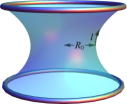
Example: Catenoid. We will examine the behavior of the multipliers on a catenoid bounded by two rings a fixed distance apart. Aligning the axis of symmetry along the $Z$ axis, its radius and height, $R(l)$ and $Z(l)$, can be parameterizing in terms of arc-length $l$ along its meridians (with $l=0$ on the neck of radius $R_{0}$, see Fig. 1(a)): $R(l)=\,\sqrt{1+l^{2}}$, $Z(l)=\mathrm{arcsinh}\,l$, where all lengths are measured in units of $R_{0}$. The principal curvatures along the parallels and meridians are $C_{\parallel}=-C_{\perp}=1/R^{2}$. For simplicity, consider a symmetric section of catenoid bounded by the parallel circles at $l=\pm L$, with corresponding radius $R_{L}$ and height $\pm Z_{L}$ respectively.
By symmetry $\Lambda$ is axially symmetric. Eq. (18) then assumes the form

$$\frac{\left(R\bar{\Lambda}^{\prime}\right)^{\prime}}{R}+2\,\frac{\bar{\Lambda}}{R^{4}}=1\,,$$ (20)

where the prime indicates a derivative with respect to arc-length, and $\bar{\Lambda}:=\Lambda/(4\sigma R_{0}^{2})$. An exact solution of Eq. (20) exists. With the boundary conditions $\Lambda(\pm L)=0$ it is given by

$$\bar{\Lambda}=\frac{l}{4}\left(\frac{1}{R}\ln\left(R+l\right)+l\right)+C_{0}\left(\frac{l}{R}\ln\left(R+l\right)-1\right)\,,$$ (21)

with integration constant,

$$C_{0}=\frac{L}{4}\left(\frac{LR_{L}+\ln(R_{L}+L)}{R_{L}-L\ln(R_{L}+L)}\right)\,.$$ (22)

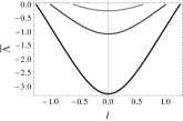
Note that the global minimum, $\Lambda_{0}$, occurs at the neck where the curvature is highest. Furthermore $\bar{\Lambda}_{0}:=\bar{\Lambda}(0)=-C_{0}$ diverges as $L$ is increased to the value $L_{C}=1.50888$ which occurs when $R_{L}=L\ln(R_{L}+L)$ and the ratio of separation $h_{L}=2Z_{L}$ to diameter of the rings $D_{L}=2R_{L}$ is $h_{L}/D_{L}=0.66274$. $\bar{\Lambda}$ is plotted as a function of $l$ for several values of $L$ in the interval $[0,L_{C}]$ in Fig. 1(b). It is negative everywhere in this interval.
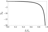
The divergence of $\Lambda_{0}$ at $L=L_{C}$ correlates with the onset of an instability in the catenoid as a minimal surface (see Fig. 1(c)). For let us expand $\Lambda$ in terms of the eigenfunctions of the operator $\mathscr{L}$, $\Lambda=\sum_{n}C_{n}\Phi_{n}$, where $\mathscr{L}\Phi_{n}=E_{n}\Phi_{n}$, so that Eq. (18) reads $\sum_{n}E_{n}C_{n}\Phi_{n}=-4\sigma$. Let $\Phi_{0}$ be the normalized ground state with eigenvalue $E_{0}$. Then

$$E_{0}C_{0}=-4\sigma\int dA\Phi_{0}\,.$$ (23)

If $\Phi_{0}$ is positive everywhere, the left-hand side of Eq. (23) is manifestly negative. If $L$ is small, the catenoid approximates a cylinder with positive $E_{0}$. This implies that $C_{0}$ is negative and thus so also is $\Lambda$, consistent with the exact solution. As $L\to L_{C}$, however, $E_{0}\to 0$. At this value of $L$ Eq. (23) implies that $C_{0}$ must diverge, so that $\Lambda$ does also. Thus an unexpected bonus of this framework is a reformulation of the analysis of stability of minimal surfaces. $L=L_{C}$ is the maximum value of the meridian length for which the catenoid is stable Fomenko . Beyond $L=L_{C}$, $E_{0}$ becomes negative and it can be shown that $\Lambda$ changes sign.

Figure 1: (a) Catenoid between two identic rings. (b) $\Lambda$ as a function of arc-length $l$ for values of boundary arc-length $L=0.6,1,1.25$. The gray scale increases with $L$. (c) Local extrema of the multiplier $\Lambda/(4\sigma R_{0}^{2})$ as a function of the boundary arc-length $L$. (d) $\lambda_{l}$ as a function of arc-length $l$ for the same values of $L$ as in (a).

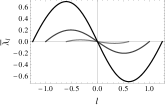
Likewise, defining $\bar{\lambda}_{a}=\lambda_{a}/(4\sigma R_{0}^{2})$, Eqs. (19) are given by

$$\frac{\left(R\bar{\lambda}_{l}^{\prime}\right)^{\prime}}{R}-\frac{\bar{\lambda}_{l}}{R^{4}}=2\frac{\bar{\Lambda}^{\prime}}{R^{2}}\,,\quad\frac{\left(R\bar{\lambda}_{\phi}^{\prime}\right)^{\prime}}{R}-\frac{\bar{\lambda}_{\phi}}{R^{4}}=0\,.$$ (24)

Axial symmetry implies that the angular component vanishes:$\lambda_{\phi}=0$, consistent with the fact that the CM constraint equation along the polar direction vanishes identically: $C_{\phi}=0$. Thus, there is only a generalized force along the meridians. The corresponding component $\lambda_{l}$ is plotted in Fig 1(d) for values of $l$ in the interval $[0,L_{C}]$. It is an antisymmetric function of $l$, possessing two extrema, one maximum and one minimum, vanishing at the neck where $l=0$. Like $\Lambda$, $\lambda_{l}$ diverges at the onset of instability at $L=L_{C}$.

V Conclusions

In this Letter it was shown how a surface can be treated as a Riemannian manifold endowed with a metric that couples to a symmetric tensor field. The GCM equations impose a constraint on these two fields. No direct reference is made to the surface itself.
We have established a framework for studying surfaces that mimics gravity; the surface itself is an emergent entity. In the process, intriguing connections with a theory of metrics are revealed that are likely to be worth exploring.
The metric approach developed here–tweaked appropriately–is ideally adapted to study the recently proposed programmed swelling of thin polymer sheets Hanna . This approach to interfaces and membranes has clear relevance to a number of problems in soft matter: fluctuations or membrane mediated interactions could be treated in a manner that sidesteps the difficulties of the height function representation. Numerically one could contemplate relaxing the GCM equations, but suppress violations in a controlled way by introducing large coupling constants.
One curiosity and unexpected virtue of this framework is that the derivation of the surface Euler-Lagrange equation never requires the explicit determination of the Lagrange multipliers enforcing the constraints. These multipliers are, however, of considerable interest in their own right: it is they that quantify the strength of the coupling between the Riemannian metric and the symmetric tensor field shaping the manifold into a stationary state of the surface. A connection between conformal transformations and surface states has also emerged; its significance remains to be explored. More importantly, however, singularities in the multipliers correlate directly with instabilities in equilibrium surfaces. We have explored in some detail the behavior of these multipliers for surfaces minimizing area and, in particular, a soap film between two rings.
Extending this framework to higher dimensional surfaces or non-trivial backgrounds is not entirely straightforward. Unlike the two-dimensional case examined here, where the contractions of the GCM constraints completely encode their geometrical content, these constraints will need to be accommodated within the Hamiltonian in their full uncontracted glory. In particular, the fortuitous similarity with the ADM formulation of general relativity encountered here becomes an unreliable guidepost; the multiplier fields no longer assemble naturally into a vector field. What is more, the GCM equations will need to be supplemented with their Ricci counterpart if higher codimensions are contemplated Spivak .

Appendix A Making connections and establishing contrasts

It is useful to compare this approach with a variational framework introduced by one of the authors several years ago which adopts a very different strategy auxil . In that approach $H$ is again constructed using the metric and extrinsic curvature as independent variables. In contrast, however, these variables are connected to the embedding functions through the Gauss-Weingarten structure equations. One thus constructs the Hamiltonian

$$H_{C} = H[g_{ab},K_{ab}]$$

$$+ \int dA\,\left[\mathbf{f}^{a}\cdot(\mathbf{e}_{a}-\partial_{a}\mathbf{X})+\lambda_{\perp}^{a}\mathbf{e}_{a}\cdot\mathbf{n}+\lambda_{n}(\mathbf{n}^{2}-1)\right]$$

$$+ \int dA\,\left[\Lambda^{ab}(K_{ab}-\mathbf{e}_{a}\cdot\partial_{b}\mathbf{n})+\,\lambda^{ab}(g_{ab}-\,\mathbf{e}_{a}\cdot\mathbf{e}_{b})\right]\,,$$

implementing the definitions of $g_{ab}$ and $K_{ab}$ in terms of the tangent vectors $\mathbf{e}_{a}$ and the normal $\mathbf{n}$, as well as the connection of the latter to $\mathbf{X}$ by introducing appropriate Lagrange multipliers. One is then free to treat each of these variables independently. In particular, the translational invariance of $H$ implies the existence of a conserved stress tensor. In this framework, $\mathbf{X}$ only appears in the tangential constraint so that

$$\delta_{\bf X}H_{C}=\int dA\nabla_{a}\mathbf{f}^{a}\cdot\delta\mathbf{X}\,,$$ (26)

modulo a boundary term. Thus, in equilibrium, $\nabla_{a}\mathbf{f}^{a}=0$, or the stress $\mathbf{f}^{a}$ is conserved. $\mathbf{f}^{a}$ is constructed using the remaining Euler-Lagrange equations. One finds auxil , $\mathbf{f}^{a}=f^{ab}\mathbf{e}_{b}+f^{a}\mathbf{n}$ , where

$$f^{ab}=T^{ab}-H^{ac}K_{c}{}^{b}\,,\quad f^{a}=-\nabla_{b}H^{ab}\,,$$ (27)

and $T^{ab}$ and $H^{ab}$ were defined in Eq. (7). It depends only on the geometry. In the new framework it is not obvious how to address the Euclidean invariance of the surface Hamiltonian, never mind the conservation laws that it implies, when the surface and its background do not yet exist.
The normal projection of the conservation law reads

$$\nabla_{a}f^{a}-K_{ab}f^{ab}=0\,;$$ (28)

its tangential counterparts $\nabla_{a}f^{ab}+K^{b}_{\phantom{b}a}\,f^{a}=0$, are the statement of reparametrization invariance. Notice that if ${\cal H}$ depends only on $g_{ab}$, Eq. (28) reduces to the statement that $-K_{ab}T^{ab}=0$. This also justifies the strategy that was adopted to identify the surface Euler-Lagrange equation.

References

- (1) D. Nelson, T. Piran y S. Weinberg eds Statistical Mechanics of Membranes and Surfaces vol. 5 (Proceedings of the Jerusalem Winter School for Theoretical Physics) (Singapore: World Scientific 1989)
- (2) S. Hildebrandt and A. Tromba, The Parsimonious Universe: Shape and Form in the Natural World, First edition (Springer, 1996); R. Osserman, A Survey of Minimal Surfaces (Dover Publications, 1986)
- (3) A. M. Polyakov Gauge Fields and Strings (New York: Harwood Academic, 1987)
- (4) M. B. Green, J. H. Schwarz and E. Witten, Superstring Theory, Vol. 1 (Cambridge University Press, 1987); A. Vilenkin and P. Shellard, Cosmic Strings and Other Topological Defects (Cambridge Monographs on Mathematical Physics, 1994).
- (5) M. Spivak, A Comprehensive Introduction to Differential Geometry. Vol.4, Second Edition (Publish or Perish, 1979); M. Do Carmo, Differential geometry of curves and surfaces (Prentice Hall, 1976); Y. Aminov, The Geometry of Submanifolds, First edition (CRC Press, 2001); M. Dajczer, Submanifolds and isometric embeddings (Mathematics Lecture Series, 1990)
- (6) J. Eells and J. H. Sampson, Am. J. Math. 86, 109 (1964).
- (7) J. Guven J. Phys. A: Math and Gen. 37 L313 (2004).
- (8) J. Barbour, B. Foster and N. Ó Murchadha, Class. Quant. Grav. 19 3217-3248 (2002);
- (9) R. Sorkin, Modern Physics Letters A 17, 695 (2002)
- (10) M. A. Lomholt and L. Miao, J. Phys. A: Math. Gen. 39 10323 (2006)
- (11) J. Guven and M. M. Müller, J. Phys. A: Math and Theor. 41 055203 (2008)
- (12) C. W. Misner, K. S. Thorne and J. A. Wheeler, Gravitation, First Edition edition (W. H. Freeman, Physics Series, 1973); S. M. Carroll, Spacetime and Geometry: An Introduction to General Relativity (Addison-Wesley, 2003).
- (13) R. Capovilla and J. Guven, Phys Rev. D 51 (12), 6736 (1995); R. Capovilla and J. Guven, J. Phys. A: Math. and Gen. 35 6233 (2002).
- (14) R. Arnowitt, S. Deser, and C. W. Misner, Phys. Rev. 116, 1322 (1959); M. Alcubierre, Introduction to 3+1 Numerical Relativity (Oxford University Press, International Series of Monographs on Physics, 2008)
- (15) T. J. Willmore, Total Curvature in Riemannian Geometry (Chichester: Ellis Horwood, 1982).
- (16) P. Canham, J. Theor. Biol. 26 61 (1970); W. Helfrich, Z. Naturf. C 28 693 (1973); for a review see U. Seifert, Adv. in Phys. 46 13. (1997).
- (17) J. Guven, D.M. Valencia and P. Vázquez-Montejo In preparation
- (18) A. T. Fomenko and A. A. Tuzhilin, Elements of the Geometry and Topology of Minimal Surfaces in Three-Dimensional Space (American Mathematical Society, Translations of Mathematical Monographs, 93, 2005)
- (19) M.A. Dias, J.A. Hanna and C.D. Santangelo, Phys. Rev. E 84, 036603 (2011)