Domain decomposition methods for problems of unilateral contact between elastic bodies with nonlinear Winkler covers

Abstract

In this paper we propose on continuous level a class of domain decomposition methods of Robin–Robin type to solve the problems of unilateral contact between elastic bodies with nonlinear Winkler covers. These methods are based on abstract nonstationary iterative algorithms for nonlinear variational equations in reflexive Banach spaces. We also provide numerical investigations of obtained methods using finite element approximations.

Key words: unilateral contact, nonlinear Winkler layers, nonlinear variational inequalities, nonlinear variational equations, iterative methods, domain decomposition

MSC2010: 65N55, 74S05

1 Introduction

Thin covers from another material are often applied in engineering to improve the functional properties of the surfaces of components of machines and structures. On the other hand, thin covers with certain mechanical properties are used for modeling of real microstructure of the surfaces, adhesion and glue bondings [6, 14, 15].

The classical methods for solution of contact problems for bodies with thin covers are grounded on integral equations and are reviewed in work [15]. Nowadays, one of the most effective numerical methods for such contact problems are methods, based on variational formulations and finite element approximations.

Efficient approach for solution of multibody contact problems is the use of domain decomposition methods (DDMs). Many DDMs for contact problems without covers are obtained on discrete level [3, 16]. Among DDMs, proposed on continuous level for contact problems without covers are methods presented in [1, 9, 12]. Domain decomposition methods for solution of problem of ideal contact between two bodies, connected through nonlinear Winkler layer are proposed in [2, 8]. These methods are based on saddle-point formulation and conjugate gradient methods.

In current contribution we consider the problem of unilateral contact between bodies with nonlinear Winkler covers. We give variational formulations of this problem in the form of nonlinear variational inequality on convex set and variational equation in the whole space, and present theorems about existence and uniqueness of their solution. Furthermore, we propose on continuous level a class of parallel domain decomposition methods for solving the nonlinear variational equation, which corresponds to original contact problem. In each iteration of these methods we have to solve in a parallel way linear variational equations in separate bodies, which are equivalent in a weak sense to linear elasticity problems with Robin boundary conditions on possible contact areas. These DDMs are based on abstract nonstationary iterative methods for variational equations in Banach spaces. They are the generalization of domain decomposition methods, proposed by us earlier in [4, 5, 10] for unilateral contact problems without covers. Some particular cases of proposed DDMs can be viewed as a modification of semismooth Newton method [7]. The numerical analysis of obtained DDMs is made for plane contact problems using finite element approximations.

2 Statement of the problem

Consider a unilateral contact of $N$ elastic bodies $\Omega_{\alpha}\subset{\mathbb{R}}^{3}$ with piecewise smooth boundaries $\Gamma_{\alpha}$, $\alpha=1,2,...,N$ (Fig. 1a). Suppose that across each contact surface there is a nonlinear Winkler layer. Denote $\Omega=\bigcup_{\alpha=1}^{N}\Omega_{\alpha}$.

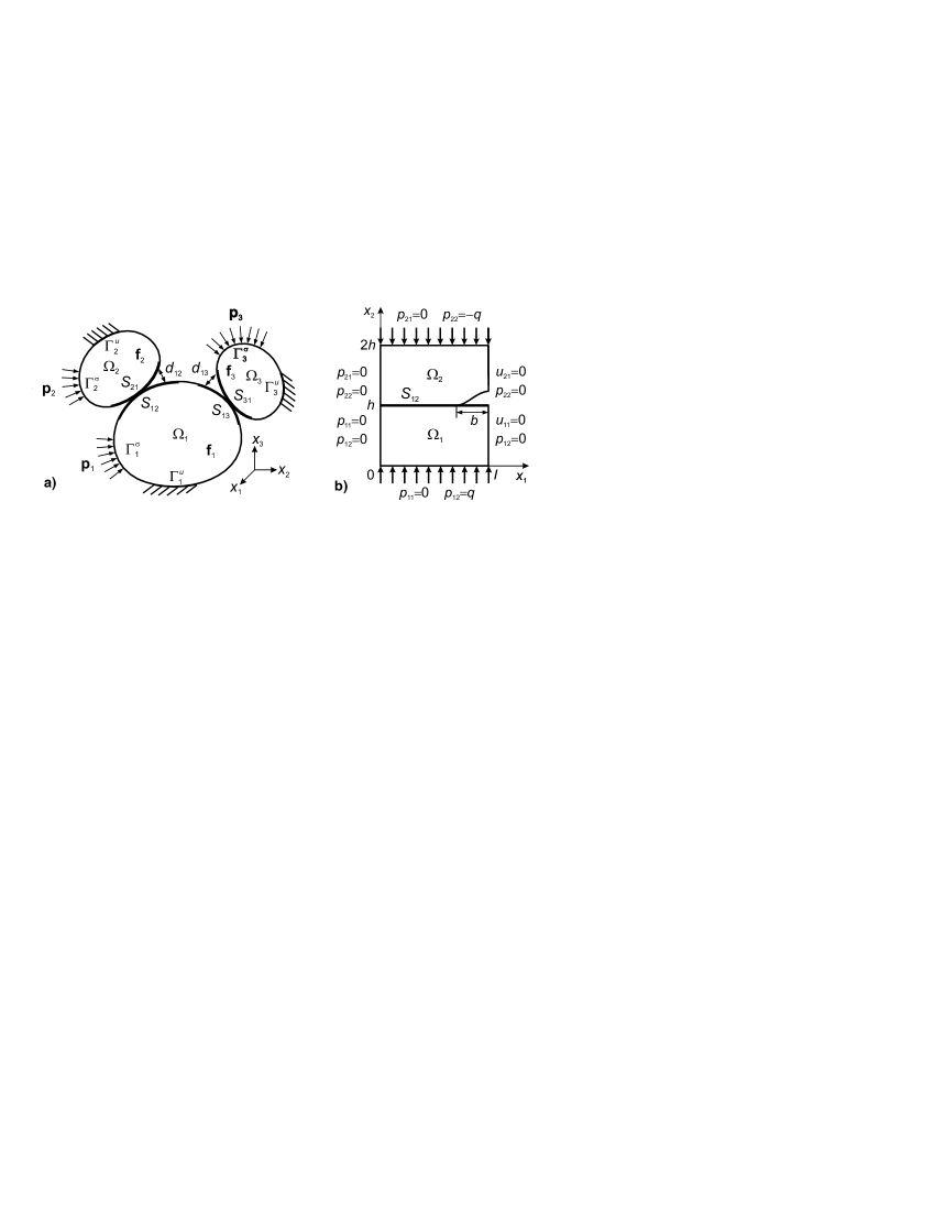
Figure 1: Unilateral contact between several elastic bodies through nonlinear Winkler layers

A stress-strain state in point ${\bf x}=(x_{1},x_{2},x_{3})^{\top}$ of each solid $\Omega_{\alpha}$ is described by the displacement vector ${\bf u}_{\,\alpha}=u_{\alpha\,i}\,{\bf e}_{i}\,$, the tensor of strains ${\hat{\boldsymbol{\varepsilon}}}_{\alpha}=\varepsilon_{\alpha\,ij}\,{\bf e}_{i}\,{\bf e}_{j}$ and the tensor of stresses $\hat{{\boldsymbol{\sigma}}}_{\alpha}=\sigma_{\alpha\,ij}\,{\bf e}_{i}\,{\bf e}_{j}$. These quantities satisfy the following relations:

$$\sum_{j=1}^{3}\frac{\partial\sigma_{\alpha\,ij}({\bf x})}{\partial x_{j}}\,+f_{\alpha\,i}({\bf x})=0\,,\,\,\,\,{\bf x}\in{\Omega}_{\alpha}\,,\,\,\,\,i=1,2,3\,,$$ (1)

$$\sigma_{\alpha\,ij}({\bf x})=\sum_{k,l=1}^{3}C_{\alpha\,ijkl}({\bf x})\,\varepsilon_{\alpha\,kl}({\bf x})\,,\,\,\,\,{\bf x}\in{\Omega}_{\alpha}\,,\,\,\,\,i,j=1,2,3\,,$$ (2)

$$\varepsilon_{\alpha\,ij}({\bf x})=\frac{1}{2}\left(\frac{\partial u_{\alpha\,i}({\bf x})}{\partial x_{j}}+\frac{\partial u_{\alpha\,j}({\bf x})}{\partial x_{i}}\right)\,,\,\,\,\,{\bf x}\in{\Omega}_{\alpha},\,\,\,\,i,j=1,2,3\,,$$ (3)

where $f_{\alpha\,i}$ are the components of volume forces vector ${\,\bf f}_{\alpha}=f_{\alpha\,i}\,{\bf e}_{i}$, and $C_{\alpha\,ijkl}$ are symmetric elasticity constants, which are bounded in the following sense:

$$\left(\exists b_{\alpha},c_{\alpha}>0\right)\left(\forall{\bf x}\right)\left\{b_{\alpha}\sum_{i,j=1}^{3}\varepsilon_{\alpha ij}^{2}\leq\sum_{i,j,k,l=1}^{3}C_{\alpha ijkl}\varepsilon_{\alpha ij}\varepsilon_{\alpha kl}\leq c_{\alpha}\sum_{k,l=1}^{3}\varepsilon_{\alpha kl}^{2}\right\}.$$ (4)

Introduce on boundary $\Gamma_{\alpha}$ a local orthonormal coordinate system ${\boldsymbol{\xi}}_{\alpha},\,{\boldsymbol{\eta}}_{\alpha},\,{\bf n}_{\alpha}$, where ${\bf n}_{\alpha}$ is an outer unit normal. Then the vectors of displacements and stresses on $\Gamma_{\alpha}$ can be written in the following way: ${\bf u}_{\,\alpha}=u_{\alpha\,\xi}\,{\boldsymbol{\xi}}_{\alpha}+u_{\alpha\eta}\,{\boldsymbol{\eta}}_{\alpha}+u_{\alpha n}\,\bf{n}_{\,\alpha},\,\,{\boldsymbol{\sigma}}_{\alpha}=\hat{{\boldsymbol{\sigma}}}_{\alpha}\cdot n_{\,\alpha}=\sigma_{\alpha\xi}\,{\boldsymbol{\xi}}_{\alpha}+\sigma_{\alpha\eta}\,{\boldsymbol{\eta}}_{\alpha}+\sigma_{\alpha\it n}\,n_{\,\alpha}\,.$

Suppose, that the boundary $\Gamma_{\alpha}$ consists of three disjoint parts:
$\Gamma_{\alpha}=\Gamma_{\alpha}^{u}\bigcup\Gamma_{\alpha}^{\sigma}\bigcup S_{\alpha}$, $\Gamma_{\alpha}^{u}=\overline{\Gamma_{\alpha}^{u}}$, $\Gamma_{\alpha}^{u}\neq\emptyset$, $S_{\alpha}\neq\emptyset$. On the part $\Gamma_{\alpha}^{u}$ homogenous Dirichlet boundary conditions are prescribed, and on the part $\Gamma_{\alpha}^{\sigma}$ we consider Neumann boundary conditions:

$${\bf u}_{\,\alpha}({\bf x})=0,\,\,\,{\bf x}\in\Gamma_{\alpha}^{u}\,;\,\,\,\,\,{\boldsymbol{\sigma}}_{\alpha}({\bf x})={\bf p}_{\alpha}({\bf x}),\,\,\,{\bf x}\in\Gamma_{\alpha}^{\sigma}\,.$$ (5)

The part $S_{\alpha}=\bigcup_{\beta\in B_{\alpha}}S_{\alpha\beta}$, $\bigcap_{\beta\in B_{\alpha}}S_{\alpha\beta}=\emptyset$ is the possible contact area of body $\Omega_{\alpha}$ with the other bodies. Here $S_{\alpha\beta}$ is the possible unilateral contact area of body $\Omega_{\alpha}$ with body $\Omega_{\beta}$, and $B_{\alpha}\subset\left\{1,2,...,N\right\}$ is the set of the indices of all bodies in contact with body $\Omega_{\alpha}$. We assume that the surfaces $S_{\alpha\beta}\subset\Gamma_{\alpha}$ and $S_{\beta\alpha}\subset\Gamma_{\beta}$ are sufficiently close ($S_{\alpha\beta}\approx S_{\beta\alpha}$), and ${\bf n}_{\,\alpha}({\bf x})\approx-{\bf n}_{\,\beta}({\bf x}^{\prime})$, ${\bf x}\in S_{\alpha\beta}$, ${\bf x}^{\prime}=P({\bf x})\in S_{\beta\alpha}$, where $P({\bf x})$ is the projection of point ${\bf x}$ on $S_{\alpha\beta}$. Let $d_{\,\alpha\beta}({\bf x})=\pm\left\|{\bf x}-{\bf x}^{\prime}\right\|=\pm\sqrt{\sum_{i=1}^{3}\left(x_{i}-x^{\prime}_{i}\right)^{2}}$ be a distance between bodies $\Omega_{\alpha}$ and $\Omega_{\beta}$ before the deformation.

We suppose that possible contact areas $S_{\alpha\beta}$ and $S_{\beta\alpha}$, $\beta\in B_{\alpha}$, $\alpha=1,...,N$  have nonlinear Winkler covers. Total compression $w_{\alpha\beta}$ of these covers is related with normal contact stress as follows: $\sigma_{\alpha n}({\bf x})=\sigma_{\beta n}({\bf x}^{\prime})=g_{\alpha\beta}\left(w_{\alpha\beta}({\bf x})\right)$, ${\bf x}\in S_{\alpha\beta}$, ${\bf x}^{\prime}\in S_{\beta\alpha}$, where $g_{\alpha\beta}$ is given nonlinear continuous function, which satisfy the next conditions:

$$g_{\alpha\beta}(0)=0\,,\,\,\,\,\,\left(\forall\,y,z\right)\,\left\{\,y<z\,\Rightarrow g_{\alpha\beta}(y)<g_{\alpha\beta}(z)\,\right\},$$ (6)

$$\left(\exists\,M_{\alpha\beta}>0\right)\,\left(\forall\,y,z\right)\,\left\{\,\left|g_{\alpha\beta}(y)-g_{\alpha\beta}(z)\right|\leq M_{\alpha\beta}\left|y-z\right|\,\right\}.$$ (7)

On possible contact zones $S_{\alpha\beta}$, $\beta\in B_{\alpha}$, $\alpha=1,2,...,N$ we consider the following unilateral contact conditions through nonlinear Winkler layers:

$$\sigma_{\alpha\xi}({\bf x})=\sigma_{\beta\xi}({\bf x}^{\prime})=0\,,\,\,\,\,\sigma_{\alpha\eta}({\bf x})=\sigma_{\beta\eta}({\bf x}^{\prime})=0\,,$$ (8)

$$\sigma_{\alpha n}({\bf x})=\sigma_{\beta n}({\bf x}^{\prime})=g_{\alpha\beta}\left(w_{\alpha\beta}({\bf x})\right)\leq 0\,,$$ (9)

$$u_{\alpha n}({\bf x})+u_{\beta n}({\bf x}^{\prime})+w_{\alpha\beta}({\bf x})\leq d_{\,\alpha\beta}({\bf x})\,,$$ (10)

$$\left[\,u_{\alpha n}({\bf x})+u_{\beta n}({\bf x}^{\prime})+w_{\alpha\beta}({\bf x})-d_{\alpha\beta}({\bf x})\,\right]\sigma_{\alpha n}({\bf x})=0,\,{\bf x}^{\prime}=P({\bf x}),\,{\bf x}\in S_{\alpha\beta}.$$ (11)

3 Variational formulations

For each body $\Omega_{\alpha}$ consider Sobolev space $V_{\alpha}=[H^{1}(\Omega_{\alpha})]^{3}$ and the closed subspace $V_{\alpha}^{0}=\left\{{\bf u}_{\,\alpha}\in V_{\alpha}:\,\,{\bf u}_{\,\alpha}=0\,\,\,{\rm on}\,\,\Gamma_{\alpha}^{u}\right\}$. All values of the elements from these spaces on the parts of boundary $\Gamma_{\alpha}$ should be understood as traces. The trace of element ${\bf u}_{\alpha}\in V_{\alpha}$ on the part $\Gamma_{\alpha}^{u}$ should belong to space $[H^{1/2}(\Gamma_{\alpha}^{u})]^{3}$, and the trace of element from $V_{\alpha}^{0}$ on the part $\Xi_{\alpha}=\textrm{int}\,(\Gamma_{\alpha}\setminus\Gamma_{\alpha}^{u})$ should belong to $[H_{00}^{1/2}(\Xi_{\alpha})]^{3}$.

Define Hilbert space $V_{0}=\prod_{\alpha=1}^{N}V_{\alpha}$ with scalar product
$\left({\bf u}\,,{\bf v}\right)_{V_{0}}=\sum_{\alpha=1}^{N}\left({\bf u}_{\,\alpha},{\bf v}_{\alpha}\right)_{V_{\alpha}}$ and norm $\left\|{\bf u}\right\|_{V_{0}}=\left({\bf u}\,,{\bf u}\right)_{V_{0}}^{1/2}$, ${\bf u},{\bf v}\in V_{0}$. Moreover, introduce following spaces $W=\prod_{\{\alpha,\,\beta\}\in Q}H_{00}^{1/2}({\Xi}_{\alpha})=\{{\bf w}=(w_{\alpha\beta})_{\{\alpha,\,\beta\}\in Q}^{\top}:\,\,\,w_{\alpha\beta}\in H_{00}^{1/2}\}$ and $U_{0}=V_{0}\times W=\{{\bf U}=({\bf u},{\bf w})^{\top}:\,\,\,{\bf u}\in V_{0},\,{\bf w}\in W\}$, where $Q=\left\{\left\{\alpha,\beta\right\}:\,\,\alpha\in\left\{1,2,...,N\right\},\,\,\beta\in B_{\alpha}\right\}$.

In space $U_{0}$ consider the closed convex set of all displacements, which satisfy nonpenentration contact conditions:

$$K=\{{\bf U}\in U_{0}:\,\,\,u_{\alpha n}+u_{\beta n}+w_{\alpha\beta}\leq d_{\alpha\beta}\,\,\,{\rm on}\,\,\,S_{\alpha\beta},\,\,\,\{\alpha,\,\beta\}\in Q\,\},$$ (12)

where $u_{\alpha\,n}={\bf n}_{\alpha}\cdot{\bf u}_{\alpha}\in H_{00}^{1/2}(\Xi_{\alpha})$, $w_{\alpha\beta},d_{\alpha\beta}\in H_{00}^{1/2}(\Xi_{\alpha})$.

Let us introduce bilinear form $A({\bf u},{\bf v})$, such that $A({\bf u},{\bf u})$ represents the total elastic deformation energy of the bodies, linear form $L({\bf u})$, which is equal to external forces work, and nonquadratic functional $H({\bf w})$, which represents the total deformation energy of nonlinear Winkler layers:

$$A\,({\bf u},{\bf v})=\sum_{\alpha=1}^{N}a_{\alpha}({\bf u}_{\,\alpha},{\bf v}_{\alpha}),\,\,\,\,a_{\alpha}({\bf u}_{\alpha},{\bf v}_{\alpha})=\int_{\Omega_{\,\alpha}}\hat{\boldsymbol{\sigma}}_{\alpha}({\bf u}_{\alpha})\,\,:\hat{\boldsymbol{\varepsilon}}_{\alpha}({\bf v}_{\alpha})\,d\Omega\,,$$ (13)

$$L\,({\bf u})=\sum_{\alpha=1}^{N}l_{\alpha}({\bf u}_{\,\alpha}),\,\,\,\,l_{\alpha}({\bf u}_{\alpha})=\int_{\Omega_{\alpha}}{\bf f}_{\,\alpha}\cdot{\bf u}_{\alpha}\,d\Omega+\int_{\Gamma_{\alpha}^{\,\sigma}}{\bf p}_{\alpha}\cdot{\bf u}_{\alpha}\,dS\,\,,$$ (14)

$$H({\bf w})=\sum_{\{\alpha,\,\beta\}\in Q}\int_{S_{\alpha\beta}}\left[\int_{0}^{w_{\alpha\beta}}g_{\alpha\beta}(z)\,dz\right]dS\,,\,\,\,\,{\bf u},{\bf v}\in V_{0}\,,\,\,\,\,{\bf w}\in W\,,$$ (15)

where ${\bf f}_{\,\alpha}\in[L_{2}(\Omega_{\alpha})]^{3}$, ${\bf p}_{\alpha}\in[H_{00}^{-1/2}(\Xi_{\alpha})]^{3}$, $\alpha=1,2,...,N$.

We have shown, that if condition (4) holds then bilinear form $A$ is symmetric, continuous and coercive, and nonquadratic functional $H$ is Gateaux differentiable:

$$H^{\prime}({\bf w},{\bf z})=\sum_{\{\alpha,\,\beta\}\in Q}\int_{S_{\alpha\beta}}g_{\alpha\beta}(w_{\alpha\beta})\,z_{\alpha\beta}\,dS\,,\,\,\,\,{\bf w},{\bf z}\in W\,.$$ (16)

Theorem 1. Suppose that conditions (4), (6), (7) hold. Then problem (1)–(3), (5), (8)–(11) has an alternative weak formulation as the following minimization problem:

$$F({\bf U})=A\,({\bf u},{\bf u})/2-L\,({\bf u})+H({\bf w})\to\mathop{\min}\limits_{{\bf U}\,\in\,K}.$$ (17)

Moreover, there exists a unique solution of problem (17), and this problem is equivalent to the following nonlinear variational inequality on set $K$:

$$F^{\prime}({\bf U},{\bf V}-{\bf U})=A\,({\bf u},{\bf v}-{\bf u})-L\,({\bf v}-{\bf u})+H^{\prime}({\bf w},{\bf z}-{\bf w})\geq 0\,,\,\,\,\,\forall\,({\bf v},{\bf z})^{\top}\in K\,.$$ (18)

Except this variational formulation, we also have proposed another weak formulation of original contact problem in the form of nonlinear variational equation.

Let us introduce the following nonquadratic functional in space $V_{0}$:

$$J({\bf u})=\sum_{\{\alpha,\,\beta\}\in Q}\int_{S_{\alpha\beta}}\left[\int_{0}^{d_{\alpha\beta}-u_{\alpha n}-u_{\beta n}}g_{\alpha\beta}^{-}(z)\,dz\right]dS\,,\,\,\,\,{\bf u}\in V_{0}\,,$$ (19)

where $g_{\alpha\beta}^{-}(z)=\{\,0\,,\,\,z\geq 0\,\}\vee\{\,g_{\alpha\beta}(z)\,,\,\,z<0\,\}$ is nonlinear function.

Functional $J({\bf u})$ is nonnegative and Gateaux differentiable in $V_{0}$:

$$J^{\prime}({\bf u},{\bf v})=-\sum_{\{\alpha,\,\beta\}\in Q}\int_{S_{\alpha\beta}}g_{\alpha\beta}^{-}(d_{\alpha\beta}-u_{\alpha n}-u_{\beta n})\,\,[v_{\alpha n}+v_{\beta n}]\,dS\,.$$ (20)

We have shown that if conditions (6) and (7) hold, then Gateaux differential $J^{\prime}({\bf u},{\bf v})$ satisfies the following properties:

$$(\forall\,{\bf u}\in V_{0})\,\,(\exists\,\tilde{R}>0\,)\,\,(\forall\,{\bf v}\in V_{0})\,\left\{\,\left|J^{\prime}({\bf u},{\bf v})\right|\leq\tilde{R}\left\|{\bf v}\right\|_{V_{0}}\right\},$$ (21)

$$(\exists\,\tilde{D}>0)\,(\forall\,{\bf u},{\bf v},{\bf w}\!\in\!V_{0})\!\,\left\{\!\,\left|J^{\prime}({\bf u}+{\bf w},{\bf v})\!-\!J^{\prime}({\bf u},{\bf v})\,\!\right|\!\leq\!\tilde{D}\left\|{\bf v}\right\|_{V_{0}}\!\left\|{\bf w}\right\|_{V_{0}}\!\,\right\},$$ (22)

$$\left(\forall\,{\bf u},{\bf v}\in V_{0}\right)\,\left\{\,J^{\prime}({\bf u}+{\bf v},{\bf v})-J^{\prime}({\bf u},{\bf v})\geq 0\,\right\}.$$ (23)

These properties helped us to prove the next theorem.

Theorem 2. Suppose that conditions (4), (6) and (7) hold. Then the contact problem (1)–(3), (5), (8)–(11) is equivalent to problem (1)–(3), (5), (8) with the following nonlinear boundary value conditions on the possible contact areas:

$$\sigma_{\alpha n}({\bf x})=\sigma_{\beta n}({\bf x}^{\prime})=g_{\alpha\beta}^{-}\left(d_{\alpha\beta}({\bf x})-u_{\alpha n}({\bf x})-u_{\beta n}({\bf x}^{\prime})\right)\,,\,\,\,{\bf x}^{\prime}=P({\bf x})\,,\,\,\,{\bf x}\in S_{\alpha\beta}\,,$$ (24)

and it is equivalent in weak sense to the next nonquadratic minimization problem:

$$F_{1}({\bf u})=A\,({\bf u},{\bf u})/2-L\,({\bf u})+J({\bf u})\to\mathop{\min}\limits_{{\bf u}\,\in\,V_{0}}.$$ (25)

Moreover, problem (25) has a unique solution and is equivalent to the next nonlinear variational equation in space $V_{0}$:

$$F^{\prime}_{1}({\bf u},{\bf v})=A\,({\bf u},{\bf v})+J^{\prime}({\bf u},{\bf v})-L\,({\bf v})=0,\,\,\,\,\forall\,{\bf v}\in V_{0}\,,\,\,\,{\bf u}\in V_{0}\,.$$ (26)

4 Nonstationary iterative methods

In reflexive Banach space $V$ consider an abstract nonlinear variational equation

$$\Phi\,({\bf u},{\bf v})=Y({\bf v})\,,\,\,\,\,\forall\,{\bf v}\in V,\,\,\,\,{\bf u}\in V,$$ (27)

where $\Phi:\,\,V\times V\to{\mathbb{R}}$ is a functional, which is linear in ${\bf v}$, but nonlinear in ${\bf u}$, and $Y:\,\,V\to{\mathbb{R}}$ is linear continuous form. For numerical solution of (27) consider the next nonstationary iterative method [5, 11]:

$$G^{k}({\bf u}^{k+1},{\bf v})=G^{k}({\bf u}^{k},{\bf v})-\gamma^{k}\left[\,\Phi\,({\bf u}^{k},{\bf v})-Y({\bf v})\,\right],\,\,\,\,k=0,1,...\,\,,$$ (28)

where $G^{k}:\,\,V\times V\to{\mathbb{R}}$ are some given bilinear forms, ${\gamma}^{k}\in{\mathbb{R}}$ are iterative parameters, and ${\bf u}^{k}\in V$ is the k-th approximation to the exact solution of problem (27).

Theorem 3. [5]  Suppose that functional $\Phi$ satisfies the following properties:

$$\left(\forall{\bf u}\in V\right)\left(\exists R_{\Phi}>0\,\right)\left(\forall{\bf v}\in V\right)\left\{\,\left|\Phi\,({\bf u},{\bf v})\right|\leq R_{\Phi}\left\|{\bf v}\right\|_{V}\right\},$$ (29)

$$\left(\exists D_{\Phi}\!>\!0\right)\!\,\left(\forall{\bf u},{\bf v},{\bf w}\!\in\!V\right)\!\,\left\{\,\!\,\left|\Phi\,({\bf u}+{\bf w},{\bf v})-\Phi\,({\bf u},{\bf v})\,\!\right|\leq D_{\Phi}\!\left\|{\bf v}\right\|_{V}\!\left\|{\bf w}\right\|_{V}\!\,\right\},$$ (30)

$$\left(\exists B_{\Phi}>0\right)\left(\forall{\bf u},{\bf v}\in V\right)\,\left\{\,\Phi\,({\bf u}+{\bf v},{\bf v})-\Phi\,({\bf u},{\bf v})\geq B_{\Phi}\left\|{\bf v}\right\|_{V}^{2}\right\}.$$ (31)

Then nonlinear variational equation (27) has a unique solution $\bar{{\bf u}}\in V$. In addition, suppose that bilinear forms $G^{k}$, $k=0,1,...$ are symmetric, continuous with constant $M_{G}^{*}>0$, coercive with constant $B_{G}^{*}>0$, and the next conditions hold:

$$\left(\exists k_{0}\in{\mathbb{N}}_{0}\right)\left(\forall k\geq k_{0}\right)\,\left(\forall{\bf u}\in V\right)\,\left\{\,G^{k}({\bf u},{\bf u})\geq G^{k+1}({\bf u},{\bf u})\right\},$$ (32)

$$\left(\exists\varepsilon\in(0,\,\gamma^{*}),\,\,\gamma^{*}={B_{\Phi}B_{G}^{*}\mathord{\left/{\vphantom{B_{\Phi}B_{G}^{*}D_{\Phi}^{2}}}\right.\kern-1.2pt}D_{\Phi}^{2}}\right)\left(\exists k_{1}\right)\left(\forall k\geq k_{1}\right)\,\left\{\,\gamma^{k}\in[\varepsilon,\,2\gamma^{*}-\varepsilon]\,\right\},$$ (33)

where $\{{\bf u}^{k}\}\subset V$ is obtained by iterative method (28).

5 Domain decomposition schemes

Now let us apply nonstationary iterative method (28) for solving nonlinear variational equation (26), which corresponds to original contact problem. This equation can be written in form (27), where $\Phi({\bf u},{\bf v})=A\,({\bf u},{\bf v})+J^{\prime}({\bf u},{\bf v})\,$, $Y({\bf v})=L\,({\bf v})\,$, ${\bf u},{\bf v}\in V$, $V=V_{0}\,$, and iterative method (28) applied to solve (26) rewrites as follows:

$$G^{k}({\bf u}^{k+1},{\bf v})=G^{k}({\bf u}^{k},{\bf v})-\gamma^{k}\left[A\,({\bf u}^{k},{\bf v})+J^{\prime}({\bf u}^{k},{\bf v})-L({\bf v})\right],\,k=0,1,....$$ (34)

Note, that in general case iterative method (34) does not lead to domain decomposition. Let us propose such variants of this method, which involve the domain decomposition. At first, let us take bilinear forms $G^{k}$ in method (34) as follows:

$$G^{k}({\bf u},{\bf v})=\partial^{2}F_{1}({\bf u}^{k},{\bf u},{\bf v})=A\,({\bf u},{\bf v})+\partial^{2}J({\bf u}^{k},{\bf u},{\bf v})\,,\,\,\,\,{\bf u},{\bf v}\in V_{0}\,,$$ (35)

$$\partial^{2}J({\bf u}^{k},{\bf u},{\bf v})=\sum_{\{\alpha,\,\beta\}\in Q}\int_{S_{\alpha\beta}}\chi_{\alpha\beta}^{k}\,g^{\prime}_{\alpha\beta}(d_{\alpha\beta}-u_{\alpha n}^{k}-u_{\beta n}^{k})\left[u_{\alpha n}+u_{\beta n}\right]\left[v_{\alpha n}+v_{\beta n}\right]dS,$$

$${\chi}_{\alpha\beta}^{k}=-[\,\textrm{sgn}\,(d_{\alpha\beta}-u_{\alpha n}^{k}-u_{\beta n}^{k})\,]^{-}=\{\,0,\,d_{\alpha\beta}-u_{\alpha n}^{k}-u_{\beta n}^{k}\geq 0\,\}\vee\{\,1,\,\textrm{else}\,\}.$$ (36)

Here $\partial^{2}F_{1}({\bf u}^{k},{\bf u},{\bf v})$ and $\partial^{2}J({\bf u}^{k},{\bf u},{\bf v})$ are the second subdifferentials of functionals $F_{1}$ and $J$ in point ${\bf u}^{k}\in V_{0}$. In the case when ${\gamma}^{k}=1$, $k=0,1,...\,$, iterative method (34) with bilinear forms (35) corresponds to semismooth Newton method for variational equation (26). However, this method does not lead to domain decomposition.

Now, let us take bilinear forms $G^{k}$ in the following way:

$$G^{k}({\bf u},{\bf v})=A\,({\bf u},{\bf v})+X^{k}({\bf u},{\bf v})\,,\,\,\,\,{\bf u},{\bf v}\in V_{0}\,,$$ (37)

$$X^{k}({\bf u},{\bf v})=\sum_{\alpha=1}^{N}\sum_{\,\beta\in B_{\alpha}}\int_{S_{\alpha\beta}}\psi_{\alpha\beta}^{k}\,g^{\prime}_{\alpha\beta}(d_{\alpha\beta}-u_{\alpha n}^{k}-u_{\beta n}^{k})\,u_{\alpha n}v_{\alpha n}dS,\,\,{\bf u},{\bf v}\in V_{0},$$ (38)

where $\psi_{\alpha\beta}^{k}({\bf x})=\{\,1,\,{\bf x}\in S_{\alpha\beta}^{k}\,\}\vee\{\,0,\,{\bf x}\in S_{\alpha\beta}\backslash S_{\alpha\beta}^{k}\,\}$ are characteristic functions of some given subsets $S_{\alpha\beta}^{k}\subseteq S_{\alpha\beta}$ of possible contact areas.

Let us show, that such choice of bilinear forms $G^{k}$ involves the domain decomposition. Introduce a notation $\tilde{{\bf u}}^{k+1}=({\bf u}^{k+1}-{\bf u}^{k})/{\gamma}^{k}+{\bf u}^{k}\in V_{0}$. Then iterative method (34) with bilinear forms (37) can be written in such way:

$$A\,(\tilde{{\bf u}}^{k+1},{\bf v})+X^{k}(\tilde{{\bf u}}^{k+1},{\bf v})=L\,({\bf v})+X^{k}({\bf u}^{k},{\bf v})-J^{\prime}({\bf u}^{k},{\bf v})\,,\,\,\,\forall\,{\bf v}\in V_{0}\,.$$ (39)

$${\bf u}^{k+1}={\gamma}^{k}\,\tilde{{\bf u}}^{k+1}+(1-{\gamma}^{k})\,{\bf u}^{k},\,\,\,\,k=0,1,...\,.$$ (40)

Since the common quantities of the subdomains are known from the previous iteration, variational equation (39) splits into $N$ separate equations in subdomains $\Omega_{\alpha}\,$, and iterative method (39)–(40) can be written in the following equivalent form:

$$a_{\alpha}(\tilde{{\bf u}}_{\alpha}^{k+1},{\bf v}_{\alpha})+\sum_{\beta\,\in B_{\alpha}}\int_{S_{\alpha\beta}}\psi_{\alpha\beta}^{k}\,g^{\prime}_{\alpha\beta}(d_{\alpha\beta}-u_{\alpha n}^{k}-u_{\beta n}^{k})\,\tilde{u}_{\alpha n}^{k+1}v_{\alpha n}\,dS=$$

$$=l_{\alpha}({\bf v}_{\alpha})+\sum_{\beta\,\in B_{\alpha}}\int_{S_{\alpha\beta}}\psi_{\alpha\beta}^{k}\,g^{\prime}_{\alpha\beta}(d_{\alpha\beta}-u_{\alpha n}^{k}-u_{\beta n}^{k})\,u_{\alpha n}^{k}v_{\alpha n}\,dS\,+$$

$$+\sum_{\beta\,\in B_{\alpha}}\int_{S_{\alpha\beta}}g_{\alpha\beta}^{-}(d_{\alpha\beta}-u_{\alpha n}^{k}-u_{\beta n}^{k})\,v_{\alpha n}\,dS\,,\,\,\,\,\forall\,{\bf v}_{\alpha}\in V_{\alpha}^{0}\,,$$ (41)

$${\bf u}_{\alpha}^{k+1}={\gamma}^{k}\,\tilde{{\bf u}}_{\alpha}^{k+1}+(1-{\gamma}^{k})\,{\bf u}_{\alpha}^{k}\,,\,\,\,\,\alpha=1,2,...,N,\,\,\,\,k=0,1,...\,.$$ (42)

In each iteration $k$ of method (41)–(42), we have to solve $N$ linear variational equations (41) in parallel, which correspond to linear elasticity problems in separate bodies $\Omega_{\alpha}$ with Robin boundary conditions on possible contact areas. Therefore, this method refers to parallel Robin–Robin type domain decomposition schemes.

By taking different characteristic functions $\psi_{\alpha\beta}^{k}$, we can obtain different particular cases of domain decomposition method (41)–(42). Thus, taking $\psi_{\alpha\beta}^{k}({\bf x})\equiv 0$ $(S_{\alpha\beta}^{k}=\emptyset)$, $\forall\alpha,\beta$, $\forall k$, we get parallel Neumann–Neumann domain decomposition scheme. Other borderline case is when $\psi_{\alpha\beta}^{k}({\bf x})\equiv 1$ $(S_{\alpha\beta}^{k}=S_{\alpha\beta})$, $\forall\alpha,\beta$, $\forall k$.

Moreover, we can choose characteristic functions $\psi_{\alpha\beta}^{k}$ by formula (36), i.e. $\psi_{\alpha\beta}^{k}=\chi_{\alpha\beta}^{k}$. Numerical experiments, provided by us, have shown, that such DDM has higher convergence rate than other particular domain decomposition schemes.

6 Numerical investigations

Numerical investigations of proposed DDMs have been made for plane problem of unilateral contact between two isotropic bodies ${\Omega}_{1}$ and ${\Omega}_{2}$, one of which has a groove (Fig. 1b). The bodies are uniformly loaded by normal stress with intencity $q=10\,\textrm{MPa}$. Each body has length $l=4\,\textrm{cm}$ and height $h=1\,\textrm{cm}$. The Young’s moduli and Poisson’s ratios of the bodies are the same: $E_{1}=E_{2}=2.1\cdot 10^{5}\,\textrm{MPa}$, ${\nu}_{1}={\nu}_{2}=0.3$. The distance between bodies is $d_{12}({\bf x})=r\left\{{\,[\,1-(x_{1}-l)^{2}\mathord{\left/{\vphantom{\,[\,1-(x_{1}-l)^{2}b^{2}}}\right.\kern-1.2pt}b^{2}}]^{+}\right\}^{3/2}$, ${\bf x}\in S_{12}\,$, where $b=1\,\textrm{cm}$, $r=5\cdot 10^{-4}\,\textrm{cm}$, $z^{+}=\textrm{max}\,\{0,z\}$, $S_{12}=\left\{{\bf x}=(x_{1},x_{2})^{\top}:\,\,\,x_{1}\in[0,\,l],\,\,x_{2}=h\right\}$.

Across possible contact area $S_{12}$ there is a nonlinear Winkler layer. The relationship between normal contact stresses and displacements of this layer are described by the following power function:
$g_{12}\left(w_{12}({\bf x})\right)=B^{-1/a}\,\textrm{sgn}\left(w_{12}({\bf x})\right)\left|w_{12}({\bf x})\right|^{1/a}$, ${\bf x}\in S_{12}\,$, where parameters $B$ and $a$ are taken from the intervals $B\in[\,10^{-6}\,\textrm{cm}/(\textrm{MPa})^{a},$ $2\cdot 10^{-4}\,\textrm{cm}/(\textrm{MPa})^{a}\,]\,$, $a\in[\,0.1,\,1\,]$. For such choice of these parameters the nonlinear Winkler layer models a roughness of the possible contact surface [6].

This problem has been solved by DDM (41)–(42) with stationary iterative parameters ${\gamma}^{k}=\gamma$, $\forall\,k$ and characteristic functions $\psi_{12}^{k}$, taken by formula (36), i.e. $\psi_{12}^{k}=\chi_{12}^{k}$, $\forall\,k$. For solving linear variational problems (41) in each iteration $k$ we have used finite element method with 8192 linear triangular elements for each body.

We have used the following initial guesses for displacements $u_{1n}^{0}({\bf x})\equiv{10}^{-4}$, $u_{2n}^{0}({\bf x})\equiv{10}^{-4}$ and the next stopping criterion: ${\rho}_{\alpha}^{k+1}=\left\|u_{\alpha n}^{k+1}-u_{\alpha n}^{k}\right\|_{2}\,/$ $\left\|u_{\alpha n}^{k+1}\right\|_{2}\leq{\varepsilon}_{u}$, $\alpha=1,2$, where $\left\|u_{\alpha\,n}\right\|_{2}=\sqrt{\sum_{j}\left[u_{\alpha\,n}({\bf x}^{j})\right]^{2}}$ is discrete norm, ${\bf x}^{j}\in S_{12}$ are finite element nodes on the possible contact area, and $\varepsilon_{u}>0$ is relative accuracy.

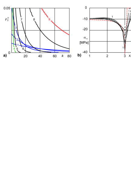
Figure 2: Relative error (a), and normal contact stress (b)

At Fig. 2a the relative error ${\rho}_{2}^{k}$ of displacement $u_{2n}$ on different iterations $k$, obtained for $B=2.5\cdot{10}^{-5}\,\textrm{cm}/(\textrm{MPa})^{a}$, $a=0.5$, is represented for different values of parameter $\gamma$. Curves 1–9 correspond to $\gamma=0.01$, 0.02, 0.05, 0.6, 0.8 (0.3), 0.9, 0.95, 0.98, 0.99. For these values of parameter $\gamma$, DDM (41)–(42) reaches the accuracy $\varepsilon_{u}=10^{-3}$ in 193, 124, 65, 7, 13, 27, 55, 134 iterations respectively.

Thus, we conclude, that the best convergence rate reaches if $\gamma=0.6$. The convergence rate is good if $\gamma\in[\,0.1,\,0.9\,]$. However, it becomes slow when $\gamma$ is close to 0 or to 1. For $\gamma=0.98$ the method is still convergent, but the convergence becomes nonmonotone. For $\gamma\geq 0.99$ the method is not anymore convergent.

At Fig. 2b the normal contact stress ${\sigma}_{1n}={\sigma}_{2n}$, obtained by DDM (41)–(42) for $B=10^{-5}\,\textrm{cm}/(\textrm{MPa})^{a}$ and different values of parameters $a$ is represented. Curves 1–4 correspond to numerical solution for $a=0.3$, 0.6, 0.8, 1. Dashed curve represents the analytical solution, obtained in [13] for contact of two halfspaces without nonlinear layer. Here we conclude, that for small values of $a$ ($a\leq 0.3$) the influence of nonlinear layer on the contact behavior is not so large and the numerical solutions are close to the solution without layer. However, for larger values of $a$ ($a\geq 0.5$) the influence of nonlinear layer becomes more significant and can not be neglected.

The positive feature of proposed domain decomposition methods are the simplicity of their algorithms. These methods have only one iteration loop, which deals with domain decomposition, nonlinearity of Winkler layers and contact conditions.

References

• [1] Bayada, G., Sabil, J., Sassi, T.: A Neumann–Neumann domain decomposition algorithm for the Signorini problem. Applied Mathematics Letters 17(10), 1153–1159 (2004)
• [2] Bresch, D., Koko, J.: An optimization-based domain decomposition method for nonlinear wall laws in coupled systems. Math. Models Methods Appl. Sci. 14(7), 1085–1101 (2004)
• [3] Dostál, Z., Kozubek, T., Vondrák, V., Brzobohatý, T., Markopoulos, A.: Scalable TFETI algorithm for the solution of multibody contact problems of elasticity. Int. J. Numer. Methods Engrg. 41, 675–696 (2010)
• [4] Dyyak, I.I., Prokopyshyn, I.I.: Domain decomposition schemes for frictionless multibody contact problems of elasticity. In: G.K. et al. (ed.) Numerical Mathematics and Advanced Applications 2009, pp. 297–305. Springer (2010)
• [5] Dyyak, I.I., Prokopyshyn, I.I., Prokopyshyn, I.A.: Penalty Robin–Robin domain decomposition methods for unilateral multibody contact problems of elasticity: Convergence results (2012). URL http://arxiv.org/pdf/1208.6478.pdf
• [6] Goryacheva, I.G.: Contact mechanics in tribology. Kluwer (1998)
• [7] Hintermüller, M., Ito, K., Kunisch, K.: The primal-dual active set strategy as semismooth Newton method. SIAM J. OPTIM. 13(3), 865–888 (2003)
• [8] Koko, J.: Convergence analysis of optimization-based domain decomposition methods for a bonded structure. Applied Numerical Mathematics (58), 69–87 (2008)
• [9] Koko, J.: Uzawa block relaxation domain decomposition method for a two-body frictionless contact problem. Applied Mathematics Letters 22, 1534–1538 (2009)
• [10] Prokopyshyn, I.I.: Parallel domain decomposition schemes for frictionless contact problems of elasticity. Visnyk Lviv Univ. Ser. Appl. Math. Comp. Sci. 14, 123–133 (2008). [In Ukrainian]
• [11] Prokopyshyn, I.I., Dyyak, I.I., Martynyak, R.M., Prokopyshyn, I.A.: Penalty Robin–Robin domain decomposition schemes for contact problems of nonlinear elastic bodies (2012). URL http://arxiv.org/pdf/1209.1129.pdf. [Accepted to DD20 Proceedings]
• [12] Sassi, T., Ipopa, M., Roux, F.X.: Generalization of Lion’s nonoverlapping domain decomposition method for contact problems. Lect. Notes Comput. Sci. Eng. 60, 623–630 (2008)
• [13] Shvets, R.M., Martynyak, R.M., Kryshtafovych, A.A.: Discontinuous contact of an anisotropic half-plane and a rigid base with disturbed surface. Int. J. Engng. Sci. 34(2), 183–200 (1996)
• [14] Suquet, P.M.: Discontinuities and plasticity. In: CISM Courses Lect., 302, pp. 279–340 (1988)
• [15] Vorovich, I.I., Alexandrov, V.M. (eds.): Contact Mechanics. Fizmatlit, Moscow (2001)
• [16] Wohlmuth, B.: Variationally consistent discretization schemes and numerical algorithms for contact problems. Acta Numerica 20, 569–734 (2011)