Black Hole spin dependence of general relativistic multi-transonic accretion close to the horizon

Abstract

We introduce a novel formalism to investigate the role of the spin angular momentum of astrophysical black holes in influencing the behaviour of low angular momentum general relativistic accretion. We propose a metric independent analysis of axisymmetric general relativistic flow, and consequently formulate the space and time dependent equations describing the general relativistic hydrodynamic accretion flow in the Kerr metric. The associated stationary critical solutions for such flow equations are provided and the stability of the stationary transonic configuration is examined using an elegant linear perturbation technique. We examine the properties of infalling material for both prograde and retrograde accretion as a function of the Kerr parameter at extremely close proximity to the event horizon. Our formalism can be used to identify a new spectral signature of black hole spin, and has the potential of performing the black hole shadow imaging corresponding to the low angular momentum accretion flow.

,

1 Introduction

Astrophysical black holes are the terminal states of the gravitational collapse of massive celestial objects. They can be conceived as singularities in space time censored by a mathematically defined ‘one way barrier’ – the event horizon, and are not amenable to any direct physical observation. As a result, their presence can only be realized through the gravitational influence they exert on the matter falling onto those objects. The infalling matter inevitably plunges through the event horizon on a relativistic scale of velocity. Given a set of physically realizable outer boundary conditions, such accretion eventually manifests transonic properties in order to obey the inner boundary conditions [1]. Subsonic at a large distance, accretion thus reaches the event horizon supersonically.

The hypothesis that most (if not all) of the supermassive black holes and the stellar mass black holes powering the active galactic nuclei and the galactic microquasars, respectively, possess non-zero values of the spin angular momentum has gained widespread acceptance in recent times [2, 3, 4, 5, 6, 7, 8, 9, 10, 11, 12, 13, 14, 15, 16, 17, 18, 19, 20, 21]. The black hole spin plays a deterministic role in influencing various characteristic features of the dynamical and the spectral features of accretion and related phenomena in the characteristic metric – the energy extraction from a spinning black hole through the Blandford-Znajek Mechanism [22, 23, 13, 24], the spin dependence of the black hole shadow imaging [25, 26, 27, 28, 29, 30, 31], various evolutionary properties of the normal and the active galaxies [32, 33, 34], QPO associated with the Galactic and the extra-galactic sources [35, 36, 37, 38, 39, 40, 41], and the Quasar X-ray micro-lensing [42], to mention a few.

Our investigation of how the black hole spin angular momentum influences the dynamical and the radiative behaviour of the general relativistic transonic accretion at the close vicinity of the event horizon of a rotating black hole has been motivated by the set of works referred in the previous paragraphs. The prime objective of this paper is to investigate what properties of the low angular momentum shocked accretion flow are the principal attributes of the black hole spin in extremely close proximity to the event horizon of a Kerr [43] black hole.

To accomplish our task, we conduct a detailed and multi-step investigation of the transonic properties of general relativistic axisymmetric hydrodynamic inviscid accretion of low angular momentum as realized on the equatorial plane of the Kerr metric using the Boyer Lindquist [44] coordinates. We begin with a general prescription where we consider a four dimensional stationary axisymmetric manifold with two commuting Killing vector fields and subsequently construct the general relativistic Euler and the continuity equations from the appropriate energy momentum tensor. Quite interestingly, we have been able to demonstrate, using certain symmetry arguments, that for the three dimensional submanifold the fluid equations are separable using analytical scheme and the corresponding flow velocity components can be completely determined once the equation of state is specified. We thus formulate a general framework for studying the equations for fluid flow in a rotating black hole spacetime.

The transonic flow properties in the phase portrait, however, can not be determined analytically because of certain issues which will be elaborated in the subsequent sections. The emergence of the multi-transonic behaviour manifests through the critical point analysis. Such multi-transonic accretion solution, as we will see in the subsequent sections, may contain a stationary shock, properties of which are obtained by the explicit solution of the general relativistic Rankine-Hugoniot conditions. The properties of the post shock flow are then studied as a function of the black hole spin – the Kerr parameter, $a$. The post shock flow solutions are then followed up to a sufficiently close proximity of the event horizon to demonstrate how the terminal values of the shocked accretion variables are influenced by the black hole spin angular momentum, and the consequences of such dependence are discussed in detail.

The entire formalism developed to study the spin dependence of the behaviour of accreting matter close to the event horizon as described above is based on the stationary integral solutions of the differential equations describing the accretion phenomena. Along with the understanding of the transonic behaviour of the stationary flow solutions, it is rather necessary to ensure the stability of such stationary configurations. This stability study can be accomplished by studying the time evolution of a linear acoustic like perturbation in the full time dependent flow equations. The existence of the stable stationary transonic solution is associated with the non-divergent amplitude of the linear perturbation of such category. In this work, we develop a novel perturbation scheme applicable to the axisymmetric potential flow as realized on the equatorial plane of the Kerr metric. We perturb the velocity potential corresponding to the advective velocity of the low angular momentum accretion considered in our work and demonstrate that such perturbations do not diverge for astrophysically relevant time scales. We thus formally establish the consistency of the formalism, which, for the first time in the literature, has been introduced in the present work to study the black hole spin dependence of the terminal behaviour of shocked accreting material very close to the event horizon of a Kerr black hole.

2 Multi-transonicity in black hole accretion: retrospective and contemporary aspects

For accretion onto astrophysical black holes, the transonicity is characterized by a transition from the subsonic state ($M<1$, where $M$ is the Mach number of the flow) to the supersonic state ($M>1$), or vice versa. For the present work, the Mach number $M$ is considered to be the local radial Mach number for stationary transonic accretion solutions and is defined to be the ratio of the local advective velocity $u$ (defined in subsequent sections) and the local speed of the propagation of the acoustic perturbation (local barotropic sound speed) $c_{s}$ as defined in subsequent sections. Such a transition may be a regular one through the sonic point and is associated with the transition of $M<1\longrightarrow M>1$ type or may be a discontinuous one through a stationary shock and is associated with the $M>1\longrightarrow M<1$ type transition. The non linear equations describing the steady, inviscid stationary axisymmetric flow can be tailored to form a first order autonomous dynamical system [45, 46, 47, 48]. The physical transonic accretion solution for the stationary axisymmetric flow can formally be realized as critical solution on the phase portrait spanned by $M$ and the radial distance $r$ measured along the equatorial plane – see, e.g., [49, 50] and references therein.

For low angular momentum sub-Keplerian accretion, such transonic features may be exhibited more than once on the phase portrait of the stationary solutions. Such multi-transonicity as well as the resulting shock formation phenomena for axisymmetric accretion under the influence of various post Newtonian potentials, mainly, under the influence of the Paczyński–Wiita [51] pseudo-Schwarzschild potential, has been widely studied in the literature, see e.g., [1, 54, 55, 56, 57, 58, 59, 60, 53, 61, 62] and references therein.

A regular stationary accretion solution cannot encounter more than one transonic points. A multi-transonicity implies a particular flow configuration with three critical points where two transonic solutions through two different saddle type critical points are connected by a discontinuous stationary shock transition. The inner boundary condition imposed by the event horizon indicates that such a combined multi-transonic shocked solution originates from a large distance as a subsonic flow and encounters the outermost saddle type sonic point to become supersonic for the fist time. Subjected to the appropriate initial boundary conditions, such supersonic flow makes a $M>1\longrightarrow M<1$ type discontinuous transition through a stationary shock and the shock induced subsonic flow becomes supersonic again at the innermost saddle type sonic point.

One expects that a shock formation in black-hole accretion discs might be a general phenomenon because shock waves in rotating astrophysical flows potentially provide an important and efficient mechanism for conversion of a significant amount of the gravitational energy into radiation by randomizing the directed infall motion of the accreting fluid. Hence, the shocks play an important role in governing the overall dynamical and radiative processes taking place in astrophysical fluids accreting onto black holes. The hot and dense post shock flow is considered to be a powerful diagnostic tool in understanding various astrophysical phenomena [63, 64, 65, 66, 67, 35, 37, and references therein].

The idea of shock formation in black hole accretion flow has been, however, contested by some authors (see, e.g., [68] and references therein for a review). Nevertheless, the issue of not finding shocks in such works perhaps lies in the fact that only one sonic point close to the black hole may usually be explored using the framework of the shock free advection dominated accretion flow solutions. Also to be emphasized is that the concept of low angular momentum flow (capable of providing the favourable configuration of the formation of standing shock) is not a theoretical abstraction and sub-Keplerian flows are observed in nature as reality. Such flow configurations may be observed for detached binary systems fed by accretion from OB stellar winds [69, 70], semi-detached low-mass non-magnetic binaries [71], and super-massive black holes fed by accretion from slowly rotating central stellar clusters [72, 73, and references therein]. Even for a standard Keplerian accretion disc, turbulence may produce such low angular momentum flow [see, e.g. 74, and references therein].

Multi-transonicity in black hole accretion has been addressed using the general relativistic framework as well. The legacy of the pioneering contributions by [75] and [76] to study the general relativistic axisymmetric black hole accretion in the Kerr metric followed two different avenues, quite often in a non overlapping fashion. One school of thought essentially studied the transonic accretion without paying much attention to the appearance of the multi-transonicity and the formation of shock, but rather putting emphasis on other crucial behaviours of the flow, see, e.g., [77, 78, 79, 80, 81, 82, 83, 84, 85], and references therein.

The appearance of the multiple critical points in general relativistic flow onto a spinning black hole was observed and consequently the formation of the standing shock has been conjectured in the alternative set of (sometime contesting the aforementioned category of work dealing with accretion flow without the appearance of shock transition) literature, with the main motivation to explain the spectral state by incorporating the physics of the post shock accretion flow, as already mentioned. The profound work by [86] is credited to be the first ever comprehensive work in the literature which provides the complete formalism for the shock formation in a general relativistic multi-critical accretion flow, although it is worth mentioning that even before [86], multiplicity in the critical points for the general relativistic axisymmetric flow was addressed [87, 88] without mentioning the issue of the shock formation. By revisiting the concept of the Keplerian circular motion for rotating fluids in general relativity. [89] intuitively explained certain issues related to the shock formation for multi-transonic accretion onto a Kerr black hole.

The full general relativistic formalism introduced by [87, 88] and [86] was followed by [90, 91] where a non relativistic calculation for the shock formation for accretion and other related issues were erroneously incorporated within the relativistic framework and some of the results valid for the isothermal flow had directly been applied to study the polytropic flow without appropriate justification. [92, 93, 94, 95] used the general relativistic shock condition to study the multi-transonic flow for the conical model. [81] studied the general relativistic accretion for multi-transonic flow but the shock formation mechanism was not studied in sufficient detail. While all the above works concentrated on polytropic accretion, shock transitions in general relativistic isothermal flows were discussed in [96, 97, 98]. Shocked accretion for MHD flows in Kerr geometry has also been studied [99, 100, 101].

Meanwhile, it was realized that it is instructive to incorporate an expression for the flow thickness for flow in hydrostatic equilibrium in the vertical direction such that the corresponding flow equation will remain non singular on the horizon. Both the thin accretion disc as well as the quasi-spherical flow structure can be accommodated using such a disc height. [102] provided such an expression for the general flow structure. The disc height introduced by [102] had further been modified to study the multi-transonic flow structure around Kerr black holes in [103, 50, 104].

Owing to the strong curvature of space time close to the black hole, accreting fluid is expected to manifest extreme behaviour just before plunging into the event horizon. The spectral signature of this tremendously hot ultra fast matter with its characteristic density and pressure profile is expected to provide the key features of the strong gravity space time to the close proximity of the event horizon. A detailed study of the role of the black hole spin angular momentum in influencing the dynamical features of the transonic matter close to the event horizon is thus very important to perform to understand the salient features of the general relativistic black hole space time, and, in turn, to understand the physical properties of the Kerr metric itself. [82] and [83] were the first to make attempt to understand the flow properties close to the black hole by studying the general relativistic optically thin advection dominated accretion flow (ADAF) in the Kerr metric. Later on, [105] applied the method of post Newtonian asymptotic analysis to investigate the properties of the inner region of ADAF to obtain their results that has been argued to be in agreement with the relativistic flow description. Subsequently, [103] studied the influence of black hole spin in determining the properties of the accretion variables sufficiently close to the event horizon for multi-transonic flow, although the shock conditions were not taken into account in their work. It has recently been demonstrated that the multi-transonicity can only be realized through the presence of a standing shock since a smooth flow can never make more than one regular sonic transition [104].

We would like to study the behaviour of the low angular momentum multi-transonic shocked accretion extremely close to the black hole event horizon. The present work differs from all previous works on general relativistic accretion, including [82, 83] and [103]. Not only a multi-transonic shocked flow has been studied at the close vicinity of the event horizon to understand the role of the black hole spin angular momentum on determining the salient features of such flow, a complete description of the linear perturbation analysis has also been provided in our present paper which ensures the stability of such accretion solutions. In addition, a formal analytical description for the general fluid flow in axisymmetric black hole space time has also been provided.

We introduce the stationary integral flow solutions with standing shocks by solving the relativistic Rankine-Hugoniot conditions, and study the behaviour of the post shock flow upto the very close proximity of the horizon. We then compare such results with the hypothetical flow solutions for which the flow would not pass through a shock (and hence would behave like a mono-transonic flow passing through the saddle type outermost sonic point formed at a large distance from the black hole event horizon) for the same set of initial boundary conditions describing the flow. This allows us to understand whether the shock formation phenomena can alter the dynamical and thermodynamic state of matter extremely close to the event horizon and whether such change may show up through the spectral properties of the black hole candidates.

From recent theoretical and observational findings, the relevance of the counter-rotating accretion in black hole astrophysics is being increasingly evident [11, 12, 13, 106]. It is thus instructive to study whether the characteristic features of the terminal values of the accretion variables for the prograde flow differ considerably from those of the retrograde flow. To the best of our knowledge, our work presents the first detailed spin dependence of the terminal behaviour of infalling matter for retrograde accretion onto a Kerr black hole using the complete general relativistic framework, as well as study the comparison between the prograde and the retrograde flow in this context.

We, however, do not explicitly consider the viscous transport of the angular momentum and the specific angular momentum of the accretion flow has been taken to be invariant. Reasonably large radial advective velocity for the slowly rotating sub-Keplerian flow implies that the infall time scale is considerably shorter than the viscous time scale for the flow profile considered in this work. Large radial velocities even at larger distances are due to the fact that the angular momentum content of the accreting fluid is relatively low [107, 108, 109]. The assumption of inviscid flow for the accretion profile under consideration may thus be justified from an astrophysical point of view. Such inviscid configuration has also been addressed by other authors using detailed numerical simulation works [109, 110, 67].

3 Metric independent formulation of velocity profile for most general axisymmetric spacetime

We consider a generic (3+1) stationary axisymmetric space-time endowed with two commuting Killing vector fields, within which the three dimensional general relativistic fluid (without the back reaction) field will be examined. In such a space-time, the combined Euler and the continuity equation take the form

$$v^{\mu}\nabla_{\mu}v^{\nu}+\frac{c_{s}^{2}}{\rho}\nabla_{\mu}\rho\left(g^{\mu\nu}+v^{\mu}v^{\nu}\right)=0,$$ (1)

where $v^{\mu}$ is the time like fibre bundle (a tangent vector field in the present context) defined on the manifold constructed by the family of streamlines. The normalisation condition corresponding to the velocity vector field $v^{\mu}$ is taken to be $v^{\mu}v_{\mu}=-1$. $c_{s}$ is the speed of propagation of the acoustic perturbation embedded in the accreting fluid and $\rho$ is the local rest mass energy density of the fluid. For a single temperature fluid $\rho$ can be replaced by the particle number density.

For a stationary axisymmetric manifold of dimension four endowed with two Killing vector fields $\xi^{\mu}$ and $\phi^{\mu}$ one has

$$\nabla_{(_{\mu}\xi_{\nu})}=0=\nabla_{(_{\mu}\phi_{\nu})}$$ (2)

The locally timelike Killing vector field $\xi^{\mu}$ (of norm $\varsigma$) is the generator of stationarity whereas the locally spacelike Killing field $\phi^{\mu}$ (of norm $\varphi$) with closed spacelike integral curves generates the axisymmetry. It is usually not possible to obtain any orthogonal basis for the space-time of our consideration since $\xi_{\mu}\phi^{\mu}\neq 0$ for stationary axisymmetric space-time. We would intend to specify an orthogonal basis using which the space time metric can directly be expressed. To accomplish such task we first define

$$\Upsilon_{\mu}:=\xi_{\mu}-\frac{(\xi.\phi)}{(\phi.\phi)}\phi_{\mu}\equiv\xi_{\mu}-\iota\phi_{\mu},$$ (3)

and it is generically observed that $\Upsilon_{\mu}\phi^{\mu}=0$. Norm of $\Upsilon^{\mu}$ can thus be expressed as,

$$\Upsilon_{\mu}\Upsilon^{\mu}=-(-\varsigma^{2}+\iota^{2}\varphi^{2})=-\varpi^{2},$$ (4)

where $\Upsilon_{\mu}$ is timelike and $\varpi^{2}$ is positive. The metric element can now be expressed in the orthogonal bases as follows

$$g_{\mu\nu}=-\varpi^{-2}\Upsilon_{\mu}\Upsilon_{\nu}+\varphi^{-2}\phi_{\mu}\phi_{\nu}+R^{-2}R_{\mu}R_{\nu}+\vartheta^{-2}\Theta_{\mu}\Theta_{\nu},$$ (5)

$\left\{R^{\mu},\Theta^{\mu}\right\}$ being the spacelike basis vectors orthogonal to $\left\{\Upsilon^{\mu},\phi^{\mu}\right\}$. For a stationary axisymmetric space-time the hypersurface $\varsigma^{2}=0$ defines an ergosphere rather than the horizon. $\varsigma^{2}$ is negative inside the ergosphere since $\xi^{\mu}$ is spacelike in that region. On the other hand, a compact $\varpi^{2}=0$ hypersurface defines a Killing horizon which is a black hole event horizon for our consideration. This can be demonstrated by constructing the null geodesic congruence on such a surface.

The formalism developed in the previous paragraphs is valid for a very general kind of stationary axisymmetric space-time, which includes, but certainly not limited to, the space-time defined by the Kerr family of solutions. With reference to eq. (5), the normalisation condition for velocity vector field may be expressed as

$$v^{\mu}v^{\nu}g_{\mu\nu}=-\varsigma^{-2}v_{0}^{2}+\varphi^{-2}v_{1}^{2}+R^{-2}v_{2}^{2}+\vartheta^{-2}v_{3}^{2}=-1,$$ (6)

where $v_{0}=v_{\mu}\Upsilon^{\mu}$ etc. are scalars. Contracting the equation (1) with $\xi^{\mu}$ we obtain

$$v^{\mu}\nabla_{\mu}(v^{\nu}\xi_{\nu})+\frac{c_{s}^{2}}{\rho}\left[\xi^{\mu}\nabla_{\mu}\rho+(\xi_{\mu}v^{\mu})v^{\nu}\nabla_{\nu}\rho\right]=0,$$ (7)

where $v^{\mu}v^{\nu}\nabla_{\mu}\xi_{\nu}=\frac{1}{2}v^{\mu}v^{\nu}\nabla_{(_{\mu}\xi_{\nu})}=0$ is ensured by virtue of the killing equation, i.e. eq. (2). Through similar procedure we also obtain

$$v^{\mu}\nabla_{\mu}v_{1}+\frac{c_{s}^{2}}{\rho}\left[\phi^{\mu}\nabla_{\mu}\rho+v_{1}v^{\nu}\nabla_{\nu}\rho\right]=0.$$ (8)

Note that all the differential terms appearing in Eqs. (7-8) involve partial derivatives only, since $v_{\mu}\xi^{\mu}$ and $v_{1}$ are scalars.

Since we consider the stationary, axisymmetric flow in three dimensions, all the directional partial derivatives with respect to $\xi^{\mu}$ and $\phi^{\mu}$ vanishes to yield,

$$\frac{\mathrm{d}v_{1}}{\mathrm{d}R}+\frac{c_{s}^{2}}{\rho}v_{1}\frac{\mathrm{d}\rho}{\mathrm{d}R}=0,$$ (9)

from eq. (8), $R$ being a parameter along $R^{\mu}$. Integration of eq. (9) provides

$$v_{1}=\mathcal{A}\exp{\left(-\int\frac{c_{s}^{2}}{\rho}\mathrm{d}R\right)},$$ (10)

$\mathcal{A}$ being a constant to be evaluated using the initial boundary conditions.

In a similar fashion, eq. (7) provides the expression for $v_{\mu}\xi^{\mu}$, which will formally be same as $v_{1}$ upto an integration constant, since $\xi^{\mu}$ is a Killing vector field. One thus finds,

$$v_{0}=v_{\mu}\xi^{\mu}-\iota v_{\mu}\phi^{\mu}.$$ (11)

Substitution of $v_{0}$ from eq. (11) and $v_{1}$ from eq. (10) into eq. (6) provides the expression of $v_{2}$.

In this section we thus provide a general formalism for evaluating all relevant bulk velocity components of a rotating accretion flow in a most general axisymmetric space-time. $\left\{v_{0},v_{1},v_{2}\right\}$ are, however, the general solutions and exact estimation of their specific numerical values for a particular flow configuration in a predetermined black hole metric is a rather involved procedure since the integration constant appearing in the expressions of $\left\{v_{0},v_{1},v_{2}\right\}$ can be evaluated if and only if the appropriate set of the initial boundary conditions are provided. More importantly, the sound speed as well as the rest mass energy density is to be known a priori to find the specific values of $\left\{v_{i}\right\}$. For our specific purpose, however, the axisymmetric space-time metric is of Kerr type, and $\left\{v_{i}\right\}\equiv\left\{v_{t},v_{r},v_{\theta},v_{\phi}\right\}$, for which, the initial boundary conditions cannot be evaluated analytically for barotropic equation of state and for a certain geometric configuration of the accreting fluid. $c_{s}$ and $\rho$ are not specified a priori.

Procedure described in this section so far for finding the general solution of $\left\{v_{i}\right\}$ is thus useful for the flow configuration with known value of $\left\{c_{s},\rho\right\}$ and initial boundary conditions. Axisymmetric low angular momentum accretion onto an astrophysical black hole however constitutes a complex gravitational system for which such predetermined set of information is not readily available in general. In subsequent sections, we thus plan to develop a metric specific formalism to understand the spatial velocity profile of the stationary axisymmetric flow.

4 Space-time metric and the conservation equations

Hereafter, radial distances will be scaled in units of $GM_{BH}/c^{2}$ and associated will be scaled by $c$, where $G$, $M_{BH}$ and $c$ are universal gravitational constant, mass of the black hole and speed of light in vacuum, respectively. $G=c={\mathbf{M}_{BH}}=1$ is adopted. The allowed domain of $a$, the Kerr parameter is taken as $-1<a<1$ as usual.

Using Boyer-Lindquist [44] co-ordinates, the corresponding metric element for the Kerr family of solutions in the spherical polar co-ordinate can be expressed as

$$\mathrm{d}s^{2}=-\left(1-\frac{2}{\mu r}\right)\mathrm{d}t^{2}+\frac{\mu r}{\Delta}\mathrm{d}r^{2}+ \mu r^{2}\mathrm{d}\theta^{2}-\frac{4a\sin^{2}\theta}{\mu r}\mathrm{d}t\mathrm{d}\phi$$

$$+r^{2}\sin^{2}\theta\left(1+\frac{a^{2}}{r^{2}}+\frac{2a^{2}\sin^{2}\theta}{\mu r^{3}}\right)\mathrm{d}\phi^{2},$$ (12)

where $\theta$ is the polar angle, $\mu=1+\frac{a^{2}}{r^{2}}\cos^{2}\theta$ and $\Delta=r^{2}-2r+a^{2}$.

The corresponding covariant metric components are obtained as

$$g_{tt} =-\left(1-\frac{2}{\mu r}\right).\;\;\;g_{rr}=\frac{\mu r^{2}}{\Delta}.\;\;\;g_{\theta\theta}=\mu r^{2},$$

$$g_{t\phi} =g_{\phi t}=-\frac{2a\sin^{2}\theta}{\mu r}.$$

$$g_{\phi\phi} =r^{2}\sin^{2}\theta\left(1+\frac{a^{2}}{r^{2}}+\frac{2a^{2}\sin^{2}\theta}{\mu r^{3}}\right).$$

Associated contravariant elements can thus be written as

$$g^{tt} =-\frac{g_{\phi\phi}}{g_{t\phi}^{2}-g_{tt}g_{\phi\phi}}=-\left[1+\frac{2r}{\mu\Delta}\left(1+\frac{a^{2}}{r^{2}}\right)\right],$$

$$g^{rr} =\frac{1}{g_{rr}}=\frac{\Delta}{\mu r^{2}},$$

$$g_{\theta\theta} =\frac{1}{g_{\theta\theta}}=\frac{1}{\mu r^{2}},$$

$$g^{t\phi} =g^{\phi t}=\frac{g_{t\phi}}{g_{t\phi}^{2}-g_{tt}g_{\phi\phi}}=-\frac{2a}{\mu\Delta r},$$

$$g^{\phi\phi} =-\frac{g_{\phi\phi}}{g_{t\phi}^{2}-g_{tt}g_{\phi\phi}}=-\frac{\left(1-\frac{2}{\mu r}\right)}{\Delta\sin^{2}\theta}.$$

We, however, will be working on the stationary flow configuration on the equatorial plane (as defined by $|\theta-\pi/2|\ll 1$ in [76]. The line element on the equatorial slice is expressed as

$$\mathrm{d}s_{eq}^{2}=(g_{tt})_{eq}\mathrm{d}t^{2}+(g_{rr})_{eq}\mathrm{d}r^{2}+(g_{\theta\theta})_{eq}\mathrm{d}\theta^{2}+2(g_{t\phi})_{eq}\mathrm{d}t\mathrm{d}\phi+(g_{\phi\phi})_{eq}\mathrm{d}\phi^{2};$$ (13)

where the subscript ‘$eq$’ implies that the corresponding values are evaluated at the equatorial plane.

Hence,

$$(g_{tt})_{eq} =-\left(1-\frac{2}{r}\right),$$ (14a)

$$(g_{rr})_{eq} =\frac{r^{2}}{\Delta},$$ (14b)

$$(g_{\theta\theta})_{eq} =r^{2},$$ (14c)

$$(g_{t\phi})_{eq} =(g_{\phi t})_{eq}=-\frac{2a}{r},$$ (14d)

$$(g_{\phi\phi})_{eq} =\frac{A}{r^{2}};$$ (14e)

where $A=r^{4}+r^{2}a^{2}+2ra^{2}$. The corresponding contravariant metric elements can thus be evaluated as,

$$(g^{tt})_{eq} =-\frac{(g_{\phi\phi})_{eq}}{(g_{t\phi})_{eq}^{2}-(g_{tt})_{eq}(g_{\phi\phi})_{eq}}=-\frac{A}{\Delta r^{2}},$$ (15a)

$$(g^{rr})_{eq} =\frac{1}{(g_{rr})_{eq}}=\frac{\Delta}{r^{2}},$$ (15b)

$$(g_{\theta\theta})_{eq} =\frac{1}{(g_{\theta\theta})_{eq}}=\frac{1}{r^{2}},$$ (15c)

$$(g^{t\phi})_{eq} =\frac{(g_{t\phi})_{eq}}{(g_{t\phi})_{eq}^{2}-(g_{tt})_{eq}(g_{\phi\phi})_{eq}}=-\frac{2a}{\Delta r},$$ (15d)

$$(g^{\phi\phi})_{eq} =-\frac{(g_{\phi\phi})_{eq}}{(g_{t\phi})_{eq}^{2}-(g_{tt})_{eq}(g_{\phi\phi})_{eq}}=-\frac{\left(1-\frac{2}{r}\right)}{\Delta}.$$ (15e)

Hereafter we drop all the ‘$eq$’ subscripts for the sake of brevity. Any $g_{\mu\nu}$ or $g^{\mu\nu}$ will thus explicitly imply that the corresponding metric element has been evaluated on the equatorial plane. Using the cylindrical polar co-ordinate the corresponding metric on the equatorial plane can be expressed as,

$$\mathrm{d}s^{2} =g_{\mu\nu}\mathrm{d}x^{\mu}\mathrm{d}x^{\nu}$$

$$=-\frac{r^{2}\Delta}{A}\mathrm{d}t^{2}+\frac{r^{2}}{\Delta}\mathrm{d}r^{2}+\frac{A}{r^{2}}\left(\mathrm{d}\phi-\omega\mathrm{d}t\right)+\mathrm{d}z^{2},$$ (16)

where $z=r\cos\theta$, $\omega=2ar/A$ and $g_{zz}=1$.

For the metric element expressed using $(r,\theta,\phi)$, $g_{(r,\theta,\phi)}\equiv\det(g_{\mu\nu})=-r^{4}$, whereas for $\mathrm{d}s^{2}$ expressed using $(r,\phi,z)$, $g_{(r,\phi,z)}=-r^{2}$. Calculations presented in this work will mainly be based on the line element as expressed in eq. (16).

In this work, the polytropic equation of state of the following form

$$p=K\rho^{\gamma}$$ (17)

is considered to describe the flow, where the polytropic index $\gamma$ (which is equal to the ratio of the specific heat, at constant pressure and volume, $C_{p}$ and $C_{v}$, respectively) of the accreting material is assumed to be constant throughout the fluid. A more realistic flow model would perhaps requires the implementation of a variable polytropic index having a functional dependence on the radial distance of the form $\gamma\equiv\gamma(r)$ [111, 112]. However, we have performed our calculations for a reasonably broad spectrum of $\gamma$ and thus believe that all astrophysically relevant polytropic indices are covered in our analysis.

The proportionality constant $K$ in Eq. (17) is related to the specific entropy of the accreting fluid (provided no additional entropy generation takes place). Subjected to the condition that the Clapeyron equation of the form ($k_{B}$, $\mu$ and $m_{p}\sim m_{H}$ being the locally measured flow temperature, the mean molecular weight, and the mass of the singly ionised hydrogen atom, respectively)

$$p=\frac{k_{B}}{\mu m_{p}}\rho T,$$ (18)

holds in addition to Eq. (17)). The entropy per particle of an ensemble may be expressed as [113]

$$\sigma=\frac{1}{\gamma-1}\log K+\frac{\gamma}{\gamma-1}+{\rm constant};$$

where the constant depends on the chemical composition of the accreting matter. $K$ in eq. (17) can now be interpreted as a measure of the specific entropy of the accreting matter.

The specific enthalpy $h$ is formulated as

$$h=\frac{p+\epsilon}{\rho},$$ (19)

where the energy density $\epsilon$ includes the rest mass density and internal energy, and

$$\epsilon=\rho+\frac{p}{\gamma-1}.$$ (20)

Using expression of $\epsilon$ from Eq. (20) and the expression of $p$ from Eq. (17), the expression for specific enthalpy $h$, as formulated in Eq. (19), turns out to be

$$h=1+\frac{\gamma K\rho^{\gamma-1}}{\gamma-1}$$ (21)

The adiabatic sound speed $c_{s}$ is defined as

$$c_{s}^{2}=\left(\frac{\partial p}{\partial\epsilon}\right)_{\rm h}.$$ (22)

The specific enthalpy may thus be written in terms of $c_{s}^{2}$ as

$$h=\frac{\gamma-1}{\gamma-(1+c_{s}^{2})}.$$ (23)

The energy-momentum tensor of an ideal fluid is introduced as

$$T^{\mu\nu}=(\epsilon+p)v^{\mu}v^{\nu}+pg^{\mu\nu}.$$

Vanishing of the four divergence of the energy momentum tensor provides the general relativistic version of the Euler equation i.e.

$$T^{\mu\nu}_{;\nu}=0.$$ (24)

The continuity equation is obtained from

$$\left(\rho v^{\mu}\right)_{;\mu}=0.$$ (25)

We have defined two Killing vectors $\xi^{\mu}=\delta^{\mu}_{t}$ and $\phi^{\mu}=\delta^{\mu}_{\phi}$ corresponding to stationarity and axisymmetry of the flow, respectively.

We now contract Eq. (24) with $\phi^{\mu}$ to obtain,

$$\phi_{\mu}\left[(\epsilon+p)v^{\mu}v^{\nu}\right]_{;\nu}+\phi_{\mu}p_{,\nu}g^{\mu\nu}=0.$$

But $\phi^{\nu}p_{,\nu}=0$ due to axisymmetry, hence

$$\phi_{\mu}\left[(\epsilon+p)v^{\mu}v^{\nu}\right]_{;\nu}=0,$$

which further provides,

$$g_{\mu\phi}\left[(\epsilon+p)v^{\mu}v^{\nu}\right]_{;\nu}=0,$$ (26)

since $\phi^{\mu}=\delta^{\mu}_{\phi}$. Since $g_{\mu\lambda;\nu}=0,$ Eq. (26) can be written as

$$\left[g_{\mu\phi}(\epsilon+p)v^{\mu}v^{\nu}\right]_{;\nu}=0;$$

from where we obtain

$$\left[\phi_{\mu}hv^{\nu}\right]_{;\nu}=0.$$ (27)

From Eq. (27) one thus infers $\phi_{\mu}hv^{\mu}=hv_{\phi}$. Hence $hv_{\phi}$, the angular momentum per baryon for the axisymmetric flow, is conserved.

It can also be shown (see, e.g., [114] and references therein) that the quantity $v_{\phi}v^{t}$, which is the angular momentum per unit inertial mass, is conserved for an iso-entropic flow. The world lines along which $v_{\phi}v^{t}$ remains constant is a solution of the general relativistic Euler equation.

In a similar way, we contract Eq.(24) with $\xi^{\mu}$

$$\xi_{\mu}T^{\mu\nu}_{;\nu}=0,$$

to demonstrate that $hv_{t}$ to be another conserved quantity. Hereafter, $hv_{t}$ will be interpreted as the specific energy of the flow and will be denoted be $\mathcal{E}$ (scaled in units of $m_{0}c^{2}$ using the system of units adopted in this work). For polytropic adiabatic accretion, $\mathcal{E}$ is a first integral of motion along a streamline, and can be identified with the relativistic Bernoulli’s constant [115].

The angular velocity of the flow $\Omega$ can be defined in terms of the specific angular momentum $\lambda$, where

$$\lambda=-\frac{v_{\phi}}{v_{t}},$$

as

$$\Omega=\frac{v^{\phi}}{v^{t}}=-\frac{g_{t\phi}+g_{tt}\lambda}{g_{\phi\phi}+g_{t\phi}\lambda}=\frac{r\left[2a+\lambda(r-2)\right]}{A-2a\lambda r}.$$

The normalisation condition $v^{\mu}v_{\mu}=-1$ provides

$$v^{t}v_{t}+v^{r}v_{r}+v^{\phi}v_{\phi}=-1.$$

In terms of the angular velocity $\Omega$ and the specific angular momentum $\lambda$, one writes

$$v^{t}v_{t}+v^{r}v_{r}+\Omega v^{t}(-\lambda v_{t})=-1$$ (28)

Since $v^{2}\equiv-\frac{v^{r}v_{r}}{v^{t}v_{t}}$, one re writes eq. (28) as

$$v^{t}v_{t}(1-\lambda\Omega-v^{2})=-1.$$

By converting $v^{t}\rightarrow v_{t}$) one obtains

$$(g^{tt}-\lambda g^{t\phi})(1-\lambda\Omega-v^{2})v_{t}^{2}=-1$$

. Using the definition of $\Omega$, we show

$$\left(\frac{g_{\phi\phi}+\lambda g_{t\phi}}{g_{t\phi}^{2}-g_{tt}g_{\phi\phi}}\right)(1-\lambda\Omega-v^{2})v_{t}^{2}=1,$$

hence the advective velocity $u$ is related to the three velocity $v$ through $u=v/\sqrt{1-\lambda\Omega}$ (The advective velocity, i.e. the radial velocity of the fluid is measured in a frame which co-rotates with the fluid such that $v^{r}=u/\sqrt{g_{rr}(1-u^{2})}$, see [82]). We find

$$v_{t}=\sqrt{\frac{g_{t\phi}^{2}-g_{tt}g_{\phi\phi}}{(1-\lambda\Omega)(1-u^{2})(g_{\phi\phi}+\lambda g_{t\phi})}}.$$ (29)

The mass conservation equation (the continuity equation as defined by eq. (25)) provides

$$\frac{1}{\sqrt{-g}}(\sqrt{-g}\rho v^{\mu})_{,\mu}=0,$$ (30)

where $g\equiv\det(g_{\mu\nu})$. We multiply equation (30) with the co-variant volume element $\sqrt{-g}\mathrm{d}^{4}x$ to obtain

$$(\sqrt{-g}\rho v^{\mu})_{,\mu}\mathrm{d}^{4}x=0.$$

Note that $\partial_{t}$ and $\partial_{\phi}$ are not relevant due to the stationarity and axisymmetry. following the assumption of non-existence of a convection current along any non-equatorial direction, no non-zero terms involving $v^{\theta}$ (for spherical polar co-ordinates) or $v^{z}$ (for flow studied within the framework of cylindrical co-ordinates) may be considered. We have

$$\partial_{r}(\sqrt{-g}\rho v^{r})\mathrm{d}r\mathrm{d}\theta\mathrm{d}\phi=0,$$ (31)

for accretion studied using the spherical polar co-ordinate and

$$\partial_{r}(\sqrt{-g}\rho v^{r})\mathrm{d}r\mathrm{d}z\mathrm{d}\phi=0,$$ (32)

for accretion studied using the cylindrical co-ordinate.

One can integrate eq. (31) for $\phi=0\rightarrow 2\pi$ and $\theta=[(\pi/2)-H_{\theta}]\rightarrow[(\pi/2)+H_{\theta}]$; $\pm H_{\theta}$ being the range of variation of the polar co-ordinate below and above the equatorial plane, respectively, for a (local) flow half thickness $H$. The ratio $2H/r$ is constant for flow thickness in spherical polar co-ordinate for conical wedge shaped flows, [see e.g. 54, 82, 89, 92, 93, 94, 116, and references within]. Eq. (32) can be integrated for $z=-H_{z}\rightarrow H_{z}$ (where $\pm H_{z}$ is the local half thickness of the flow) symmetrically over and below the equatorial plane for axisymmetric accretion studied using the cylindrical polar co-ordinate to obtain the conserved mass accretion rate $\dot{M}$ in the equatorial plane as

$$\rho v^{r}\mathcal{A}(r)=\dot{M};$$ (33)

$\mathcal{A}(r)$ is the surface area through which the inward mass flux is estimated. For spherical symmetry, $\mathcal{A}(r)=4\pi H_{\theta}r^{2}$ (for not very large values of $\theta$) and for cylindrical symmetry, $\mathcal{A}(r)=4\pi H_{z}r$.

In standard literature of accretion astrophysics, the local flow thickness for an inviscid axisymmetric flow can vary in three different ways, with different degrees of complexity, (see, e.g. [116], and references therein). A constant flow thickness is considered for simplest possible flow configuration where the disc height $H$ is not a function of the radial distance [117]. In its next variant, the axisymmetric accretion can have a conical wedge shaped structure ([54], [87, 88, 89, 92, 93, 94, 95]) where $H$ is directly proportional to the radial distance as $H=A_{h}r$. The geometric constant $A_{h}$ is determined from the measure of the solid angle subtended by the flow. For the hydrostatic equilibrium in the vertical direction, [118, 119, 37, and references therein] the expression for the local flow thickness can have a rather complex dependence on the radial distance and on the local speed of propagation of the acoustic perturbation embedded inside the accretion flow. In the present work, we consider the accretion flow to be in vertical equilibrium, and assume that the flow has a radius-dependent local thickness with its central plane coinciding with the equatorial plane of the black hole. The equations [103] of motion apply to the equatorial plane of the black hole, whereas the hydrodynamic flow variables are averaged over the half thickness of the disc $H$. We follow [102] to derive the disc height for our flow configuration, and obtain the expression for the local flow thickness to be

$$H(r)=\sqrt{\frac{2}{\gamma+1}}r^{2}\left[\frac{(\gamma-1)c_{s}^{2}}{\left\{\gamma-(1+c_{s}^{2})\right\}\left\{\lambda^{2}v_{t}^{2}-a^{2}(v_{t}-1)\right\}}\right]$$

. Using the expression for $v_{t}$ as obtained from its expression in eq. (29) (using the expressions for $g_{\mu\nu}$’s at equatorial plane as mentioned on Eqs. (14)), i.e., by writing $v_{t}$ as

$$v_{t}=\left[\frac{Ar^{2}\Delta}{(1-u^{2})(A^{2}-4a\lambda rA+\lambda^{2}r^{2}(4a^{2}-r^{2}\Delta))}\right]^{\frac{1}{2}},$$

$H(r)$ can be obtained in terms of the advective velocity $u$.

5 Critical point conditions

We derive the two first integrals of motion, the conserved specific energy ${\cal E}$ of the flow and the mass accretion rate ${\dot{M}}$, respectively (using the expressions of $h$, $v_{t}$ and $v^{r}$ as obtained from the preceding section) as

$${\cal E}=\left[\frac{(\gamma-1)}{\gamma-(1+c^{2}_{s})}\right]\sqrt{\left(\frac{1}{1-u^{2}}\right)\left[\frac{Ar^{2}\Delta}{A^{2}-4\lambda arA+\lambda^{2}r^{2}(4a^{2}-r^{2}\Delta)}\right]}\,,$$ (34)

$${\dot{M}}=4{\pi}{\Delta}^{\frac{1}{2}}H(r){\rho}\frac{u}{\sqrt{1-u^{2}}}\,,$$ (35)

by integrating the stationary part of the energy momentum conservation equation and the continuity equation, respectively. The set of equations (34 – 35) can not directly be solved simultaneously since it contains three unknown variables $u,c_{s}$ and $\rho$, all of which are functions of the radial distance $r$. We would like to express $\rho$ in terms of $c_{s}$ and other related constant quantities. To accomplish this task, we make a transformation ${\dot{\Xi}}={\dot{M}}\gamma^{\frac{1}{\gamma-1}}K^{\frac{1}{\gamma-1}}$. Employing the corresponding equation for the sound speed as well as the equation of state, this can be expressed as

$${\dot{\Xi}}=\left(\frac{1}{\gamma}\right)^{\left(\frac{1}{\gamma-1}\right)}4\pi\Delta^{\frac{1}{2}}c_{s}^{\left(\frac{2}{\gamma-1}\right)}\frac{u}{\sqrt{1-u^{2}}}\left[\frac{(\gamma-1)}{\gamma-(1+c^{2}_{s})}\right]^{\left(\frac{1}{\gamma-1}\right)}H(r)\,.$$ (36)

Our earlier expression for the entropy per particle $\sigma$ implies that $K$ is a measure of the specific entropy of the accreting matter. ${\dot{\Xi}}$ may be interpreted as the measure of the total inward entropy flux associated with the accreting material and thus we label ${\dot{\Xi}}$ to be the entropy accretion rate. It is worth mentioning that the concept of the entropy accretion rate was first introduced in [54] and later used by [120] for accretion under the influence of the Paczyński & Wiita [51] pseudo-Schwarzschild black hole potential. ${\dot{\Xi}}$ is conserved for the shock free polytropic accretion and increases discontinuously at the shock (if present). ${\cal E}$ and ${\dot{\Xi}}$ remain conserved along a streamline. The spatial derivative (since we are dealing the stationary flow) of ${\cal E}$ and that of ${\dot{\Xi}}$ globally vanishes for shock free flow. However, even if the shock forms, the spatial derivative of ${\dot{\Xi}}$ vanishes locally, and hence $d{\dot{\Xi}}/dr=0$ holds separately for the pre and the post shock flow, where the pre and the post shock flow implies the transonic accretion solution passing through the outermost and the innermost saddle type critical points, respectively. This point will further be clarified in the subsequent sections.

The relationship between the space gradient of sound speed and that of the advective velocity can now be established by differentiating Eq. (36)

$$\frac{dc_{s}}{dr}=\frac{c_{s}\left(\gamma-1-c_{s}^{2}\right)}{1+\gamma}\left[\frac{\chi{\psi_{a}}}{4}-\frac{2}{r}-\frac{1}{2u}\left(\frac{2+u{\psi_{a}}}{1-u^{2}}\right)\frac{du}{dr}\right]\,,$$ (37)

Differentiation of eq. (34) provides another relationship between $dc_{s}/dr$ and $du/dr$. We substitute $dc_{s}/dr$ as obtained in Eq. (37) into that relationship and finally obtain

$$\frac{du}{dr}=\frac{\displaystyle\frac{2c_{s}^{2}}{\left(\gamma+1\right)}\left[\frac{r-1}{\Delta}+\frac{2}{r}-\frac{v_{t}\sigma\chi}{4\psi}\right]-\frac{\chi}{2}}{\displaystyle{\frac{u}{\left(1-u^{2}\right)}-\frac{2c_{s}^{2}}{\left(\gamma+1\right)\left(1-u^{2}\right)u}\left[1-\frac{u^{2}v_{t}\sigma}{2\psi}\right]}}\,,$$ (38)

Eq. (38) as well as Eq. (37) can now be identified with a set of non-linear first order differential equations representing autonomous dynamical systems [50], and their integral solutions will provide phase trajectories on the radial Mach number, M vs $r$ plane. The regular critical point condition for these integral solution is obtained by simultaneously making the numerator and the denominator of Eq. (38) vanish. The critical point condition may thus be expressed as

$${c_{s}}_{\bf{{|_{(r=r_{c})}}}}={\left[\frac{u^{2}\left(\gamma+1\right)\psi}{2\psi-u^{2}v_{t}\sigma}\right]^{1/2}_{\bf{{|_{(r=r_{c})}}}}},~{}~{}u{\bf{{|_{(r=r_{c})}}}}={\left[\frac{\chi\Delta r}{2r\left(r-1\right)+4\Delta}\right]^{1/2}_{\rm r=r_{c}}}\,,$$ (39)

Following the aforementioned criteria, one obtains a ‘smooth’ or ‘regular’ critical point for which $u$,$c_{s}$ and their space derivatives are regular. For non-dissipative inviscid flow, such a critical point may only be either of saddle type, which allows a transonic accretion solution to pass through it, or of centre type, through which no physical transonic solution can be constructed. However, another kind of critical point can also be obtained for which $D=0$ does not ensure $N=0$, and one is left with an ‘irregular’ or ‘singular’ critical point where $u$ and $c_{s}$ are continuous but their derivatives diverge at such critical points. A singular critical point is obtained at the point of inflection of the homoclinic orbit for multi-transonic flow on the $M-r$ phase plane. We will discuss this issue in greater detail in the subsequent sections while describing the procedure to obtain the multi-transonic shocked accretion phase topology.

Eq. (39) provides the critical point condition but not the location of the critical point(s). It is necessary to solve eq. (34) under the critical point condition for a set of initial boundary conditions as defined by the constant specific energy of the flow ${\cal E}$, the constant specific angular momentum $\lambda$, the constant adiabatic index of the flow $\gamma=c_{p}/c_{v}$ ($c_{p}$ and $c_{v}$ being the specific heat at constant pressure and volume, respectively), and the Kerr parameter (representing the spin angular momentum of the black hole) $a$. The value of $c_{s}$ and $u$, as obtained from Eq. (39), may be substituted at Eq. (34) to obtain a complicated non-polynomial algebraic expression for $r=r_{c}$, $r_{c}$ being the location of the critical point. A particular set of values of $\left[{\cal E},\lambda,\gamma,a\right]$ will then provide the numerical solution for such algebraic expression to obtain the exact value of $r_{c}$. It is thus important to find out the astrophysically relevant domain of numerical values corresponding to ${\cal E},\lambda,\gamma$ and $a$.

${\cal E}$ is scaled by the rest mass energy and includes the rest mass energy itself, hence ${\cal E}=1$ corresponds to a flow with zero thermal energy at infinity, which is obviously not a realistic initial boundary condition to generate the acoustic perturbation. Similarly, ${\cal E}<1$ is also not quite a good choice since such configuration with the negative energy accretion state requires a mechanism for dissipative extraction of energy to obtain a positive energy solution. Presence of any such dissipative mechanism is not desirable to study the inviscid flow model considered in the present work. On the other hand, almost all ${\cal E}>1$ solutions are theoretically allowed. However, large values of ${\cal E}$ represents accretion with unrealistically hot flows in astrophysics. In particular, ${\cal E}>2$ corresponds to extremely large initial thermal energy which is not quite commonly observed in accreting black hole candidates. We thus set $1{\lower 2.15277pt\hbox{$\;\buildrel<\over{\sim}\;$}}{\cal E}{\lower 2.15277pt\hbox{$\;\buildrel<\over{\sim}\;$}}2$.

A somewhat intuitively obvious range for $\lambda$ for our purpose is $0<\lambda\;{\leq}4$, since $\lambda=0$ indicates spherically symmetric flow and for $\lambda>4$ the sub-Keplerian nature is lost and multi-critical behaviour does not show up in general.

$\gamma=1$ corresponds to isothermal accretion where the acoustic perturbation propagates with position independent speed. $\gamma<1$ is not a realistic choice in accretion astrophysics. $\gamma>2$ corresponds to the super-dense matter with considerably large magnetic field and a direction dependent anisotropic pressure. The presence of a dynamically important magnetic field requires the solution of general relativistic magneto hydrodynamics equations which is beyond the scope of the present work. Hence a choice for $1{\lower 2.15277pt\hbox{$\;\buildrel<\over{\sim}\;$}}\gamma{\lower 2.15277pt\hbox{$\;\buildrel<\over{\sim}\;$}}2$ seems to be appropriate. However, preferred bound for realistic black hole accretion is from $\gamma=4/3$ (ultra-relativistic flow) to $\gamma=5/3$ (purely non relativistic flow), see, e.g., [119] for further detail. Thus we mainly concentrate on $4/3{\leq}\gamma{\leq}5/3$.

The domain for $a$ lies clearly in between the values of the Kerr parameters corresponding to the maximally rotating black hole for the prograde and the retrograde flow. Hence the obvious choice for $a$ is $-1{\leq}a{\leq}1$. Although to be mentioned here that an upper limit for the Kerr parameter has been set to $0.998$ in some works, see, e.g., [122]. We, in our work, however, do not consider any such interaction of accreting material with the black hole itself which might allow the evolution of the mass and the spin of the hole as was considered in [122] to arrive at the conclusion about such upper limit for the black hole spin.

The allowed domains for the four parameter initial boundary conditions are thus $\left[1{\lower 2.15277pt\hbox{$\;\buildrel<\over{\sim}\;$}}{\cal E}{\lower 2.15277pt\hbox{$\;\buildrel<\over{\sim}\;$}}2\right.,$ $\left.0<\lambda{\leq}4,4/3{\leq}\gamma{\leq}5/3,-1{\leq}a{\leq}1\right]$.

The four parameter set $\left[{\cal E},\lambda,\gamma,a\right]$may further be classified intro three different categories, according to the way they influence the characteristic properties of the stationary transonic solutions. $\left[{\cal E},\lambda,\gamma\right]$ characterizes the flow, and not the spacetime since the accretion is assumed to be non-self-gravitating. The Kerr parameter $a$ exclusively determines the nature of the spacetime and hence can be thought of as some sort of ‘inner boundary condition’ in a qualitative sense since the effect of gravity truly requires the full general relativistic framework only out to several gravitational radii, beyond which it asymptotically approaches the Newtonian description. $\left[{\cal E},\lambda\right]{\subset}\left[{\cal E},\lambda,\gamma\right]$ determines the dynamical aspects of the flow, whereas $\gamma$ determines the thermodynamic properties. To follow a holistic approach, one needs to study the variation of the relevant features of the transonic accretion on all of these four parameters.

For a fixed value of ${\left[{\cal E},\lambda,\gamma,a\right]}$, one can compute the location of the critical points by solving the algebraic equation as obtained by the substitution of eq. (39) in eq. (34). For convenience, the four dimensional hypersurface spanned by ${\left[{\cal E},\lambda,\gamma,a\right]}$ can be projected onto ${}^{4}C_{2}$ different two dimensional or ${}^{4}C_{3}$ different three dimensional parameter submanifolds to identify the regions of the parameter sub-space for which a multi-transonic (multi-critical solutions with stationary shock) accretion flow can be obtained. The accretion solution, as already mentioned, may be mono-critical or multi-critical with three critical points where two saddle type critical points are separated by a centre type critical point. The nature of a given critical point (whether it is of saddle type or a centre type) can be examined using certain eigenvalue equations and it can naturally be argued that any critical point associated with a stationary transonic solution will perforce be of saddle type [49, 50].

For multi-critical solutions, the criteria for the accretion flow to have three critical points is associated with the value of the entropy accretion rate ${\dot{\Xi}}_{i}$ evaluated for the solution passing through the innermost saddle type critical point, is greater than the value of ${\dot{\Xi}}_{o}$ evaluated for the solution passing through the outermost saddle type critical point. The reverse situation, i.e., ${\dot{\Xi}}_{o}>{\dot{\Xi}}_{i}$, provides the stationary configuration for which accretion solution connecting the infinity with the event horizon can have one critical point (the innermost one). For such a $M-r$ phase portrait, the accretion solution through the outermost critical point is a part of the homoclinic orbit which can not be connected with the solution passing through the innermost critical point, and hence the stationary accretion for such configuration is essentially monocritical even if one obtains three formal solution of the critical point determining algebraic expression.

If ${\left[{\cal E},\lambda,\gamma,a\right]}_{mc}{\in}{\left[{\cal E},\lambda,\gamma,a\right]}$ represents the region of the four dimensional parameter space for which one obtains three critical points (‘$mc$’ stands for ‘multi-critical’), ${\left[{\cal E},\lambda,\gamma,a\right]}_{mca}{\in}{\left[{\cal E},\lambda,\gamma,a\right]}_{mc}$ denotes the region embedded in ${\left[{\cal E},\lambda,\gamma,a\right]}_{mc}$ for which stationary accretion solution can have three critical points – ‘$mca$’ being the acronym used for the phrase ‘multi-critical accretion’. Hence it is the ${\left[{\cal E},\lambda,\gamma,a\right]}_{mca}$ which we are interested in to identify the shocked multi-transonic flow.

As a note of caution, we now explicitly illustrate the fundamental difference between a formal multi-critical configuration and a realizable multi-transonic flow. For stationary axisymmetric hydrodynamic polytropic accretion, multi-critical flow refers to the situation where the algebraic solution of the equation expressing the form of the energy first integral of motion (evaluated by employing the formal critical point conditions) will provide three formal roots for the critical point $r_{c}$ and all three of them are real, positive and located outside $r_{+}=1+\sqrt{1-a^{2}}$, $a$ being the Kerr parameter. This is true for a prograde as well as for a retrograde flow. A formal multi-critical accretion configuration, however, does not necessarily provide a multi-transonic flow. Critical point behaviour is a formal property of a differential equation of certain class. For work presented here, it is the differential equations describing the space gradient of the advective velocity $u$ for stationary flow configuration belonging to that category, see, e.g., [123], for a detailed discussion on the critical behaviour of the first order autonomous dynamical systems. On the other hand, transonicity is a real physical property where the flow makes a smooth (existence of the analytic first derivative is ensured) continuous transition from sub/supersonic state to super/subsonic state (usually from subsonic to the supersonic state for works presented in our work). Considering the fact that out of three formal critical points, the middle one being the centre type not allowing any transonic solution to pass through it, in the following paragraphs we further clarify why the realizable multi-transonic solutions form a subset of the formal multi-critical configuration.

Once the flow passes through the outer sonic horizon (corresponding to the outer saddle type critical point), it becomes supersonic. A supersonic flow can not have further access to another regular sonic point until it is made subsonic by some physical mechanism (through a discontinuous standing shock in our case). A shock free solution, even if it is a multi-critical one, is just a formal mathematical construction for which the accretion flow always remains mono-transonic in practice. If one provides the multi-critical accretion configuration but the shock calculation is not performed/shock location and post shock quantities are not known, one can never have a multi-transonic flow in true sense for which the values of the accretion variables can be calculated along the integral solutions passing through the inner sonic point. The stationary integral flow solution passing through the outer sonic point can be made possible to join, through a discontinuous shock transition, with the corresponding solution passing through the inner sonic horizon. If the Mach number - radial distance (measured from the horizon or $r_{+}$, depending on the value of the black hole spin parameter) is obtained for a multi-critical accretion configuration without having the complete knowledge of shock formation, the spin dependence of the accretion variables for integral stationary flow solutions passing through the inner sonic point can not be realized.

In [103] the solution scheme for obtaining the multi-critical flow configuration has been provided. Accretion variables close to the event horizon have effectively been studied for the mono-transonic flow through the outer sonic point since the shock solution scheme was not derived in that work, and it was proposed how the spin dependence of accretion variables could be studied provided the shock solution would be available - in other words, provided one would have proper information about the exact set of values of $\left[{\cal E},\lambda,\gamma,a\right]_{\rm mca}$ allowing the formation of standing shock. Hence any direct manifestation of the shock formation in the spectral signature of black hole spin parameter had not been explored in any existing work in the literature, including the works presented in [103]. Such task has meticulously been accomplished in the present paper.

The space gradient for the advective flow velocity at the critical point is computed by solving the following quadratic equation

$$\alpha\left(\frac{du}{dr}\right)_{\bf{{|_{(r=r_{c})}}}}^{2}+\beta\left(\frac{du}{dr}\right)_{\bf{{|_{(r=r_{c})}}}}+\zeta=0\,,$$ (40)

where the respective co-efficients, all evaluated at the critical point $r_{c}$, are obtained as

$$\alpha=\frac{\left(1+u^{2}\right)}{\left(1-u^{2}\right)^{2}}-\frac{2\delta_{1}\delta_{5}}{\gamma+1},\quad\quad\beta=\frac{2\delta_{1}\delta_{6}}{\gamma+1}+\tau_{6},\quad\quad\zeta=-\tau_{5};$$

$$\delta_{1}=\frac{c_{s}^{2}\left(1-\delta_{2}\right)}{u\left(1-u^{2}\right)},\quad\quad\delta_{2}=\frac{u^{2}v_{t}\sigma}{2\psi},\quad\quad\delta_{3}=\frac{1}{v_{t}}+\frac{2\lambda^{2}}{\sigma}-\frac{\sigma}{\psi},\quad\quad\delta_{4}=\delta_{2}\left[\frac{2}{u}+\frac{uv_{t}\delta_{3}}{1-u^{2}}\right],$$

$$~{}\delta_{5}=\frac{3u^{2}-1}{u\left(1-u^{2}\right)}-\frac{\delta_{4}}{1-\delta_{2}}-\frac{u\left(\gamma-1-c_{s}^{2}\right)}{a_{s}^{2}\left(1-u^{2}\right)},\quad\quad\delta_{6}=\frac{\left(\gamma-1-c_{s}^{2}\right)\chi}{2c_{s}^{2}}+\frac{\delta_{2}\delta_{3}\chi v_{t}}{2\left(1-\delta_{2}\right)},$$

$$\tau_{1}=\frac{r-1}{\Delta}+\frac{2}{r}-\frac{\sigma v_{t}\chi}{4\psi},\quad\quad\tau_{2}=\frac{\left(4\lambda^{2}v_{t}-a^{2}\right)\psi-v_{t}\sigma^{2}}{\sigma\psi},$$

$$\tau_{3}=\frac{\sigma\tau_{2}\chi}{4\psi},\quad\quad\tau_{4}=\frac{1}{\Delta}-\frac{2\left(r-1\right)^{2}}{\Delta^{2}}-\frac{2}{r^{2}}-\frac{v_{t}\sigma}{4\psi}\frac{d\chi}{dr},$$

$$\tau_{5}=\frac{2}{\gamma+1}\left[c_{s}^{2}\tau_{4}-\left\{\left(\gamma-1-c_{s}^{2}\right)\tau_{1}+v_{t}c_{s}^{2}\tau_{3}\right\}\frac{\chi}{2}\right]-\frac{1}{2}\frac{d\chi}{dr},$$

$$\tau_{6}=\frac{2v_{t}u}{\left(\gamma+1\right)\left(1-u^{2}\right)}\left[\frac{\tau_{1}}{v_{t}}\left(\gamma-1-c_{s}^{2}\right)+c_{s}^{2}\tau_{3}\right].$$ (41)

Note, however, that all quantities defined in Eq. (41) can finally be reduced to an algebraic expression in $r_{c}$ with real coefficients that are functions of $\left[{\cal E},\lambda,\gamma,a\right]$. Hence $\left(du/dr\right)_{\rm r=r_{c}}$ is found to be an algebraic expression in $r_{c}$ with constant coefficients that are non-linear functions of $\left[{\cal E},\lambda,\gamma,a\right]$. Once $r_{c}$ is known for a set of values of $\left[{\cal E},\lambda,\gamma,a\right]$, the critical slope, i.e., the space gradient for $u$ at $r_{c}$ for the advective velocity can be computed as a pure number, which may either be a real (for transonic accretion solution to exist) or an imaginary (no transonic solution may be found) number. The critical advective velocity gradient for accretion solution may be computed as

$$\left(\frac{du}{dr}\right)_{\rm r=r_{c}}=-\frac{\beta}{2\alpha}{\pm}\sqrt{\beta^{2}-4\alpha{\zeta}}\,,$$ (42)

by taking the positive sign. The negative sign corresponds to the outflow/self-wind solution on which we would not like to concentrate in this work. The critical acoustic velocity gradient $\left(dc_{s}/dr\right)_{\rm r=r_{c}}$ can also be computed by substituting the value of $\left(\frac{du}{dr}\right)_{\rm r=r_{c}}$ in Eq. (37) and by evaluating other quantities in eq. (37) at $r_{c}$.

The values of the advective velocity $u$ and the sound speed $c_{s}$ evaluated at the critical point indicate that the Mach number at the critical point is not unity, and not even a constant as well. Eq. (39) implies that the Mach number at the critical point is a function of the location of the critical point itself, and hence for any ${\left[{\cal E},\lambda,\gamma,a\right]}{\in}{\left[{\cal E},\lambda,\gamma,a\right]}_{mca}$ one obtains three different Mach numbers corresponding to the three critical points for a multi-critical stationary solution. It is easy to show that $M_{c}=\left(u/c_{s}\right)_{r_{c}}<1$ for all values of $r_{c}$ for a transonic flow, whether it is monocritical or multi-critical. Since a regular sonic point is identified with the radial distance where the transonic solution makes a continuous $M<1\longrightarrow M>1$ transition, the Mach number at the sonic point must be equal to unity. Hence the critical points and the sonic points are not topologically (as well as numerically) isomorphic. Such distinction between the critical and the sonic point is observed for polytropic accretion in the hydrostatic equilibrium in the vertical direction only and not for the polytropic flow with wedge shaped conical geometry or with constant thickness. This is a manifestation of the fact that the expression for the flow thickness (the disc height) for accretion in vertical equilibrium is a function of the non constant sound speed. The expression for such disc height is obtained using a set of simplified assumptions, hence the dependence of the flow thickness on $c_{s}$ is not exact. For polytropic flow in hydrostatic equilibrium along the vertical direction, we need to find out the sonic point(s) by numerically integrating the flow equations. Two out of the three critical points in a multi-transonic accretion are of saddle type and the third one is the centre type. A physically acceptable transonic solution, however, can be constructed only through a saddle type critical point. No centre type critical point allows any transonic flow solution to pass through it. Hence every saddle type critical point is accompanied by a sonic point $r_{s}$, generally located at a radial distance smaller than the respective critical point $r_{c}$. The criteria $r_{s}<r_{c}$ is always satisfied since $\left(u/c_{s}\right)_{r_{c}}<1$ whereas $\left(u/c_{s}\right)_{r_{c}}=1$ and for a smooth transonic accretion, the Mach number anti-correlates with the radial distance.

In the next section, we shall describe the procedure to obtain the phase portrait of multi-transonic shocked accretion flow. Hereafter, the phrase ‘multi-transonic flow’ will automatically imply that such accretion configuration contains a stationary shock.

6 Construction of a typical multi-transonic phase trajectory

6.1 The phase portrait

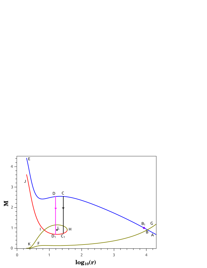
Figure 1: Phase topology corresponding to the multi-transonic shocked accretion and its associated wind branches obtained for a prograde flow characterized by $\left[{\cal E}=1.00001,\lambda=2.6,\gamma=1.43,a=0.215\right]$. The radial Mach number and the radial distance in logarithmic scale and in units of $GM_{BH}/c^{2}$ has been plotted along the abscissa and the ordinate, respectively. ABB₁CDE is the transonic accretion solution constructed through the saddle type outer critical point B (located at a distance $10815.150$ in units of $GM_{BH}/c^{2}$) and the corresponding outer sonic point B₁ (located at a distance $8437.850$ in units of $GM_{BH}/c^{2}$), FBG is the associated transonic self-wind solution passing through the outer critical point. The homoclinic orbit KIHC₁D₁IJ consists of the transonic accretion and its associated self-wind solutions passing through the saddle type inner critical point I (located at a distance $6.999$ in units of $GM_{BH}/c^{2}$). The corresponding inner sonic point (not shown in the figure) is located at a distance $5.985$ in units of $GM_{BH}/c^{2}$ measured from the horizon. The centre type middle critical point shown by an asterisk (*) and marked by L located at a distance $17.213$ in units of $GM_{BH}/c^{2}$. Among two formally obtained shock transitions CC₁ and DD₁, the shock formed between the outer sonic point and the middle critical point is found to be the stable one. ABB₁CC₁D₁IJ represents the actual multi-transonic accretion flow connecting infinity with the black hole event horizon and contains the integral solutions constructed through the outer and the inner sonic points, respectively.

In Figure 1 we plot one such flow topology for $\left[{\cal E}=1.00001,\lambda=2.6,\gamma=1.43,a=.215\right]$. The radial Mach number has been plotted along the the Y axis and the equatorial radial distance $r$ scaled in units of $GM_{BH}/c^{2}$, has been plotted along the X axis in logarithmic ($\log_{10}$) scale. Three regular critical points are obtained – the outermost saddle type critical point $r_{c}^{out}$ located at $r=10815.150$, the centre type middle critical point $r_{c}^{mid}$ located at $r=17.213$, and the saddle type innermost critical point $r_{c}^{in}$ formed at $r=6.999$. $\left[r_{c}^{out},r_{c}^{mid},r_{c}^{in}\right]$ are computed by numerically solving the algebraic equation obtained by substituting the value of $\left[u,c_{s}\right]_{\rm r_{c}}$ (as defined in equation 39) in eq. (34). The value of $u$ and $c_{s}$ at any one of the three different critical points $\left[r_{c}^{out},r_{c}^{mid},r_{c}^{in}\right]$ can now be calculated by substituting the respective values of the critical points back to the eq. (39). As already mentioned, Mach numbers can have different values computed at three different critical points. Hence $r_{c}^{out}$, $r_{c}^{mid}$, and $r_{c}^{in}$ are not collinear on $M-\log_{10}(r)$ phase plane. The space gradient of the advective velocity $\left(\mathrm{d}u/\mathrm{d}r\right)_{\rm r_{c}}$ is computed using eq. (42) and the space gradient for the polytropic sound speed is calculated by substituting the value of $\left(\mathrm{d}u/\mathrm{d}r\right)_{\rm r_{c}}$ into eq. (37) in the critical limit. We now use the initial values $\left[u,c_{s},\mathrm{d}u/\mathrm{d}r,\mathrm{d}c_{s}/\mathrm{d}r\right]_{\rm r_{c}^{out}}$ to integrate eq. (37) - (38) simultaneously to obtain the stationary transonic branch ABB₁DE on the $\left(M-log_{10}(r)\right)$ phase plane passing through the outermost saddle type critical point $r_{c}^{out}$ as denoted by B on the phase plane. Since a critical point and a sonic point does not form at same radial distance, AB is not the subsonic branch of the flow, nor does the segment BCDE represent the supersonic branch. The location of the sonic point is found by integrating $du/dr$ and $dc_{s}/dr$ simultaneously to compute the radial equatorial distance for which Mach number becomes exactly equals to unity. For $\left[{\cal E}=1.00001,\lambda=2.6,\gamma=1.43,a=0.215\right]$ used to obtain figure 1, we found the value of the outermost sonic point $r_{s}^{out}$ to be $8437.850$ which has been identified in the figure 1 as B₁. Hence ABB₁ represents the subsonic flow and B₁CDE represents the supersonic flow. We define $\Delta{r_{cs}}=\left(r_{c}-r_{s}\right)$ to be a measure of the difference of the location of the critical and the sonic points. Hence the line segment measured along the X axis and corresponding to BB₁ represents the logarithmic value of $\Delta{r_{cs}}^{out}$ for the particular values of the $\left[{\cal E},\lambda,\gamma,a\right]$used to obtain figure 1. One can study the dependence of $\Delta{r_{cs}}^{out}$ on $\left[{\cal E},\lambda,\gamma,a\right]$as well for the entire domain of the four parameters ${\cal E},\lambda,\gamma$ and $a$ to apprehend the effect of the black hole space time as well as the dynamical and the thermodynamic properties of the flow on the distinction between the sonic and the critical points. It is important to note that however small can $\Delta{r_{cs}}$ be made, it never vanishes for any value of $\left[{\cal E},\lambda,\gamma,a\right]$. This indicates that the non isomorphism of the critical and the sonic properties of the flow are not any artifact of the choice of the initial boundary conditions describing the stationary transonic accretion.

If the value of the ${\dot{M}}$ is also provided along with $\left[{\cal E},\lambda,\gamma,a\right]$, one can calculate the values of all possible thermodynamic quantities corresponding to the flow, the pressure $p$, the density $\rho$ and the ion temperature $T$ of the accreting fluid, for example, at all radial distances stating from the infinity upto a very close proximity of $r_{+}=1+\sqrt{1-a^{2}}$. The trans-critical solution passing through the outermost critical point $r_{c}^{out}$ seems to be doubly degenerate as is observed from the appearance of the phase topology FBG on the $M-\log_{10}(r)$ phase plane. FBG is obtained by integrating eq. (37 – 38) using $\left[u,c_{s},\mathrm{d}u/\mathrm{d}r,\mathrm{d}c_{s}/\mathrm{d}r\right]_{\rm r_{c}^{out}}$ but for the values of $\left(\mathrm{d}u/\mathrm{d}r\right)_{\rm r_{c}^{out}}$ corresponding to the negative sign in eq. (42). Such twofold degeneracy is the consequence of the $\pm{u}$ degeneracy appearing in the expression for the energy first integral of motion as defined in eq. (34). Such degeneracy has, however, been apparently removed by orienting the phase portrait so that each phase topology represents either the accretion or the wind. The wind branch FBG, obtained by the advective velocity reversal symmetry, is a mathematical counter part of the accretion flow and is usually termed as the ‘self -wind’. Had it been the situation that instead of starting from the infinity and heading toward the compact object, transcritical solution would generate from the close proximity of the accretor and would fly off from such object, FBG would denote the phase trajectory along which it would escape to infinity. The phrase ‘wind solution’ stems from the fact that the phase portrait corresponding to the solar wind solution due to [124] was topologically similar with the aforementioned mathematical counterpart of the accretion solution associated with the classical [125] flow.

A similar procedure may be used to obtain the transonic stationary accretion and the wind solutions passing through the innermost saddle type critical point $r_{c}^{in}$ which is located at a radial distance $r=6.999$ and is marked by I on the $M-log_{10}(r)$ phase plane. The corresponding value of the radial distance for the sonic point $r_{s}^{in}$ comes out to $r=5.985$.

The transcritical accretion solution HIJ constructed through the inner critical point $r_{c}^{in}$ folds back onto itself and joins with the corresponding transcritical self-wind branch HIK. The combined transcritical accretion-wind solution through the $r_{c}^{in}$ thus forms a homoclinic orbit on the $M-log_{10}(r)$ phase plane. Such a homoclinic phase trajectory encompasses the centre type critical point $r_{c}^{mid}$ flanked between $r_{c}^{out}$ and $r_{c}^{in}$. The point of inflection H of the homoclinic orbit is actually a ‘irregular’ and ‘singular’ critical point. A tangent drawn through such a point of inflection comes out to be parallel to the Y axis. The Mach number $M$ is defined at that point, whereas its space gradient $dM/dr$ is not. The advective velocity $u$ is continuous at that point but its space gradient diverges. At the point of inflection of the homoclinic orbit, the denominator of eq. (38) vanishes, allowing the corresponding numerator to assume a non-zero value. It is therefore understood that along with three regular critical points $\left[r_{c}^{out},r_{c}^{mid},r_{c}^{in}\right]$, multi-critical stationary flow solution always possesses one more critical point which is of singular type. The only exception observed for a very special case where the multi-critical flow consists of two heteroclinic orbits since no homoclinic orbit for such configuration can further be realized. The transcritical heteroclinic orbits on $M-log_{10}(r)$ phase plane is characterized by the identical value of the entropy accretion rate $\dot{\Xi}$ evaluated for the solution passing through the innermost saddle point $r_{c}^{in}$ as well as for the solution constructed through the outermost saddle point $r_{c}^{out}$.

A homoclinic orbit has its existence only in isolation and such a trajectory does not qualify as a global transcritical solution. Any realistic transcritical solution has to connect infinity with the event horizon to ensure the existence of the corresponding transonic flow. A local transcritical homoclinic integral flow solution can be made physically realizable by joining it with the transcritical non-homoclinic solution constructed through the outermost saddle type critical point $r_{c}^{out}$ through a discontinuous shock transition since for non-dissipative inviscid flow two different transonic solutions can not be smoothly connected to each other through any regular transition. In connection to astrophysical flows. such a statement translates to the fact that no regular smooth stationary transonic solution can encounter more than one sonic point, and a multi-transonic solution can only be realized when two different smooth transonic solutions can be connected through a stationary shock. The entropy accretion rate $\dot{\Xi}_{in}$ for the accretion solution HIJ is greater than the entropy accretion rate $\dot{\Xi}_{out}$ for the accretion solution AB₁CDE. Subjected to the appropriate perturbative environment, a standing shock which generates $\Delta{\dot{\Xi}}=\left(\dot{\Xi}_{in}-\dot{\Xi}_{out}\right)$, allows the flow solution through the outer sonic point to make a discontinuous transition onto its subsonic homoclinic counterpart, i.e., the subsonic part of the transonic accretion solution HIJ. The combined multi-transonic shocked accretion solution would thus be consists of a segment (both subsonic and supersonic) of ABB₁CDE and a segment (both subsonic and supersonic) of HIJ connected by a discontinuous shock, the location of which is to be determined by solving certain set of algebraic equations.

6.2 The relativistic shock of Rankine-Hugoniot type

In the present work, the first integrals of motion are the conserved specific energy and the mass accretion rate. For the non-dissipative inviscid accretion considered in our work, the shock produced is assumed to be of energy preserving Rankine Hugoniot [128, 129, 130, 131, 132] type. The corresponding shock thickness has to be negligibly small compared to any characteristic length scale of the flow so that no dissipation of energy as a consequence of the strong temperature gradient in between the inner and the outer boundaries of the shock is allowed, where the terms ‘inner’ and the ‘outer’ are referred with respect to the proximity to the black hole event horizon.

For a neutral ideal fluid, the general relativistic shock condition has been discussed by several authors [133, 134, 135, 136, 137, 138]. In connection to rotating axisymmetric accretion in the Kerr metric, the general relativistic Rankine Hugoniot condition can be expressed as [117, 104]

$$\left[\left[{\rho}u\Gamma_{u}\right]\right]=0\,,$$

$$\left[\left[{\large\sf T}_{t\mu}{\eta}^{\mu}\right]\right]=\left[\left[(p+\epsilon)v_{t}u\Gamma_{u}\right]\right]=0\,,$$

$$\left[\left[{\large\sf T}_{\mu\nu}{\eta}^{\mu}{\eta}^{\nu}\right]\right]=\left[\left[(p+\epsilon)u^{2}\Gamma_{u}^{2}+p\right]\right]=0\,,$$ (43)

where $\Gamma_{u}=1/\sqrt{1-u^{2}}$ is the Lorentz factor and $T_{\mu\nu}$ is the corresponding energy momentum tensor. In the above equation, $\left[\left[f\right]\right]$ denotes the discontinuity of any relevant physical quantity $f$ across the surface of discontinuity, i.e., $\left[\left[f\right]\right]=f_{2}-f_{1}$, where $f_{1}$ and $f_{2}$ are the boundary values of the quantity $f$ on the two sides of such surface.

Simultaneous solution of Eq. (43) yields the shock invariant quantity for stationary axisymmetric accretion in hydrostatic equilibrium in vertical direction which changes continuously only across the shock surface. We obtain an analytical expression for such a shock invariant quantity in terms of various local accretion variables and in terms of various initial boundary conditions describing the flow. During the numerical integration of the flow equations along the transonic solution ABB₁CDE, we calculate the shock invariant. Simultaneously we calculate the same invariant while integrating the flow equations along the solution JIH starting from the inner sonic point up to the irregular sonic point on the homoclinic orbit (the point of inflection). We then determine the radial distance $r_{sh}$ where the numerical values of the shock invariant quantity is evaluated by integrating the two different flow segments as described above become identical. For every $\left[{\cal E},\lambda,\gamma,a\right]$  allowing the formation of a stationary shock, one in general obtains two different values of $r_{sh}$. Out of the two formal shock locations, the inner one (with reference to the proximity of $r_{+}$) is always located in between the innermost and the middle sonic point, whereas the outer shock location is obtained in between the middle and the outermost sonic point. The shock strength $M_{-}/M_{+}$ is different for these two shocks. Following the standard stability analysis procedure as provided in [97], one finds that the outer shock location is stable. Hereafter, we will refer to the stable outer shock location whenever we use the word shock, and all shock related calculations will exclusively be performed with respect to that outer stable shock.

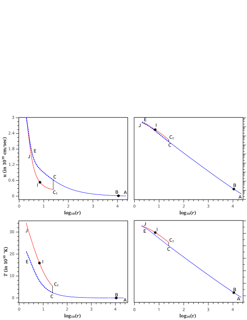
Figure 2: Variation of the advective flow velocity $u$ (upper left panel), rest mass density $\rho$ (upper right panel), flow ion temperature $T$ (lower left panel) and pressure (lower right panel) corresponding to the flow topology presented in the figure 1 and for a black hole with mass ${\rm 3.6}\times{\rm 10}^{\rm 6}M_{\odot}$ and associated accretion rate ${\dot{M}}=4.29\times{\rm 10}^{\rm-6}M_{\odot}{\rm Yr^{-1}}$. The solid vertical line in each panel represents the shock transition and the labeling alphabets are in one to one correspondence with those used in figure 1, see text for further detail.

ABB₁CC₁IJ on the $M-\log_{10}(r)$ phase plane represents the combined multi-transonic shocked flow as shown in figure 1. We need to calculate the values of various accretion variables along this segment of the flow topology. A sudden discontinuous transition for all such variables at the shock location is to be accounted for. We define the ‘pre-shock variables’ to be the value of any accretion variable at the shock location evaluated at the point C, and denote all such variables by a subscript ‘-’. Similarly, a ‘post shock variable’ is defined to be the value of the same variable (for same $\left[{\cal E},\lambda,\gamma,a\right]$  as implied) evaluated at the point C₁ and is denoted using a subscript ‘+’. The ratio of the pre (post) to the post (pre) shock variable for a set of fixed value of $\left[{\cal E},\lambda,\gamma,a\right]$  will provide the measure of the discontinuous change of such variables due to the presence of the shock. Had it been the situation that the shock would not form, and the flow would uninterruptedly follow ABB₁CDE to approach the event horizon, the flow variables would change continuously and no abrupt considerable alteration of the flow variables would be realized. Since a sudden change of the value of a flow variable is associated with the formation of a stationary shock in our model, a careful study of the radial profile of any accretion variable would provide a conclusive information about the appearance of a stationary shock. The radial variation of certain accretion variables (density, velocity, ion temperature etc.) are required to construct the observed spectra emergent from the accreting black hole, and the presence of shock can thus be inferred by investigating such spectral profile.

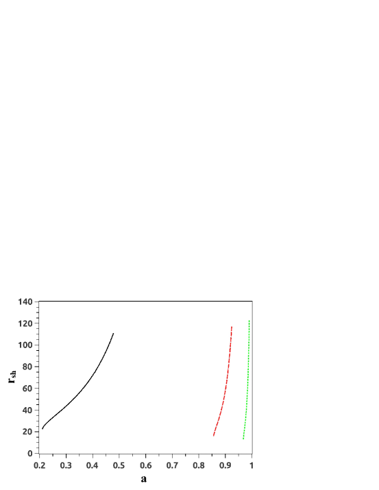
Figure 3: Variation of the shock location $r_{sh}$ (plotted along the ordinate) with the Kerr parameter $a$ (plotted along the abscissa) for the prograde accretion characterized by $\left[{\cal E}=1.00001,\gamma=1.43\right]$ for three different values of the specific angular momentum $\lambda=2.6$ (solid black line at left), $\lambda=2.17$ (long dashed red line at the middle) and $\lambda=2.01$ (short dashed green line at the right). The shock location non-linearly correlates with the black hole spin.

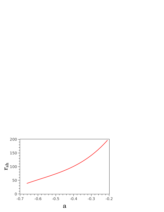
Figure 4: Variation of of the shock location $r_{sh}$ (plotted along the ordinate) with the Kerr parameter $a$ (plotted along the abscissa) for the retrograde accretion characterized by $\left[{\cal E}=1.00001,\lambda=3.3,\gamma=1.4\right]$.

6.3 Shock induced discontinuous transition of flow variables

In Figure 2, we show the variation of the advective velocity $u$ scaled in units of $10^{10}$ cm/sec, the bulk ion temperature $T$ scaled in units of $10^{10}$ degree Kelvin, flow density $\rho$ in gm/cc and fluid pressure $p$ in dyne/cm², for a black hole with mass $M_{BH}={\rm 3.6}\times{\rm 10}^{\rm 6}M_{\odot}$ and accretion rate ${\dot{M}}=4.29\times{\rm 10}^{\rm-6}M_{\odot}{\rm Yr^{-1}}$. $\left[{\cal E}=1.00001,\lambda=2.6,\gamma=1.43,a=0.215\right]$ has been used as four initial boundary conditions to set up the flow. B and I are the outermost and the innermost saddle type critical points, respectively. CC₁ indicates the stable standing shock transition. ABCE indicates the variation of the respective accretion variables along the transonic solution passing through the outer sonic point. If the shock would not form, the value of the respective variables would change continuously and monotonically, and the space evolution of such variables would be presented by the line segment ABCE. One could integrate the flow equations along the solutions passing through the outer sonic point upto the very close proximity of the event horizon and can obtain the value of the respective variable on ABCE in the extremely close vicinity of the black hole event horizon for a shock free solution. If, however, the shock forms, there will be an abrupt discontinuous change of the value of the respective variable and its $r$ variation profile can actually be demonstrated by the combined segment ABCC₁IJ. Once again, one can integrate the set of differential and the algebraic equations governing the flow upto the very close proximity of $r_{+}$ and the corresponding value of the respective variable at a radial distance nearly equal to $r_{+}$ can be obtained for a shocked multi-transonic integral solution.

7 Dependence of the shock location and the shock related quantities on $\left[{\cal E},\lambda,\gamma,a\right]$

In this section we study the dependence of the shock location $r_{sh}$ and various pre and post shock values of the accretion variables on $\left[{\cal E},\lambda,\gamma,a\right]$. To study such dependence on any particular parameter of the set $\left[{\cal E},\lambda,\gamma,a\right]$, on specific flow energy ${\cal E}$ for example, other three parameters $\lambda,\gamma$ and $a$ are to be kept constant for the entire range of ${\cal E}$ for which such dependence is studied. Whereas a wide range of choice for $\left[{\cal E},\lambda,\gamma,a\right]$ is available to produce a mono-transonic accretion, only a limited non linear region of $\left[{\cal E},\lambda,\gamma,a\right]$  allows the existence of a shocked multi-transonic flow. A continuous range of all $\left[{\cal E},\lambda,\gamma,a\right]$  can not be used to construct such flow configuration since the Rankine Hugoniot condition is satisfied only for a small range of $\left[{\cal E},\lambda,\gamma,a\right]_{\rm mcas}{\in}\left[{\cal E},\lambda,\gamma,a\right]_{\rm mca}$, where ‘mcas’ stands for ‘multi-critical accretion with shock’ and ‘mca’ indicates the ‘multi-critical accretion’ in general. $\left[{\cal E},\lambda,\gamma,a\right]{\subset}\left[{\cal E},\lambda,\gamma,a\right]_{\rm mcas}$ thus provides a true stationary multi-transonic accretion. We thus use various ‘patches’ of the region $\left[{\cal E},\lambda,\gamma,a\right]_{\rm mcas}$ to study the dependence of the shock related entities on $\left[{\cal E},\lambda,\gamma,a\right]$.

One understands that such a choice of $\left[{\cal E},\lambda,\gamma,a\right]$  will indeed provide the generic profile for the aforementioned dependence. Consider a set of fixed values $\left[\lambda_{1},\gamma_{1},a_{1}\right]$ to study the dependence of, say, the shock location $r_{sh}$ on the available (for which the shock forms, subjected to the fixed set $\left[\lambda_{1},\gamma_{1},a_{1}\right]$) range of the specific energy starting from ${\cal E}_{min}$ to ${\cal E}_{max}$. Such $`r_{sh}-{\cal E}^{\prime}$ profile can also be explored for any other fixed set, say $\left[\lambda_{2},\gamma_{2},a_{2}\right]$ for which the Rankine Hugoniot condition gets satisfied, only with the obvious difference that the numerical values corresponding to ${\cal E}_{min}$ and ${\cal E}_{max}$ associated with the flow described by $\left[\lambda_{2},\gamma_{2},a_{2}\right]$ will be different as compared to the values of ${\cal E}_{min}$ and ${\cal E}_{max}$ corresponding to the initial boundary conditions defined by $\left[\lambda_{1},\gamma_{1},a_{1}\right]$. Hence for any set of values $\left[\lambda,\gamma,a\right]$ for which the shock forms, the dependence of $r_{sh}$ on ${\cal E}$ can be studied. Similarly, the dependence of any shock related entity on any one of the initial boundary conditions $\left[{\cal E},\lambda,\gamma,a\right]$  can be studied for a fixed set of values of the rest of the initial boundary conditions for which a shocked multi-transonic accretion configuration can be realized.

We observe that the shock location correlates with the specific angular momentum $\lambda$ and anti-correlates with the specific energy ${\cal E}$ and the polytropic index $\gamma$. Such trends are independent of the black hole spin parameter, and hence remain the same for the maximally rotating Kerr as well as for a non-rotating Schwarzschild black hole. The aforementioned dependence does not explicitly provide any information about the dependence of the shock related quantities on the nature of the space time metric. In this work, we are, however, mainly interested to study how the properties of the post shock flow at the close proximity of the event horizon are influenced by the spin parameter of the astrophysical black holes. Since that spin parameter determines the spacetime metric, our motivation is to study how the properties of the transonic black hole accretion are determined by the nature of the black hole metric. In the subsequent sections we study the dependence of the shock location as well as other shock related properties on the Kerr parameter in greater detail.

7.1 Dependence of the shock location on black hole spin

The characteristic features of the shocked accretion for the entire range of the Kerr parameter, for the prograde as well as for the retrograde flow, can not be studied for any single fixed set $\left[{\cal E},\lambda,\gamma\right]$. No such fixed set is available for which the Rankine Hugoniot conditions are satisfied for the entire range of the Kerr parameters for the prograde ($\left[0{\geq}a{\geq}1\right]$), as well as for the retrograde ($\left[-1{\geq}a{\geq}0\right]$) flow, respectively. This can easily be shown by plotting the region $\left[{\cal E},\lambda,\gamma,a\right]_{\rm mca}$ embedded in the entire four dimensional hypersurface $\left[{\cal E},\lambda,\gamma,a\right]{\supset}\left[{\cal E},\lambda,\gamma,a\right]_{\rm mca}$ to ensure that no single value of $\left[{\cal E},\lambda,\gamma\right]$ is available for which even a multi-critical solution, let alone a multi-transonic shocked solution, exists for (-1${\leq}a{\leq}$1). We have chosen three different representative sets $\left[{\cal E}=1.00001,\lambda=2.6,\gamma=1.43\right],\left[{\cal E}=1.00001,\lambda=2.17,\gamma=1.43\right]$ and $\left[{\cal E}=1.00001,\lambda=2.01,\gamma=1.43\right]$ to cover a significant range of the low to moderately high ($0.2{\lower 2.15277pt\hbox{$\;\buildrel<\over{\sim}\;$}}a{\lower 2.15277pt\hbox{$\;\buildrel<\over{\sim}\;$}}0.5$), high ($0.85{\lower 2.15277pt\hbox{$\;\buildrel<\over{\sim}\;$}}a{\lower 2.15277pt\hbox{$\;\buildrel<\over{\sim}\;$}}0.925$), and very high ($0.9655{\lower 2.15277pt\hbox{$\;\buildrel<\over{\sim}\;$}}a{\lower 2.15277pt\hbox{$\;\buildrel<\over{\sim}\;$}}0.99$) values of the black hole spin, respectively, to study the dependence of $r_{sh}$ on the black hole spin for prograde flow. Such values of $\left[{\cal E},\lambda,\gamma\right]$ are chosen to maximize the available range of the Kerr parameter (for which the shock forms) for three different spans of the black hole spin mentioned above. This is to avail such range by minimally varying the initial configuration. For three different ranges, only the specific angular momentum $\lambda$, that too by a rather small amount, has been varied for each set of initial $\left[{\cal E},\lambda,\gamma\right]$, by keeping the subset $\left[{\cal E},\gamma\right]$ at its fixed value.

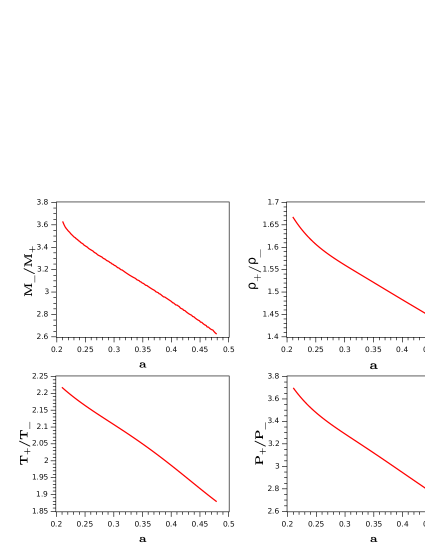
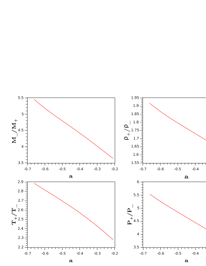
Figure 5: Variation of the shock strength (upper left panel), the shock compression ration (upper right panel), the ratio of the post to the pre shock temperature (lower left panel) and the ratio of the post to the pre shock pressure (lower right panel) with the Kerr parameter $a$ (for each panel plotted along the abscissa) for the prograde flow characterized by $\left[{\cal E}=1.00001,\lambda=2.6,\gamma=1.43\right]$.

Figure 6: Variation of the shock strength (upper left panel), the shock compression ration (upper right panel), the ratio of the post to the pre shock temperature (lower left panel) and the ratio of the post to the pre shock pressure (lower right panel) with the Kerr parameter $a$ (for each panel plotted along the abscissa) for the retrograde flow characterized by $\left[{\cal E}=1.00001,\lambda=3.3,\gamma=1.4\right]$.

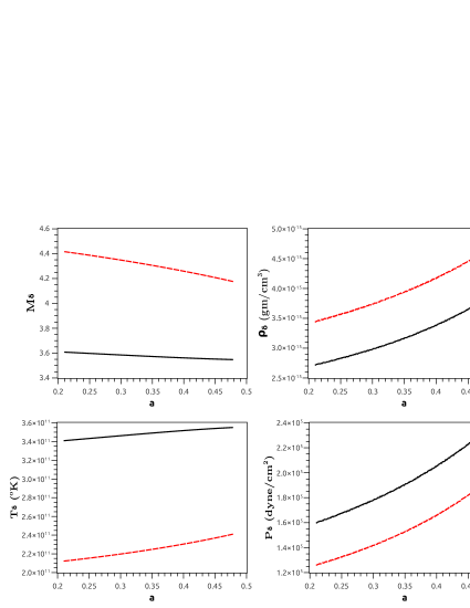
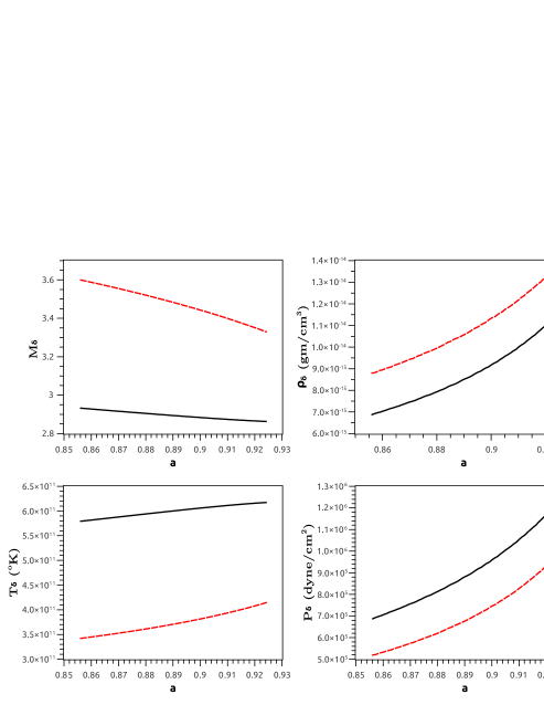
Figure 7: Variation of the quasi-terminal Mach number (upper left panel), quasi-terminal density (upper right panel), quasi-terminal temperature (lower left panel) and the quasi-terminal pressure (lower left panel) with the Kerr parameter $a$ (plotted along the abscissa) for shocked (dashed red line) and for the hypothetical shock free (solid black line) prograde flow characterized by $\left[{\cal E}=1.00001,\lambda=2.6,\gamma=1.43\right]$.

Figure 8: Variation of the quasi-terminal Mach number (upper left panel), quasi-terminal density (upper right panel), quasi-terminal temperature (lower left panel) and the quasi-terminal pressure (lower left panel) with the Kerr parameter $a$ (plotted along the abscissa) for shocked (dashed red line) and for the hypothetical shock free (solid black line) prograde flow characterized by $\left[{\cal E}=1.00001,\lambda=2.17,\gamma=1.43\right]$.

As a representative value, we take $\left[{\cal E}=1.00001,\lambda=3.3,\gamma=1.4\right]$ to cover a reasonably large range of the black hole spin for which the shocked multi-transonic accretion solution can be constructed for the retrograde flow. In Figure 3, we plot the shock location $r_{sh}$ as a function of the Kerr parameter $a$ for there prograde flow with fixed set of $\left[{\cal E}=1.00001,\gamma=1.43\right]$ and for three different values of $\lambda$ (as shown in the figure) for three different ranges of the Kerr parameters (as mentioned in the figure) for which the multi-transonic shocked solutions can be constructed. We observe that the shock location non-linearly correlates with the black hole spin for the prograde flow. We infer that for similar initial conditions describing the flow, the shock forms closest to the event horizon for a Schwarzschild type black hole, and furthest from the event horizon for an extremal rotating Kerr black hole. We find the same $`r_{sh}-a^{\prime}$ profile for the retrograde flow as well. In Figure 4 the shock location is plotted against the black hole spin for the retrograde flow characterized by $\left[{\cal E}=1.00001,\lambda=3.3,\gamma=1.4\right]$.

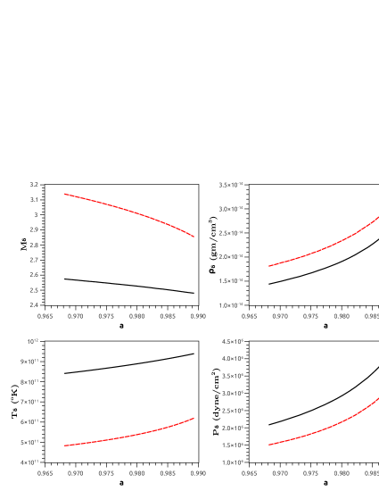
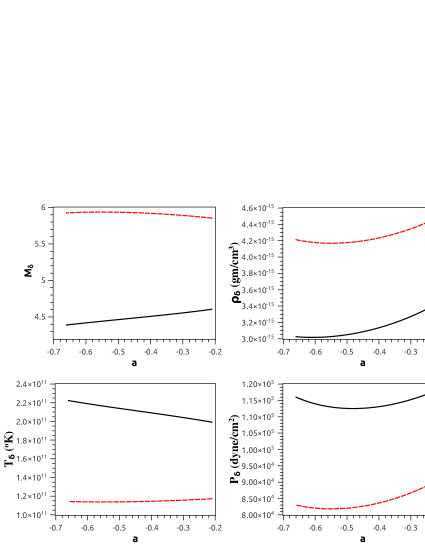
Figure 9: Variation of the quasi-terminal Mach number (upper left panel), quasi-terminal density (upper right panel), quasi-terminal temperature (lower left panel) and the quasi-terminal pressure (lower left panel) with the Kerr parameter $a$ (plotted along the abscissa) for shocked (dashed red line) and for the hypothetical shock free (solid black line) prograde flow characterized by $\left[{\cal E}=1.00001,\lambda=2.01,\gamma=1.43\right]$.

Figure 10: Variation of the quasi-terminal Mach number (upper left panel), quasi-terminal density (upper right panel), quasi-terminal temperature (lower left panel) and the quasi-terminal pressure (lower left panel) with the Kerr parameter $a$ (plotted along the abscissa) for shocked (dashed red line) and for the hypothetical shock free (solid black line) retrograde flow characterized by $\left[{\cal E}=1.00001,\lambda=3.3,\gamma=1.4\right]$.

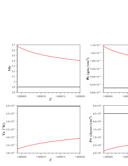
Figure 11: Variation of the quasi-terminal Mach number (upper left panel), quasi-terminal density (upper right panel), quasi-terminal temperature (lower left panel) and the quasi-terminal pressure (lower left panel) with the specific flow energy ${\cal E}$ (plotted along the abscissa) for shocked (dashed red line) and for the hypothetical shock free (solid black line) prograde flow characterized by $\left[\lambda=2.17,\gamma=1.43,a=0.881049812\right]$.

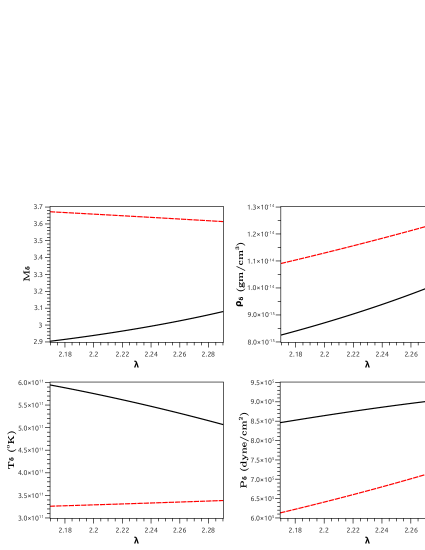
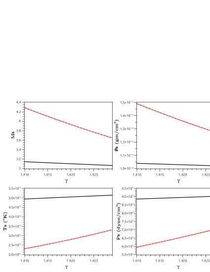
Figure 12: Variation of the quasi-terminal Mach number (upper left panel), quasi-terminal density (upper right panel), quasi-terminal temperature (lower left panel) and the quasi-terminal pressure (lower left panel) with the specific flow angular momentum $\lambda$ (plotted along the abscissa) for shocked (dashed red line) and for the hypothetical shock free (solid black line) prograde flow characterized by $\left[{\cal E}=1.000004,\gamma=1.43,a=0.881049812\right]$.

Figure 13: Variation of the quasi-terminal Mach number (upper left panel), quasi-terminal density (upper right panel), quasi-terminal temperature (lower left panel) and the quasi-terminal pressure (lower left panel) with the adiabatic index $\gamma$ (plotted along the abscissa) for shocked (dashed red line) and for the hypothetical shock free (solid black line) prograde flow characterized by $\left[{\cal E}=E=1.000004,\lambda=2.28,a=0.881049812\right]$.

7.2 Dependence of shock induced flow variables on black hole spin

We would like to study how the characteristic dynamical and the thermodynamic features of the post shock flow are influenced by the black hole spin. One way of looking at this problem is to study the ratio of the pre (post) to the post (pre) shock values of various accretion variables. Such a ratio serves as a marker of how the presence of a stationary shock introduces a sudden change in the value of the flow variables which in turn make a observable difference in the characteristic black hole spectra. For any flow variable $f$, $f_{-}$ denotes its pre shock value evaluated at the shock location on the transonic solution passing through the outer sonic point and $f_{+}$ denotes its post shock value evaluated at the shock location on the transonic solution constructed through the inner sonic point. For prograde flow characterized by $\left[{\cal E}=1.00001,\lambda=2.6,\gamma=1.43\right]$, in figure 6 we plot the ratio of the pre to the post shock Mach number ($M_{-}/M_{+}$), and post to the pre shock flow temperature ($T_{+}/T_{-}$), density ($\rho_{+}/\rho_{-}$) and pressure ($p_{+}/p_{-}$), respectively. ($M_{-}/M_{+}$) is termed as the shock strength as mentioned earlier and ($\rho_{+}/\rho_{-}$) is termed as the shock compression ratio. The shock strength anti-correlates with the shock location. The closer the shock forms to the event horizon, the higher the gravitational potential energy liberated resulting the formation of a stronger shock. A strong shock also compresses the flow by a considerable amount. As a result (since the shock as well as the flow under consideration is assumed to be energy preserving) the temperature and the pressure of the flow also increases. Thus $\left[\left(\rho_{+}/\rho_{-}\right),\left(T_{+}/T_{-}\right),\left(p_{+}/p_{-}\right)\right]$ anti-correlates with the shock location and hence with the black hole spin angular momentum (the Kerr parameter $a$).

Identical trends are observed for two other ranges of the black hole spin parameters explored (characterized by $\left[{\cal E}=1.00001,\lambda=2.17,\gamma\right.$$\left.=1.43\right]$ and $\left[{\cal E}=1.00001,\lambda=2.01,\gamma=1.43\right]$) in this work for the prograde flow, as well as for the retrograde flow characterized by $\left[{\cal E}=1.00001,\right.$ $\left.\lambda=3.3,\gamma=1.4\right]$. Such $`\left[\left(M_{-}/M_{+}\right),\left(\rho_{-}/\rho_{+}\right),\left(T_{+}/T_{-}\right),\left(p_{+}/p_{-}\right)\right]-a^{\prime}$ variation for the retrograde flow has been represented in figure 6. We observe weakly rotating (low $\lambda$), hot (high ${\cal E}$), purely non relativistic (high $\gamma$) flow to form the strongest shock (the shock forms closest to the event horizon) for black hole with any value of the intrinsic spin angular momentum, i.e., the Kerr parameter $a$, and accretion onto a Schwarzschild black hole undergoes a strong shock transition compared to the case when matter with the same dynamical and thermodynamic properties accretes onto a Kerr hole. This summarizes how the shock formation phenomena and the properties of a multi-transonic flow get influenced by the space time metric (characterized by $a$), the dynamical (characterized by $\left[{\cal E},\lambda\right]$) and the thermodynamic (characterized by $\gamma$) properties of the accreting material.

As mentioned earlier, in this work we did not consider viscous transport of angular momentum, rather the specific angular momentum has been parameterized by astrophysically relevant constant numbers. Owing to the fact that the accretion flow considered in this work has small amount of rotational energy and considerable advective velocity, the infall time scale is much smaller than the viscous time scale and inviscid flow assumption is not unjustified - especially for the supersonic part of the flow. For viscous accretion, specific energy would not be a first integral of motion, and the differential equation for the conservation of angular momentum would also to be taken into account. That clearly is beyond the scope of the present work. However, one can intuitively predict the possible modifications incurred by the inclusion of the viscous effects in the results obtained using our simple inviscid flow model.

One of the significant effects of the viscosity is to reduce the local value of the specific angular momentum at every radial distance of a stationary axisymmetric flow. It is found that the location of the sonic points anti-correlates with the specific flow angular momentum $\lambda$. Weakly rotating flow produces the steeper value of the space gradient of the advective velocity. This indicates that the introduction of viscosity (reduction of the local angular momentum at any representative radial distance) the transonic surfaces will be pushed further out, and consequently associated shock locations would also change, for the same set of initial boundary conditions.

Construction of the full space time dependent viscous shock solutions in the Kerr metric, even using fully numerical scheme, is far from reality at this moment as we believe. Even forty years after the discovery of the [139] $\alpha$ prescription, exact modelling of viscous flow by explicitly incorporating appropriate dissipative mechanics is still a recalcitrant task to accomplish even for a purely Newtonian flow, let alone for general relativistic accretion in the Kerr space time. Any immediate comparison of our present work with existing simulation results (related to the viscous shocked black hole accretion) does not seem to be possible at this stage as we believe.

8 The influence of black hole spin on quasi-terminal values

In this work, the numerical value of any accretion variable $V$ evaluated at a very close proximity $r_{\delta}=r_{+}+\delta$ ($r_{+}=1+\sqrt{1-a^{2}}$, and $\delta$ being a small number lying within the open interval $0<\delta<<1$) of the event horizon is dubbed as the corresponding ‘quasi terminal value’ of $V$, and is distinguished by a subscript $\delta$. The quasi-terminal value $V_{\delta}$ is computed by integrating the flow equations (along the stationary transonic branch) from the critical point $r_{c}$ down to $r_{\delta}$. We take $\delta=0.001GM_{BH}/c^{2}$ and perform our calculation for $V_{\delta}$ for a $3\times 10^{6}{M_{\odot}}$ black hole accreting at a rate of $4.29\times 10_{-6}{M_{\odot}}{\rm Yr}^{-1}$. Such values of $M_{BH}$ and ${\dot{M}}$ corresponds to our Galactic centre black hole and its environment where low angular momentum inviscid advective accretion model is considered as an appropriate approximation [see, e.g., 63, and references therein]. $M_{BH}$ and ${\dot{M}}$ used in this work are two representative values, and any other value for the black hole mass as well as for the accretion rate can be considered for our calculation of $V_{\delta}$.

For any generic flow variable $V$ we calculate the corresponding $V_{\delta}$ along two branches, either along the solution ABB₁CC₁IJ (see figure 1 and figure 2) for a multi-transonic shocked accretion flow, or for a hypothetical shock free solution ABB₁CDE passing through the outer sonic point only. For the same set of initial boundary condition $\left[{\cal E},\lambda,\gamma,a\right]$, the dependence $V_{\delta}^{shock}$ and $V_{\delta}^{no~{}shock}$ on the black hole spin angular momentum as well as on $\left[{\cal E},\lambda,\gamma\right]$ can be studied to estimate the impact of the shock formation phenomena in determining the properties of the matter extremely close to the black hole. This in turn helps to infer the influence of the shock formation on the observable spectra generated by the photon flux emanating out from the region inside the ISCO.

For co-rotating flow, in Figure 8 we plot the variation of the quasi-terminal values of the Mach number ($M_{\delta}$, the top left panel), flow density ($\rho_{\delta}$ in CGS units, top right corner), bulk ion temperature ($T_{\delta}$, in units of degree Kelvin, bottom left panel) and pressure ($p_{\delta}$ in CGS unit, bottom right panel) respectively, for both shocked solution (solid red line) and for the shock free solution (dashed blue line) on the black hole spin for multi-transonic flow characterized by $\left[{\cal E}=1.00001,\lambda=2.6,\gamma=1.43\right]$. Similar dependence is shown in figure 8 and figure 10 for other ranges of the Kerr parameter for which multi-transonic shocked flow can be described by $\left[{\cal E}=1.00001,\lambda=2.17,\gamma=1.43\right]$ and $\left[{\cal E}=1.00001,\lambda=2.01,\gamma=1.43\right]$, respectively. For the same set of $\left[{\cal E},\lambda,\gamma,a\right]$, we find that $M_{\delta}^{shock}<M_{\delta}^{no~{}shock}$ and $\rho_{\delta}^{shock}<\rho_{\delta}^{no~{}shock}$, whereas $T_{\delta}^{shock}>T_{\delta}^{no~{}shock}$ and $p_{\delta}^{shock}>p_{\delta}^{no~{}shock}$.

From Figure 1, one observes that for any $r<r_{s}^{in}$, the value of Mach number evaluated along the transonic solution passing through the outer sonic point is always greater than that evaluated on the transonic solution passing through the inner sonic point. At the shock, the Mach number decreases discontinuously, and although the value of the Mach number shoots up at a very high rate (the space gradient of the Mach number, i.e., $dM/dr$, becomes large), the Mach number for the supersonic flow in the post shock region can never exceed the value of the Mach number associated with the supersonic segment of the shock free solution at any $r$ since in that case the post shock supersonic flow would have to intersect the shock free supersonic solution on $`M-log_{10}(r)^{\prime}$ plane. Such a crossover is not allowed since no two phase topologies can intersect on a phase plane. Hence what actually one observes is $\left(dM/dr\right)^{shock}>\left(dM/dr\right)^{no~{}shock}$ but the trend $M_{\delta}^{shock}<M_{\delta}^{no~{}shock}$ is maintained. At the extreme close proximity of the event horizon ($r_{\delta}<<0.001$) the post shock supersonic branch asymptotically approaches the shock free supersonic branch, hence $M_{\delta}^{shock}{\longrightarrow}M_{\delta}^{no~{}shock}$ for such an extremely small value of $r_{\delta}$. Nevertheless, the criteria $M_{\delta}^{shock}-M_{\delta}^{no~{}shock}{\neq}0$ remains valid for for all values of $r_{\delta}$, however small $r_{\delta}$ can be made.

A similar situation is observed for the variation of $\rho_{\delta}$ with the spin as well. Although the density increases at the shock, close to $r_{+}$ the flow density corresponding to the shocked flow makes a crossover with the density profile corresponding to the shock free transonic flow, and starts decreasing gradually as has been observed in figure 2. For the flow temperature and pressure, no such crossover takes place and hence the trends $T_{\delta}^{shock}>T_{\delta}^{no~{}shock}$ and $p_{\delta}^{shock}>p_{\delta}^{no~{}shock}$ are uniformly maintained, see, e.g., Figure 2. Similar $`\left[M_{\delta},\rho_{\delta},T_{\delta},p_{\delta}\right]-a^{\prime}$ profiles are observed for the retrograde flow as well, see, e.g., Figure 10 for such variations for the counter-rotating accretion.

8.1 Dependence of quasi-terminal values on $\left[{\cal E},\lambda,\gamma\right]$

We also study the dependence of the quasi-terminal values on the specific energy ${\cal E}$ (figure 11), specific angular momentum $\lambda$ (figure 13), and the flow adiabatic index $\gamma$ (figure 13). For all such cases the following trend is found

$$M_{\delta}^{shock}<M_{\delta}^{no~{}shock},\rho_{\delta}^{shock}<\rho_{\delta}^{no~{}shock},T_{\delta}^{shock}>T_{\delta}^{no~{}shock},p_{\delta}^{shock}>p_{\delta}^{no~{}shock}$$ (44)

as has been observed for the black hole spin dependence of $\left[M_{\delta},\rho_{\delta},T_{\delta},p_{\delta}\right]$.

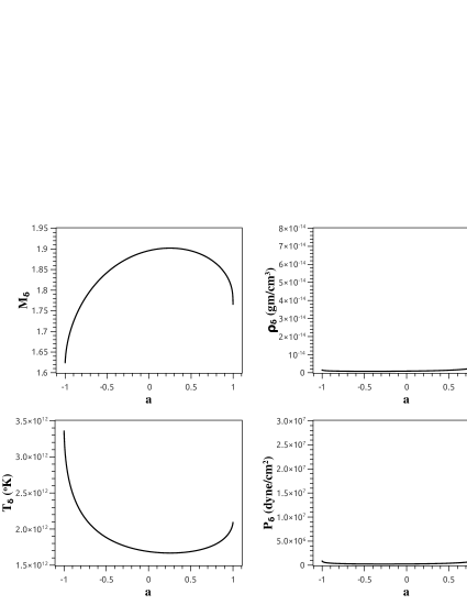
Figure 14: Variation of the quasi-terminal Mach number (upper left panel), quasi-terminal density (upper right panel), quasi-terminal temperature (lower left panel) and the quasi-terminal pressure (lower left panel) with Kerr parameter $a$ (plotted along the abscissa) for mono-transonic flow characterized by $\left[{\cal E}=1.2,\lambda=2.0,\gamma=1.6\right]$. The entire range of the Kerr parameter for both the prograde as well as the retrograde flow has been taken care of. The prograde and the retrograde branches are not symmetric.

In this work our prime motivation was to explicitly demonstrate how the black hole spin influences the properties of accreting matter sufficiently close to the horizon – mainly for shocked multi-transonic accretion flow – but also for shock free mono-transonic stationary accretion solutions as well, to provide a holistic approach. A limited part of $\left[{\cal E},\lambda,\gamma,a\right]\in\left[1{\lower 2.15277pt\hbox{$\;\buildrel<\over{\sim}\;$}}{\cal E}{\lower 2.15277pt\hbox{$\;\buildrel<\over{\sim}\;$}}2,0<\lambda{\leq}4,\right.$ $\left.4/3{\leq}\gamma{\leq}5/3,-1{\leq}a{\leq}1\right]$ forms shock. The choice of $\left[{\cal E},\lambda,\gamma\right]$ for which the spin dependence of multi-transonic stationary flow can be studied is constrained by the fact that the general relativistic Rankine Hugoniot conditions, as presented in eq. (43), are to be satisfied for the aforementioned set of $\left[{\cal E},\lambda,\gamma,a\right]$. To study the spin dependence one needs to have an appropriate combination of the Kerr parameter $a$ (the span of $a$ for which the dependence is to be examined) with $\left[{\cal E},\lambda,\gamma\right]$.

It is to be understood that along with $\left[{\cal E},\lambda,\gamma,a\right]$, one has to specify the mass of the black hole ${\rm M}_{\rm BH}$ and the corresponding accretion rate ${\dot{\rm M}}$ as well to evaluate the quasi-terminal pressure and density. Appropriate choice of $\left[{\rm M}_{\rm BH},{\dot{\rm M}}\right]$ was selected from the values corresponding to the Galactic centre black hole. If one would like to study the spectral signature of the black hole spin for a particular astrophysical candidate, one has to specify/find from the observational data, the values of $\left[{\cal E},\lambda,\gamma,a,{\rm M}_{\rm BH},{\dot{\rm M}}\right]$. For accretion flow in a pseudo-Schwarzschild space time, such values has been estimated for SgrA* [63, 140, 141].

For complete general relativistic flow in the Kerr metric, $\left[{\cal E}{\sim}1.000004,\lambda{\sim}2.16,\gamma{\sim}1.6,{\rm M}_{\rm BH}{\sim}\right.$ $\left.3\times 10^{6}{M_{\odot}},{\dot{\rm M}}{\sim}4.29\times 10_{-6}{M_{\odot}}{\rm Yr}^{-1}\right]$ can be used, which is in accordance with the relevant observational values corresponding to the Galactic centre black hole, see, e.g., [63, 140] and references therein.

The value of black hole spin for which shock forms for the above mentioned accretion parameters can be determined. Shock related dynamical and thermodynamic variables can then be estimated to reproduce the observed spectra of SgrA*. In this way it will be possible to predict the value of the black hole spin of a particular astrophysical candidate if the initial boundary conditions determining the accretion flow are observationally known a priory. This, however, requires a detail formalism capable of constructing the spectra using our dynamical model presented in this paper. Such calculations are, however, considerably involved, and are beyond the scope of this work.

9 Spin dependence of quasi-terminal values for the stationary mono-transonic accretion

It is instructive to investigate whether the characteristic feature of the black hole spin dependence of the quasi-terminal values remain invariant for a direct spin flip of the astrophysical black hole. In other words, we would like to understand whether the $`\left[M_{\delta},\rho_{\delta},T_{\delta},p_{\delta}\right]-a^{\prime}$ profile gets significantly altered when the initial boundary conditions are switched from $\left[{\cal E},\lambda,\gamma,a\right]$to $\left[{\cal E},\lambda,\gamma,-a\right]$. One understands that such exercise can not be performed for the multi-transonic accretion since the Rankine-Hugoniot conditions can not be satisfied for a certain $\left[{\cal E},\lambda,\gamma,a\right]$as well as for the same (magnitude wise) values of the $\left[{\cal E},\lambda,\gamma\right]$ and $a$ but with the oppositely signed value of $a$, i.e., for $\left[{\cal E},\lambda,\gamma,-a\right]$. This is a consequence of the fact that $\left[{\cal E},\lambda,\gamma,a\right]_{\rm mcas}$ does not allow any parameter degeneracy.

Construction of the stationary mono-transonic solutions, however, are not constrained by such limitations and one can obtain such solutions when $\left[{\cal E},\lambda,\gamma,a\right]$gets directly swapped to $\left[{\cal E},\lambda,\gamma,-a\right]$. We choose a suitable set of values of $\left[{\cal E}=1.2,\lambda=2.0,\gamma=1.6\right]$ for which a stationary transonic accretion solution can be constructed for the entire range of the black hole spin, i.e., for $-1{\leq}a{\leq}1$. A considerably slowly rotating substantially hot and almost purely non relativistic flow allows us to study the black hole spin dependence of the quasi-terminal values for the entire range of the Kerr parameters describing both the prograde and the retrograde accretion. For such flow configurations, we obtain that the critical as well as the sonic points are always of the innermost type saddle one. The location of the critical and the sonic points are found to be at close proximity of $r_{+}$ for the prograde accretion onto a maximally rotating hole, and are formed at the maximally allowed distance of approximately $\left(4-4.5\right)GM_{BH}/c^{2}$ unit for the retrograde accretion onto maximally rotating hole with the negative value of the spin parameter. The value of $\Delta{r_{c}^{s}}=\left(r_{c}-r_{s}\right)$ thus comes out to be minimum for $a\rightarrow{1}$ and maximum for $a\rightarrow{-1}$. For mono-transonic accretion, in figure 14 we show the dependence of $\left[M_{\delta},\rho_{\delta},T_{\delta},p_{\delta}\right]$ on the black hole spin parameter for the entire range of $-1{\leq}a{\leq}1$.

10 Linear stability analysis of the stationary solution

In this work, our entire analysis of the multi-transonic flow at the vicinity of the hole is based on the phase space behaviour of the stationary integral solutions. Hence it is important to ensure that such stationary configurations are stable as well, at least upto the limit of astrophysically relevant time scales. [142] was the first to perform the stability analysis of relativistic flow for spherically symmetric accretion. For the flow model discussed in our work, the stability analysis can be accomplished by studying the time evolution of a linear acoustic like perturbation applied around a stationary configuration. We will first demonstrate that the axisymmetric accretion can be considered as potential flow and will thus identify the corresponding velocity potential. Next we perturb such velocity potential and will prove that such perturbation will not diverge to destabilize the original stationary solution of our interest. In the following part we present the analysis for irrotational, entropy conserving flow solutions in general, which necessarily includes the stationary ones.

From Thermodynamics,

$$\mathrm{d}h=T\mathrm{d}\left(\frac{s}{\rho}\right)+\frac{\mathrm{d}p}{\rho}$$ (45)

For polytropic flow along a specified streamline, we have from eq. (24) ,

$$hv^{\mu}(\rho v^{\nu})_{;\nu}+\rho v^{\nu}(hv^{\mu})_{;\nu}+p_{,\nu}g^{\mu\nu}=0.$$ (46)

Since due to specific entropy conservation along a streamline, $\mathrm{d}h=\frac{\mathrm{d}p}{\rho}$, from eq. (25) one obtains,

$$v^{\nu}(hv_{\mu})_{;\nu}+\partial_{\mu}h=0.$$ (47)

We define $\Omega_{\alpha\beta}\equiv P^{\mu}_{\alpha}P^{\nu}_{\beta}\omega_{\mu\nu}$ to be the vorticity of the flow, where $\omega_{\mu\nu}\equiv(hv_{\mu})_{;\nu}-(hv_{\nu})_{;\mu}$, and $P^{\beta}_{\alpha}\equiv\delta^{\beta}_{\alpha}+v_{\alpha}v^{\beta}$ is the projection tensor.

Since $\Omega_{\alpha\beta}=0$ for irrotational flow, we obtain

$$\omega_{\alpha\beta}+v_{\beta}v^{\nu}\omega_{\alpha\nu}+v_{\alpha}v^{\mu}\omega_{\mu\beta}+v_{\alpha}v^{\mu}v_{\beta}v^{\nu}\omega_{\mu\nu}=0.$$ (48)

The 2nd, 3rd and the 4th terms in the above expression vanish owing to the relation $v^{\mu}v_{\mu}=-1$ and by virtue of eq. (47). We thus obtain $\omega_{\alpha\beta}=0$ which implies

$$(hv_{\alpha})_{;\beta}-(hv_{\beta})_{;\alpha}=0.$$ (49)

Eq. (49) indicates that there exists a 4-scalar $\Psi$ such that,

$$hv_{\alpha}=-\partial_{\alpha}\Psi.$$ (50)

$\Psi$ is the velocity potential of the flow.

Solutions (subjected to different initial boundary conditions) describe the vorticity free polytropic flow. Evidently the flow is entirely determined by the solutions corresponding to the velocity potential $\Psi$. To analyse the stability of such solutions we may introduce small perturbations on the solutions which satisfy Eq. (50) and investigate whether such perturbations may eventually grow to mask the original solutions. If such perturbation does not diverge, the stationary solutions are proved to be stable within our framework.

Applying small perturbation on the background values of the flow variables as, $h\rightarrow h+\delta h,$ $\rho\rightarrow\rho+\delta\rho,$ $v_{\mu}\rightarrow v_{\mu}+\delta v_{\mu},$ we obtain,

$$hv_{\mu}+\delta{h}\;v_{\mu}+{h}\delta v_{\mu}=\partial_{\mu}\Psi+\partial_{\mu}\delta\Psi.$$

Perturbation of the relativistic continuity equation, i.e., $\left(\rho v^{\mu}\right)_{;\mu}=0$, provides,

$$\left(\delta\rho\;v^{\mu}\right)_{;\mu}+\left(\rho\delta v^{\mu}\right)_{;\mu}=0.$$

Using the relation, $v^{\mu}\delta v_{\mu}=0,$ and denoting $\delta\Psi$ by $\tilde{f}$, we obtain,

$$\partial_{\mu}\left(\sqrt{-g}\frac{\rho}{{h}}\left[g^{\mu\nu}-\left\{1-\frac{1}{c_{s}^{2}}\right\}v^{\mu}v^{\nu}\right]\partial_{\nu}\tilde{f}\right)=0.$$ (51)

For axisymmetric flow configurations as considered in our work,

$$v^{\mu}=\left(v^{t},v^{r},0,v^{\phi}\right),$$

and from radial propagation of perturbation we obtain,

$$\partial_{\nu}\tilde{f}\equiv\left(\partial_{t}\tilde{f},\partial_{r}\tilde{f},0,0\right).$$

Substituting these conditions into the eq. (51), it reduces to,

$$\partial_{\mu}(f^{\mu\nu}\partial_{\nu}\tilde{f})=0;$$ (52)

where $\mu$ and $\nu$ run for $0$ and $1$ and

$$f^{\mu\nu}=\sqrt{-g}\frac{\rho}{{h}}\left[g^{\mu\nu}-\left\{1-\frac{1}{c_{{s}}^{2}}\right\}v^{\mu}v^{\nu}\right].$$

Eq. (52) is the equation which determines the time evolution of the first order linearly perturbed velocity potential (see [142, 143]).

Substitution of the trial acoustic wave solution of the form $\tilde{f}=\tilde{f}^{\omega}\exp(-i\omega t)$ into the equation (52) yields,

$$\left(-\omega^{2}\right)f^{tt}\tilde{f}^{\omega}+\left(-i\omega\right)\left[f^{tr}\tilde{f}_{,r}^{\omega}+f_{,r}^{rt}\tilde{f}^{\omega}+f^{rt}\tilde{f}_{,r}^{\omega}\right]+\left[f_{,r}^{rr}\tilde{f}_{,r}^{\omega}+f^{rr}\tilde{f}_{,rr}^{\omega}\right]=0.$$

The space dependent part $\tilde{f}^{\omega}$ is expressed in terms of the trial power series of the following form,

$$\tilde{f}^{\omega}(r)=\exp\left[\sum_{n=-1}^{\infty}\frac{k_{n}(r)}{\omega^{n}}\right],$$

and it is examined whether the solution is bounded within the finite limit at the outer boundary as $r\rightarrow\infty$. Collecting the coefficients of the same power of $\omega$ ($\omega>>1$) together we obtain,

$$\textrm{for }\omega^{2}\textrm{containing terms,} -f^{tt}-2if^{tr}\frac{\mathrm{d}k_{-1}}{\mathrm{d}r}+f^{rr}\left(\frac{\mathrm{d}k_{-1}}{\mathrm{d}r}\right)^{2}=0,$$ (53)

$$\textrm{for }\omega^{1}\textrm{containing terms,} -2if^{tr}\frac{\mathrm{d}k_{0}}{\mathrm{d}r}-i\frac{\mathrm{d}f^{tr}}{\mathrm{d}r}+\frac{\mathrm{d}f^{rr}}{\mathrm{d}r}\frac{\mathrm{d}k_{-1}}{\mathrm{d}r}+f^{rr}\left[2\frac{\mathrm{d}k_{-1}}{dr}\frac{\mathrm{d}k_{0}}{dr}+\frac{\mathrm{d}^{2}k_{-1}}{\mathrm{d}r^{2}}\right]=0,$$ (54)

$$\textrm{for }\omega^{0}\textrm{containing terms,} -2if^{tr}\frac{\mathrm{d}k_{1}}{\mathrm{d}r}+\frac{\mathrm{d}f^{rr}}{\mathrm{d}r}\frac{\mathrm{d}k_{0}}{\mathrm{d}r}+f^{rr}\left[2\frac{\mathrm{d}k_{-1}}{\mathrm{d}r}\frac{\mathrm{d}k_{1}}{\mathrm{d}r}+\left(\frac{\mathrm{d}k_{0}}{\mathrm{d}r}\right)^{2}+\frac{\mathrm{d}^{2}k_{0}}{\mathrm{d}r^{2}}\right]=0.$$ (55)

The leading order coefficients turn out to be (from eq. (53)),

$$\begin{aligned} k_{-1}&=\end{aligned}i\int\frac{f^{tr}\pm\sqrt{\left(f^{tr}\right)^{2}-f^{rr}f^{tt}}}{f^{rr}}\mathrm{d}r$$ (56)

and substituting back into the eq. (54) we obtain,

$$\frac{\mathrm{d}k_{0}}{dr}=\frac{\frac{\mathrm{d}f^{rr}}{\mathrm{d}r}\frac{\mathrm{d}k_{-1}}{\mathrm{d}r}+f^{rr}\frac{\mathrm{d}^{2}k_{-1}}{\mathrm{d}r^{2}}-i\frac{\mathrm{d}f^{tr}}{\mathrm{d}r}}{2if^{tr}-2f^{rr}\frac{\mathrm{d}k_{-1}}{\mathrm{d}r}}=\frac{\frac{\mathrm{d}}{\mathrm{d}r}\left(if^{rr}\frac{f^{tr}\pm\sqrt{\left(f^{tr}\right)^{2}-f^{rr}f^{tt}}}{f^{rr}}\right)-i\frac{\mathrm{d}f^{tr}}{\mathrm{d}r}}{2if^{tr}-2if^{rr}\frac{f^{tr}\pm\sqrt{\left(f^{tr}\right)^{2}-f^{rr}f^{tt}}}{f^{rr}}};$$

which, upon further simplification becomes

$$\frac{\mathrm{d}k_{0}}{dr}=-\frac{1}{2}\frac{\frac{\mathrm{d}}{\mathrm{d}r}\left(\pm\sqrt{\left(f^{tr}\right)^{2}-f^{rr}f^{tt}}\right)}{\left(\pm\sqrt{\left(f^{tr}\right)^{2}-f^{rr}f^{tt}}\right)}.$$ (57)

Hence we find,

$$k_{0}= -\frac{1}{2}\ln\left(\sqrt{\left(f^{tr}\right)^{2}-f^{rr}f^{tt}}\right).$$ (58)

From eq. (55) we obtain

$$\frac{\mathrm{d}k_{1}}{\mathrm{d}r}=\frac{\left[\frac{\mathrm{d}f^{rr}}{\mathrm{d}r}\frac{\mathrm{d}k_{0}}{\mathrm{d}r}+f^{rr}\left(\frac{\mathrm{d}k_{0}}{\mathrm{d}r}\right)^{2}+f^{rr}\frac{\mathrm{d}^{2}k_{0}}{\mathrm{d}r^{2}}\right]}{2\left[if^{tr}-f^{rr}\frac{\mathrm{d}k_{-1}}{\mathrm{d}r}\right]}.$$ (59)

From Eq. (52) using expressions of contravariant metric elements as defined on the equatorial plane in Eqs. (15), one obtains,

$$f^{tt} = \sqrt{-g}\frac{\rho}{h}\frac{A}{r^{2}\Delta}\left[\left(1-\frac{1}{c_{s}^{2}}\right)\gamma_{L}^{2}-1\right],$$ (60a)

$$f^{rr} = \sqrt{-g}\frac{\rho}{h}\frac{\Delta}{r^{2}}\left((1-\frac{1}{c_{s}^{2}})\frac{u^{2}}{1-u^{2}}+1\right),$$ (60b)

$$f^{rt} = \sqrt{-g}\frac{\rho}{h}\frac{\gamma_{L}\sqrt{A}}{r^{2}}(1-\frac{1}{c_{s}^{2}})\frac{u}{\sqrt{1-u^{2}}}.$$ (60c)

It is easy to see that in the asymptotic limit $r\rightarrow\infty$, $\Delta\sim r^{2}$ and $A\sim r^{4}$. At that limit $\rho$ tends to a constant ambient value, denoted by $\rho_{\infty}$ and subsequently $h$ tends to its ambient value $h_{\infty}$, as also $c_{s}$ tends to some ambient value $c_{s\infty}$. The Lorentz factor $\gamma_{L}$ tends to unity for accretion at the outer boundary condition.

To find out the the asymptotic behaviour of $u$, we make use of the eq. (33). It turns out that

$$\frac{u}{\sqrt{1-u^{2}}}\sim\frac{1}{\rho\mathcal{A}};$$

where $\mathcal{A}$ is $4\pi H_{z}r$ for the flow considered within the framework of the cylindrical symmetry. It is to be noted that $H_{z}$ is constant for the accretion with constant flow thickness. For axisymmetric accretion in vertical equilibrium,

$$H_{z}=\sqrt{\frac{2}{\gamma+1}}r^{2}\left[\frac{(\gamma-1)c_{s}^{2}}{\left[\gamma-(1+c_{s}^{2})\right]\left[\lambda^{2}\mathcal{E}^{2}/h^{2}-a^{2}(\mathcal{E}/h-1)\right]}\right]^{\frac{1}{2}}\sim r^{2}.$$

On the other hand for conical model described within the framework of spherical symmetry for $-H_{\theta}\leq\theta\leq H_{\theta}$, the area $\mathcal{A}$ is $4\pi H_{\theta}r^{2}$, where $H_{\theta}$ is constant for a disc. Hence for all the flow configurations at asymptotic limit $r\rightarrow\infty$, $\mathcal{A}\sim r^{\alpha}$ where $\alpha\geq 1$. Thus,

$$\frac{u}{\sqrt{1-u^{2}}}\sim\frac{1}{r^{\alpha}},$$

at this asymptotic limit.

Now it becomes apparent from equations (60) that,

$$f^{tt} \sim\sqrt{-g},$$ (61a)

$$f^{rr} \sim\sqrt{-g},$$ (61b)

$$f^{rt} \sim\frac{\sqrt{-g}}{r^{\alpha}}.$$ (61c)

Substituting the expressions obtained in eq. (61) into Eqs. (56), (58) and (59) one readily obtains that $k_{-1}\sim r$, $k_{0}\sim\ln{r}$ and $k_{1}\sim 1/r$ at the asymptotic limit. Hence for the first three terms in the trial power series solution for the space dependent part of the perturbation it is evident that $\omega|K_{-1}|>>|k_{0}|>>|k_{1}|/\omega$ for the high frequency regime at the asymptotic solution. This indicates that $\omega^{n}|k_{n}|>>\omega^{n+1}|k_{n+1}|$, or in other words the power series converges even at the outer boundary of the flow, ruling out any divergence of any possible perturbing component of $\Psi$ from the solution of eq. (50) for a particular set of boundary conditions.

In this work, we studied how the stationary accretion solutions in the Kerr metric behaves close to the black hole hole horizon. The dependence of such behaviour on the black hole spin was also studied. By employing a suitable stability analysis scheme we ensure that such stationary solutions (which constitute a sub-category of the potential flow, in general) are stable, and hence any spectral profile which might be constructed out of those solutions are reliable, at least upto an astrophysically relevant time scale.

11 Discussion

The majority of works in the literature on the role of the black hole spin in influencing the accretion dynamics are focused on high angular momentum disk-like flows, with the central role payed by the Innermost Stable Circular Orbit (ISCO). Even in existing works on low angular momentum ADAF/MCAF type flow, the issue of multi-transonicity has not been accounted for. SgrA* and M87 are the two most appropriate candidates for direct imaging of the flow close to the black hole horizon since the angular size of the black hole horizon is by far the largest in these two sources due to the interplay between the black hole mass (hence on horizon radius), and the distance to the source from us. The exact value of the angular momentum of the inflowing material for the aforementioned two sources is difficult to estimate, and the current evaluations indicate values ranging from moderate [144] to quite low [63].

The present constraints inferred on the unresolved components in these two sources in the mm bands are already very impressive [145, 146]. In the future, VLBI with the Event Horizon Telescope will bring us still much closer to the central compact object for these sources [147]. In order to understand the salient features of these images as well as the properties of the corresponding broad band radiation spectra we need to predict the emissivity distribution and construct the expected black hole silhouettes for various models using the ray tracing techniques [148, 149, 150, 25, 26, 27].

A sizable amount of work in this direction has been performed for high angular momentum flows and for ion tori (e.g. [151]). The results given in our present paper paper form a starting point for complementary study for the case of low angular momentum accretion. In our next work (Das & Huang, in preparation), we plan to perform the black hole shadow imaging corresponding to the low angular momentum axisymmetric accretion as considered in this work.

In our present work we have studied the radial ion temperature profile as a function of the Kerr parameter, as well as the dependence of the corresponding $T_{\delta}$ profile on the black hole spin. Our ongoing calculation concentrates on the calculation of the electron temperature from such ion temperature. Knowledge of such electron temperature, along with the density and the velocity profile as calculated in our present work, will then provide us the complete knowledge of the emitted polarized radiation in the millimeter and sub- millimeter band. We also plan to study the influence of shock formation on the polarized emission of SgrA* using our flow model.

Results illustrated in Fig. 14 indicate a consistent asymmetry between the prograde and the retrograde flow as far as the quasi-terminal values are concerned. The constructed shadow image is also expected to manifest the asymmetry. We thus expect to propose a novel method to differentiate the co-rotating and counter-rotating flow once we construct the corresponding spectra and the associated shadow images out of the accretion variables as calculated using our flow model. The observations of Sgr A* and M87 by [145, 146] seem to rule out counter-rotating flow since the images are in both cases much smaller than ISCO. However, the argument applies only withing the frame of disk-like accretion. Low angular momentum flow is much less influenced by the position of the ISCO and the emissivity is more concentrated towards the center as perceived in a spherically symmetric flow. Therefore, we believe that the construction of the predicted images in the case of low angular momentum flows requires urgent attention.

We would like to conclude by pointing out that in this work we studied how the stationary accretion solutions in the Kerr metric behaves close to the black hole hole horizon. The dependence of such behaviour on the black hole spin was also studied. By employing a suitable stability analysis scheme we ensure that such stationary solutions (which constitute a sub-category of the potential flow, in general) are stable, and hence any spectral profile which might be constructed out of those solutions are reliable, at least upto an astrophysically relevant time scale.

References

References

- [1] E. P. T. Liang, , Space. Sci. Rev. 38 (1984) 353.
- [2] J. M. Miller, C. S. Reynolds, A. C. Fabian, G. Miniutti, L. C. Gallo, , ApJ 697 (2009) 900.
- [3] Y. Kato, M. Miyoshi, R. Takahashi, H. Negoro, R. Matsumoto, , MNRAS 403 (2010) L74.
- [4] J. Ziolkowski, , Memorie della Societ’́A Astronomica Italiana 81 (2010) 294.
- [5] A. Tchekhovskoy, R. Narayan, J. C. McKinney, , ApJ 711 (2010) 50.
- [6] R. A. Daly, , MNRAS 414 (2011) 1253.
- [7] S. D. Buliga, V. I. Globina, Y. N. Gnedin, T. M. Natsvlishvili, M. Y. Pitrovich, N. A. Shakht, , Astrophysics 54 (2011) 548, issue 4, pp.
- [8] C. S. Reynolds, L. W. Brenneman, A. M. Lohfink, M. L. Trippe, J. M. Miller, R. C. Reis, M. A. Nowak, A. C. Fabian, Probing relativistic astrophysics around smbhs: The suzaku agn spin survey, in: Exploring the X-ray Universe: Suzaku and Beyond., Vol. 1427 of AIP Conference Proceedings, em SUZAKU 2011, 2012, pp. 157–164.
- [9] J. E. McClintock, R. Narayan, S. W. Davis, L. Gou, A. Kulkarni, J. A. Orosz, R. F. Penna, R. A. Remillard, J. F. Steiner, , Classical and Quantum Gravity 28 (2011) 114009, issue 11.
- [10] A. Martìnez-Sansigre, S. Rawlings, , MNRAS 414 (2011) 1937.
- [11] T. Dauser, J. Wilms, C. S. Reynolds, L. W. Brenneman, , MNRAS 409 (2010) 1534.
- [12] C. J. Nixon, P. J. Cossins, A. R. King, J. E. Pringle, , MNRAS 412 (2011) 1591–1591.
- [13] A. Tchekhovskoy, J. C. McKinney, , MNRAS 423 (2012) L55, issue 1.
- [14] J. C. McKinney, A. Tchekhovskoy, R. D. Blandford, , Science 339 (2013) 49.
- [15] L. Brenneman, Measuring the angular momentum of supermassive black holes, in: SpringerBriefs in Astronomy, Springer, 2013, pp. 978–1, ISBN-4614-7770-9.
- [16] M. Dotti, M. Colpi., S. Pallini, A. Perego, M. Volonteri, , ApJ 762 (2013), issue 2, article id. 68, 10 pp.
-
[17]
A. Sesana, E. Barausse, M. Dotti, E. M. Rossi, (2014).
URL arXiv:1402.7088[astro-ph.CO] - [18] A. C. Fabian, M. L. Parker, D. R. Wilkins, J. M. Miller, E. Kara, C. S. Reynolds, T. Dauser, , MNRAS 439 (2014) 2307.
-
[19]
J. Healy, C. Lousto, Y. Zlochower, (2014).
URL arXiv:1406.7295[gr-qc] -
[20]
J. Jiang, C. Bambi, J. F. Steiner, (2014).
URL arXiv:1406.5677[gr-qc] -
[21]
R. Nemmen, A. Tchekhovskoy (2014).
.
URL ArXiv:1406.7420[astro-ph.HE] - [22] D. Garfalo, , ApJ 699 (2009) 400.
- [23] T. K. Das, B. Czerny, , MNRAS 421 (2012) L24.
- [24] M. J. Middleton, J. C. A. Miller-Jones, R. P. Fender, , MNRAS 439 (2014) 1740.
- [25] H. Falcke, F. Melia, E. Agol, , ApJ 528 (2000) L13.
- [26] R. Takahashi, , ApJ 611 (2004) 996.
- [27] L. Huang, M. Cai, Z. Shen, F. Yuan, , MNRAS 379 (2007) 833.
- [28] M. Hioki, K. Maeda, , Phys. Rev. D 80 (2009), issue 2, id. 024042.
- [29] A. F. Zakharov, F. D. Paolis, G. Ingrosso, A. A. Nucita, , New Astronomy Review 56 (2012) 64, issue 2.
- [30] O. Straub, F. H. Vincent, M. A. Abramowicz, E. Gourgoulhon, T. Paumard, , A & A 543 (2012) 11, id.A83DOI: 10.1051/0004-6361/19209.
- [31] N. Tsukamoto, Z. Li, C. Bambi, , Journal of Cosmology and Astroparticle Physics (2014), Issue 06, article id. 043.
- [32] D. Garfalo, , ApJ 699 (2009) L52.
- [33] D. Garfalo, D. A. Evans, R. M. Samburna, , MNRAS 406 (2010) 975,
- [34] B. R. McNamara, M. Rohanizadegan, P. E. J. Nulsen, , ApJ 727 (2011), issue 1, article id. 39.
- [35] B. Czerny, P. Lachowicz, M. Dovciak, V. Karas, T. Pechacek, T. K. Das, , A & A 524 (2010), id.A26.
-
[36]
P. Suková, A. Janiuk. Oscillating shocks in the low angular momentum flows as a source of
variability of accreting black holes (2014).
URL arXiv:1411.7836[astro-ph.HE] - [37] T. K. Das, B. Czerny, , MNRAS 414 (2011) 627.
- [38] M. J. Middleton, P. Uttley, C. Done, , MNRAS 417 (2011) 250.
- [39] P. J. Wiita, , Journal of Astrophysics and Astronomy 32 (2011) 1, issue147-154.
- [40] R. C. Reis, J. M. Miller, M. T. Reynolds, K. Gültekin, D. Maitra, A. L. King, T. E. Strohmayer, , Science 337 (2012) 949, issue 6097.
- [41] Z. Stuchlík, A. Kotrlová, G. Török, , A & A 552 (2013) 41, id.A10.
- [42] B. Chen, X. Dai, E. Baron, R. Kantowski, , ApJ 769 (2013), issue 2, article id. 131, 14 pp.
- [43] R. P. Kerr, , Physical Review Letters 11 (1963) 237.
- [44] R. H. Boyer, R. W. Lindquist, , J. Math. Phys. 8 (1967) 265.
- [45] A. K. Ray, J. K. Bhattacharjee, , Phys. Rev. E 66 (2002) 6303, 06.
-
[46]
A. K. Ray, J. K. Bhattacharjee, A dynamical
systems approach to an inviscid and thin accretion disc, in: Proceedings of
the First National Conference on Nonlinear Systems and Dynamics (NCNSD ),
2003, held at Indian Institute of Technology, Kharagpur, India, in December,
2003.
URL arXiv:astro-ph/0307447 - [47] A. K. Ray, , MNRAS 344 (2003) 1085.
- [48] A. K. Ray, J. K. Bhattacharjee, , Classical and Quantum Gravity 24 (2007) 1479.
- [49] S. Chaudhury, A. K. Ray, T. K. Das, , MNRAS 373 (2006) 146.
- [50] S. Goswami, S. N. Khan, A. K. Ray, T. K. Das, , MNRAS 378 (2007) 1407.
- [51] B. Paczyński, W. P. J., , A & A 88 (1980) 23.
- [52] I. V. Artemova, G. Björnsson, I. D. Novikov, , ApJ 461 (1996) 565.
- [53] T. K. Das, , ApJ 577 (2002) 880–880.
- [54] M. A. Abramowicz, W. H. Zurek, , ApJ 246 (1981) 314.
- [55] B. Muchotrzeb, B. Paczynski, , Acta Actron. 32 (1982) 1.
- [56] B. Muchotrzeb, , Acta Astron. 33 (1983) 79.
- [57] B. Muchotrzeb-Czerny, , Acta Astronomica 36 (1986) 1,
- [58] S. K. Chakrabarti, , ApJ 347 (1989) 365,
- [59] M. A. Abramowicz, S. Kato, , ApJ 336 (1989) 304.
- [60] M. A. Abramowicz, S. K. Chakrabarti, , ApJ 350 (1990) 281.
- [61] T. K. Das, J. K. Pendharkar, S. Mitra, , ApJ 592 (2003) 1078.
- [62] J. Fukue, , PASJ 56 (2004) 681.
- [63] M. Moscibrodzka, T. K. Das, B. Czerny, , MNRAS 370 (2006) 219.
- [64] H. Sponholz, D. Molteni, , MNRAS 271 (1994) 233.
- [65] T. K. Das, A. R. Rao, S. R. Vadawale, , MNRAS 343 (2003) 443.
- [66] T. Okuda, V. Teresi, E. Toscano, D. Molteni, , Publications of the Astronomical Society of Japan 56 (2004) 547, no.3.
- [67] T. Okuda, V. Teresi, D. Molteni, , MNRAS 377 (2007) 1431.
- [68] R. Narayan, R. Mahadevan, E. Quataert, , in: M. A. Abramowicz, G. Bjornsson, J. E. Pringle (Eds.), Theory of Black Hole Accretion Disks, Cambridge Univ. Press, Cambridge, 1998, p. 343.
- [69] A. F. Illarionov, R. A. Sunyaev, , A & A 39 (1975) 205.
- [70] E. P. T. Liang, K. A. Thomson, , ApJ 240 (1980) 271.
- [71] A. A. Bisikalo, V. M. Boyarchuk, V. M. Chechetkin, O. A. Kuznetsov, D. Molteni, , MNRAS 300 (1998) 39.
- [72] A. F. Illarionov, , Soviet Astron. 31 (1988) 618.
- [73] L. C. Ho, , in: Observational Evidence For Black Holes in the Universe, Kluwer, Dordrecht, 1999, pp. 153–153, s. K. Chakrabarti(ed.).
- [74] I. V. Igumenshchev, M. A. Abramowicz, , MNRAS 303 (1999) 309.
- [75] J. M. Bardeen, W. H. Press, S. A. Teukolsky, , ApJ 178 (1972) 347.
- [76] I. Novikov, K. S. Thorne, , in: C. D. Witt, B. D. Witt (Eds.), Black Holes, Gordon and Breach, New York, 1973.
- [77] J. P. S. Lemos, P. S. Letelier, , Phys. Rev. D 49 (1994) 5135.
- [78] H. Riffert, H. Herold, , ApJ 450 (1995) 508,
- [79] M. A. Abramowicz, X. M. Chen, M. Granath, J. P. Lasota, , ApJ 471 (1996) 762.
- [80] V. I. Pariev, , MNRAS 283 (1996) 1264.
- [81] J. Peitz, S. Appl, , MNRAS 286 (1997) 681.
- [82] C. F. Gammie, R. Popham, , ApJ 498 (1998) 313.
- [83] R. Popham, C. F. Gammie, , ApJ 504 (1998) 419.
- [84] R. Takahashi, , MNRAS 382 (2007) 567.
- [85] A. Sadowski, , ApJS 183 (2009) 171.
- [86] J. Fukue, , PASJ 39 (1987) 309.
- [87] J. F. Lu, , A & A 148 (1985) 176.
- [88] J. F. Lu, , Gen. Rel. Grav. 18 (1986) 45L.
- [89] J. F. Lu, K. N. Yu, E. C. M. Young, , A & A 304 (1995) 662.
- [90] S. K. Chakrabarti, , MNRAS 283 (1996) 325.
- [91] S. K. Chakrabarti, , ApJ 471 (1996) 237.
- [92] J. F. Lu, K. N. Yu, F. Yuan, E. C. M. Young, , A & A 321 (1997) 665.
- [93] J. F. Lu, K. N. Yu, F. Yuan, E. C. M. Young, , Astrophysical Letters and Communications 35 (1997) 389.
- [94] J. F. Lu, F. Yuan, , MNRAS 295 (1998) 66.
- [95] J. F. Lu, W. M. Gu, , Chin. Phys. Lett. 21 (2004) 2551.
- [96] M. Kafatos, R. X. Yang, , MNRAS 268 (1994) 925.
- [97] R. X. Yang, M. Kafatos, , A&A 295 (1995) 238.
- [98] F. Yuan, S. Dong, J. F. Lu, , Astrophysics and Space Science 246 (1996) 197.
- [99] M. Takahashi, D. Rilett, K. Fukumura, S. Tsuruta, , ApJ 572 (2002) 950.
- [100] M. Takahashi, J. Goto, K. Fukumura, D. Rilett, S. Tsuruta, , ApJ 645 (2006) 1408.
- [101] K. Fukumura, M. Takahashi, S. Tsuruta, , ApJ 657 (2007) 415.
- [102] M. A. Abramowicz, A. Lanza, M. J. Percival, , ApJ 479 (1997) 179.
- [103] P. Barai, T. K. Das, P. J. Wiita, , ApJ 613 (2004) L49.
- [104] T. K. Das, B. Czerny, , New Astronomy 17 (2012) 254,
- [105] P. A. Becker, T. Le, , ApJ 588 (2003) 408.
- [106] D. Garfalo, Retrograde versus prograde models of accreting black holes, Advances in Astronomy. Article ID 213105 (2013). doi:10.1155/2013/213105.
- [107] A. M. Beloborodov, A. F. Illarionov, –, MNRAS 323 (1991) 167.
- [108] I. V. Igumenshchev, A. M. Beloborodov, , MNRAS 284 (1997) 767.
- [109] D. Proga, M. C. Begelman, , ApJ 582 (2003) 69.
- [110] A. Janiuk, M. Sznajder, M. Mościbrodzka, D. Proga, , ApJ 705 (2009) 1503–1503.
- [111] Z. Meliani, C. Sauty, K. Tsinganos., N. Vlahakis, , A & A 425 (2004) 773.
- [112] A. Migone, J. C. McKinney, , MNRAS 378 (2007) 1118.
- [113] L. D. Landau, E. M. Lifshitz, Physical Kinetics, Pergamon Press, in Course of Theoretical Physics, Volume 10,, 1981.
- [114] L. G. Fishbone, V. Moncrief, , ApJ 207 (1976) 962.
- [115] M. Anderson, , MNRAS 239 (1989) 19.
- [116] S. Nag, S. Acharya, A. K. Ray, T. K. Das, , New Astronomy 17 (2012) 285.
- [117] H. Abraham, N. Bilić, T. K. Das, , Classical and Quantum Gravity 23 (2006) 2371.
- [118] R. Matsumoto, S. Kato, J. Fukue, A. T. Okazaki, , PASJ 36 (1984) 71.
- [119] J. Frank, A. King, D. Raine, Accretion Power in Astrophysics, Cambridge University Press, Cambridge, 2002.
- [120] O. Blaes, , MNRAS 227 (1987) 975.
- [121] T. K. Das, S. K. Chakrabarti, , Class. Quantum Grav. 16 (1999) 3879.
- [122] K. S. Thorne, , ApJ 191 (1974) 507.
- [123] D. W. Jordan, P. Smith, Nonlinear Ordinary Differential Equations, Oxford University Press, Oxford, 1999.
- [124] E. N. Parker, , Space Science Reviews 4 (1965) 666.
- [125] H. Bondi, , MNRAS 112 (1952) 195.
- [126] C. Chicone, Ordinary Differential Equations with Applications, 2nd Edition, Springer, 2006.
- [127] S. Strogatz, Nonlinear Dynamics And Chaos: With Applications To Physics, Biology, Chemistry, And Engineering, 2001, Westview Press. 1st edition.
- [128] W. J. M. Rankine, , Philosophical Transactions of the Royal Society of London 160 (1870) 277.
- [129] H. Hugoniot, , Journal de l’Ècole Polytechnique 57 (1887) 3.
- [130] H. Hugoniot, , Journal de l’Ècole Polytechnique 58 (1887) 1.
- [131] L. D. Landau, E. M. Lifshitz, Fluid Mechanics, Butterworth-Heinemann, Oxford, 1987,
- [132] M. D. Salas, , Shock Waves 16 (2006) 477.
- [133] C. Eckart, , Physical Review 58 (1940) 919.
- [134] A. H. Taub, , Physical Review 74 (1948) 328.
- [135] A. Lichnerowicz, Relativistic Hydrodynamics and Magnetohydrodynamics, Benjamin, New York, 1967.
- [136] K. S. Thorne, , ApJ 179 (1973) 897.
- [137] A. H. Taub, , Annual review of fluid mechanics 10 (1978) 301.
- [138] S. Hacyan, , General Relativity and Gravitation 14 (1982) 399.
- [139] N. I. Shakura, R. A. Sunyaev, , A&A 24 (1973) 337.
-
[140]
B. Czerny, M. Mościbrodzka, D. Proga, T. K. Das, A. Siemiginowska, in:
S. Hledík, Z. Stuchlík (Eds.), Proceedings of RAGtime 8/9: Workshops on
black holes and neutron stars, Silesian University in Opava, Hradec nad
Moravicí, Opava, Czech Republic, 2007, pp. 35–44.
[link].
URL arXiv:0710.2426[astro-ph] - [141] T. Okuda, D. Molteni, , MNRAS 425 (2012) 2413.
- [142] V. Moncrief, , ApJ 235 (1980) 1038,
- [143] N. Bilić, , Class. Quantum Grav. 16 (1999) 3953.
- [144] J. Cuadra, S. Nayakshin, F. Martins, , MNRAS 383 (2008) 45.
- [145] S. S. Doeleman, et al., , Nature 455 (2008) 78.
- [146] S. S. Doeleman, et al., , Science 338 (2012) 355.
- [147] S. Doeleman, in: Proceedings of the 10th European VLBI Network Symposium and EVN Users Meeting: VLBI and the New Generation of Radio Arrays, Manchester, UK, 2010, pp. 20–24, published online at http://pos.sissa.it/cgi-bin/reader/conf.cgi?confid=125, id.53.
- [148] J. P. Luminet, , A & A 75 (1979) 1, no.228-228.
- [149] J. Fukue, T. Yokoyama, , Astronomical Society of Japan, Publications (ISSN 0004-6264) 40 (1) (1988) 15.
- [150] V. Karas, D. Vokrouhlicky, A. G. Polnarev, , MNRAS 259 (1992) 569, no. 3.
-
[151]
F. H. Vincent, E. Gourgoulhon, O. Straub, M. Abramowicz, J. Novak, T. Paumard,
G. Perrin, (2012).
URL arXiv:1209.0251