Dynamic Network Cartography^†

Abstract

Communication networks have evolved from specialized, research and tactical transmission systems to large-scale and highly complex interconnections of intelligent devices, increasingly becoming more commercial, consumer-oriented, and heterogeneous. Propelled by emergent social networking services and high-definition streaming platforms, network traffic has grown explosively thanks to the advances in processing speed and storage capacity of state-of-the-art communication technologies. As “netizens” demand a seamless networking experience that entails not only higher speeds, but also resilience and robustness to failures and malicious cyber-attacks, ample opportunities for signal processing (SP) research arise. The vision is for ubiquitous smart network devices to enable data-driven statistical learning algorithms for distributed, robust, and online network operation and management, adaptable to the dynamically-evolving network landscape with minimal need for human intervention. The present paper aims at delineating the analytical background and the relevance of SP tools to dynamic network monitoring, introducing the SP readership to the concept of dynamic network cartography – a framework to construct maps of the dynamic network state in an efficient and scalable manner tailored to large-scale heterogeneous networks.

I Introduction

Emergence of multimedia-enriched social networking services and Internet-friendly portable devices is multiplying network traffic volume day by day [53]. Wireless connectivity under the envisioned dynamic spectrum paradigm [29] relies on mobile networks of diverse nodes, which are nevertheless united by unparalleled cognition capabilities, adaptability, and decision-making attributes. Moreover, the advent of networks of intelligent devices such as those deployed to monitor the smart power grid, transportation networks, medical information networks, and cognitive radio (CR) networks, will transform the communication infrastructure to an even more complex and heterogeneous one. Thus, ensuring compliance to service-level agreements and quality-of-service (QoS) guarantees necessitates breakthrough management and monitoring tools providing operators with a comprehensive view of the network landscape. Situational awareness provided by such tools will be the key enabler for effective information dissemination, routing and congestion control, network health management, risk analysis, and security assurance.

But this great promise comes with great challenges. Acquiring network-wide performance and utilization metrics for large networks is no easy task. Suppose for instance that traffic volumes are of interest, not only for gauging instantaneous network health, but also for more complex network management tasks such as intrusion detection, capacity provisioning, and network planning [56]. While traffic volumes on links (also called link counts) are readily acquired using off-the-shelf tools such as the simple network management protocol (SNMP), missing link-count measurements may still skew the network operator’s perspective. SNMP packets may be dropped for instance, if some links become congested, rendering link-count information for those links more important, as well as less available [49, 47]. Classical approaches relying either on simple time-series interpolation or on regularized least-squares (LS) formulations for predicting the missing link counts [50], have not been able to fully capture the complexity of the Internet traffic. This is evidenced by the recent upsurge of efforts toward advanced network tomography [13], and spatio-temporal traffic estimation algorithms for network monitoring [49, 56, 26].

Similarly, path metrics such as end-to-end delays are of great interest to service providers because they directly affect the end-user experience. The challenge here is that the number of paths grows very fast as the number of nodes increases. Probing exhaustively all origin-destination pairs is impractical and wasteful of resources even for moderate-size networks [17, 48]. Accurate prediction of missing delays based on the inherent e.g., topology-induced correlation or smoothness traits among link and path quantities is therefore crucial for statistical analysis and monitoring tasks [32]. While the prevailing operational paradigm adopted in current networks entails nodes continuously communicating their link measurements to a central monitoring station, in-network distributed cooperation through local interactions is preferred for scalability and robustness considerations [38].

Conventional network monitoring tools entail a couple of additional limitations. First, they are typically resource heavy and tend to overload network operators with crude, unrefined data, without enough processing to separate the “data wheat from the chaff”; see e.g., [19] and references therein. It is thus of paramount importance to construct parsimonious descriptors of the network state, for the purpose of modeling, monitoring, and management of complex interconnected systems. Due to the diversity of modern networks, the network state can incorporate typical quantities such as traffic volumes and end-to-end delays, as well as latent social metrics such as hierarchy, reputation, and vulnerability. Second, malicious activities intended to undermine network functionality or compromise secrecy of data have grown in sophistication, thus rendering traditional signature-based intrusion detection schemes increasingly obsolete. Intrusion attempts and malicious attacks manifest themselves as abrupt changes in network states [5], and such anomalous patterns are oftentimes hidden within the raw high-dimensional network data [55]. For these reasons, unveiling network anomalies in a reliable and computationally-efficient manner is a challenging yet essential goal [33, 38, 55].

All in all, accurate network diagnosis and statistical analysis tools are instrumental for maintaining seamless end-user experience in dynamic environments, as well as for ensuring network security and stability. In this direction, this tutorial advocates the concept of dynamic network cartography as a tool for statistical modeling, monitoring, and management of complex networks. Focus will be placed on two complementary aspects of network cartography, namely, online construction of global network state maps using only a few measurements, and unveiling of network anomalies across network flows and time. The surveyed cartography algorithms leverage recent advances in machine learning and statistical signal processing (SP) methods, including sparsity-cognizant learning, kriged Kalman filtering of dynamical processes over networks, nuclear norm minimization for low-rank matrix completion, semi-supervised dictionary learning, and in-network optimization via the alternating-directions method of multipliers. Through a unifying treatment that revolves around network cartography, this paper demonstrates how benefits from foundational SP methods can permeate to dynamic network monitoring, and collectively enable inference of global network health, thus leading to enhanced network robustness and QoS.

II Global performance prediction via dynamical network cartography

This section deals with the problem of mapping the network state from incomplete sets of measurements, and touches upon two application domains. A dictionary learning algorithm is introduced first to efficiently impute missing link traffic volumes, using measurements from a wide class of (possibly non-stationary) traffic patterns [26]. Subsequently, the problem of tracking and predicting end-to-end network delay is considered, and the dynamic network kriging approach of [45] is described.

II-A Semi-supervised dictionary learning for traffic maps

Consider an Internet protocol (IP) network comprising $N$ nodes and $L$ links, carrying the traffic of $F$ origin-destination flows (network connections). Let $x_{l,t}$ denote the traffic volume (in bytes or packets) passing through link $l\in\{1,\ldots,L\}$ over a fixed interval of time $(t,t+\Delta t)$. Link counts across the entire network are collected in the vector ${\bf x}_{t}\in\mathbb{R}^{L}$, e.g., using the ubiquitous SNMP protocol. Since measured link counts are both unreliable and incomplete due to hardware or software malfunctioning, jitter, and communication errors [56, 47], they are expressed as noisy versions of a subset of $S<L$ links

$${\bf y}_{t}={\bf S}_{t}{\bf x}_{t}+{\bm{\epsilon}}_{t},\quad t=1,2,\ldots$$ (1)

where ${\bf S}_{t}$ is an $S\times L$ selection matrix with 0-1 entries whose rows correspond to rows of the identity matrix of size $L$, and ${\bm{\epsilon}}_{t}$ is an $S\times 1$ zero-mean noise term with constant variance accounting for measurement and synchronization errors. Given ${\bf y}_{t}$ the aim is to form an estimate $\hat{{\bf x}}_{t}$ of the full vector of link counts ${\bf x}_{t}$, which in this case defines the network state.

A simple approach implemented in measurement-processing software such as RRDtool [43], is to ignore the noise term and rely on one-dimensional interpolation for the time series $\{x_{l,t}\}$ per link $l$. The applicability and accuracy of this scheme is however limited, since it tacitly assumes that the entries of ${\bf x}_{t}$ are uncorrelated; missing entries $x_{l,t}$ are few and do not occur in bursts; and the time series $\{{\bf x}_{t}\}$ is stationary. Nevertheless, none of these assumptions holds true in real networks [47].

The reliance on stationarity and availability of measurements from contiguous time intervals can be forgone if estimation of ${{\bf x}_{t}}$ is performed for each $t$ individually. In principle, $\hat{{\bf x}}_{t}$ can be obtained if the volumes of origin-destination (OD) traffic flows ${\bf z}_{t}\in\mathbb{R}^{F}$ are available, since they are related through

$${\bf x}_{t}={\bf R}{\bf z}_{t}$$ (2)

where the so-termed routing matrix ${\bf R}:=[r_{l,f}]\in\{0,1\}^{L\times F}$ is such that $r_{l,f}=1$ if link $l$ carries the flow $f$, and zero otherwise. However, measuring ${\bf z}_{t}$ is even more difficult and in practice ${\bf z}_{t}$ is itself estimated from $\{{\bf x}_{t}\}$ through tomographic traffic inference [13, 32], where given ${\bf R}$ and noisy link counts, the goal is to estimate the OD flows as the solution of a linear inverse problem. Since the inverse problem is highly under-determined $\left[F=\mathcal{O}(N^{2})\gg L=\mathcal{O}(N)\right]$, early approaches relied on prior knowledge in the form of statistical models for the OD flows (such as the Poisson, Gaussian, logit-choice, or gravity models), that ultimately serve as complexity-controlling (that is regularization) mechanisms [32, Ch. 9]. Among these, the state-of-the-art traffic matrix estimation algorithm uses an entropy-based regularizer, and has been shown to be fast, accurate, robust, and flexible [54]. Time-series analysis-based approaches (such as the Kalman filter in [50]) have also been proposed for scenarios where link-count measurements are available over contiguous time slots.

Recently, a link-count prediction algorithm was put forth in [26], where missing entries of ${\bf x}_{t}$ are estimated from historical measurements in $\mathcal{T}_{S}:=\{{{\bf y}}_{t}\}_{t=1}^{T}$ by leveraging the structural regularity of ${\bf R}$ through a semi-supervised dictionary learning (DL) approach. Under the DL framework, data-driven dictionaries for sparse signal representation are adopted as a versatile means of capturing parsimonious signal structures; see e.g., [52] for a tutorial treatment. Propelled by the success of compressive sampling (CS) [23], sparse signal modeling has led to major advances in several machine learning, audio and image processing tasks [52, 51]. Motivated by these ideas, it is postulated in [26] that link counts can be represented as a linear combination ${\bf x}_{t}={\bf B}{\bf w}_{t}$ of a few ($\ll Q$) columns of an over-complete dictionary (basis) matrix ${\bf B}:=[{\bf b}_{1},\ldots,{\bf b}_{Q}]\in\mathbb{R}^{L\times Q}$, where ${\bf w}_{t}\in\mathbb{R}^{Q}$ is a sparse vector of expansion coefficients. Many signals including speech and natural images admit sparse representations even under generic predefined dictionaries, such as those based on the Fourier and the wavelet bases, respectively [52]. Like audio and natural images, link counts can exhibit strong correlations as evidenced from the structure of ${\bf R}$ [cf. (2)]. For instance, the traffic volumes on links $i$ and $j$ are highly correlated if they both carry common flows. DL schemes are attractive due to their flexibility, since they utilize training data to learn an appropriate over-complete basis customized for the data at hand. However, the use of DL for modeling network data is well motivated but so far relatively unexplored.

Prediction of link counts. Suppose for now that either a learnt, or, a suitable pre-specified dictionary ${\bf B}$ is available, and consider predicting the missing link counts. Data-driven learning of dictionaries from historical data will be addressed in the ensuing subsection. Given ${\bf R}$ and the link count measurements ${\bf y}_{t}$, contemporary tools developed in the area of CS and semi-supervised learning can be used to form $\hat{{\bf x}}_{t}$, which includes estimates for the missing $L-S$ link counts [51, 23, 8]. The spatial regularity of the link counts is captured through the auxiliary weighted graph ${\cal G}$ with $L$ vertices, one for each link in the network. The edge weights for all edges in ${\cal G}$ are subsumed by the off-diagonal entries of the Gram matrix ${\bf G}=[g_{i,j}]:={\bf R}{\bf R}^{\prime}\in\mathbb{R}^{L\times L}$, where $(\cdot)^{\prime}$ denotes transposition. The off-diagonal entries $g_{i,j}$ count the number of OD flows that are common to both links $i$ and $j$. Main diagonal entries of ${\bf G}$ count the number of OD flows that use the corresponding links.

Given a snapshot of incomplete link counts ${\bf y}_{t}$ during the operational phase (where a suitable basis ${\bf B}$ is available), the sparse basis expansion coefficient vector ${\bf w}_{t}$ is estimated as

$$\hat{{\bf w}_{t}}:=\mathop{\arg\min}_{{\bf w}_{t}}\|{\bf y}_{t}-{\bf S}_{t}{\bf B}{\bf w}_{t}\|_{2}^{2}+\lambda_{w}\|{\bf w}_{t}\|_{1}+\lambda_{g}{\bf w}_{t}^{\prime}{\bf B}^{\prime}{\bf L}{\bf B}{\bf w}_{t}$$ (3)

where ${\bf L}:=\textrm{diag}({\bf G}\mathbf{1}_{L})-{\bf G}$ denotes the Laplacian matrix of ${\cal G}$; $\lambda_{w},\lambda_{g}>0$ are tunable regularization parameters; and $\mathbf{1}_{L}$ is the $L\times 1$ vector of all ones. The criterion in (3) consists of a LS error between the observed and postulated link counts, along with two regularizers. The $\ell_{1}$-norm $\|{\bf w}_{t}\|_{1}$ encourages sparsity in the coefficient vector $\hat{\bf w}_{t}$ [23, 51]. With ${\bf x}_{t}:=[x_{1,t},\ldots,x_{L,t}]^{\prime}$ given by ${\bf x}_{t}={\bf B}{\bf w}_{t}$, the Laplacian regularization can be explicitly written as ${\bf w}_{t}^{\prime}{\bf B}^{\prime}{\bf L}{\bf B}{\bf w}_{t}=(1/2)\sum_{i=1}^{L}\sum_{j=1}^{L}g_{i,j}(x_{i,t}-x_{j,t})^{2}.$ It is thus apparent that ${\bf w}_{t}^{\prime}{\bf B}^{\prime}{\bf L}{\bf B}{\bf w}_{t}$ encourages the link counts to be close if their corresponding vertices are connected in ${\cal G}$. Each summand is weighted according to the number of OD flows common to links $i$ and $j$. Typically adopted for semi-supervised learning, such a regularization term encourages ${\bf B}{\bf w}_{t}$ to lie on a smooth manifold approximated by ${\cal G}$, which constrains how the measured link counts relate to ${\bf x}_{t}$ [8, 44]. It is also common to use normalized variants of the Laplacian instead of ${\bf L}$ [32, p. 46].

The cost in (3) is convex but non-smooth, and customized solvers developed for $\ell_{1}$-norm regularized optimization can be employed here as well, e.g., [27]. Once $\hat{{\bf w}}_{t}$ is available, an estimate of the full vector of link counts is readily obtained as $\hat{{\bf x}}_{t}:={\bf B}\hat{{\bf w}}_{t}$. It is apparent that the quality of the imputation depends on the chosen ${\bf B}$, and DL from historical network data in $\mathcal{T}_{S}$ is described next.

Data-driven dictionary learning. In its canonical form, DL seeks a (typically fat) dictionary ${\bf B}$ so that training data $\mathcal{T}_{L}:=\{{\bf x}_{t}\}_{t=1}^{T}$ are well approximated as ${\bf x}_{t}\approx{\bf B}{\bf w}_{t}$, $t=1,\ldots,T$, for some sparse vectors ${\bf w}_{t}$ of expansion coefficients [52]. Standard DL algorithms cannot, however, be directly applied to learn ${\bf B}$ since they rely on the entire vector ${\bf x}_{t}$. To learn the dictionary in the training phase using incomplete link counts $\mathcal{T}_{S}$ instead of $\mathcal{T}_{L}$, the idea is to capitalize on the structure in ${\bf x}_{t}$, of which ${\cal G}$ is an abstraction [26]. To this end, one can adopt a similar cost function as in the operational phase [cf. (3)], yielding the data-driven basis and the corresponding sparse representation

$$\{\hat{{\bf W}},\hat{{\bf B}}\}:=\mathop{\arg\min}_{{\bf W},{\bf B}:\{\|{\bf b}_{q}\|_{2}\leq 1\}_{q=1}^{Q}}\sum_{t=1}^{T}\left[\|{{\bf y}}_{t}-{\bf S}_{t}{\bf B}{\bf w}_{t}\|_{2}^{2}\!+\!\lambda_{w}\|{\bf w}_{t}\|_{1}\!+\!\lambda_{g}{\bf w}_{t}^{\prime}{\bf B}^{\prime}{\bf L}{\bf B}{\bf w}_{t}\right]$$ (4)

where $\hat{\bf W}:=[\hat{{\bf w}}_{1},\ldots,\hat{{\bf w}}_{T}]\in\mathbb{R}^{Q\times T}$. The constraints $\{\|\bm{{\bf b}}_{q}\|_{2}\leq 1\}_{q=1}^{Q}$ remove the scaling ambiguity in the products ${\bf B}{\bf w}_{t}$, and prevent the entries in ${\bf B}$ from growing unbounded. Again, the combined regularization terms in (4) promote both sparsity in ${\bf w}_{t}$ through the $\ell_{1}$-norm, and smoothness across the entries of ${\bf B}{\bf w}_{t}$ via the Laplacian ${\bf L}$. The regularization parameters $\lambda_{w}$ and $\lambda_{g}$ are typically cross-validated [51, 27]. Although (4) is non-convex, a block coordinate-descent (BCD) solver still guarantees convergence to a stationary point [9]. The BCD updates involve solving for ${\bf B}$ and ${\bf W}$ in an alternating fashion, both doable efficiently via convex programming [26]. Alternatively, the online DL algorithm in [36] offers enhanced scalability by sequentially processing the data in $\mathcal{T}_{S}$. The training and operational (prediction) phases are summarized in Fig. 1, where $C_{t}({\bf B},\mathbf{w})$ denotes the $t$-th summand from the cost in (4).

Figure 1: Training and operational phases of the semi-supervised DL approach for link-traffic cartography in [26].

The explicit need for Laplacian regularization is apparent from (4). Indeed, if measurements from a certain link are not present in $\mathcal{T}_{S}$, the corresponding row of ${\bf B}$ may still be estimated with reasonable accuracy because of the third term in $C_{t}({\bf B},\mathbf{w})$. On top of that, it is because of Laplacian regularization that the prediction performance degrades gracefully as the number of missing entries in ${\bf y}_{t}$ increases; see also Fig. 2. It is worth stressing that the time series $\{{\bf y}_{t}\}$ need not be stationary or even contiguous in time. The link-traffic cartography approach described so far can also be adapted to accommodate time-varying network topologies or routing matrices, using a time-dependent Laplacian ${\bf L}_{t}$. A word of caution is due however, since drastic changes in either ${\bf L}_{t}$ or in the statistical properties of the underlying OD flows ${\bf z}_{t}$, will necessitate re-training ${\bf B}$ to attain satisfactory performance. Finally, note that DL techniques incur a complexity at least cubic in the size of the network, and are better suited for monitoring of backbone wide-area networks which are typically not very large.

Next, a numerical test on link count data from the Internet2 measurement archive [1] is outlined. The data consists of link counts, sampled at 5 minute intervals, collected over several weeks. For the purposes of comparison, the training phase consisted of 2000 time slots, with a random subset of $50$ links measured (out of $L=54$ per time slot. The performance of the learned dictionary is then assessed over the next $T_{0}=2000$ time slots. Each test vector ${\bf y}_{t}$ is constructed by randomly selecting $S$ entries of the full link count vector ${\bf x}_{t}$. The tuning parameters are chosen via cross-validation ($\lambda_{s}=0.1$ and $\lambda_{g}=10^{-5}$). Fig. 2 shows the normalized reconstruction error (NRE), evaluated as $(LT_{0})^{-1}\sum_{t=1}^{T_{0}}\left\|{\bf y}_{t}-\hat{{\bf x}}_{t}\right\|^{2}$ for different values of $Q$ and $S$. For comparison, the prediction performance with a fixed diffusion wavelet matrix [18] (instead of the data-trained dictionary), as well as that of the entropy-penalized LS method [54] is also shown. The latter approach solves a LS problem augmented with a specific entropy-based regularizer, that encourages the traffic volumes at the source/destination pairs to be stochastically independent. The DL-based method markedly outperforms the competing approaches, especially for low values of $S$. Furthermore, note how performance degrades gracefully as $S$ decreases. Remarkably, the predictions are close to the actual traffic even when using only 30 link counts during the prediction phase.

Figure 2: Link-traffic cartography of Internet2 data [1]. Comparison of NRE for different values of $S$ [26].

II-B Delay cartography via dynamic network kriging

Instead of link counts, consider now the problem of monitoring delays $d_{p,t}$ on a set of multihop paths $p\in\mathcal{P}$, that connect $P:=|\mathcal{P}|$ source-destination pairs in an IP network. Path delays are important metrics required by network operators for assessment, planning, and fault diagnosis [32, 17, 45]. However, monitoring path metrics is challenging primarily because $P$ generally grows as the square of the number of nodes in the network. Therefore, at any time $t$ delays can only be measured on a subset of paths $\mathcal{S}_{t}\subset\mathcal{P}$, collected in the vector ${\bf d}^{s}_{t}$. Based on the partial current and past measurements $\mathcal{H}_{t}:=\{{\bf d}^{s}_{\tau}\}_{\tau=1}^{t}$, delay cartography amounts to predicting the remaining path delays ${\bf d}^{\bar{s}}_{t}:=\{d_{p,t}\}_{p\in\mathcal{P}\setminus\mathcal{S}}$.

A promising approach in this context has been the application of kriging, a tool for spatial prediction popular in geostatistics and environmental sciences [21]. A network kriging scheme was developed in [17], which advocates prediction of network-wide path delays using measurements on a fixed subset of paths. The class of linear predictors introduced therein leverages network topology information to model the covariance among path delays. Building on these ideas, a dynamic network kriging approach capable of real-time spatio-temporal delay predictions was put forth in [45]. Specifically, a kriged Kalman filter is employed to explicitly capture temporal variations due to queuing delays, while retaining the topology-based spatial kriging predictor. The per-path delay $d_{p,t}$ comprises several independent components due to contributions from each intermediate link and router, and is modeled in [45] as

$$d_{p,t}=\chi_{p,t}+\nu_{p,t}+\epsilon_{p,t}.$$ (5)

The queuing delay $\chi_{p,t}$ (collected in ${\bm{\chi}_{t}}\in\mathbb{R}^{P}$) depends on the traffic, and exhibits spatio-temporal correlation, periodic behavior as well as occasional bursts, prompting the following random walk model

$${\bm{\chi}_{t}}={\bm{\chi}}_{t-1}+{\bm{\eta}_{t}}$$ (6)

where the driving noise ${\bm{\eta}_{t}}$ has zero mean and covariance matrix ${\mathbf{C}_{\bm{\eta}}}$. The second term in (5), collected in the vector ${\bm{\nu}_{t}}$, combines the processing, transmission, and propagation delays, and is temporally white but spatially correlated, owing to the overlap between paths. Similar to [17], the correlation between two paths is modeled as being proportional to the number of links they share, so that the covariance matrix ${\mathbf{C}_{\bm{\nu}}}=\alpha{\bf U}{\bf U}^{\prime}$, where, $u_{p,l}=1$ if path $p$ contains link $l$, and $u_{p,l}=0$ otherwise. Finally, the noise term $\epsilon_{p,t}$ is zero mean i.i.d. with known variance $\sigma^{2}$. Defining the $S\times P$ path selection matrix as in Sec. II-A, the measurement equation can be written as (introduce ${\bm{\nu}^{s}_{t}}:={\mathbf{S}_{t}}{\bm{\nu}_{t}}$ and likewise ${\bm{\epsilon}^{s}_{t}}$)

$${\bf d}^{s}_{t}={\mathbf{S}_{t}}{\bm{\chi}_{t}}+{\bm{\nu}^{s}_{t}}+{\bm{\epsilon}^{s}_{t}}.$$ (7)

In the absence of ${\mathbf{S}_{t}}$, the spatio-temporal model in (6)-(7) is widely employed in geostatistics, where ${\bm{\chi}_{t}}$ is generally referred to as trend, and ${\bm{\nu}_{t}}$ captures the random fluctuations around ${\bm{\chi}_{t}}$; see e.g. [40]. Similar models have been employed in [30] to describe the dynamics of wireless propagation channels, and in [20] for spatio-temporal random field estimation. For a static selection matrix, i.e., ${\mathbf{S}_{t}}:={\bf S}$ for all $t$, the network kriging approach [17] entails the following two-step procedure: (s1) treat ${\bm{\nu}^{s}_{t}}$ as noise, and estimate ${\bm{\chi}_{t}}$ using the generalized LS criterion; and (s2) use the aforesaid estimate to find the linear minimum mean-square error (LMMSE) estimator (denoted by ${\mathbb{E}}^{*}$) for ${\bm{\nu}^{s}_{t}}$, namely

$${\mathbb{E}}^{*}\left[{\bm{\nu}^{s}_{t}}|{\bm{\chi}_{t}}\right]={\bf S}{\mathbf{C}_{\bm{\nu}}}{\bf S}^{\prime}\left({\bf S}{\mathbf{C}_{\bm{\nu}}}{\bf S}^{\prime}+\sigma^{2}{\bf I}_{S}\right)^{-1}\left[{\bf d}^{s}_{t}-{\mathbf{S}_{t}}{\bm{\chi}_{t}}\right].$$ (8)

Recently, a CS-based approach has also been reported for predicting network-wide performance metrics [18]. For instance, diffusion wavelets were utilized in [18] to obtain a compressible representation of the delays, and account for spatial and temporal correlations. Although this allows for enhanced prediction accuracy relative to [17], it requires batch processing of measurements which does not scale well to large networks for real-time operation. Pictorially, the performance of different algorithms can be assessed through the delay maps shown in Fig. 3.

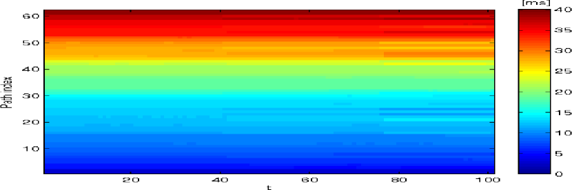
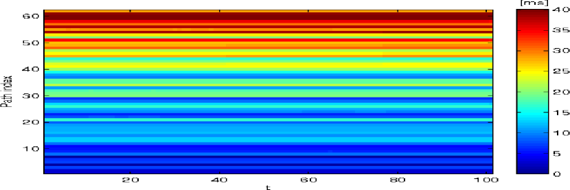
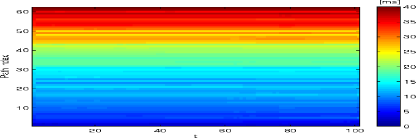
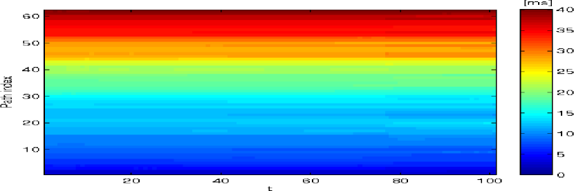
Figure 3: True and predicted delay map for $62$ paths in the Internet-2 dataset [1] over an interval of $100$ minutes. (Top-left) True delays; (Top-right) network kriging [17]; (Bottom-left) difussion wavelets [18]; and (Bottom-right) KKF [45]. Delays of several paths change slightly around $t=80$, but this change is only discernible from the delay predictions offered by KKF. Delay maps summarize the network state, and are useful tools aiding operational decision in network monitoring and control stations [45].

The spatio-temporal model set forth earlier can provide a better estimate of ${\bm{\chi}_{t}}$ by efficiently processing both present and past measurements jointly. Towards this end, a Kalman filter is employed in [45], which at time $t$ yields the following update equations

$$\hat{{\bm{\chi}}}_{t} :=\mathbb{E}^{*}\left[{\bm{\chi}_{t}}|\mathcal{H}_{t}\right]=\hat{{\bm{\chi}}}_{t-1}+{\bf K}_{t}({\bf d}^{s}_{t}-{\mathbf{S}_{t}}\hat{{\bm{\chi}}}_{t-1})$$

$${\bf M}_{t} :=\mathbb{E}\left[({\bm{\chi}_{t}}-\hat{{\bm{\chi}}}_{t})({\bm{\chi}_{t}}-\hat{{\bm{\chi}}}_{t})^{\prime}\right]=({\bf I}_{P}-{\bf K}_{t}{\mathbf{S}_{t}})({\bf M}_{t-1}+{\mathbf{C}_{\bm{\nu}}})$$

where ${\bf K}_{t}:=({\bf M}_{t-1}+{\mathbf{C}_{\bm{\nu}}}){\bf S}^{\prime}_{t}\left[{\mathbf{S}_{t}}({\mathbf{C}_{\bm{\nu}}}+{\mathbf{C}_{\bm{\eta}}}+{\bf M}_{t-1}){\bf S}^{\prime}_{t}+\sigma^{2}{\bf I}_{S}\right]^{-1}$ is the so-termed Kalman gain. The final predictor, referred also as the kriged Kalman filter (KKF), is given by

$$\hat{{\bf d}}^{\bar{s}}_{t}:=\bar{{\bf S}}_{t}\hat{{\bm{\chi}}}_{t}+\bar{{\bf S}}_{t}{\mathbf{C}_{\bm{\nu}}}{\bf S}^{\prime}_{t}\left({\mathbf{S}_{t}}{\mathbf{C}_{\bm{\nu}}}{\bf S}^{\prime}_{t}+\sigma^{2}{\bf I}_{S}\right)^{-1}[{\bf d}^{s}_{t}-{\mathbf{S}_{t}}\hat{{\bm{\chi}}}_{t}]$$

and the prediction error covariance matrix is

$${\bf M}^{\bar{s}}_{t}:=\mathbb{E}\left[\left({\bf d}^{\bar{s}}_{t}-\hat{{\bf d}}^{\bar{s}}_{t}\right)\left({\bf d}^{\bar{s}}_{t}-\hat{{\bf d}}^{\bar{s}}_{t}\right)^{\prime}\right]=\sigma^{2}{\bf I}_{S}+\bar{{\bf S}}_{t}\left[\left({\bf M}_{t-1}+{\mathbf{C}_{\bm{\nu}}}+{\mathbf{C}_{\bm{\eta}}}\right)^{-1}+\frac{1}{\sigma^{2}}{\bf S}^{\prime}_{t}{\mathbf{S}_{t}}\right]^{-1}\bar{{\bf S}}^{\prime}_{t}.$$

The KKF framework for dynamic network delay cartography has several attractive features. First, the KKF yields the LMMSE estimate even for non-Gaussian distributed noise. The Kalman filter step also allows for a $\tau$-step prediction given by $\hat{{\bf d}}_{t+\tau}=\hat{{\bm{\chi}}}_{t}$, which can be useful for preemptive routing and congestion control algorithms, as well as for extrapolating missing measurements. Second, the KKF framework provides a metric, namely the error covariance matrix ${\bf M}^{\bar{s}}_{t}$, for choosing the paths to be measured at each $t$, which define the selection matrix ${\mathbf{S}_{t}}$. In the present setting, it turns out that the D-optimal design metric $\log\det{\bf M}^{\bar{s}}_{t}$ is monotonic and supermodular with respect to the set $\mathcal{S}$ [45]. Thus, a simple greedy algorithm with complexity $\mathcal{O}(PS^{3})$ can be employed to find the set of paths that are at least 63% optimal [42]; see Fig. 4. Consequently, the technique can be readily applied to large-scale networks since the complexity increases only linearly with $P$. The framework also admits related problem formulations such as selecting the best set of monitors (nodes) capable of measuring delay on all its outgoing paths. This represents a significant departure from state-of-the-art delay prediction/tracking methods [17, 18], where path selection is heuristic. Note that training is required to estimate the model parameters ${\mathbf{C}_{\bm{\eta}}}$ and $\alpha$. To this end, empirical estimation techniques similar to those in [41] can be adapted to the present case.

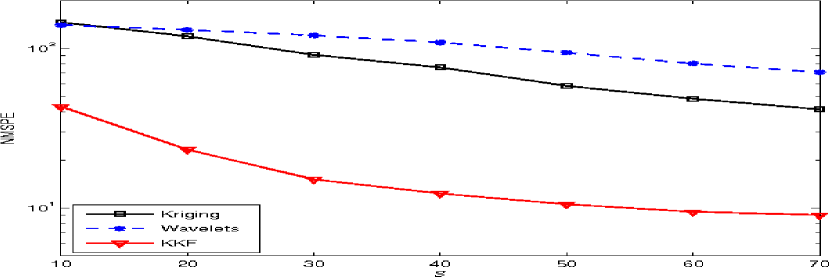
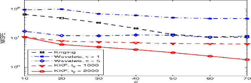
Figure 4: Delay cartography using the NZ-AMP dataset [2], which includes path delays collected over a month for an IP network where $P=186$ and $N=30$ [45]. Normalized mean-square prediction error (NMSPE) as a function of $S$. (Left) Random path selection; and (Right) “Optimal” path selection, that is, using heuristic or approximate algorithms specified for each algorithm. Observe further that the performance of the KKF improves as the length of the training interval $t_{T}$ increases.

III Dynamic Anomalography

This section switches gears to anomalography, the problem of unveiling and mapping-out network traffic anomalies across flows and time given link-level traffic measurements. This is a crucial monitoring task towards engineering network traffic, since anomalies can result in congestion and limit QoS provisioning.

III-A Traffic modeling

Consider a backbone IP network where $\cal{N}$ and $\mathcal{L}$ denote the sets of nodes (routers) and physical links of cardinality $|{\cal N}|=N$ and $|\mathcal{L}|=L$, respectively. The operational goal of the network is to transport a set of OD traffic flows $\cal{F}$ (with $|\mathcal{F}|=F$) associated with specific OD (ingress-egress router) pairs. Single-path routing is adopted here, meaning a given flow’s traffic is carried through multiple links connecting the corresponding source-destination pair along a single path. Accordingly, over a discrete time horizon $t\in[1,T]$ the measured link counts ${\bf X}:=[x_{l,t}]\in\mathbb{R}^{L\times T}$ and (unobservable) OD flow traffic matrix ${\bf Z}:=[z_{f,t}]\in\mathbb{R}^{F\times T}$, are thus related through ${\bf X}={\bf R}{\bf Z}$ [cf. (2)]. Unless otherwise stated, the routing matrix ${\bf R}$ is assumed given, since it can be otherwise estimated using traceroute or topology inference algorithms [24]. It is also fat, as for backbone networks the number of OD flows is much larger than the number of physical links $(F\gg L)$. A cardinal property of the traffic matrix is noteworthy. Common temporal patterns across OD traffic flows in addition to their almost periodic behavior, render most rows (respectively columns) of the traffic matrix linearly dependent, and thus ${\bf Z}$ typically has low rank. This intuitive property has been extensively validated with real network data; see Fig. 5 and e.g., [33].

Figure 5: Volumes of $6$ representative (out of $121$ total) OD flows, taken from the operation of Internet-2 during a seven-day period [1]. Temporal periodicities and correlations across flows are apparent. As expected, in this case ${\bf Z}$ can be well approximated by a low-rank matrix, since its normalized singular values decay rapidly to zero.

It is not uncommon for some of the OD flow rates to experience unexpected abrupt changes. These so-termed traffic volume anomalies are typically due to (unintentional) network equipment misconfiguration or outright failure, unforeseen behaviors following routing policy modifications, or, cyberattacks (e.g., DoS attacks) which aim at compromising the services offered by the network [55, 33]. Let $a_{f,t}$ denote the unknown amount of anomalous traffic in flow $f$ at time $t$. Explicitly accounting for the presence of anomalous flows, the measured traffic carried by link $l$ is then given by $y_{l,t}=\sum_{f\in\cal{F}}r_{l,f}(z_{f,t}+a_{f,t})+\epsilon_{l,t},~{}t=1,...,T$, where the noise variables $\epsilon_{l,t}$ capture measurement errors and unmodeled dynamics. Traffic volume anomalies are (unsigned) sudden changes in OD flow’s traffic, and as such their effect can span multiple links in the network. A key difficulty in unveiling anomalies from link-level measurements only is that oftentimes, clearly discernible anomalous spikes in the flow traffic can be masked through “destructive interference” of the superimposed OD flows [33]. An additional challenge stems from missing link-level measurements $y_{l,t}$, an unavoidable operational reality affecting most traffic engineering tasks that rely on (indirect) measurement of traffic matrices [56, 47]. To model missing link measurements, collect the tuples $(l,t)$ associated with the available observations $y_{l,t}$ in the set $\Omega\subseteq[1,2,...,L]\times[1,2,...,T]$. Introducing the matrices ${\bf Y}:=[y_{l,t}],{\bf E}:=[\epsilon_{l,t}]\in\mathbb{R}^{L\times T}$, and ${\bf A}:=[a_{f,t}]\in\mathbb{R}^{F\times T}$, the (possibly incomplete) set of link-traffic measurements can be expressed in compact matrix form as

$$\mathcal{P}_{\Omega}({\bf Y})=\mathcal{P}_{\Omega}({\bf X}+{\bf R}{\bf A}+{\bf E})$$ (9)

where the sampling operator $\mathcal{P}_{\Omega}(.)$ sets the entries of its matrix argument not in $\Omega$ to zero, and keeps the rest unchanged. Since the objective here is not to estimate the OD flow traffic matrix ${\bf Z}$, (9) is expressed in terms of the nominal (anomaly-free) link-level traffic rates ${\bf X}$, which inherits the low-rank property of ${\bf Z}$. Anomalies in ${\bf A}$ are expected to occur sporadically over time, and last for a short time relative to the (possibly long) measurement interval $[1,T]$. In addition, only a small fraction of the flows is supposed to be anomalous at a any given time instant. This renders the anomaly traffic matrix ${\bf A}$ sparse across both rows (flows) and columns (time).

III-B Unveiling anomalies via sparsity and low rank

Given link-level traffic measurements $\mathcal{P}_{\Omega}({\bf Y})$ adhering to (9), dynamic anomalography is a critical network monitoring task that aims at accurately estimating the anomaly matrix ${\bf A}$. As argued next, capitalizing on the sparsity of ${\bf A}$ and the low-rank property of ${\bf X}$ will be instrumental in achieving this ambitious goal. From a network cartography vantage point, the resultant estimated map $\hat{{\bf A}}$ offers a depiction of the network’s “health state” along both the flow and time dimensions. If $|\hat{a}_{f,t}|>0$, the $f$-th flow at time $t$ is deemed anomalous, otherwise it is healthy. This joint estimation-detection task not only allows one to identify the time of the anomaly in addition to the affected flows, but also to estimate its magnitude which hints to the importance of the anomaly event. By examining ${\bf R}$ the network operator can immediately determine the links carrying the anomalous flows. Subsequently, planned contingency measures involving traffic-engineering algorithms can be implemented to address network congestion.

The low-rank property of the traffic matrix ${\bf Z}$ (and ${\bf X}$) is at the heart of the seminal network anomaly detection approach in [33]. In the absence of missing data, the method therein adopts principal component analysis (PCA) to decompose the link traffic ${\bf Y}=[{\bf y}_{1},\ldots,{\bf y}_{T}]$ into nominal and anomalous components (also known as modeled and residual traffic). For instance, if most of the variance in ${\bf Y}$ is captured by $r\ll\min(L,T)$ dominant principal components, then by construction the nominal subspace $\mathcal{S}_{n}$ is spanned by the $r$ dominant right singular vectors of ${\bf Y}^{\prime}$ (cf. the low rank assumption). Naturally, the anomalous subspace $\mathcal{S}_{a}$ corresponds to the orthogonal complement, i.e., $\mathcal{S}_{a}:=\mathcal{S}_{n}^{\perp}$. In the operational phase, an anomaly is declared at time $t$ when $\|\mathbf{P}_{\mathcal{S}_{a}}{\bf y}_{t}\|_{2}^{2}$ exceeds a given threshold, where $\mathbf{P}_{\mathcal{S}_{a}}$ is an orthogonal projection matrix onto $\mathcal{S}_{a}$. Subsequently, a single anomalous flow is identified after running a greedy algorithm, and an estimate of the amount of anomalous traffic is obtained as a byproduct. Likewise, the spatial approach within the network anomography framework [55] forms the matrix $\mathbf{P}_{\mathcal{S}_{a}}{\bf Y}$ of link anomalies, thus exploiting the correlation between traffic across different links. Temporal approaches obtain link anomalies as ${\bf Y}{\bf T}$ instead, where ${\bf T}$ is a linear operator which judiciously filters the traffic time series per link (implementing an “anomaly-pass” filter). Several choices for ${\bf T}$ are proposed to this end, based on different forms of temporal analysis including autoregressive integrated moving average (ARIMA), wavelets, and fast Fourier transform (FFT). Different from [33], the inference algorithm in [55] capitalizes on the sparsity of ${\bf A}$ to estimate the anomaly map by e.g., solving in the spatial case

$$\hat{{\bf A}}:=\arg\min_{{\bf A}}\|{\bf A}\|_{1},\quad\textrm{s. t. }\>\mathbf{P}_{\mathcal{S}_{a}}{\bf Y}={\bf R}{\bf A}.$$

Network anomography algorithms can be extended to accommodate routing changes across time; see [55] for further details and comprehensive performance tests.

Recently, a natural estimator leveraging the low rank property of ${\bf X}$ and the sparsity of ${\bf A}$ was put forth in [38], which can be found at the crossroads of CS [23] and timely low-rank plus sparse matrix decompositions [10, 14]. The idea is to fit the incomplete data $\mathcal{P}_{\Omega}({\bf Y})$ to the model ${\bf X}+{\bf R}{\bf A}$ [cf. (9)] in the LS error sense, as well as minimize the rank of ${\bf X}$, and the number of nonzero entries of ${\bf A}$ measured by its $\ell_{0}$-(pseudo) norm. Unfortunately, albeit natural both rank and $\ell_{0}$-norm criteria are in general NP-hard to optimize. Typically, the nuclear norm $\|{\bf X}\|_{*}:=\sum_{k}\sigma_{k}({\bf X})$ ($\sigma_{k}({\bf X})$ denotes the $k$-th singular value of ${\bf X}$) and the $\ell_{1}$-norm $\|{\bf A}\|_{1}$ are adopted as surrogates [25, 11], since they are the closest convex approximants to $\textrm{rank}({\bf X})$ and $\|{\bf A}\|_{0}$, respectively. Accordingly, one solves

$$\min_{\{{\bf X},{\bf A}\}}\|\mathcal{P}_{\Omega}({\bf Y}-{\bf X}-{\bf R}{\bf A})\|_{F}^{2}+\lambda_{\ast}\|{\bf X}\|_{*}+\lambda_{1}\|{\bf A}\|_{1}$$ (10)

where $\lambda_{*},\lambda_{1}\geq 0$ are rank- and sparsity-controlling parameters. While a non-smooth optimization problem, being convex (10) is appealing. An efficient accelerated proximal gradient algorithm with quantifiable iteration complexity was developed to unveil network anomalies [39]. Interestingly, (10) also offers a cleansed estimate of the link-level traffic $\hat{{\bf X}}$, that could be subsequently utilized for network tomography tasks. In addition, (10) jointly exploits the spatio-temporal correlations in the link traffic as well as the sparsity of the anomalies, through an optimal single-shot estimation-detection procedure that has been shown to outperform the algorithms in [33] and [55] (that decouple the estimation and detection steps).

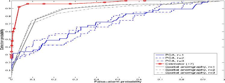
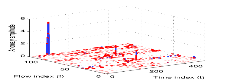
Figure 6: Unveiling anomalies from Internet-2 data [1]. (Left) ROC curve comparison between (10) and the PCA methods in [33, 55], for different values of $r:=\textrm{dim}(\mathcal{S}_{n})$. Leveraging sparsity and low rank jointly leads to improved performance. (Right) In red, the estimated anomaly map $\hat{{\bf A}}$ obtained via (10) superimposed to the “true” anomalies shown in blue [37].

Before moving on to distributed implementations, it is instructive to elaborate on the generality of (10). When there is no missing data and ${\bf X}=\mathbf{0}_{L\times T}$, one is left with an under-determined sparse signal recovery problem typically encountered with CS; see e.g., [23]. The decomposition ${\bf Y}={\bf X}+{\bf A}$ corresponds to principal component pursuit (PCP), also referred to as robust PCA [10, 14]. For the idealized noise-free setting (${\bf E}=\mathbf{0}_{L\times T}$), sufficient conditions for exact recovery of the unknowns are available for both of the aforementioned special cases [11, 10, 14]. However, the superposition of a low-rank plus a compressed sparse matrix in (9) further challenges identifiability of $\{{\bf X},{\bf A}\}$; see [39] for early results. Going back to the CS paradigm, even when ${\bf X}$ is nonzero one could envision a variant where the measurements are corrupted with correlated (low-rank) noise [15]. Last but not least, when ${\bf A}=\mathbf{0}_{F\times T}$ and ${\bf Y}$ is noisy, the recovery of ${\bf X}$ subject to a rank constraint is nothing but PCA – arguably, the workhorse of high-dimensional data analytics. This same formulation is adopted for low-rank matrix completion, to impute the missing entries of a low-rank matrix observed in noise, i.e., $\mathcal{P}_{\Omega}({\bf Y})=\mathcal{P}_{\Omega}({\bf X}+{\bf E})$ [12].

III-C In-network distributed processing

Implementing (10) presumes that network nodes continuously communicate their link traffic measurements to a central monitoring station, which uses their aggregation in $\mathcal{P}_{\Omega}({\bf Y})$ to unveil anomalies. While for the most part this is the prevailing operational paradigm adopted in current networks, it is fair to say there are limitations associated with this architecture. For instance, fusing all this information may entail excessive protocol overheads. Moreover, minimizing the exchanges of raw measurements may be desirable to reduce unavoidable communication errors that translate to missing data. Solving (10) centrally raises robustness concerns as well, since the central monitoring station represents an isolated point of failure.

These reasons motivate well devising fully-distributed iterative algorithms for dynamic anomalography, embedding the network anomaly detection functionality to the routers. In a nutshell, per iteration nodes $n\in\mathcal{N}$ carry out simple computational tasks locally, relying on their own link count measurements (a submatrix ${\bf Y}_{n}$ within ${\bf Y}=[{\bf Y}_{1}^{\prime},\ldots,{\bf Y}_{N}^{\prime}]^{\prime}$ corresponding to router $n$’s links). Subsequently, local estimates are refined after exchanging messages only with directly connected neighbors, which facilitates percolation of local information to the whole network. The end goal is for network nodes to consent on a global map of network anomalies $\hat{{\bf A}}$, and attain (or at least come close to) the estimation performance of the centralized counterpart (10) which has all data $\mathcal{P}_{\Omega}({\bf Y})$ available.

Problem (10) is not amenable for distributed implementation due to the non-separable nuclear norm present in the cost function. If an upper bound $\textrm{rank}(\hat{\bf X})\leq\rho$ is a priori available [recall $\hat{\bf X}$ is the estimated link-level traffic obtained via (10)], (10)’s search space is effectively reduced and one can factorize the decision variable as ${\bf X}={\bf P}{\bf Q}^{\prime}$, where ${\bf P}$ and ${\bf Q}$ are $L\times\rho$ and $T\times\rho$ matrices, respectively. Again, it is possible to interpret the columns of ${\bf X}$ (viewed as points in $\mathbb{R}^{L}$) as belonging to a low-rank nominal subspace $\mathcal{S}_{n}$, spanned by the columns of ${\bf P}$. The rows of ${\bf Q}$ are thus the projections of the columns of ${\bf X}$ onto $\mathcal{S}_{n}$. Next, consider the following alternative characterization of the nuclear norm (see e.g. [46])

$$\|{\bf X}\|_{*}:=\min_{\{{\bf P},{\bf Q}\}}~{}~{}~{}\frac{1}{2}\left(\|{\bf P}\|_{F}^{2}+\|{\bf Q}\|_{F}^{2}\right),\quad\text{s. t.}~{}~{}~{}{\bf X}={\bf P}{\bf Q}^{\prime}$$ (11)

where the optimization is over all possible bilinear factorizations of ${\bf X}$, so that the number of columns $\rho$ of ${\bf P}$ and $\mathbf{Q}$ is also a variable. Leveraging (11), the following reformulation of (10) provides an important first step towards obtaining a distributed anomalography algorithm

$$\min_{\{{\bf P},{\bf Q},{\bf A}\}}\sum_{n=1}^{N}\left[\|\mathcal{P}_{\Omega_{n}}({\bf Y}_{n}-{\bf P}_{n}{\bf Q}^{\prime}-{\bf R}_{n}{\bf A})\|_{F}^{2}+\frac{\lambda_{*}}{2N}\left(N\|{\bf P}_{n}\|_{F}^{2}+\|{\bf Q}\|_{F}^{2}\right)+\frac{\lambda_{1}}{N}\|{\bf A}\|_{1}\right]$$ (12)

which is non-convex due to the bilinear terms ${\bf P}_{n}{\bf Q}^{\prime}$, and where ${\bf R}:=\left[{\bf R}_{1}^{\prime},\ldots,{\bf R}_{N}^{\prime}\right]^{\prime}$ is partitioned into local routing tables available per router $n$. Adopting the separable Frobenius-norm regularization in (12) comes with no loss of optimality relative to (10), provided $\textrm{rank}(\hat{\bf X})\leq\rho$. By finding the global minimum of (12) [which could have considerably less variables than (10)], one can recover the optimal solution of (10). But since (12) is non-convex, it may have stationary points which need not be globally optimum. As asserted in [38, Prop. 1] however, if a stationary point $\{\bar{{\bf P}},\bar{{\bf Q}},\bar{{\bf A}}\}$ of (12) satisfies $\|\mathcal{P}_{\Omega}({\bf Y}-\bar{{\bf P}}\bar{{\bf Q}}^{\prime}-\bar{{\bf A}})\|<\lambda_{*}$, then $\{\hat{\bf X}:=\bar{{\bf P}}\bar{{\bf Q}}^{\prime},\hat{{\bf A}}:=\bar{{\bf A}}\}$ is the globally optimal solution of (10). Note that for sufficiently small $\rho$ the residual $\|\mathcal{P}_{\Omega}({\bf Y}-\bar{{\bf P}}\bar{{\bf Q}}^{\prime}-\bar{{\bf A}})\|$ becomes large, and the qualification inequality is violated [unless $\lambda_{*}$ is large enough, in which case a sufficiently low-rank solution to (10) is expected]. The condition on the residual implicitly enforces $\textrm{rank}(\hat{\bf X})\leq\rho$, which is necessary for the equivalence between (10) and (12).

To decompose the cost in (12), in which summands inside the square brackets are coupled through the global variables $\{{\bf Q},{\bf A}\}$, introduce auxiliary copies $\{{\bf Q}_{n},{\bf A}_{n}\}_{n=1}^{N}$ representing local estimates of $\{{\bf Q},{\bf A}\}$, one per node $n$. These local copies along with consensus constraints yield the distributed estimator

$$\min_{\{{\bf P}_{n},{\bf Q}_{n},{\bf A}_{n}\}} \sum_{n=1}^{N}\left[\|\mathcal{P}_{\Omega_{n}}({\bf Y}_{n}-{\bf P}_{n}{\bf Q}_{n}^{\prime}-{\bf R}_{n}{\bf A}_{n})\|_{F}^{2}+\frac{\lambda_{*}}{2N}\left(N\|{\bf P}_{n}\|_{F}^{2}+\|{\bf Q}_{n}\|_{F}^{2}\right)+\frac{\lambda_{1}}{N}\|{\bf A}_{n}\|_{1}\right]$$ (13)

s. t. $$\quad{\bf Q}_{n}={\bf Q}_{m},\>{\bf A}_{n}={\bf A}_{m}\quad m\textrm{ linked with }n\in\mathcal{N}$$

which is equivalent to (12) provided the network topology graph is connected. Even though consensus is a fortiori imposed within neighborhoods, it extends to the whole (connected) network and local estimates agree on the global solution of (12). Exploiting the separable structure of (13), a general framework for in-network sparsity-regularized rank minimization was put forth in [38]. Specifically, distributed iterations were obtained after adopting the alternating-direction method of multipliers (ADMM), an iterative Lagrangian method well-suited for parallel processing [9]. In a nutshell, local tasks per iteration $k=1,2,\ldots$ entail solving small unconstrained quadratic programs to refine the normal subspace ${\bf P}_{n}[k]$, in addition to soft-thresholding operations to update the anomaly maps ${\bf A}_{n}[k]$ per router. Each iteration, routers exchange their estimates $\{{\bf Q}_{n}[k],{\bf A}_{n}[k]\}$ only with directly connected neighbors. This way the communication overhead remains affordable, and independent of the network size $N$.

When employed to solve non-convex problems such as (13), so far ADMM offers no convergence guarantees. However, there is ample experimental evidence in the literature that supports empirical convergence of ADMM, especially when the non-convex problem at hand exhibits “favorable” structure. For instance, (13) is a linearly constrained bi-convex problem with potentially good convergence properties – extensive numerical tests in [38] demonstrate that this is indeed the case. While establishing convergence remains an open problem, one can still prove that upon convergence the distributed iterations attain consensus and global optimality, offering the desirable centralized performance guarantees [38].

III-D Real-time anomaly trackers

Monitoring of large-scale IP networks necessitates massive recollection of data which far outweigh the ability of modern computers to store and analyze them in real time. In addition, nonstationarities due to routing changes and missing data further challenge identification of anomalies. In dynamic networks routing tables are constantly readjusted to effect traffic load balancing and avoid congestion caused by e.g., traffic anomalies. To account for slowly time-varing routing tables, let ${\bf R}_{t}\in\mathbb{R}^{L\times F}$ denote the routing matrix at time $t$. In this dynamic setting, the partially observed link counts at time $t$ adhere to $\mathcal{P}_{\Omega_{t}}({\bf y}_{t})=\mathcal{P}_{\Omega_{t}}({\bf x}_{t}+{\bf R}_{t}{\bf a}_{t}+\bm{\epsilon}_{t}),~{}t=1,2,\ldots$, where the link-level traffic ${\bf x}_{t}:={\bf R}_{t}{\bf z}_{t}$. In general, routing changes may alter a link load considerably by e.g., routing traffic completely away from a specific link. Therefore, even though the OD flow vectors $\{{\bf z}_{t}\}$ live in a low-dimensional subspace, the same may not be true for the $\{{\bf x}_{t}\}$ when the routing updates are major and frequent. In backbone networks however, routing changes are sporadic relative to the time-scale of data acquisition used for network monitoring tasks. For example, data collected from the operation of Internet-2 network reveals that only a few rows of ${\bf R}_{t}$ change per week [1]. It is thus safe to assume that $\{{\bf x}_{t}\}$ still lies in a low-dimensional subspace, and exploit the spatio-temporal correlations of the observations to identify the anomalies in real-time.

On top of the previous arguments, in practice link measurements are acquired sequentially in time, which motivates updating previously obtained estimates rather than re-computing new ones from scratch each time a new datum becomes available. The goal is then to recursively estimate $\{\hat{{\bf x}}_{t},\hat{{\bf a}}_{t}\}$ at time $t$ from historical observations $\{\mathcal{P}_{\Omega_{\tau}}({\bf y}_{\tau})\}_{\tau=1}^{t}$, naturally placing more importance on recent measurements. To this end, one possible adaptive counterpart to (12) is the exponentially-weighted LS estimator found by minimizing the empirical cost [37]

$$\min_{\{{\bf P},{\bf Q},{\bf A}\}}\sum_{\tau=1}^{t}\beta^{t-\tau}\left[\|\mathcal{P}_{\Omega_{\tau}}({\bf y}_{\tau}-{\bf P}{\bf q}_{\tau}-{\bf R}_{\tau}{\bf a}_{\tau})\|_{2}^{2}+\frac{\lambda_{\ast}}{2\sum_{u=1}^{t}\beta^{t-u}}\|{\bf P}\|_{F}^{2}+\frac{\lambda_{\ast}}{2}\|{\bf q}_{\tau}\|_{2}^{2}+\lambda_{1}\|{\bf a}_{\tau}\|_{1}\right]$$ (14)

in which $0<\beta\leq 1$ is the so-termed forgetting factor. When $\beta<1$ data in the distant past are exponentially downweighted, which facilitates tracking network anomalies in nonstationary environments. For static routing (${\bf R}_{t}={\bf R}$) and infinite memory $(\beta=1)$, the formulation (14) coincides with the batch estimator (12). A provably convergent online algorithm for dynamic anomalography is developed in [37], based on alternating minimization of (14); see Fig. 7. Each time a new datum is acquired, anomaly estimates are formed via the Lasso [51], and the low-rank nominal traffic subspace is refined using recursive LS. For situations were reducing computational complexity is critical, an online stochastic gradient algorithm based on Nesterov’s acceleration technique is developed as well [37].

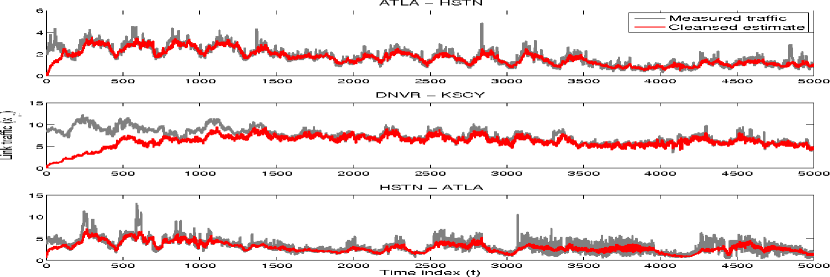
Figure 7: Unveiling anomalies in real time from Internet-2 data [1]. (Left) Measured link traffic and cleansed estimates for three representative links; and (Right) three rows of the estimated anomaly map $\hat{{\bf A}}$ corresponding to three anomalous flows [37].

Algorithms in [37] are closely related to timely robust subspace trackers, which aim at estimating a low-rank subspace ${\bf P}$ from grossly corrupted and possibly incomplete data, namely $\mathcal{P}_{\Omega_{t}}({\bf y}_{t})=\mathcal{P}_{\Omega_{t}}({\bf P}{\bf q}_{t}+{\bf a}_{t}+\bm{\epsilon}_{t}),~{}t=1,2,\ldots$. In the absence of sparse “outliers” $\{{\bf a}_{t}\}_{t=1}^{\infty}$, an online algorithm based on incremental gradient descent on the Grassmannian manifold of subspaces was put forth in [4]. The second-order RLS-type algorithm in [16] extends the seminal projection approximation subspace tracking (PAST) algorithm to handle missing data. When outliers are present, robust counterparts can be found in [15, 28]. Relative to all aforementioned works, the estimation problem (14) is more challenging due to the presence of the (compression) routing matrix ${\bf R}_{t}$; see [39] for fundamental identifiability issues related to the model (9).

IV Broadening the network atlas

Additional cartography instances are outlined in this section, including anomalography from flow measurements and network distance prediction. To exemplify the development of sensing infrastructure for situational awareness at the physical layer of wireless CR networks, the notion of RF cartography is introduced as well. All these problems can be tackled through SP methods subsumed by (10), namely PCP [14], low-rank matrix completion [12], the Lasso [51], and non-parametric versions of basis pursuit [7].

IV-A Unveiling anomalies from flow data

Since some networks nowadays collect OD flow (not link-level) measurements $z_{f,t}+a_{f,t}$ for at least part of their network (using e.g., the Netflow protocol), anomalies can be detected using temporal decomposition and standard change-detection approaches per flow. Leveraging the low-rank property of the traffic matrix and the sparsity of anomalies, anomalography from OD flow measurements was formulated as the PCP matrix decomposition problem and solved centrally in [3]; see also [38] for a distributed implementation of the PCP estimator aimed at scalable monitoring of networks.

IV-B Network distance prediction

End-to-end network distance information is critical towards enhancing QoS in Internet applications such as content distribution and peer-to-peer file sharing systems. Clients naturally prefer to establish connections with “closer” network resources or servers that are likely to respond faster. There are different metrics to quantify the distance between a pair of network nodes. The most common choices are defined in terms of latency (one-way delay and the so-termed round-trip time) or router hop-counts. Unfortunately, either probing or passively measuring all pairwise distances becomes infeasible in large-scale networks. Given those few affordable distance measurements, the problem of network distance prediction is to impute (that is interpolate) the missing entries in a highly-incomplete matrix of end-to-end distances.

If one collects the end-to-end latencies $d_{i,j}$ of source-sink pairs $(i,j)$ in a delay matrix ${\bf D}:=[d_{i,j}]\in\mathbb{R}^{N\times N}$, strong dependencies among path delays render ${\bf D}$ low rank; see e.g., [35] for an experimental validation with multiple datasets. Intuitively, correlations among rows and columns of ${\bf D}$ emerge because nearby nodes (e.g., those belonging to a common subnetwork) are connected to every other node through paths with significant overlap, possibly sharing common bottleneck links. The low-rank property of ${\bf D}$ along with the distributed-processing requirements of large-scale networks, motivated decentralized matrix-factorization [35] and nuclear-norm minimization [38] algorithms for network distance prediction. Different from schemes based on Euclidean embedding via multi-dimensional scaling [22], low-rank modeling does not require distances in ${\bf D}$ to be symmetric and satisfy the triangle inequality – properties that are oftentimes violated by network-related distances [34].

To avoid the excessive overhead of active probing mechanisms, one can leverage network monitors that passively observe router hop-counts from traffic traversing those monitored links; see e.g., [24] and references therein. Collect these hop-count measurements in the matrix ${\bf H}:=[h_{m,n}]\in\mathbb{N}^{M\times N}$, where $M$ is the number of monitors, and $N$ ($\gg M$) the total hosts observed. Because monitor $m$ only observes a fraction of the total network traffic, ${\bf H}$ will be depleted with missing entries. Despite typically having $\textrm{rank}({\bf H})=M$, ${\bf H}$ consists of low-rank column blocks, each corresponding to a subnetwork with access to the Internet core through a single border router. Recognizing this structure, a high-rank matrix completion algorithm that performs subspace clustering of incomplete hop-count data was put forth in [24], and shown to attain good performance both in theory and practice.

Different from the dynamic network delay cartography problem considered in Sec. II-B, network distance prediction approaches do not account for the temporal variations in the delays, and typically rely on batch imputation of the distance matrix of interest. The techniques used in Sec. II-B do not apply in this context either, since some path delays are never observed, and thus it is impossible to estimate the spatial covariance matrices (such as ${\mathbf{C}_{\bm{\eta}}}$ and ${\mathbf{C}_{\bm{\nu}}}$) completely.

IV-C RF cartography

In the domain of spectrum sensing for CR networks, RF cartography amounts to constructing in a distributed fashion: m1) global power spectral density (PSD) maps capturing the distribution of radiated power across space, time, and frequency; and m2) local channel gain (CG) maps offering the propagation medium per frequency from each node to any point in space. These maps enable identification of opportunistically available spectrum bands for re-use and handoff operation; as well as localization, transmit-power estimation, and tracking of primary user activities. While the focus here is on the construction of PSD maps, the interested reader is referred to [29] for a tutorial treatment on CG cartography.

A cooperative approach to RF cartography was introduced in [6], that builds on a basis expansion model of the PSD map $\Phi({\mathbf{x}},f)$ across space ${\mathbf{x}}\in\mathbb{R}^{2}$, and frequency $f$. Spatially-distributed CRs collect smoothed periodogram samples of the received signal at given sampling frequencies, based on which they want to determine the unknown expansion coefficients. Introducing a virtual spatial grid of candidate source locations, the estimation task can be cast as a linear LS problem with an augmented vector of unknown parameters. Still, the problem complexity (or effective degrees of freedom) can be controlled by capitalizing on two forms of sparsity: the first one introduced by the narrow-band nature of transmit-PSDs relative to the broad swaths of usable spectrum; and the second one emerging from sparsely located active radios in the operational space (due to the grid artifact). Nonzero entries in the parameter vector sought correspond to spatial location-frequency band pairs corresponding to active transmissions. All in all, estimating the PSD map and locating the active transmitters as a byproduct boils down to a variable selection problem. This motivates well employment of the Lasso for distributed sparse linear regression [38], an estimator also subsumed by (10) when ${\bf X}=\mathbf{0}_{L\times T}$, $T=1$, and the regression matrix ${\bf R}$ has a specific structure that depends on the chosen bases and path-loss propagation model.

Sparse total LS variants are also available to cope with uncertainty in the regression matrix, arising due to inaccurate channel estimation and grid-mismatch effects [29]. Nonparametric spline-based PSD map estimators [7] have been also shown effective in capturing general propagation characteristics including both shadowing and fading; see also Fig. 8 for an actual PSD atlas spanning $14$ frequency sub-bands.

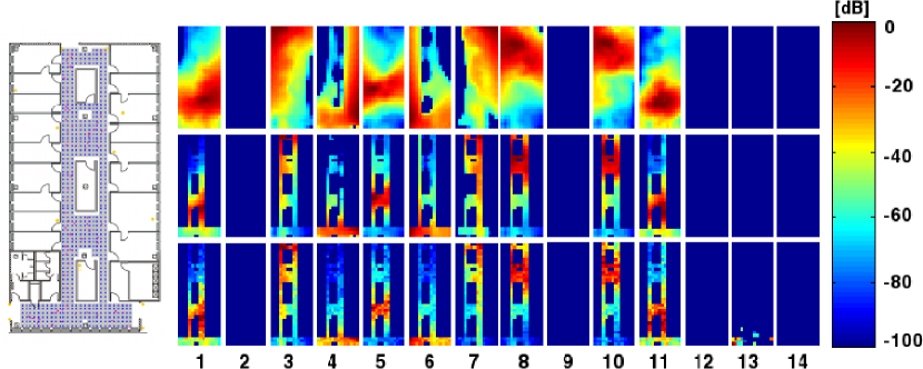
Figure 8: Spline-based RF cartography using the dataset [31]. (Left) Detailed floor plan schematic including the location of $N=166$ sensing radios; (Right-bottom) original measurements spanning $14$ frequency sub-bands; (Right-center) estimated maps over the surveyed area; and (Right-top) extrapolated maps. The proposed estimator is capable of recovering the $9$ (out of $14$ total) center frequencies that are being utilized for transmission. It accurately recovers the power levels in the surveyed area with a smooth extrapolation to zones were there are no measurements, and suggests possible locations for the transmitters [7].

V Concluding remarks

In this tutorial, the concept of dynamic network cartography is introduced as a framework to construct maps of the dynamically evolving network state, in an efficient and scalable manner even for large-scale heterogeneous networks. Focus is placed on key tasks geared to obtaining full yet succinct representation of network state metrics such as link traffic and path delays, as well as prompt and accurate identification of network anomalies from possibly partial and corrupted measurement data.

Looking forward, the unceasing demand for continuous situational awareness calls for innovative and large-scale distributed SP algorithms, complemented by collaborative and adaptive monitoring platforms to accomplish the objectives of network management and control. Avenues where significant impact can be made include: i) judicious design of critical cognition infrastructure to sense, learn, and adapt to the environment where networks operate; ii) development of scalable tools for distilling, summarizing, and tracking the network state for the purpose of network management; iii) ensuring robustness in the face of missing and grossly-corrupted network data, in addition to possibly malicious attacks; and iv) developing effective network adaptation techniques based on global network inference, further impacting protocol designs, network taxonomy, and categorization.

References

- [1] [Online]. Available: http://www.internet2.edu
- [2] [Online]. Available: http://erg.cs.waikato.ac.nz/amp/matrix.php/ipv4/latency/NZ
- [3] A. Abdelkefi, Y. Jiang, W. Wang, A. Aslebo, and O. Kvittem, “Robust traffic anomaly detection with principal component pursuit,” in Proc. of the ACM CoNEXT Student Workshop, Philadelphia, PA, Nov. 2010.
- [4] L. Balzano, R. Nowak, and B. Recht, “Online identification and tracking of subspaces from highly incomplete information,” in Proc. of Allerton Conf. on Communication, Control, and Computing, Monticello, IL, 2010.
- [5] V. W. Bandara and A. P. Jayasumana, “Extracting baseline patterns in internet traffic using robust principal components,” in Proc. IEEE Intl. Conf. on Local Computer Netw., Bonn, Germany, 2011.
- [6] J. A. Bazerque and G. B. Giannakis, “Distributed spectrum sensing for cognitive radio networks by exploiting sparsity,” IEEE Trans. Signal Process., vol. 58, pp. 1847–1862, Mar. 2010.
- [7] J. A. Bazerque, G. Mateos, and G. B. Giannakis, “Group Lasso on splines for spectrum cartography,” IEEE Trans. Signal Process., vol. 59, pp. 4648–4663, Oct. 2011.
- [8] M. Belkin, P. Niyogi, and V. Sindhwani, “Manifold regularization: A geometric framework for learning from labeled and unlabeled examples,” J. Mach. Learn. Res., vol. 7, pp. 2399–2434, Dec. 2006.
- [9] D. P. Bertsekas and J. N. Tsitsiklis, Parallel and Distributed Computation: Numerical Methods. Athena-Scientific, 1999.
- [10] E. J. Candes, X. Li, Y. Ma, and J. Wright, “Robust principal component analysis?” Journal of the ACM, vol. 58, no. 1, pp. 1–37, 2011.
- [11] E. J. Candes and T. Tao, “Decoding by linear programming,” IEEE Trans. Info. Theory, vol. 51, no. 12, pp. 4203–4215, 2005.
- [12] E. Candes and Y. Plan, “Matrix completion with noise,” Proc. of the IEEE, vol. 98, pp. 925–936, 2009.
- [13] R. Castro, M. Coates, G. Liang, R. Nowak, and B. Yu, “Network tomography: Recent developments,” Statist. Sci., vol. 19, no. 3, pp. 499–517, 2004.
- [14] V. Chandrasekaran, S. Sanghavi, P. R. Parrilo, and A. S. Willsky, “Rank-sparsity incoherence for matrix decomposition,” SIAM J. Optim., vol. 21, no. 2, pp. 572–596, 2011.
- [15] Q. Chenlu and N. Vaswani, “Recursive sparse recovery in large but correlated noise,” in Proc. of Allerton Conf. on Communication, Control, and Computing, Monticello, IL, 2011.
- [16] Y. Chi, Y. C. Eldar, and R. Calderbank, “Petrels: Subspace estimation and tracking from partial observations,” in Proc. of IEEE International Conference on Acoustics, Speech and Signal Processing, Kyoto, Japan, Mar. 2012.
- [17] D. Chua, E. Kolaczyk, and M. Crovella, “Network kriging,” IEEE J. Sel. Areas Commun., vol. 24, 2006.
- [18] M. Coates, Y. Pointurier, and M. Rabbat, “Compressed network monitoring for IP and all-optical networks,” in Proc. ACM Internet Measurement Conf., San Diego, CA, Oct. 2007.
- [19] G. Conti, Security Data Visualization: Graphical Techniques for Network Analysis. No Starch Press, 2007.
- [20] J. Cortés, “Distributed Kriged Kalman filter for spatial estimation,” vol. 54, no. 12, pp. 2816–2827, Dec. 2009.
- [21] N. Cressie, “The origins of kriging,” Mathematical Geology, vol. 22, no. 3, pp. 239–252, 1990.
- [22] F. Dabek, R. Cox, F. Kaashoek, and R. Morris, “Vivaldi: A decentralized network coordinate system,” in Proc. of ACM SIGCOMM, Portland, OR, Aug. 2004.
- [23] D. L. Donoho, “Compressed sensing,” IEEE Trans. Info. Theory, vol. 52, no. 4, pp. 1289 –1306, Apr. 2006.
- [24] B. Eriksson, L. Balzano, and R. Nowak, “High-rank matrix completion,” in Proc. of Intl. Conf. on Artificial Intell. and Stat., La Palma, Canary Islands, Apr. 2012.
- [25] M. Fazel, “Matrix rank minimization with applications,” Ph.D. dissertation, Electrical Eng. Dept., Stanford University, 2002.
- [26] P. A. Forero, K. Rajawat, and G. B. Giannakis, “Semi-supervised dictionary learning for network-wide link load prediction,” in Proc. Cognitive Information Processing Workshop, Baiona, Spain, May 2012.
- [27] J. Friedman, T. Hastie, H. Höfling, and R. Tibshirani, “Pathwise coordinate optimization,” The Annals of Applied Statistics, vol. 1, no. 2, pp. 302–332, 2007.
- [28] J. He, L. Balzano, and A. Szlam, “Incremental gradient on the Grassmannian for online foreground and background separation in subsampled video,” in Proc. of IEEE Conference on Computer Vision and Pattern Recognition, Providence, Rhode Island, Jun. 2012.
- [29] S.-J. Kim, E. Dall’Anese, J. A. Bazerque, K. Rajawat, and G. B. Giannakis, “Advances in spectrum sensing and cross-layer design for cognitive radio networks,” Elsevier, E-Reference Signal Processing, 2012.
- [30] S.-J. Kim, E. Dall’Anese, and G. B. Giannakis, “Cooperative spectrum sensing for cognitive radios using Kriged Kalman filtering,” IEEE Jrnl. Sel. Topics in Signal Process., vol. 5, no. 1, pp. 24–36, Feb. 2011.
- [31] T. King, S. Kopf, T. Haenselmann, C. Lubberger, and W. Effelsberg, “CRAWDAD data set mannheim/compass (v. 2008-04-11),” Downloaded from http://crawdad.cs.dartmouth.edu/mannheim/compass, Apr. 2008.
- [32] E. D. Kolaczyk, Statistical Analysis of Network Data: Methods and Models. Springer, 2009.
- [33] A. Lakhina, M. Crovella, and C. Diot, “Diagnosing network-wide traffic anomalies,” in Proc. of ACM SIGCOMM, Portland, OR, Aug. 2004.
- [34] S. Lee, Z. Zhang, S. Sahu, and D. Saha, “On suitability of Euclidean embedding Internet hosts,” in SIGMETRICS, Saint Malo, France, Jun. 2006.
- [35] Y. Liao, P. Geurts, and G. Leduc, “Network distance prediction based on decentralized matrix factorization,” in Proc. of IFIP Networking Conf., Chennai, India, May 2010.
- [36] J. Mairal, J. Bach, J. Ponce, and G. Sapiro, “Online learning for matrix factorization and sparse coding,” Jrnl. of Machine Learning Research, vol. 11, pp. 19–60, Jan. 2010.
- [37] M. Mardani, G. Mateos, and G. B. Giannakis, “Dynamic anomalography: Tracking network anomalies via sparsity and low rank,” IEEE Jrnl. Sel. Topics in Signal Process., 2012, see also arXiv:1208.4043v1 [cs.NI].
- [38] ——, “In-network sparsity-regularized rank minimization: Applications and algorithms,” IEEE Trans. Signal Process., 2012, see also arXiv:1203.1507v1 [cs.MA].
- [39] ——, “Recovery of low-rank plus compressed sparse matrices with application to unveiling traffic anomalies,” IEEE Trans. Info. Theory, 2012, see also arXiv:1204.6537v1 [cs.IT].
- [40] K. V. Mardia, C. Goodall, E. J. Redfern, and F. J. Alonso, “The Kriged Kalman filter,” Test, vol. 7, no. 2, pp. 217–285, Dec. 1998.
- [41] K. Myers and B. Tapley, “Adaptive sequential estimation with unknown noise statistics,” IEEE Trans. Automat. Contr., vol. 21, no. 4, pp. 520–523, Aug. 1976.
- [42] G. L. Nemhauser, L. A. Wolsey, and M. L. Fisher, “An analysis of approximations for maximizing submodular set functions - I,” Mathematical Programming, no. 1, pp. 265–294, Dec. 1978.
- [43] T. Oetiker. About rrdtool. [Online]. Available: http://people.ee.ethz.ch/ oetiker/webtools/rrdtool
- [44] R. Raina, A. Battle, H. Lee, B. Packer, and A. Y. Ng, “Self-taught learning: transfer learning from unlabeled data,” in Proceedings of the 24th Intl. Conf. on Machine learning, ser. ICML ’07, 2007, pp. 759–766.
- [45] K. Rajawat, E. Dall’Anese, and G. B. Giannakis, “Dynamic network kriging,” in Proc. IEEE Statistical Signal Processing Workshop, Ann Arbor, MI, Aug. 2012, see also arXiv:1204.5507v1 [cs.NI].
- [46] B. Recht and C. Re, “Parallel stochastic gradient algorithms for large-scale matrix completion,” 2011, (submitted).
- [47] M. Roughan, “A case study of the accuracy of SNMP measurements,” Journal of Electrical and Computer Engineering, vol. 2010, 2010, article ID 812979.
- [48] Y. Shavitt, X. Sun, A. Wool, and B. Yener, “Computing the unmeasured: An algebraic approach to internet mapping,” in Proc. IEEE Intl. Conf. on Computer Commun., Anchorage, Alaska, Apr. 2001.
- [49] A. Soule, A. Lakhina, N. Taft, K. Papagiannaki, K. Salamatian, A. Nucci, M. Crovella, and C. Diot, “Traffic matrices: Balancing measurements, inference and modeling,” in Proc. ACM SIGMETRICS, Banff, AB, Jun. 2005.
- [50] A. Soule, K. Salamatian, A. Nucci, and N. Taft, “Traffic matrix tracking using kalman filters,” SIGMETRICS Perform. Eval. Rev., vol. 33, no. 3, pp. 24–31, Dec. 2005.
- [51] R. Tibshirani, “Regression shrinkage and selection via the Lasso,” Journal of the Royal Statistical Society. Series B (Methodological), vol. 58, no. 1, pp. 267–288, 1996.
- [52] I. Tošić and P. Frossard, “Dictionary learning,” IEEE Signal Process. Mag., vol. 28, pp. 27–38, Mar. 2010.
- [53] X. Wu, K. Yu, and X. Wang, “On the growth of internet application flows: A complex network perspective,” in Proc. IEEE Intl. Conf. on Computer Commun., Shangai, China, Jun. 2011.
- [54] Y. Zhang, M. Roughan, C. Lund, and D. L. Donoho, “Estimating point-to-point and point-to-multipoint traffic matrices: an information-theoretic approach,” IEEE/ACM Transactions on Networking, vol. 13, no. 5, pp. 947 – 960, Oct. 2005.
- [55] Y. Zhang, Z. Ge, A. Greenberg, and M. Roughan, “Network anomography,” in Proc. ACM SIGCOM Conf. on Interent Measurements, Berkeley, CA, Oct. 2005.
- [56] Y. Zhang, M. Roughan, W. Willinger, and L. Qiu, “Spatio-temporal compressive sensing and internet traffic matrices,” in Proc. of ACM SIGCOM Conf. on Data Commun., New York, USA, Oct. 2009.