The vapor-liquid interface potential of (multi)polar fluids
and its influence on ion solvation

Abstract

The interface between the vapor and liquid phase of quadrupolar-dipolar fluids is the seat of an electric interfacial potential whose influence on ion solvation and distribution is not yet fully understood. To obtain further microscopic insight into water specificity we first present extensive classical molecular dynamics simulations of a series of model liquids with variable molecular quadrupole moments that interpolates between SPC/E water and a purely dipolar liquid. We then pinpoint the essential role played by the competing multipolar contributions to the vapor-liquid and the solute-liquid interface potentials in determining an important ion-specific direct electrostatic contribution to the ionic solvation free energy for SPC/E water—dominated by the quadrupolar and dipolar contributions—beyond the dominant polarization one. Our results show that the influence of the vapor-liquid interfacial potential on ion solvation is strongly reduced due to the strong partial cancellation brought about by the competing solute-liquid interface potential.

I Introduction

At the macroscopic interface between a liquid ($l$) and its vapor ($v$) phase there is a spatial inhomogeneity that induces a charge imbalance, producing an electric field and consequently a potential difference across the interface, $\phi_{lv}=\phi_{l}-\phi_{v}$. Despite extensive molecular simulation studies at both the classical and quantum mechanical levels over the past few decades 1 ; 2 ; 3 ; 4 ; 5 ; 6 ; 7 ; 8 ; 9 ; 10 ; 11 ; 12 ; 13 ; 14 , a complete understanding of this potential, how it depends on the characteristics of the fluid studied, and its role in the solvation of ions is not yet at hand 14a ; 14b . Such an understanding has become a pressing matter, because there is currently much interest in constructing mesoscopic models of electrolytes near vapor-liquid interfaces and solid membrane surfaces and in nanopores 14a ; 14b ; 14c ; 14d ; 15 ; 16 ; 17 ; 18 ; 18a ; 19 ; 20 . It is also now clear that the value of the interface potential observed experimentally depends on the probe used: although electron diffraction and holography techniques may measure the full interface potential, electrochemical techniques involved in ion solvation seemingly do not 12 ; 13 ; 14 ; 14b .

Until now mesoscopic approaches to ion distribution have either completely neglected the contribution of the interfacial potential 15 ; 18 ; 18a ; 19 or, as already demonstrated in 17 and discussed in detail here, severely overestimated its importance by treating finite size solutes as point test charges 16 . For finite size ions a second microscopic solute-liquid interface potential, $\phi_{ls}=\phi_{l}-\phi_{s}$, exists, defined as the potential difference between the bulk liquid ($l$) and the center of a neutral solute ($s$) (fig. 1) [whose size is determined in classical Molecular Dynamics (MD) simulations by the short range repulsion of the Lennard-Jones potential]. This second solute-liquid contribution is missed if the ions are approximated as point test charges. The potentially important role played by this microscopic potential in determining ion distribution near inhomogeneities needs to be clarified 10 ; 10a in order to provide deeper theoretical insight into both molecular simulations and experimental results. Furthermore, the coupling between the quadrupolar and dipolar contributions to the interface potential and their respective roles in governing ion distribution need to be reconsidered. To do so we present extensive classical molecular dynamics simulations of model liquids that interpolate between SPC/E water (a classical three site partial charge model  spce ) and a purely dipolar liquid.

In physical terms our study can be viewed as part of the quest, still far from complete, for the physical components of the position dependent ionic Potential of Mean Force (PMF), $\Phi(\mathbf{r})$, near dielectric interfaces and surfaces arising from solvent-ion and ion-ion interactions after the solvent degrees of freedom have been integrated out 14a ; 15 ; 16 ; 17 ; 18 ; 18a ; 19 . We focus uniquely on the poorly understood role played by the interfacial potential in determining the electrostatic contribution to ion solvation. Indeed, the extremely large discrepancy between the dilute limit ionic PMF obtained from MD simulations and those predicted using an approximate mesoscopic approach incorporating the contribution of the interfacial potential in the point ion approximation led the authors of 17 to completely abandon their dilute limit mesoscopic approach; they opted rather for extracting the dilute limit ionic PMF directly from MD simulations and then injecting it into a generalized Poisson-Boltzmann equation to study salt concentration effects. In more recent work concerning the optimization of the MD parameters of a non-polarizable model by fitting to experiment, the same authors attempted to get around the ambiguities plaguing the contribution of the vapor-liquid interfacial potential in determining the electrostatic contribution to ion solvation by fitting only quantities independent of this contribution 19a . Although other contributions to the ionic PMF and solvation-free energy, such as the hydrophobic and dispersion ones, may play non-negligible roles and therefore be important for interpreting molecular simulations and understanding experiments, these contributions will not be considered here (as they are already fairly well understood thanks to recent progress in this area) 15 ; 16 ; 17 ; 18 ; 18a ; 19 ; 19a .

One major impediment to obtaining the physically identifiable mesoscopic contributions to the ionic PMF, $\Phi$, arises from questions concerning the amplitude and sign of the vapor-liquid interface potential and the role it plays in determining the ionic solvation free energy. In order to address these questions we compare a direct evaluation from MD simulations of the two relevant electrostatic contributions to the ionic solvation free energy for SPC/E water—a direct interfacial one that does not account for solvent polarization due to the ionic charge and a polarization one that does—with simplified approaches previously adopted in the literature (namely, a direct one approximating ions as point test charges and a simple Born-type polarization approximation, defined below).

II Vapor-Liquid interface potential and ionic PMF: state-of-the-art

Near a planar vapor-liquid interface the local ion concentration can be expressed in terms of the PMF, $\Phi(z)$, as $\rho_{i}(z)=\rho_{il}\exp[-\Phi(z)/k_{\rm B}T]$, where $z$ is the normal coordinate and $\rho_{il}$ is the ionic concentration in the bulk liquid (where $\Phi$ is taken to vanish). The total ion solvation free energy can then be expressed as $\Delta G^{\rm ion}=-\Phi(z_{v})$, where $z_{v}$ is in the vapor phase (see fig. 1). In theoretical studies of both vapor-liquid water interfaces and membrane-liquid surfaces, it has sometimes been hypothesized 16 ; 17 ; 18 ; 18a that the bare interface potential enter the PMF via a simple direct electrostatic contribution ${\Phi}^{\prime}_{\rm pot}(z)=q[\delta\phi(z)-\phi_{lv}]$, where $q$ is the ion charge, $\delta\phi(z)=\phi(z)-\phi_{v}$ is the local value of the potential difference and $\phi_{lv}=\delta\phi(z_{l})$ ($z_{l}$ is at the center of the liquid slab far from the interface). This approach, which amounts to treating a finite size ion as a point test charge $q$ 16 ; 17 ; 18 ; 18a , is critically examined here for SPC/E water.

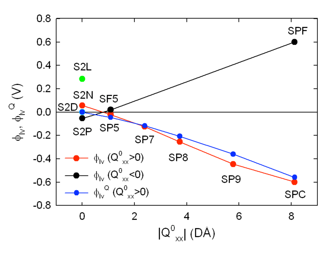
Figure 4: (Color on-line) Vapor-liquid interface potential drops for all studied models: standard (blue) and flipped (F)-charge (black) with respect to $|Q_{xx}^{0}|$ (molecular quadrupole moment).

Classical molecular dynamics (MD) simulations predict potentials on the order of $-0.5$ V for both vapor-liquid interfaces and membrane-liquid surfaces and, if used in the point ion approximation, $\Phi^{\prime}_{\rm pot}$, would seemingly yield the dominant contribution ($\sim 20~{}k_{\rm B}T$ for monovalent ions) to the PMF over a substantial part of the interfacial region 17 . This approximation, however, predicts incorrect results for the PMF and corresponding ion density, when compared with MD simulations, both in the infinitely dilute limit (as already pointed out in 17 ) and when incorporated into a modified Poisson-Boltzmann approach (to study higher electrolyte concentrations 16 ): neither the strong build-up of anions near a strongly hydrophobic uncharged surface (16 , Fig. 4a), nor the variations in the dilute limit of the PMF near a membrane surface (17 , Fig. 3) predicted by this approach are in agreement with MD simulations. This approximation also yields a very substantial, albeit seemingly undetected, direct contribution to the ionic free energy of solvation,

$$\Delta G^{\prime}_{0}=-\Phi^{\prime}_{\rm pot}(z_{v})=q\phi_{lv}.$$ (1)

on the order of $25~{}k_{\rm B}T$. Disturbingly, the reasonable agreement between the experimental results for the surface tension of electrolyte solutions and certain promising mesoscopic theoretical approaches that neglect the interface potential completely would be severely disrupted if such large interfacial potentials were taken into account 18 ; 18a . This situation becomes even more complicated if one considers that more “realistic” quantum mechanical calculations can lead to positive interface potentials of much higher amplitude (+3 eV) 11 ; 12 ; 13 , but no signature of such a potential is seen in recent ab initio simulations of ion solvation 14 .

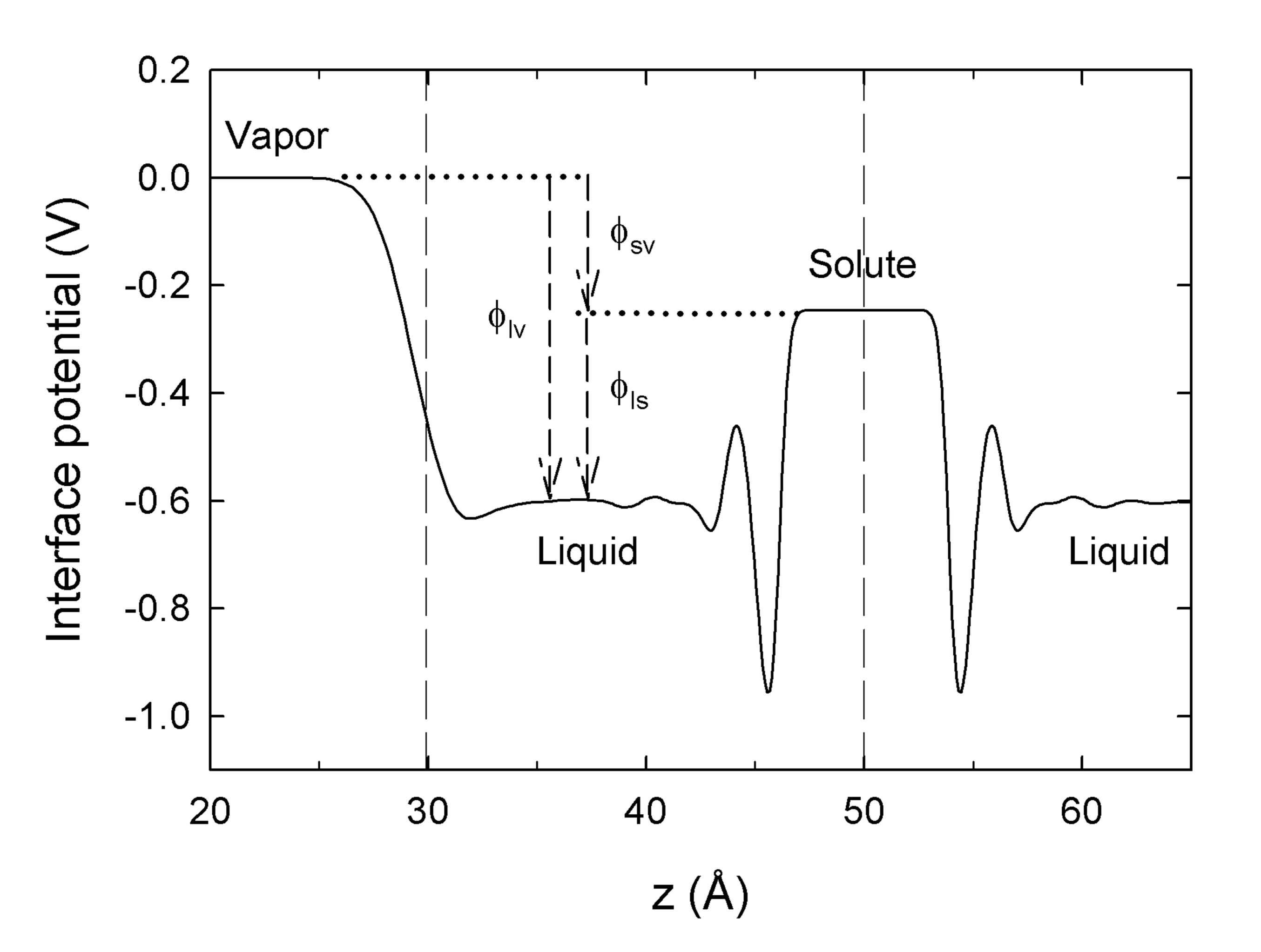
Figure 1: Electric potential variation, $\delta\phi(z)$, across the vapor-liquid and the liquid-solute interfaces for the neutral LJ solute I⁰ immersed in liquid water (SPC/E), at $z=50$ Å. The Gibbs dividing surface (GDS) of the macroscopic interface and the solute position are indicated by dashed vertical lines.

III Ionic free-energy of solvation

The electrostatic (ES) contributions to the total ion solvation free energy for the models studied here can be extracted directly from the MD simulations via

$$\Delta G_{\rm ES}^{\rm ion}=\Delta G_{0}+\Delta G_{\rm pol}$$ (2)

with

$$\Delta G_{0}=q\phi_{sv}=q(\phi_{lv}-\phi_{ls})$$ (3)

and

$$\Delta G_{\rm pol}\simeq q(\phi_{sv}^{\rm ion}-\phi_{sv})/2$$ (4)

where $\phi_{sv}=\phi_{s}-\phi_{v}=\phi_{lv}-\phi_{ls}$ and $\phi_{sv}^{\rm ion}=\phi_{lv}-\phi_{ls}^{\rm ion}$ are, respectively, the total vapor-liquid-solute potential variations for neutral and charged solutes. The ion solute-liquid interface potential, $\phi_{ls}^{\rm ion}=\phi_{l}^{\rm ion}-\phi_{s}^{\rm ion}$ is the potential difference between the bulk liquid and the center of the charged ion (with the bare Coulomb potential due to the ion itself subtracted out). The first, direct, term, $\Delta G_{0}=q\phi_{sv}$, may be regarded as the electrostatic free energy of solvation of an ion placed in the potential $\phi_{sv}$ created around its corresponding neutral counterpart; the second polarization term, $\Delta G_{\rm pol}$, obtained from an approximate generalized “charging” method 22 ; 23 , arises from the response of the solvent to the ion (which generates an overall potential variation $\phi_{sv}^{{\rm ion}}$ much larger in amplitude than $\phi_{sv})$ 23 . Because $\phi_{lv}$ is ion independent, the polarization contribution can be simplified to $\Delta G_{{\rm pol}}\simeq q(\phi_{ls}-\phi_{ls}^{\rm ion})/2$ and therefore be obtained from bulk simulations (this contribution is the microscopic analog of the mesoscopic Born one presented below). Since $(\phi_{ls}-\phi_{ls}^{\rm ion})\propto q$ vanishes in the limit $q\rightarrow 0$, $\Delta G_{{\rm pol}}\propto q^{2}$, as required for a polarization contribution (and also seen in the usual mesoscopic Born term below).

III.1 Mesoscopic Born model

Within the mesoscopic Born model, an ion is modeled as a point charge $q$ sitting in its spherical cavity of effective radius $R_{i}$ in bulk water treated as a continuum of dielectric constant $\varepsilon_{w}$. The radial electric potential around the central ionic charge, $\varphi_{\rm ion}(r)$, determines the Born approximation for the polarization contribution via

$$\Delta G_{\rm pol}^{\rm B}=\frac{q}{2}\mathop{\lim}\limits_{r\to 0}[\varphi_{\rm ion}(r)-\varphi_{0}(r)]=\frac{q^{2}}{8\pi\varepsilon_{0}R_{i}}\left(\frac{1}{\varepsilon_{w}}-1\right)$$ (5)

where $\varepsilon_{0}$ is the vacuum permittivity, $\varphi_{0}(r)$ is the bare Coulomb potential, and $\varepsilon_{w}\simeq 78$ is the dielectric constant of bulk water at room temperature. Although this type of polarization contribution ($\sim 100-180~{}k_{\rm B}T$) typically dominates the ionic solvation free energy for the ions studied here, it is neither clear how accurate the simple Born approximation is (due to the neglect of potentially important ion-solvent correlations near the ion), nor how to choose best $R_{i}$.

Furthermore, despite its dominant role in the global ionic free energy of solvation, the polarization contribution to the local ionic PMF, $\Phi(z)$, is seemingly not the dominant contribution over a significant part of the interfacial region, which means that the role of other contributions must be clarified 17 . Although a Born-type polarization term is commonly incorporated in mesoscopic approaches to the free energy of solvation (or PMF), the direct term, arising from the bare interfacial potential, is either completely neglected without justification 15 ; 18 ; 18a ; 19 or strongly overestimated by incorrectly assuming $\phi_{ls}=0$ in $\Delta G_{0}$ (eq. 3), which leads to the approximation $\Delta G^{\prime}_{0}=q\;\phi_{lv}$ (eq. 1) for the direct contribution [or $\Phi^{\prime}_{\rm pot}(z)$ in the PMF, which includes only the contribution of the vapor-liquid interface 17 ; 16 and neglects entirely that of the solute-liquid one] (see fig. 1).

IV Models and methods

We compare a direct evaluation from MD simulations of the two terms contributing to $\Delta G_{\rm ES}^{\rm ion}$, namely $\Delta G_{0}$ and $\Delta G_{\rm pol}$, for SPC/E water with the simplified approximations presented above, respectively, $\Delta G^{\prime}_{0}$ and $\Delta G_{{\rm pol}}^{\rm B}$. In order to shed further light on the interplay between the solvent molecular dipole and quadrupole moments (and thus water specificity), a series of molecular models having the same permanent dipole moment as SPC/E, but different quadrupolar ones, were first generated by reducing the H-O-H angle $\gamma$, while keeping fixed both the original partial charges on each site and the distance between the oxygen and the midpoint between hydrogen atoms. The choice of including the variable quadrupole moment models was dictated by the need to find a smooth link via MD simulations between a realistic water model (SPC/E) and the simplified purely dipolar models often studied (due to the inherent difficulty of the problem) using approximate theoretical methods 28a ; 28 . Due to symmetry the interfacial contributions under scrutiny here for liquids possessing molecular dipole and quadrupole moments must vanish for symmetric purely dipolar models. We also would like to test the approximate formulae for the quadrupolar contribution in a more general setting (from SPC/E to a purely dipolar model) and to shed light on the coupling between the dipolar and quadrupolar contributions. For all but one molecular model the SPC/E parameters were maintained for the Lennard-Jones (LJ) interaction centered on the oxygen atom. For the $n^{\rm th}$ molecule of each liquid model we define the molecular dipole moment $\mathbf{p}_{n}=\sum\nolimits_{j}q_{j}\mathbf{r}_{jn}$ and quadrupole moment tensor $(Q_{n})_{\alpha\beta}=3\sum\nolimits_{j}q_{j}x_{jn,\alpha}x_{jn,\beta}$, with $x_{jn,\alpha}$ the $\alpha^{\rm th}$ Cartesian component of the position vector $\mathbf{r}_{jn}$ of partial charge $q_{j}\;(j=1,2,3)$ with respect to the center of charges within molecule $n$. We can then compute the macroscopic polarization

$$\mathbf{P}(\mathbf{r})=\left\langle\sum\nolimits_{n}\mathbf{p}_{n}\delta(\mathbf{r}-\mathbf{r}_{n})\right\rangle$$ (6)

and the macroscopic quadrupole moment density,

$$Q_{\alpha\beta}(\mathbf{r})=\frac{1}{6}\left\langle\sum\nolimits_{n}(Q_{n})_{\alpha\beta}\delta(\mathbf{r}-\mathbf{r}_{n})\right\rangle$$ (7)

directly from the simulations as ensemble averages 2 .

The local electric charge density, $\rho(\mathbf{r})$, can be evaluated directly by extracting the partial charge density associated with the particular molecular model; and the associated electric field ${\bf{E}}$ and potential $\phi$ can then be obtained by integration of the Poisson equation in appropriate coordinates:

$$\nabla^{2}\phi=-\nabla\cdot{\bf{E}}=-\frac{\rho}{{\varepsilon_{0}}}.$$ (8)

The mean electric field along the direction normal to the planar vapor-liquid interface, at distance $z$ is written in Cartesian coordinates as:

$$E_{z}\left(z\right)=\int\limits_{z_{v}}^{z}{\frac{{\rho\left({z^{\prime}}\right)}}{{\varepsilon_{0}}}dz^{\prime}},$$ (9)

where $\rho\left({z^{\prime}}\right)$ represents the average electric charge density (evaluated within the scope of MD simulations as the volume density of the sum of partial charges associated with a particular molecular model found in the bin corresponding to the position $z^{\prime}$). The coordinate $z_{v}$ is the origin of integration in the vapor phase (far from the interface). Similarly, in spherical coordinates (appropriate for the curved solute-liquid interface), the mean electric field is given by

$$E_{r}\left(r\right)=\frac{1}{r^{2}}\int\limits_{0}^{r}{\frac{{\rho\left({r^{\prime}}\right)r^{\prime 2}}}{{\varepsilon_{0}}}dr^{\prime}}.$$ (10)

The total charge density can also be expressed as a multipole expansion jack ,

$$\rho=-\nabla\cdot{\bf{P}}+\sum_{\alpha,\beta}\nabla_{\alpha}\nabla_{\beta}Q_{\alpha\beta}+\ldots,$$ (11)

here truncated after the quadrupolar term. The dipolar and quadrupolar electric fields and potentials can then be obtained from the dipole moment density ${\bf{P}}$ and quadrupole moment density $Q$, respectively:

$$\nabla^{2}\phi^{D}=-\nabla\cdot{\bf{E}}^{D}=\frac{1}{\varepsilon_{0}}\nabla\cdot{\bf{P}}=-\frac{1}{\varepsilon_{0}}\rho^{D}$$ (12)

$$\nabla^{2}\phi^{Q}=-\nabla\cdot{\bf{E}}^{Q}=-\frac{1}{\varepsilon_{0}}\sum_{\alpha,\beta}\nabla_{\alpha}\nabla_{\beta}Q_{\alpha\beta}=-\frac{1}{\varepsilon_{0}}\rho^{Q}$$ (13)

After computing the full interface potential from eq. 8, we compare it with the sum of the dipolar and quadrupolar contributions computed from eqs. 12 and 13 to assess the accuracy of the truncated multipole expansion.

The dipolar contribution to the total electric field can be obtained from $\rho^{D}=-\nabla\cdot{\bf{P}}$, the mean dipolar charge density created by the distribution of the macroscopic dipole moment density ${\bf{P}}$, yielding for the $z$-component:

$$E_{z}^{D}\left(z\right)=-\frac{{P_{z}\left(z\right)}}{{\varepsilon_{0}}},$$ (14)

since $P_{z}$ vanishes at $z_{v}$ in the vapor phase, far from the interface region. Similarly, the dipolar component of the radial field in spherical coordinates, appropriate for the solute-liquid interface, reads:

$$E_{r}^{D}\left(r\right)=-\frac{{P_{r}\left(r\right)}}{{\varepsilon_{0}}},$$ (15)

where $P_{r}\left(r\right)$ represents the radial distribution of the density of the dipole moment. The dipole moment density ${\bf{P}}$ obtained from the MD simulations as ensemble averages of molecular dipole moments is presented in detail below for the planar l-v interface (Section V.1).

The determination of the mean electric field (or charge density) permits the calculation of $\delta\phi\left(z\right)=\phi\left(z\right)-\phi\left({z_{v}}\right)$, the local electric potential difference evaluated at position $z$ in the vicinity of the interface:

$$\delta\phi\left(z\right)=-\int\limits_{z_{v}}^{z}{E_{z}\left({z^{\prime}}\right)dz^{\prime}}={\frac{1}{{\varepsilon_{0}}}\int\limits_{z_{v}}^{z}{\rho\left({z^{\prime}}\right)\left({z^{\prime}-z}\right)}\,dz^{\prime}}$$ (16)

Similarly, the dipolar local potential profiles, $\delta\phi^{D}\left(z\right)$, can be obtained from the corresponding electric field, $E_{z}^{D}\left(z\right)$ (or charge density, $\rho^{D}$).

The quadrupole moments of the models SPC, SP9-SP5, and S2N range from the SPC/E value down to zero (table 1). Because both dipolar S2N and S2L models are asymmetric, a symmetric dumbbell-like model (S2D) was also investigated (with two LJ spheres on both ends of the dipole). Ions are modeled as simple point charges carrying an LJ sphere.

Table 1: The system parameters [$\gamma$ is the H-O-H angle; $\mu^{0}$ and $Q^{0}_{xx}$ are the permanent molecular dipole and quadrupole moments; $\rho_{l}$ is the liquid density at the center of the slab (estimated error of $\pm 0.005$ g/cm³)], total interfacial potential $\phi_{lv}$, the corresponding quadru- ($\phi_{lv}^{Q}$) and dipolar ($\phi_{lv}^{D}$) contributions, and the “isotropic” quadrupolar approximation ($\phi_{lv,{\rm est}}^{Q}$, eq. 19); Estimated standard error of $\pm 0.5$ mV for the vapor-liquid interface potentials of the studied liquid models (obtained using the block averaging method).

Model	$\gamma(^{\circ})$	$\mu^{0}$(D)	$Q_{xx}^{0}$(DÅ)	$\rho_{l}$(g/cm3)	$\phi_{lv}$(mV)	$\phi_{lv}-\phi_{lv}^{D}$(mV)	$\phi_{lv}^{Q}$(mV)	$\phi_{lv,{\rm est}}^{Q}$(mV)	$\phi_{lv}^{Q}/\phi_{lv}$
SPC	109.5	2.347	8.131	0.981	-600.3	-558.8	-559.2	-558.6	0.932
SP9	100.0	2.347	5.775	0.892	-445.8	-361.4	-360.1	-360.2	0.808
SP8	87.6	2.347	3.736	0.787	-254.8	-206.5	-206.8	-205.9	0.811
SP7	75.0	2.347	2.394	0.698	-123.6	-116.1	-116.9	-117.1	0.946
SP5	54.7	2.347	1.089	0.611	-21.4	-46.3	-46.2	-46.6	–
S2N	0	2.347	0	0.556	56.8	0.2	0	0	0
S2L	0	4.065	0	0.696	284.6	-0.4	0	0	0
S2D	0	2.347	0	0.658	-0.8	-0.4	0	0	0

Simulations of the vapor-liquid interface were carried out using a modified parallel version of the molecular dynamics package Amber 9 amber and a slab geometry methodology similar to the one often used in the literature: 1000 liquid molecules placed in a rectangular unit cell of dimensions 31.04 $\times$ 31.04 $\times$ 91.04 ų occupying roughly the middle one-third of the available space and generating two vapor-liquid interfaces 24 ; 24a . A Lennard-Jones interaction potential is centered on the solvant oxygen atom, characterized by the SPC/E parameters $\sigma=3.1657$ Å  and $\varepsilon=0.1553$ kcal/mol. In the “bulk” ion solvation simulations, the system comprised a cubic cell of 1000 water molecules, with one solute immersed at its center.

The ion properties are summarized in table 2. Each ion is modeled by a simple point charge, a Lennard-Jones potential defined by $\sigma$ and $\varepsilon$ and, when polarizable models are analyzed, a polarizability. The cross parameters for the ion-water Lennard-Jones interaction are determined via Lorentz-Berthelot mixing rules.

Table 2: Lennard-Jones parameters $\sigma$ and $\varepsilon$, and polarizability $\alpha$ for ions

Ion	$q$ ($e$)	$\sigma$ (Å)	$\varepsilon$ (kcal/mol)	$\alpha$	ref.
Na+	1	2.350	0.13	0.24	24a1
F-	-1	3.168	0.2	0.974	24a2
Cl-	-1	4.339	0.1	3.25	24a3
Br-	-1	4.700	0.1	4.53	24a4
I-	-1	5.150	0.1	6.9	24a4

Periodic boundary conditions were applied in all three directions. The long-range charge-charge, charge-dipole and dipole-dipole interactions were treated by the particle-mesh Ewald summation method for both the charge and dipole moments 24b . For computational efficiency, in the polarizable simulations, an extended Lagrangian method was utilized to compute the induced dipole moments, regarded as additional dynamic variables 24c .

A cutoff radius of 10 Å was used for the short-ranged non-bonded LJ interactions and for the real space component of the Ewald summation. The geometries of the liquid molecules were constrained by applying the SHAKE algorithm with a relative geometric tolerance of $10^{-4}$. The equations of motion were integrated using the velocity Verlet algorithm with a default time step of 1 fs 24d . In order to avoid occasional drifts of the slab along the z-axis normal to the interface, the center-of-mass (COM) velocity was removed every 1000 steps. Configurations were saved every 100 fs in the output trajectories and each such frame was readjusted with respect to the z-axis, to keep the COM of the electrolyte fixed relative to the simulation cell.

Starting from the initial configuration of each simulated system, an energy minimization was performed, followed by a 1 ns NVT equilibration at 300 K for the slab systems. For simulations of bulk water ion solvation the equilibration process was performed in the NPT ensemble, using a weak-coupling pressure regulation with a target pressure of 1 bar. Subsequently, in both cases, at least 5 ns of measurements in the NVT ensemble were carried out, using the Berendsen thermostat with the configurational degrees of freedom coupled to a heat bath with coupling constant $\tau=1$ ps 24e . In the special case of polarizability-enabled simulations, the degrees of freedom related to the induced dipole moment of the ion were independently coupled to a 1 K heat bath (relaxation time $\tau_{\rm dip}=10$ ps), ensuring a proper handling of the electronic degrees of freedom 24f . All computed profiles spanning the vapor-liquid interface were obtained as ensemble averages of the instantaneous profiles evaluated in thin slabs (bins) of thickness 0.2 Å parallel to the interface. For the radial quantities measured in the bulk simulations of ion solvation, equally distanced, 0.1 Å thick, spherical shell bins have been employed. Due to the cubic dimensions of the simulation box the radial profiles are relevant up to approximately 15 Å.

V MD simulation results

The MD simulation results show that the bulk region density decreases with decreasing molecular quadrupole moment (at constant dipole moment), varying by nearly a factor of two in going from SPC/E to the lowest density model, S2N (table 1). For the models possessing quadrupole moments, SPC/E – SP5, the density decreases by less than 40%, despite a decrease by a factor of 8 in the molecular quadrupole moment. This density variation is an expected physical consequence of the reduction in water coordination as the molecular quadrupole moment decreases. The S2N and S2L models form purely dipolar liquids with a characteristic chain-like structure arising from the head-to-tail alignment of the dipole moments and a lower bulk density due to the decrease in hydrogen bond coordination from four to two. The vapor-water interfacial thickness is found to be approximately 3.8 Å at 300 K for SPC/E and increases along with the slab thickness as the molecular quadrupole moment decreases.

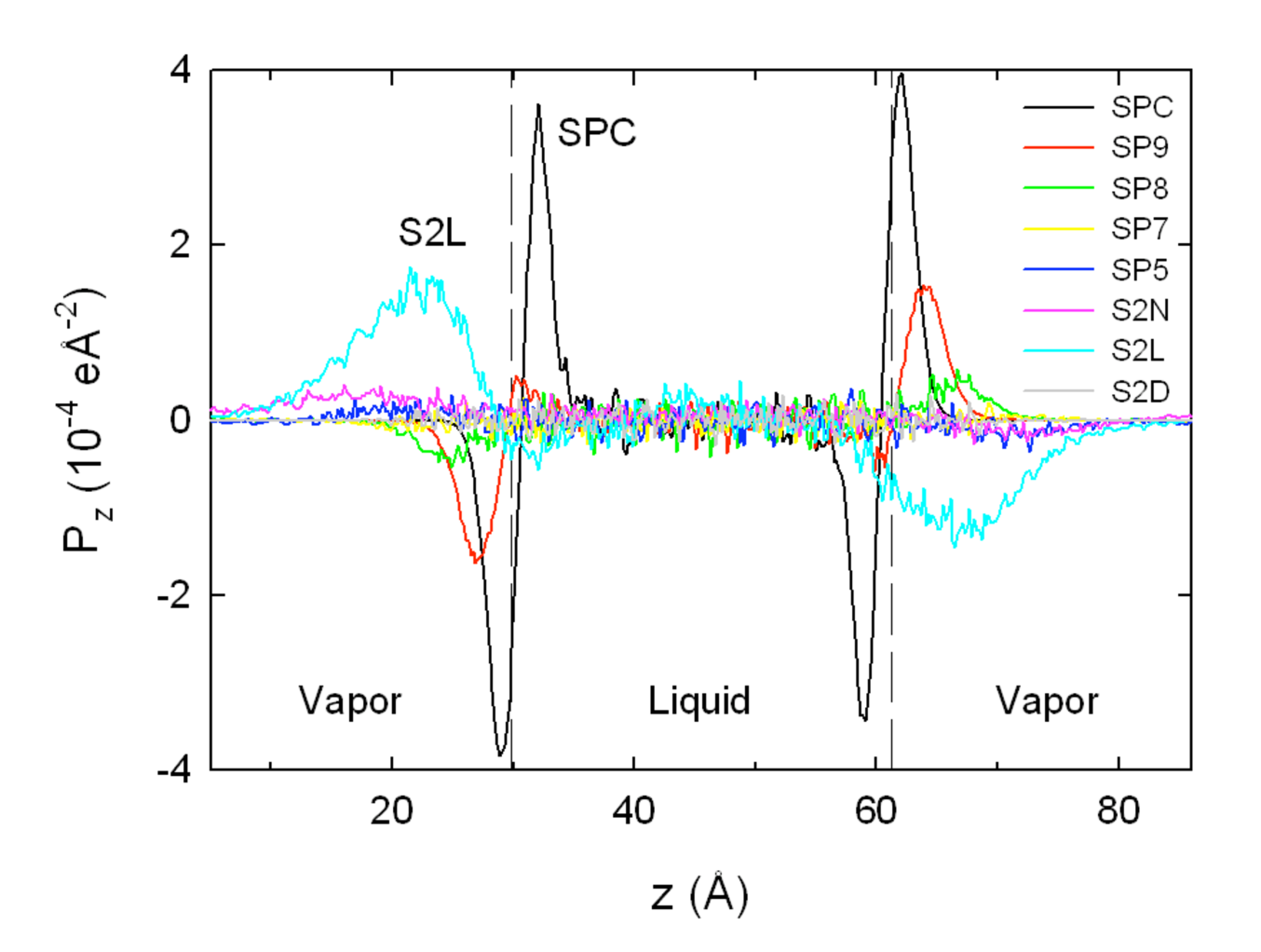
Figure 2: (Color on-line) The dipole moment density, $P_{z}(z)$, for all studied liquids at the vapor-liquid interface. Dashed vertical lines represent the GDS of both interfaces for SPC/E.

V.1 Dipolar ordering

Orientational (dipolar) ordering of water takes place near the l-v interface, which can be seen by plotting $P_{z}(z)$ for the series of model liquids (fig. 2). Orientational double layers were found only for SPC/E and SP9 with the outer layer dipoles pointing preferentially towards the vapor phase and in the opposite direction in the inner layers (closest to the slab center). For models with lower molecular quadrupole moments the molecular dipoles point towards the liquid phase. Because of the asymmetry created by the oxygen LJ sphere, asymmetric purely dipolar liquids (S2N and S2L) still possess orientational ordering in the interface region due to the hydrophobic forces tending to exclude the oxygen LJ sphere from the liquid slab.

V.2 Vapor-liquid interface potential: multipole contributions

In order to illustrate how various multipole moments contribute to the vapor-liquid interface potential, we obtained the electric potential difference by integration of the Poisson equation from the charge density obtained from the first two terms of the multipole expansion 2 ; 10 ,

$$\rho(z)\approx\rho^{D}(z)+\rho^{Q}(z)=-\frac{d}{{dz}}\left[{P_{z}\left(z\right)-\frac{d}{{dz}}Q_{zz}\left(z\right)}\right]$$ (17)

leading to the first two (dipolar and quadrupolar) contributions to the interface potential:

$$\delta\phi^{DQ}(z)\equiv\delta\phi^{D}(z)+\delta\phi^{Q}(z)=\int_{z_{v}}^{z}\frac{P_{z}(z)}{\varepsilon_{0}}dz-\frac{Q_{zz}(z)}{\varepsilon_{0}}$$ (18)

since $Q_{zz}$ is taken to vanish in the vapor phase and $P_{z}$ vanishes in both bulk (vapor and liquid) phases. For the planar interface higher order moments do not contribute.

The “exact” model interface potential profile and the corresponding dipolar and quadrupolar contributions (eq. 18) obtained directly from the simulation data (using, respectively, the “exact” partial charge density, $\rho$, and the multipole contributions of eq. 17) are illustrated in fig. 3. The total vapor-liquid potential reaches $-600$mV for SPC/E, in agreement with previous values 5 , but decreases in amplitude with decreasing molecular quadrupole moment (SP9 to SP5). The asymmetric purely dipolar liquids, on the other hand, have positive interface potentials, whereas, as expected by symmetry considerations, the fully symmetric model S2D gives a null result (table 1). The two components of the interface potential reveal very different types of profiles with the quadrupolar potential being negative, as expected for models with positive molecular quadrupole moments. For the SPC/E model the quadrupolar contribution represents more than 90% of the total. This contribution decreases rapidly with decreasing molecular quadrupolar moment and becomes comparable in absolute value with the (positive) dipolar contribution for SP5, the near cancellation in this case leading to a very low (negative) total value. For SPC/E, SP9-SP7 the quadrupole contribution provides the major contribution to the interface potential (figs. 3 and 4, table 1) and thus to the large interfacial electric fields ($\sim 1$ V/nm for SPC/E) directed towards the liquid phase over a substantial part of the interfacial region 23 . For SPC/E and SP9 the innermost dipoles tend to follow this field, creating in turn an opposing dipolar field that acts to align the outermost molecular dipoles in the opposite direction. Although the quadrupolar potential profile is always monotonic, the dipolar one shows a minimum close to the Gibbs dividing surface (GDS) for both SPC/E and SP9 models due to the dipolar orientational bilayers. These results reveal a subtle interplay between the dominant quadrupolar contribution and the dipolar response.

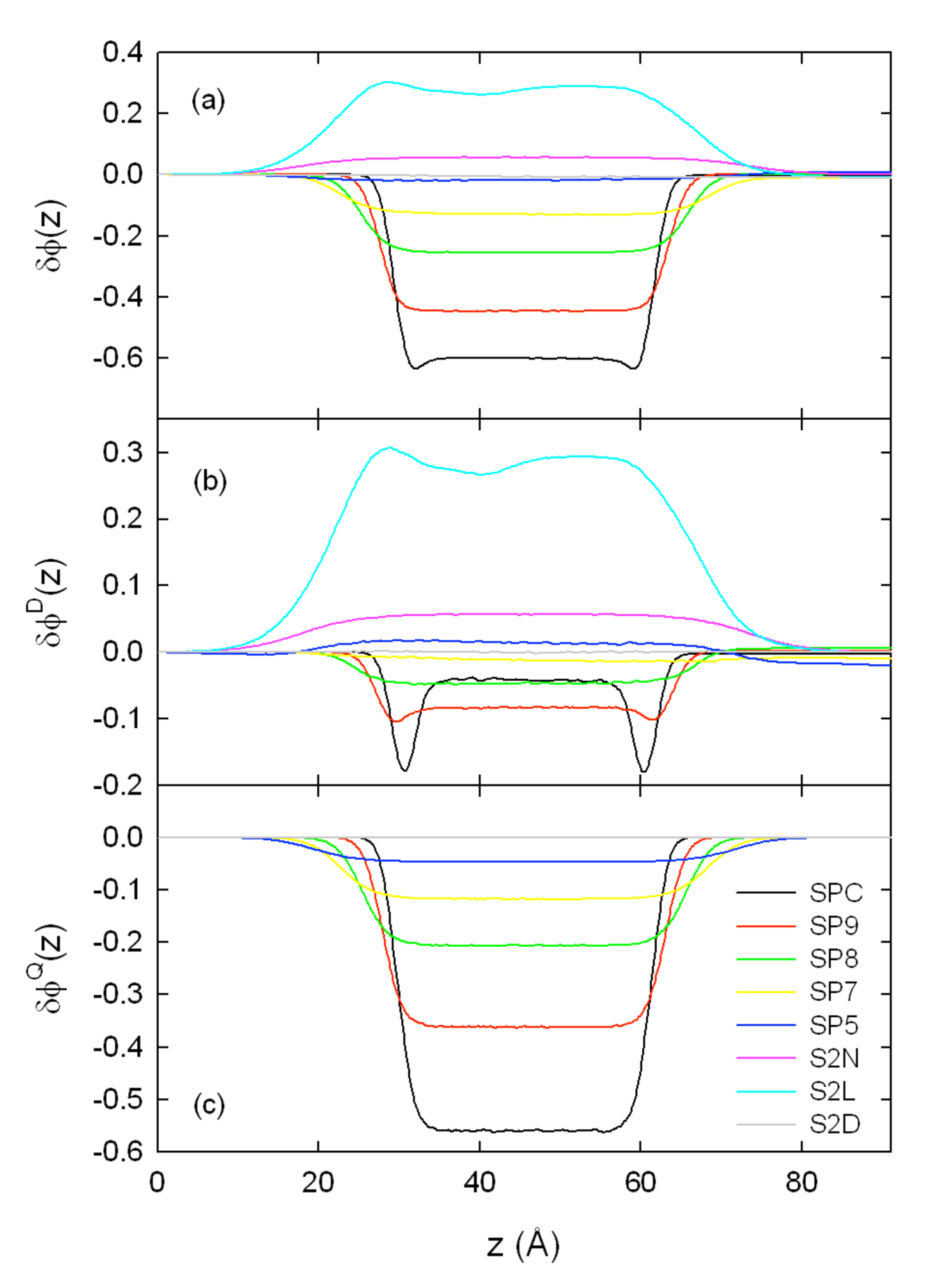
Figure 3: (Color on-line) (a) Total, (b) dipolar and (c) quadrupolar potential profiles, $\delta\phi(z)$ (in volts) for the studied liquids characterized by positive molecular quadrupolar moments.

Even if the system is not isotropic in the interfacial region, it is possible to generalize the approach presented in 2 ; 10 ; 13 to construct a simple but extremely accurate “isotropic” approximation for the quadrupolar contribution to the local vapor-liquid interface potential using only the water density profile and the molecular quadrupole moment $Q^{0}$ evaluated in a local reference frame with the $y$-axis along the dipole vector and the $z$-axis out of the molecular plane:

$$\delta\phi_{\rm est}^{Q}(z)=-\frac{c(z)}{6\varepsilon_{0}}\frac{{\rm Tr}\;Q^{0}}{3},$$ (19)

where $c(z)$ is the local liquid number density taken from the simulations. In this reference frame the only non-zero component is $Q^{0}_{xx}$ and therefore in this case ${\rm Tr}\;\textsf{Q}^{0}=Q_{xx}^{0}$. The estimate $\phi_{lv,{\rm est}}^{Q}=\delta\phi_{\rm est}^{Q}(z_{l})$ for the quadrupolar contribution is in excellent agreement with direct determinations (table 1). We see from eq. 19 that the variations in vapor-liquid interface potentials for the models with non-zero quadrupole moments are mainly determined by the quadrupolar contribution and therefore dominated by the variations in the molecular quadrupole moments (with the physically relevant density variations playing only a secondary role). For this reason and because the dipolar contribution is not strictly proportional to the liquid density, we do not attempt to normalize the vapor-liquid interface potentials in table 1 to correct for the variations in liquid density. We have also checked that this simple quadrupolar estimation 19 provides a very good approximation to the full oscillatory membrane-water surface potential 17 , confirming that the air-water interfacial and membrane-water surface potentials are mainly determined by the local water density and molecular quadrupole moment. Furthermore, we propose that this method can be used to estimate the quadrupolar potential contribution of any liquid, irrespective of its bulk molecular quadrupole moment, even those obtained from ab initio quantum mechanical calculations of liquid water. As an illustration, we have checked that when ab initio values for ${\rm Tr}\;\textsf{Q}^{0}$ 29a ; 24g , are injected into the simple approximation Eq. 19, we find quadrupolar potentials in reasonable agreement with the (quadrupole dominated) total interface potentials (+3 eV) extracted directly from the quantum mechanical calculations 12 ; 13 .

V.3 Solute-Liquid interface potential

In the presence of a solute the planar vapor-liquid interface potential has as counterpart the microscopic potential between the solute center and the surrounding liquid (of which the first two multipole terms can be obtained from the microscopic analog of eq. 18 23 ).

The local radial solute-liquid potential profile, defined as

$$\delta\phi_{r}\left(r\right)=\phi_{r}\left(r\right)-\phi_{r}\left({r_{s}}\right)$$ (20)

[with $\phi_{r}\left({r_{s}}\right)=0$ at the center of the solute $r_{s}=0$], is obtained from the radial charge density $\rho_{r}\left(r\right)$ by integrating the Poisson equation (8) in spherical coordinates:

$$\delta\phi_{r}\left(r\right)=-\int\limits_{0}^{r}E_{r}(r^{\prime})dr^{\prime}=-\int\limits_{0}^{r}{\frac{{\rho_{r}\left({r^{\prime}}\right)\left({r^{\prime}}\right)^{2}}}{{\varepsilon_{0}}}\left({\frac{1}{{r^{\prime}}}-\frac{1}{r}}\right)dr^{\prime}}.$$ (21)

The dipolar component, $\delta\phi_{r}^{D}\left(r\right)$, is determined from the dipole moment density $P_{r}\left(r\right)$ as:

$$\delta\phi_{r}^{D}\left(r\right)=\int\limits_{0}^{r}{\frac{{P_{r}\left({r^{\prime}}\right)}}{{\varepsilon_{0}}}dr^{\prime}}$$ (22)

The corresponding radial electric fields, $E_{r}\left(r\right)$ and $E_{r}^{D}\left(r\right)$, are determined from equations (10) and (15).

The quadrupolar contribution to the total radial interface potential, $\delta\phi_{r}^{Q}\left(r\right)$ is accessible from the simulation data via the radial dependence of the quadrupole moment density written in spherical coordinates, $\textsf{Q}^{\prime}(r)$. We begin by writing the quadrupolar Poisson equation (13) in Cartesian coordinates (centered at the solute position $r_{s}=0$), with the tensor elements of the Cartesian quadrupole moment density, $Q_{\alpha\beta}$:

$$\varepsilon_{0}\nabla\cdot{\bf{E}}^{Q}=\sum\limits_{\alpha,\beta}{\nabla_{\alpha}\nabla_{\beta}Q_{\alpha\beta}}$$ (23)

Using the divergence theorem, we find:

$$\varepsilon_{0}\mathop{{\int\!\!\!\!\!\int}\mkern-21.0mu\bigcirc}\limits_{S}{\bf{E}^{Q}\cdot d{\bf{S}}}=\mathop{{\int\!\!\!\!\!\int}\mkern-21.0mu\bigcirc}\limits_{S}{\sum\limits_{\alpha,\beta}{\nabla_{\alpha}Q_{\alpha\beta}}\cdot n_{\beta}dS},$$ (24)

where $\hat{\bf{n}}$ is the normal to the interface. Letting $F_{\beta}=\sum\limits_{\alpha}{\nabla_{\alpha}Q_{\alpha\beta}}$ and $S=4\pi r^{2}$, we obtain the radial dependence of the quadrupolar electric field $E_{r}^{Q}\left(r\right)$, by integrating over the angular degrees of freedom:

$$4\pi\varepsilon_{0}E_{r}^{Q}\left(r\right)=\mathop{{\int\!\!\!\!\!\int}\mkern-21.0mu\bigcirc}\limits_{S}{F_{r}\sin\theta d\theta d\phi},$$ (25)

with $F_{r}=\bf{e}_{r}\cdot\bf{F}$ (where $\bf{e}_{r}$ is the unit radial vector). After performing the angular integrals, we obtain the radial dependence of the quadrupolar electric field:

$$\varepsilon_{0}E_{r}^{Q}\left(r\right)=\frac{{\partial Q^{\prime}_{rr}}}{{\partial r}}+\frac{1}{r}\left({3Q^{\prime}_{rr}-TrQ}\right).$$ (26)

Since $E_{r}^{Q}\left(r\right)=-\frac{{\partial\phi_{r}^{Q}\left(r\right)}}{{\partial r}}$ and $\phi_{r}^{Q}\left(0\right)=0$, we arrive at the final solution for the local quadrupolar potential at position $r$, with respect to the center of the solute, $\delta\phi_{r}^{Q}=\phi_{r}^{Q}\left(r\right)-\phi_{r}^{Q}\left({r_{s}}\right)$, in terms of two components:

$$\delta\phi_{r}^{Q}(r)=\delta\phi_{r}^{Q,1}(r)+\delta\phi_{r}^{Q,2}(r)$$ (27)

with

$$\delta\phi_{r}^{Q,1}\left(r\right) = -\frac{1}{\varepsilon_{0}}Q^{\prime}_{rr}\left(r\right)$$ (28)

$$\delta\phi_{r}^{Q,2}\left(r\right) = \frac{1}{\varepsilon_{0}}\int\limits_{0}^{r}\frac{dr^{\prime}}{{r^{\prime}}}\left[{\rm Tr}\textsf{Q}({r^{\prime}})-3Q^{\prime}_{rr}({r^{\prime}})\right].$$ (29)

The second contribution is generated by the symmetry breaking of the diagonal components of $\textsf{Q}^{\prime}$ in the solute-liquid interfacial region. The detailed calculations leading from $\textsf{Q}\left({\bf{r}}\right)$ to $\delta\phi_{r}^{Q}\left(r\right)$ will be presented elsewhere 23 . Far from the solute center the radial solute-liquid interface potential and the various multipole components tend to their respective asymptotic values: $\phi_{ls}=\delta\phi_{r}(\infty)$, $\phi_{ls}^{D}=\delta\phi_{r}^{D}(\infty)$, and $\phi_{ls}^{Q}=\delta\phi_{r}^{Q}(\infty)$.

Because the solute-liquid interface is curved, the associated potential depends on the size of the cavity and is therefore ion specific. Thus, there is a first potential drop when going from the vapor into the liquid phase, followed by an overall increase near the solute, yielding a smaller, overall negative, vapor-liquid-solute potential drop, $\phi_{sv}$ (fig. 1). To obtain a fuller picture, we have extracted the solute-liquid interfacial potentials (and the dipolar/quadrupolar components) from MD simulations of neutral ion-like solutes, fixed at the center of a cubic box of bulk SPC/E water (using eqs. 21, 22,and 27). The solute-liquid potential $\phi_{ls}$ and the corresponding dipolar contribution $\phi_{ls}^{D}$ are obtained, respectively, from the radial charge density and the dipole moment density distributions. The higher order multipole contributions, $\phi_{ls}-\phi_{ls}^{D}$, are dominant and, due to ls interface curvature effects, not only is the amplitude of the ls quadrupolar contribution different from the lv one, but multipole terms beyond the quadrupolar one play a non-negligible role (tables 3 and 4) 23 . For the halide-like neutral solutes $\phi_{ls}$ decreases in amplitude with increasing solute size and is smaller than for the neutral sodium like solute, Na⁰. For I⁰, $\phi_{ls}$ increases in amplitude by about 6% when the polarizability is turned on. Although the $\phi_{ls}^{Q,1}$ contribution is dominant in $\phi_{ls}$, it simply serves, as we shall see below, to cancel the large vapor-liquid quadrupolar contribution to the direct contribution to the free energy of ion solvation, $\Delta G_{0}$. The dipole contribution $\phi_{ls}^{D}$ goes from negative values for small halide-like solutes (F⁰) to positive values for larger ones.

V.4 Free energy of ion solvation

The solute-liquid potential was then used to evaluate the direct contribution to the free energy of ion solvation, $\Delta G_{0}=q(\phi_{lv}-\phi_{ls})$ (eq. 3), dominated by the difference between the quadrupolar lv and ls contributions, which do not cancel due to strong curvature effects for the small ions under study. Because the $\phi_{ls}^{Q,1}$ component depends only on the bulk solvent properties, it is in principle equal to $\phi_{lv}^{Q}$ and therefore the two terms should cancel in $\Delta G_{0}$, leaving the dominant ion specific quadrupolar contribution, $\phi_{ls}^{Q,2}$ (tables 3 and 4). The dipolar contribution and multipolar contributions higher than quadrupolar play non-negligible, but secondary roles, in $\Delta G_{0}$. Our results for polarizable $I^{-}$ also reveal that ionic polarizability plays a minor but non-negligible role in determining $\Delta G_{0}$ (tables 3 and 4).

Table 3: Solute-liquid interface potentials with multipolar contributions for neutral solutes solvated in SPC/E water (for which the vapor-liquid interface potential is $\phi_{lv}=-600.3$ mV with $\phi_{lv}^{Q}=-559.2$ mV and $\phi_{lv}^{D}=-41.5$ mV). In principle $\phi_{ls}^{Q,1}=\phi_{lv}^{Q}$. The less than 2% difference between the values obtained from the water slab and bulk simulations can be attributed to the differences in densities generated by the finite slab thickness and the barostat used in the NPT bulk simulations (cf. eq 19). To directly compare solute-liquid and vapor-liquid interface potentials, we correct for this small systematic liquid density difference by defining a solute-dependent rescaled vapor-liquid interface potential, $\phi_{lv}^{*}=C\phi_{lv}$, where $C\equiv\phi_{ls}^{Q,1}/\phi_{lv}^{Q}$ (rescaled multipole vapor-liquid interface components are defined similarly). The estimated standard error for the interface potentials is 0.15 mV and pol denotes polarizable.

Solute	$\phi_{ls}/\phi_{lv}^{*}$ (%)	$\phi_{ls}$(mV)	$\phi_{ls}^{D}$ (mV)	$\phi_{ls}^{Q}$ (mV)	$\phi_{ls}^{Q,1}$ (mV)	$\phi_{ls}^{Q,2}$ (mV) )	$\phi_{ls}-\phi_{ls}^{D}-\phi_{ls}^{Q}$(mV)
Na0	66.7	-405.7	-78.8	-423.6	-566.7	143.1	96.7
F0	62.4	-380.0	-41.6	-415.3	-567.3	152.0	76.9
Cl0	60.3	-369.0	0.3	-426.8	-569.9	143.1	57.5
Br0	58.8	-359.8	17.8	-430.8	-569.6	138.8	53.2
I0	58.4	-357.5	32.3	-437.6	-570.5	132.9	47.8
I0 (pol)	62.1	-380.1	14.4	-440.0	-570.5	130.5	45.5

Table 4: Comparison of the different multipole contributions to the direct electrostatic solvation-free energies, $\Delta G_{0}^{*}=q(\phi_{lv}^{*}-\phi_{ls})$, obtained using the rescaled vapor-liquid interface potentials (*), of various ions as obtained directly from the simulations (see table 2) ($\Delta{G}^{\prime}_{0}\simeq\pm 0.6003$ eV); estimated errors: 0.002 eV

.

Solute	$\Delta G_{0}^{*}$ (eV)	Dipole∗ (%)	Quadrupole∗ (%)	Higher order∗ (%)
Na+	-0.2030	-18.1	70.5	47.6
F-	0.2294	0.2	66.3	33.5
Cl-	0.2432	17.5	58.8	23.6
Br-	0.2521	23.8	55.1	21.1
I-	0.2554	29.2	52.0	18.8
I- (pol)	0.2327	24.4	56.0	19.6

Table 5: Comparison of electrostatic solvation-free energies for various ions as obtained directly from the simulations, $\Delta G_{{\rm ES}}^{{\rm ion}}=\Delta G_{0}+\Delta G_{{\rm pol}}$, with the estimate $\Delta G_{{\rm ES,est}}^{{\rm ion}}=\Delta{G}^{\prime}_{0}+\Delta G_{{\rm pol}}^{\rm B}$ obtained from the truncated direct contribution [$\Delta{G}^{\prime}_{0}\simeq\pm 0.6$ eV for monovalent anions (resp. cations)] and the Born approximation, $\Delta G_{\rm pol}^{\rm B}$ . $R_{i}$ is chosen as the distance from the ion center where the ion-water radial distribution functions first reach 1 23 . To correct for the small systematic differences in liquid density between water slab and bulk simulations, the rescaled vapor-liquid interface potentials, $\phi_{lv}^{*}$, are used in the evaluation of the direct contribution: $\Delta G_{0}^{*}=q(\phi_{lv}^{*}-\phi_{ls})$ (see table 3). Estimated error of 0.025Å for $R_{i}$; Estimated standard errors: 0.002 eV for $\Delta G_{0}$; 0.05 eV for the other solvation-free energies. (1 eV$=23.06$ kcal/mol$\simeq 40k_{\rm B}T$)

Solute	$R_{i}$ (Å)	$\Delta G_{0}^{*}$ (eV)	$\Delta G_{\rm pol}^{\rm B}$ (eV)	$\Delta G_{\rm pol}$ (eV)	$\Delta G_{\rm ES,est}^{\rm ion}$ (eV)	$\Delta G_{\rm ES}^{\rm ion}$ (eV)	$\Delta G_{\rm exp}^{\rm ion}$ (eV) 29a
Na-	1.05	0.2030	-6.76	-6.88	-6.57	-6.68	–
F-	1.55	0.2294	-4.58	-4.46	-4.36	-4.23	-4.50
Cl-	2.00	0.2432	-3.55	-3.34	-3.32	-3.10	-3.64
Br-	2.25	0.2521	-3.15	-3.01	-2.91	-2.76	-3.30
I-	2.45	0.2554	-2.90	-2.63	-2.66	-2.38	-2.90
Na+	2.20	-0.2030	-3.23	-3.88	-3.42	-4.08	-4.26
I+	3.55	-0.2554	-2.00	-1.79	-2.24	-2.04	–

The key point is that $\Delta G_{0}$ is much smaller in amplitude than the simple direct estimate ($|\Delta G^{\prime}_{0}|=0.600$ eV) because of the strong partial cancellation of the two interface potentials, $\phi_{lv}$ and $\phi_{ls}$. Our results show that the direct contribution, $\Delta G_{0}$ is reduced to 30-40% of the simple direct estimate $\Delta G^{\prime}_{0}$ and depends on the sign of the ion charge in such a way as to favor the solvation of cations Na⁺ with respect to the anions (halogens). For the halogens $\Delta G_{0}$ is positive and increases with increasing ion size, thus augmenting the interface propensity of large anions like I^-. Because the amplitude of $\Delta G_{0}$ ($\sim\,0.20-0.26$ eV) is still between 5% (for F^-) and 10% (for I^-) of the dominant polarization contribution, $\Delta G_{\rm pol}$ (see table 5), it is on par with other important contributions (such as the hydrophobic one 16 ; 18 ; 18a ; 19a ; 25 ) and therefore must be taken into account correctly when considering ion-specific effects.

Because of charge-dipole and charge-quadrupole coupling, when the ion charge is “turned on” the solvent molecules reorient themselves in order to accommodate the solute, optimizing as much as possible the orientation and number of hydrogen bonds: the ion polarizes the medium around it and induces a radial potential difference, $\phi_{ls}^{\rm ion}$, dominated by the “long range” dipolar contribution. The difference between $\phi_{ls}^{\rm ion}$ and $\phi_{ls}$ extracted from the simulations then determines $\Delta G_{\rm pol}$ (eq. 4). With our choice of effective ion radius, the simple mesoscopic Born approximation $\Delta G_{\rm pol}^{\rm B}$ is in reasonably good agreement with the microscopic polarization contribution, $\Delta G_{\rm pol}$ (table 5). The polarization contribution to the solvation free energy, which is the main effect favoring high ion solvation, decreases in amplitude with increasing halogen size. We note also that the simulation results for the electrostatic contribution to the ionic free energy of solvation, $\Delta G_{\rm ES}^{\rm ion}$, follow the experimental trend, $\Delta G_{\rm exp}^{\rm ion}$, reasonably well (table 5), despite the neglect of certain entropic (hydrophobic) and enthalpic contributions (arising, for example, from the short range repulsion and the long range van der Waals—dispersion—attraction).

VI Conclusion

We have studied a series of liquid models that interpolate between SPC/E water and pure dipolar liquids and shown that the quadrupolar component of the vapor-liquid interfacial potential typically dominates for the studied liquids possessing a non-zero quadrupolar moment. In an effort to elucidate the different ion-specific contributions to the free energy of solvation, we have shed light on the key role played by the solute-liquid interface potential and demonstrated that it leads to a strong reduction in the direct electrostatic contribution with respect to previous estimates based solely on the vapor-liquid potential.

We propose that the same mechanism would be at play if the point partial charge distribution of the solvent extracted from classical MD simulations were replaced by the more realistic extended charge distributions found in ab initio calculations. Indeed, a coarse graining procedure for the electric potential proposed recently 13 , which corrects for regions inaccessible to ionic probes, shows that, encouragingly, both ab initio and point charge coarse grained potentials converge to values that are compatible with the results for $\Delta G_{0}=q\phi_{sv}$ presented in table 5. Finally the dominant electrostatic polarization contribution to the free energy of solvation was found to agree reasonably well with a Born-type approximation. We conclude that the direct interface potential contribution to the ionic free energy of solvation (or PMF) can neither be estimated using the point ion approximation (leading to a gross overestimate), nor be neglected entirely – the two approximations commonly adopted in the current literature. An important corollary that can be drawn from our study is that, in contradistinction to what is sometimes suggested 10 , even purely quadrupolar liquids should give rise to an interface potential contribution to the ionic solvation free energy because of the incomplete cancellation of the lv and ls components (due to solute curvature effects). The mechanism investigated here leading to a strongly reduced vapor-liquid interfacial potential contribution to the electrostatic part of the ionic PMF is quite general and should be applicable not only to membrane-liquid surfaces, but also other types of solvents and solutes. More complicated, possibly non-spherically symmetric, ions—like large organic ones—can be built for MD simulations from several charged LJ particles and therefore an ionic cavity devoid of solvent will form and give rise to a solute-liquid interface potential.

It would also be interesting, albeit difficult, to generalize the approximate theoretical statistical mechanical approaches developed previously for dipolar liquid models near interfaces 28a ; 28 to quadrupolar liquids in order to capture the effects studied here via MD simulations. An important outcome of a reliable mesoscopic theoretical approach to the problem investigated here would be a greatly enhanced comprehension of the underlying physics of ion distributions in inhomogeneous dielectric settings with important applications in colloidal science, nanotechnology (ion transport in artificial nano-pores, or nano-filtration), and biophysics (ion channels, biological membranes, DNA) 14a ; 14b ; 14c ; 14d . We also expect that the results presented here transcend the particular chosen models and thus qualitatively illustrate important physicochemical mechanisms at play in ion partitioning within inhomogeneous dielectric media.

After this work was completed we became aware of other interesting very recent work covering similar topics and in which some of the same conclusions were reached 29 ; 30 ; 31 ; 32 . In 29 the same problem was studied and the same interface potential reduction mechanism proposed from a different perspective: instead of investigating the various multipole contributions, as we do, a novel method of partitioning the ionic solvation free energy was used to extract from MD simulations of SPC/E water different physically identifiable (cavity formation, attractive van der Waals, local and far-field electrostatic) contributions (using recently optimized MD parameters 19a ; 30a ). Interestingly, for I^-, the loss of the first water hydration layer (local electrostatic contribution), favoring ion solvation, is nearly counterbalanced by the hydrophobic (cavity formation) contribution favoring desolvation. A remaining net interface potential contribution, favoring anion desolvation, due to the competing vapor-liquid and solute-liquid interfaces, was obtained that is consistent with the results obtained here. The authors of 29 also proposed, as we did above, that this same interface potential reduction mechanism could be used to resolve the apparent huge discrepancy between the classical and quantum predictions for the interface potential contribution to the ionic solvation free energy. This scenario was shown to be viable in 32 , where both a detailed critical comparison with other quantum simulations and a favorable experimental assessment were carried out. The results obtained in 32 are consistent with those of 13 showing that a coarse graining procedure that effectively omits certain regions of space in computing average interface potentials leads to a closer agreement between the classical and quantum results. Despite these recent advances concerning the interface potential contribution to the ionic solvation free energy, a definite comparison with experiment is for the moment complicated by what appears to be some model and/or sampling dependency. In 30 the free energy of a single ion close to hydrophobic and hydrophilic surfaces was investigated using a novel theoretical framework to obtain the position dependent dielectric response for interfacial water using molecular dynamics simulations. A multipole analysis for the planar surface was then carried out, underlining the importance of the quadrupolar contribution to this surface potential (consistent with the results presented here). The role of the solute-liquid interface contribution was not, however, evoked in 30 . In 31 the driving forces for anion adsorption to the water vapor-liquid interface were studied by comparing the results of MD simulations with those of a simplified mesoscopic theoretical approach. Two different solvent models were used, SPC/E water and a symmetric purely dipolar liquid (the Stockmayer model, similar to our S2D model, presented above). On the one hand, an extra electrochemical surface potential contribution was needed in the mesoscopic theoretical approach to explain the results of the SPC/E simulations and the magnitude and sign of this contribution are consistent with the reduced electrostatic interfacial one obtained here. On the other hand, no such extra electrochemical contribution was needed in the case of the Stockmayer model, which is consistent with our result that there should be no interfacial electrostatic contribution for symmetric purely dipolar liquids.

The simulation results presented here should be not only a useful building block in the quest for constructing the physically relevant mesoscopic components of the ion free energies of solvation (or PMF), but also provide a challenge for statistical mechanical approaches used to analyze the subtle interplay between short range steric, dipolar, and quadrupolar interactions in determining the properties of polar fluids (in particular the dipole distribution near interfaces) and their influence on ions.

We are currently extending the approach developed here for the ionic solvation free-energy to the study of the local ionic PMF near aqueous interfaces and surfaces with and without the potentially important effect of water and ion polarizability 17 ; 18 ; 18a ; 24 ; 25 ; 26 . We note that unlike certain non-polarizable ion-water models 19a ; 30a , polarizable ones have not yet been properly optimized and therefore the relative weight of polarizability in driving large anions to interfaces and surfaces (compared with the interfacial electrostatic contribution investigated here) remains to be determined.

References

- (1) F. H. Stillinger and A. Ben-Naim J. Chem. Phys.47, 4431 (1967).
- (2) M. A. Wilson, A. Pohorille, and L. R. Pratt, J. Phys. Chem. 91, 4873 (1987).
- (3) M. A. Wilson, A. Pohorille, and L. R. Pratt, J. Chem. Phys. 88, 3281 (1988).
- (4) M. A. Wilson, A. Pohorille, and L. R. Pratt, J. Chem. Phys. 90, 5211 (1989).
- (5) V. P. Sokhan and D. J. Tildesley, Mol. Phys. 92, 625 (1997).
- (6) L. X. Dang and T.-M. Chang, J. Phys. Chem. B106, 235 (2002).
- (7) E. N.Brodskaya and V. V. Zakharov, J. Chem. Phys. 102, 4595 (1995).
- (8) M. Paluch, Adv. Colloid Interface Sci. 84, 27 (2000).
- (9) M. Matsumoto and Y. Kataoka , J. Chem. Phys. 88, 3233 (1988).
- (10) E. Harder and B. Roux, J. Chem. Phys. 129, 234706 (2008).
- (11) I. Vorobyov and T. W. Allen, J. Chem. Phys. 132, 185101 (2010).
- (12) S. M.Kathmann, I.-F. W. Kuo, and C. J. Mundy, J. Am. Chem. Soc. 131, 17522 (2008).
- (13) K. Leung, J. Phys. Chem. Lett. 1, 496 (2010).
- (14) S. M. Kathmann . W. Kuo, C. J. Mundy, and G. K. Schenter, J. Phys. Chem. B. 115, 4369 (2011).
- (15) M. D. Baer and C.J. Mundy, J. Phys. Chem. Lett. 2, 1088 (2011).
- (16) W. Kunz, Specific ion effects (World Scientific Publishing, Singapore, 2010).
- (17) P. Hünenberger, M. Reif, Single-Ion Solvation: Experimental and Theoretical Approaches to Elusive Thermodynamic Quantities (Royal Society of Chemistry , Cambridge, UK, 2011).
- (18) J. N. Israelachvili, Intermolecular and Surface Forces, 2nd edition, (Academic Press, London, 1992).
- (19) R. J. Hunter Foundations of Colloid Science (Oxford Universtiy Press, Oxford, 2002).
- (20) M. Boström, W. Kunz, and B. W. Ninham, Langmuir 21, 2619 (2005).
- (21) D. Horinek and R. R. Netz, Phys. Rev. Lett. 99, 226104 (2007).
- (22) D. M.Huang, C. Cottin-Bizonne , C. Ybert, and L. Bocquet, Langmuir 24, 1442 (2008).
- (23) Y. Levin, Phys. Rev. Lett. 102, 147803 (2009).
- (24) Y. Levin, A.P. dos Santos, and A. Diehl, Phys. Rev. Lett.103, 257802 (2009).
- (25) M. Manciu and E. Ruckenstein, Langmuir 21, 11312 (2005).
- (26) D. Horinek, A. Herz, L. Vrbka, F. Sedlmeier, S. I. Mamatkulov, and R. R. Netz, Chemical Physics Letters 479 173 (2009).
- (27) S. Buyukdagli, M. Manghi, and J. Palmeri, Phys. Rev. Lett. 105, 158103 (2010).
- (28) H. J. C. Berendsen, J. R. Grigera, and T. P. Straatsma, J. Chem. Phys. 91, 6269 (1987).
- (29) D. A. McQuarrie, Statistical Mechanics, 2nd edition (University Science Books, Sausalito, California, 2000), Chap.15.
- (30) L. Horváth, T. A. Beu, M. Manghi, and J. Palmeri, in preparation.
- (31) Peter Frodl and S. Dietrich, Phys. Rev. E 48, 3741 (1993).
- (32) A. Abrashkin, D. Andelman, and H. Orland, Phys. Rev. Lett. 99, 077801 (2007).
- (33) J. D. Jackson, Classical Electrodynamics, 3rd edition (John Wiley & Sons, New York, 1999).
- (34) D. A. Case et al., AMBER 9 (University of California, San Francisco, 2006).
- (35) P. Jungwirth and D. J. Tobias, Chem. Rev. 106, 1259 (2006).
- (36) T.-M. Chang and L. X. Dang, Chem. Rev. 106, 1305 (2006).
- (37) D. E. Smith and L. X. Dang, J. Chem. Phys. 100, 3757 (1994).
- (38) L. Perera and M. L. Berkowitz, J. Chem. Phys. 100, 3085 (1994).
- (39) L. X. Dang, J. Phys. Chem. B 106, 10388 (2002).
- (40) G. Markovich, L. Perera, M. L. Berkowitz, and O. Cheshnovsky, J. Chem. Phys. 105, 2675 (1996).
- (41) T. Darden, D. York, and L. Pedersen, J. Chem. Phys. 98, 10089 (1993).
- (42) A. Toukmaji, C. Sagui, J. Board, and T. Darden, J. Chem. Phys. 113, 10913 (2000).
- (43) M. P. Allen and D. J. Tildesley, Computer Simulation of Liquids (Oxford University Press, New York, 1987).
- (44) H. J. C. Berendsen, J. P. M. Postma, W. F. van Gunsteren, A. DiNola, and J. R. Haak, J. Chem. Phys. 81, 3684 (1984).
- (45) M. Sprik, J. Phys. Chem. 95, 2283 (1991).
- (46) A. Kumar, J. Phys. Soc. Jap. 61, 4 (1992).
- (47) K. Leung, private commuincation (2011).
- (48) G. Archontis and E. Leontidis, Chem. Phys. Lett. 420, 199 (2006).
- (49) P.-A. Cazade, J. Dweik, B. Coasne, F. Henn, and J. Palmeri, J. Phy. Chem. C 114, 12245 (2010).
- (50) Ayse Arslanargin and Thomas L. Beck, J. Chem. Phys. 136, 104503 (2012).
- (51) Douwe Jan Bonthuis, Stephan Gekle, and Roland R. Netz, Langmuir 28, 7679 (2012).
- (52) Marcel D. Baer, Abraham C. Stern, Yan Levin, Douglas J. Tobias, and Christopher J. Mundy, J. Phys. Chem. Lett. 3, 1565 (2012).
- (53) Thomas L. Beck, Chemical Physics Letters 561-562, 1 (2013).
- (54) D. Horinek, S. Mamatkulov, and R. Netz, J. Chem. Phys. 130, 124507 (2009).