Quantum tele-amplification with a continuous variable superposition state

Abstract

Optical coherent states are classical light fields with high purity, and are essential carriers of information in optical networks. If these states could be controlled in the quantum regime, allowing for their quantum superposition (referred to as a Schrödinger cat state), then novel quantum-enhanced functions such as coherent-state quantum computing (CSQC) ^{1; 2; 3; 4; 5}, quantum metrology ^{6; 7}, and a quantum repeater ^{8; 9}, could be realized in the networks. Optical cat states are now routinely generated in the laboratories. An important next challenge is to use them for implementing the aforementioned functions. Here we demonstrate a basic CSQC protocol, where a cat state is used as an entanglement resource for teleporting a coherent state with an amplitude gain. We also show how this can be extended to a loss-tolerant quantum relay of multi-ary phase-shift keyed coherent states. These protocols could be useful both in optical and quantum communications.

Among various optical implementations of quantum information processing (QIP), coherent-state quantum computing (CSQC) is of special interest for enhancing the performance of optical communications, where information is encoded into coherent states. These are the only states that can be transmitted preserving the state purity even through a lossy channel since they are eigenstates of the annihilation operator, $\hat{a}|\alpha\rangle=\alpha|\alpha\rangle$. Hence, a simple classical encoding with coherent states can be the optimal strategy of the transmitter to achieve the ultimate capacity of a lossy optical channel ¹⁰. On the receiver side, the sequence of coherent-state pulses should be decoded fully quantum mechanically by employing a collective measurement with CSQC ¹¹. This scheme can realize communication with larger capacity, beating the conventional homodyne limit of optical communications ¹². Although practical implementation of CSQC remains a big challenge, recent progress in generating ^{13; 14; 15; 16; 17} and manipulating ^{18; 19} optical cat states makes it realistic to implement its basic building blocks. In this paper, we propose and demonstrate the first operational application of cat states for QIP, where a cat state is used as the entanglement resource for teleporting a coherent state with an amplitude gain. We also propose its new application to quantum key distribution (QKD), namely a loss-tolerant quantum relay of multi-ary phase-shift keyed (M-PSK) coherent states that does not assume a trusted node. We present its proof-of-principle demonstration with binary PSK states.

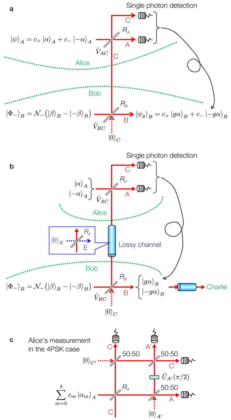
Figure 1: Scheme of quantum tele-amplification and quantum relay. a Tele-amplification of binary cat-state in an ideal lossless channel. $R_{A}$ and $R_{B}$ are the reflectivities of the BSs. b Loss tolerant quantum relay. $R_{E}$ is the reflectivity of the BS which models the lossy channel. c Alice’s four-port measurement for the case of 4PSK states.

The basic scheme of teleportation from Alice to Bob of a cat state qubit $\left|\psi\right\rangle_{A}=c_{+}\left|\alpha\right\rangle_{A}+c_{-}\left|-\alpha\right\rangle_{A}$, which is a variation of the schemes in refs. 20 and 21, is depicted in Fig. 1a. Bob prepares an odd cat state $\left|\Phi_{-}(\beta)\right\rangle_{B}={\cal{N_{-}}}\bigl{(}\left|\beta\right\rangle_{B}-\left|-\beta\right\rangle_{B}\bigr{)}$ with normalization $\cal{N_{-}}$ and splits it into an entangled cat state over paths B and C via a beam-splitter (BS) $\hat{V}_{BC}$ with reflectivity $R_{B}$. He sends one part of it to Alice at port C. She then combines it on an $R_{A}$-reflectivity BS with her input $\left|\psi\right\rangle_{A}$ at port A as

$$\left|\Psi\right\rangle_{ABC}=\hat{V}_{AC}\left|\psi\right\rangle_{A}\hat{V}_{BC}\left|\Phi\right\rangle_{B}\left|0\right\rangle_{C}.$$ (1)

She finally measures modes A and C by single-photon detectors. By conditioning port B on her measurement result, Bob can restore Alice’s input.

The amplitude of the resource cat state is set as $\beta=\alpha\sqrt{(1-R_{A})/R_{A}R_{B}},$ such that the components at port A turn into either the vacuum or a non-vacuum state. Then, when Alice’s detectors register a single photon at port A and nothing at port C – denoted (1,0) – Bob unambiguously obtains the state (see Appendix A)

$${}_{AC}\langle 1,0|\Psi\rangle_{ABC}\propto c_{+}\left|-g\alpha\right\rangle_{B}+c_{-}\left|g\alpha\right\rangle_{B},$$ (2)

where $g=\sqrt{(1-R_{A})(1-R_{B})/R_{A}R_{B}}$ is the gain parameter. By a simple $\pi$-phase shift, it can be transformed to Alice’s input $\left|\psi\right\rangle_{A}$, but with a modified amplitude $\alpha^{\prime}=g\alpha$. This process, previously suggested in ref. 3, we will call tele-amplification.

Unfortunately this tele-amplification is vulnerable to losses. Suppose the channel between Alice and Bob is subject to a linear loss $R_{E}$. The amplitude of the resource cat state should then be chosen as

$$\beta=\sqrt{\frac{1-R_{A}}{R_{A}R_{B}(1-R_{E})}}\alpha.$$ (3)

After conditioning on Alice’s detection event (1,0), Bob’s state gets entangled with an external mode E as

$$\left|\psi\right\rangle_{A}\left|0\right\rangle_{E}\mapsto c_{+}\left|-g\alpha\right\rangle_{B}\left|\varepsilon\right\rangle_{E}+c_{-}\left|g\alpha\right\rangle_{B}\left|-\varepsilon\right\rangle_{E}$$ (4)

with the modified gain including the loss rate $R_{E}$

$$g=\sqrt{\frac{(1-R_{A})(1-R_{B})}{R_{A}R_{B}(1-R_{E})}}.$$ (5)

Here $\varepsilon=\sqrt{(1-R_{A})R_{E}/R_{A}(1-R_{E})}\alpha$. Thus, the output at Bob is generally in a decohered state.

One can, however, see that if Alice’s inputs are restricted to classical components, $\left|\alpha\right\rangle$ or $\left|-\alpha\right\rangle$, as in Fig. 1b, the output state can be completely disentangled from the external mode. This means that the coherent states can be tele-amplified faithfully to the target states even through the lossy channel as

$$\left|\pm\alpha\right\rangle_{A}\mapsto\left|\pm g\alpha\right\rangle_{B}.$$ (6)

This is referred to as loss-tolerant quantum relay. In this context, Bob plays the role of an intermediate node, restores the target states $\left|\pm g\alpha\right\rangle_{B}$, and sends them to the terminal node, Charlie.

This simplest binary case can be extended into M-PSK coherent states. Let us show it for the 4-PSK case, $\left|\alpha_{m}\right\rangle,\,(\alpha_{m}=i^{m}\alpha,\,m=0,1,2,3)$. Bob should prepare a 4-component cat state

$$\left|\Phi\right\rangle_{B}={\cal N}\displaystyle\sum_{k=0}^{3}i^{k}\left|i^{k}\beta\right\rangle_{B}$$ (7)

as a resource. This state is beam-split, and is shared with Alice. We set $R_{A}=0.5$. As in Fig. 1c, Alice performs a four-port single-photon detection at paths A, A’, C, and C’ on this state. Depending on the set of results at the four ports, (A, A’, C, C’), the inputs are tele-amplified as

$$\begin{array}[]{llll}\left|\alpha_{m}\right\rangle&\mapsto&\left|g\alpha_{m}\right\rangle,&\mathrm{for}\,\,(0,1,1,1),\\ \left|\alpha_{m}\right\rangle&\mapsto&\left|ig\alpha_{m}\right\rangle,&\mathrm{for}\,\,(1,0,1,1),\\ \left|\alpha_{m}\right\rangle&\mapsto&\left|-g\alpha_{m}\right\rangle,&\mathrm{for}\,\,(1,1,0,1),\\ \left|\alpha_{m}\right\rangle&\mapsto&\left|-ig\alpha_{m}\right\rangle,&\mathrm{for}\,\,(1,1,1,0).\end{array}$$ (8)

Thus, the simple tele-amplification is performed for the result (0,1,1,1). Moreover the output state can be switched to another element by choosing an appropriate click pattern at Alice (see Appendix B).

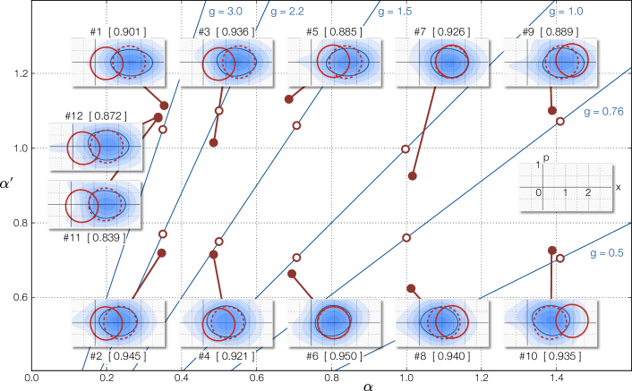
Figure 2: Measured results for the twelve cases. The blue straight lines represent $\alpha^{\prime}=g\alpha$. The open circles represent the sets of $\alpha$ and $g_{\mathrm{tg}}$ in Table I. The fidelities between the measured states and the targeted $\left|g_{\mathrm{tg}}\alpha\right\rangle$ are indicated by the numbers in brackets. Filled circles represent the amplitudes $\alpha$ ($\alpha^{\prime}$) of the coherent states that have the maximum fidelity with the measured input (output) states. Insets: Output state Wigner functions are shown in blue contour plots. The red solid and dashed circles are for the input and ideal targeted states, respectively.

The faithful relay itself can also be realized in a classical way, where Bob at the intermediate node performs an unambiguous state discrimination on the signal state, reproduces an amplified state for his confident result, and finally resends it to Charlie. The success probabilities of the two methods are compared in Appendix C. This classical relay cannot, however, be applied to a QKD relay node without the trusted node assumption. In contrast, a quantum relay can be carried out in the fully quantum domain, without Bob’s knowing the signal state itself, though at the expense of preparing the entangled cat state, and an appropriate entanglement verification session. Similar ideas for single-photon QKD were presented in refs. 22 and 23.

Our loss-tolerant quantum relay is particularly useful for extending the distance of QKD which uses PSK coherent states, such as B92 and BB84 ^{5; 6; 26}. Although the secure key generation probabilities at short distances slightly degrades from the original PSK-BB84, they can remain at reasonable levels up to much longer distances by the loss-tolerant quantum relay (see Appendix G).

We carried out an experimental demonstration of the tele-amplification in the simplest case of binary PSK as in Fig. 1b to realize Eq. (6). The resource cat state $\left|\Phi_{-}\right\rangle$ was generated by photon-subtraction from a squeezed vacuum with anti-squeezing along the real axis in phase space (Methods). Bob’s BS was set to $R_{B}=0.1$. For a given desired gain $g$, we varied $R_{A}$ according to Eq. (5). The resource cat-state amplitude $\beta$, experimentally tuned by the squeezing level, was then set by Eq. (3). The detector at port C was omitted with negligible effect on the outcomes since the events (A,C)=(1,1) would be rare. Bob’s output state was characterized by homodyne tomography.

We tested twelve settings as summarized in Table I. The five different input amplitudes $\alpha$ were real and ranged between 0.35 and 1.4. The protocol was carried out only for $\left|\alpha\right\rangle$ because the outcome for $\left|-\alpha\right\rangle$ would be trivially identical. The measured results are shown in Fig. 2. The blue straight lines are gain curves $\alpha^{\prime}=g\alpha$ in the $(\alpha,\alpha^{\prime})$ diagram. The open circles plotted along these lines represent sets of $\alpha$ and $g_{\mathrm{tg}}$ in Table I. The Wigner functions of the tomographically reconstructed tele-amplified output states $\hat{\rho}_{\mathrm{out}}$ are shown as blue contour plots in the insets. One contour level is highlighted for comparison with the targeted states $\left|g_{\mathrm{tg}}\alpha\right\rangle$ (red dashed) and the actual input states $\hat{\rho}_{\mathrm{in}}\approx\left|\alpha\right\rangle\!\left\langle\alpha\right|$ (red solid, also characterized by homodyne tomography). The discrepancies between $\hat{\rho}_{\mathrm{out}}$ and $\left|g_{\mathrm{tg}}\alpha\right\rangle$ are due to imperfections, including the deviation of the photon-subtracted state from the ideal resource cat, losses, impurity, and Alice’s use of an on/off detector instead of two single-photon detectors (see Appendix C). For each setting, we calculate which coherent states $\left|\alpha\right\rangle,\left|\alpha^{\prime}\right\rangle$ have the highest fidelity with the measured input and output states, respectively, that is, $\alpha=\mathrm{argmax}_{\gamma}\langle\gamma|\hat{\rho}_{\mathrm{in}}|\gamma\rangle$ and $\alpha^{\prime}=\mathrm{argmax}_{\gamma^{\prime}}\langle\gamma^{\prime}|\hat{\rho}_{\mathrm{out}}|\gamma^{\prime}\rangle$. These $(\alpha,\alpha^{\prime})$ pairs are marked as filled circles.

Despite the imperfections, the tele-amplification succeeded with high fidelities $\mathcal{F}=\langle g_{\mathrm{tg}}\alpha|\hat{\rho}_{\mathrm{out}}|g_{\mathrm{tg}}\alpha\rangle$ between 0.89 and 0.95 as shown next to each inset. The obtained amplitudes (filled circles) are close to the targeted ones (open circles) in almost all cases. The success probabilities were in the range 0.3% to 0.65% (Methods). For larger $\alpha^{\prime}$, the Wigner function shapes are slightly elongated due to the larger squeezing needed to produce those states. We note that our experimental settings were not fully optimized by taking into account spectral mode mismatch between the resource cat and input coherent states as well as between the APD and homodyne detectors. Had we done it, we estimate the achieved fidelities to have been 0.94–0.99.

The settings #11 and 12 had an additional 80% loss ($R_{E}=0.8$) in the channel from Bob to Alice. In #11, $R_{A}=0.5$ for the original lossless setting (as in #1), while in #12, $R_{A}=0.83$ as optimized according to Eq. (5), resulting in success probabilities of 0.17% and 0.11%. The fidelities with the target state are as high as 0.839 and 0.872, respectively, as compared with 0.901 in the lossless case. This demonstrates the loss tolerance of the protocol.

#	$\alpha$	$g_{\mathrm{tg}}$	$\beta$	$R_{A}$	$R_{E}$	$\mathcal{F}$
1	0.35	3.0	1.11	0.50	0	0.901
2	0.35	2.2	0.81	0.65	0	0.945
3	0.50	2.2	1.16	0.65	0	0.936
4	0.50	1.5	0.79	0.80	0	0.921
5	0.71	1.5	1.12	0.80	0	0.885
6	0.71	1.0	0.75	0.90	0	0.950
7	1.00	1.0	1.05	0.90	0	0.926
8	1.00	0.76	0.80	0.94	0	0.940
9	1.41	0.76	1.13	0.94	0	0.889
10	1.41	0.50	0.74	0.97	0	0.935
11	0.35	3.0	1.11	0.50	0.8	0.839
12	0.35	3.0	1.11	0.83	0.8	0.872

Table 1: Desired tele-amplification for the twelve settings of input coherent states and gains. $g_{\mathrm{tg}}$ is the targeted gain. The last column shows the obtained teleportation fidelities.

Teleportation of a cat-state qubit as in Eqs. (1- 13) is a prerequisite for CSQC. Interestingly, the tele-amplification allows to convert between different amplitude qubit bases. Although we previously generated such arbitrary cat qubits ^{18; 27}, it was not feasible to tele-amplify them with the current setup since three simultaneous APD clicks would be needed. Instead we simulated this protocol by accurately modelling the current experiment including all relevant practical imperfections (see Appendix F). Figure 3 shows the average fidelities between the teleported state for an input cat-state qubit and an output state from the model (Methods). For a wide range of input amplitudes $\alpha$ and output amplitudes $\alpha^{\prime}$, it is possible to surpass the classical limit of 2/3.

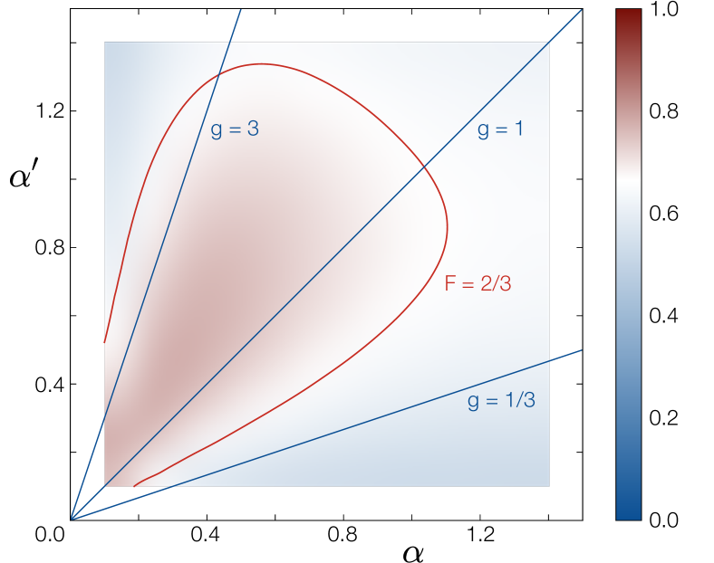
Figure 3: Simulated average qubit teleportation fidelity as a function of input ($\alpha$) and output state ($\alpha^{\prime}$) amplitudes. All relevant practical imperfections in our experimental setup, as described in Appendix F, are taken into account. The red curve labelled “F = 2/3” indicates the classical teleportation bound.

Finally we make a brief comparison between our scheme and the quantum noiseless amplifier with single-photon ancilla ^{28; 29; 30}. The latter is intended to noiselessly amplify a coherent state with an unknown amplitude at the cost of the success probability. In contrast, our scheme assumes the known amplitude $\alpha$ but instead enables one to tele-amplify PSK coherent states over a lossy channel with perfect fidelity and high success probability. It can also implement, in principle, the teleportation of their arbitrary superpositions.

In summary, we presented tele-amplification and loss-tolerant quantum relay of coherent states as the first operational application of optical cat states. The scheme is an essential building block for CSQC as well as quantum communications.

Methods

Experiment We generated the squeezed vacua at 860 nm wavelength from an OPO (optical parametric oscillator) continuously pumped with pump parameters between 0.15 and 0.31, corresponding to $\beta$ values of 0.78 to 1.15. We tapped off 5% of the squeezed beam on a BS and guided it to an APD. A click of the APD heralded the subtraction of a photon from the main beam ^{15; 27}. The state thus generated is a close approximation to the odd cat state $\left|\Phi_{-}\right\rangle$, and has been shown to provide near-perfect teleportation performance ³¹.

Whenever Alice’s APD clicked simultaneously with the heralding signal of the single-photon subtraction for the resource cat-state generation, the tele-amplification was successful, and we recorded a trace of the homodyne signal of Bob’s output state. The success probability is given by the ratio of the simultaneous click rate ($\sim$3–28 $s^{-1}$) to the photon subtraction click rate ($\sim$1000–4500 $s^{-1}$). It is mainly limited by detector and spectral filtering efficiency. To build the homodyne tomogram, we repeated this procedure 6000–24000 times for each fixed input state, with the local oscillator of the homodyne detector locked at phases $-180^{\circ},-150^{\circ},\ldots,150^{\circ}$ with respect to the input state. Note that the protocol succeeds as a single shot for an unknown input state – the repeated measurements with identical inputs are only needed for characterizing the process by homodyne tomography.

Alice’s input states were independently characterized by homodyne tomography at port C by setting $R_{A}=1$. To determine the input states accurately just at Alice’s BS, we correct their reconstruction for the detection efficiency and the propagation losses from that point to the homodyne detector. This total efficiency amounts to 88%. Likewise, in the reconstruction of Bob’s output states we correct for the overall detection efficiency of 94% but not for any propagation losses.

A more detailed description of the experimental setup and the state characterization can be found in Appendix E.

Simulation of cat-state qubit teleportation A cat-state qubit can be represented on a Bloch sphere as

$$\left|\psi(\alpha,\theta,\phi)\right\rangle = c_{+}\left|\mathrm{\alpha}\right\rangle+c_{-}\left|\mathrm{-\alpha}\right\rangle$$

$$= \mathrm{cos}\frac{\theta}{2}\left|\Phi_{+}(\alpha)\right\rangle+e^{i\phi}\mathrm{sin}\frac{\theta}{2}\left|\Phi_{-}(\alpha)\right\rangle,$$

where $|\Phi_{\pm}(\alpha)\rangle={\cal{N}}_{\pm}(\left|\alpha\right\rangle\pm\left|-\alpha\right\rangle)$ are the even/odd cat states with ${\cal{N}}_{\pm}=1/\sqrt{2(1\pm e^{-2\alpha^{2}})}$ and $c_{\pm}={\cal{N}}_{+}\mathrm{cos}\frac{\theta}{2}\pm{\cal{N}}_{-}e^{i\phi}\mathrm{sin}\frac{\theta}{2}.$

Given an input state $\left|\psi(\alpha,\theta,\phi)\right\rangle$, our model of the experiment, described in Appendix F, returns a teleported output state $\hat{\rho}_{\alpha,\theta,\phi}$. To quantify the performance of the qubit teleportation for specific settings of $\alpha$ and $\alpha^{\prime}=g_{\mathrm{tg}}\alpha$, we calculate the average fidelity of the teleported state with the target state by integrating over the Bloch sphere:

$$\mathcal{F}^{\mathrm{avg}}_{\alpha\rightarrow\alpha^{\prime}}=\int d\phi d\theta\frac{\sin\theta}{4\pi}\left\langle\psi(\alpha^{\prime},\theta,\phi)\right|\hat{\rho}_{\alpha,\theta,\phi}\left|\psi(\alpha^{\prime},\theta,\phi)\right\rangle.$$

The results for a range of amplitude settings are plotted in Fig. 3.

Acknowledgments

We acknowledge helpful discussions with K. Wakui, M. Takeoka, K. Hayasaka, M. Fujiwara, T. C. Ralph, A. P. Lund, K. Tamaki, and M. Koashi. This work was partly supported by the Quantum Information Processing Project in the Program for World-Leading Innovation Research and Development on Science and Technology (FIRST) and by a National Research Foundation of Korea (NRF) grant funded by the Korean Government (Ministry of Education, Science, and Technology) (No. 2010-0018295).

Author contributions

M.S. and J.S.N-N. formulated the basic protocol of tele-amplification and loss-tolerant quantum relay, inspired by a teleportation scheme by C.-W.L. and H.J.. J.S.N-N. and Y.E. carried out the experiment. J.S.N-N., C.-W.L., M.S. and H.J. performed the theoretical calculations. J.S.N-N. and M.S. wrote the paper with discussions and input from all the authors.

Appendix A Tele-amplification of a binary component cat-state

We first describe the tele-amplification of a binary component cat-state $\left|\psi(\alpha)\right\rangle_{A}=c_{0}\left|\alpha\right\rangle_{A}+c_{1}\left|-\alpha\right\rangle_{A}$ through a lossless channel. The whole three-mode state after the beam-splitting operation in Fig. 1a is given by

$$\left|\Psi\right\rangle_{ABC} = \hat{V}_{AC}\left|\psi(\alpha)\right\rangle_{A}\hat{V}_{BC}\left|\Phi\right\rangle_{B}\left|0\right\rangle_{C}$$ (9)

$$= {\cal{N}}c_{0}\left|\sqrt{1-R_{A}}\alpha-\sqrt{R_{A}R_{B}}\beta\right\rangle_{A}\left|\sqrt{1-R_{B}}\beta\right\rangle_{B}\left|-\sqrt{R_{A}}\alpha-\sqrt{(1-R_{A})R_{B}}\beta\right\rangle_{C}$$

$$- {\cal{N}}c_{0}\left|\sqrt{1-R_{A}}\alpha+\sqrt{R_{A}R_{B}}\beta\right\rangle_{A}\left|-\sqrt{1-R_{B}}\beta\right\rangle_{B}\left|-\sqrt{R_{A}}\alpha+\sqrt{(1-R_{A})R_{B}}\beta\right\rangle_{C}$$

$$+ {\cal{N}}c_{1}\left|-\sqrt{1-R_{A}}\alpha-\sqrt{R_{A}R_{B}}\beta\right\rangle_{A}\left|\sqrt{1-R_{B}}\beta\right\rangle_{B}\left|\sqrt{R_{A}}\alpha-\sqrt{(1-R_{A})R_{B}}\beta\right\rangle_{C}$$

$$- {\cal{N}}c_{1}\left|-\sqrt{1-R_{A}}\alpha+\sqrt{R_{A}R_{B}}\beta\right\rangle_{A}\left|-\sqrt{1-R_{B}}\beta\right\rangle_{B}\left|\sqrt{R_{A}}\alpha+\sqrt{(1-R_{A})R_{B}}\beta\right\rangle_{C}$$

where ${\cal{N}}=1/\sqrt{2[1-\exp(-2|\beta|^{2})]}$ is the normalization of the resource cat state $\left|\Phi\right\rangle_{B}$. We now impose a condition on the amplitude of the resource cat state

$$\beta=\sqrt{\frac{1-R_{A}}{R_{A}R_{B}}}\alpha$$ (10)

such that the components at port A turn into either of the vacuum or non-vacuum states as

$$\left|\Psi\right\rangle_{ABC} = {\cal{N}}c_{0}\left|0\right\rangle_{A}\left|g\alpha\right\rangle_{B}\left|-\frac{1}{\sqrt{R_{A}}}\alpha\right\rangle_{C}$$ (11)

$$- {\cal{N}}c_{0}\left|2\sqrt{1-R_{A}}\alpha\right\rangle_{A}\left|-g\alpha\right\rangle_{B}\left|\frac{1-2R_{A}}{\sqrt{R_{A}}}\alpha\right\rangle_{C}$$

$$+ {\cal{N}}c_{1}\left|-2\sqrt{1-R_{A}}\alpha\right\rangle_{A}\left|g\alpha\right\rangle_{B}\left|-\frac{1-2R_{A}}{\sqrt{R_{A}}}\alpha\right\rangle_{C}$$

$$- {\cal{N}}c_{1}\left|0\right\rangle_{A}\left|-g\alpha\right\rangle_{B}\left|\frac{1}{\sqrt{R_{A}}}\alpha\right\rangle_{C}$$

with the gain

$$g=\sqrt{(1-R_{A})(1-R_{B})/R_{A}R_{B}}.$$ (12)

Alice then performs single photon detection on paths A and C as shown in Fig. 1a, and selects single photon at port A and nothing at port C – denoted (1,0). Then Bob can unambiguously exclude the first and fourth terms in Eq. (11), and has the state

$${}_{AC}\langle 1,0|\Psi\rangle_{ABC}\propto\left|\psi(-g\alpha)\right\rangle_{B}.$$ (13)

In the case where the channel between Alice and Bob is subject to a linear loss with the rate $R_{E}$, one can consider an external mode E. Bob chooses the cat-state amplitude as

$$\beta=\sqrt{\frac{1-R_{A}}{R_{A}R_{B}(1-R_{E})}}\alpha.$$ (14)

The whole state before Alice’s measurement is

$$\left|\Psi\right\rangle_{ABCE}$$

$$=\hat{V}_{AC}\left|\psi\right\rangle_{A}\hat{V}_{EC}\hat{V}_{BC}\left|\Phi\right\rangle_{B}\left|0\right\rangle_{C}\left|0\right\rangle_{E}$$

$$={\cal{N}}c_{0}\left|0\right\rangle_{A}\left|g\alpha\right\rangle_{B}\left|-\frac{1}{\sqrt{R_{A}}}\alpha\right\rangle_{C}\left|-\varepsilon\right\rangle_{E}$$

$$-{\cal{N}}c_{0}\left|2\sqrt{1-R_{A}}\alpha\right\rangle_{A}\left|-g\alpha\right\rangle_{B}\left|\frac{1-2R_{A}}{\sqrt{R_{A}}}\alpha\right\rangle_{C}\left|\varepsilon\right\rangle_{E}$$

$$+{\cal{N}}c_{1}\left|-2\sqrt{1-R_{A}}\alpha\right\rangle_{A}\left|g\alpha\right\rangle_{B}\left|-\frac{1-2R_{A}}{\sqrt{R_{A}}}\alpha\right\rangle_{C}\left|-\varepsilon\right\rangle_{E}$$

$$-{\cal{N}}c_{1}\left|0\right\rangle_{A}\left|-g\alpha\right\rangle_{B}\left|\frac{1}{\sqrt{R_{A}}}\alpha\right\rangle_{C}\left|\varepsilon\right\rangle_{E}$$ (15)

with the gain

$$g=\sqrt{\frac{(1-R_{A})(1-R_{B})}{R_{A}R_{B}(1-R_{E})}}$$ (16)

and $\varepsilon=\sqrt{(1-R_{A})R_{E}/R_{A}(1-R_{E})}\alpha$.

Appendix B Extension to multi-ary coherent states

The binary case can be extended to $M$-ary phase-shift-keyed coherent states $\left|\alpha_{m}\right\rangle$, where

$$\alpha_{m}=\alpha u^{m},\quad u=e^{2\pi i/M}.$$ (17)

Here $\alpha_{0}=\alpha$ is taken to be real. The states are generated as

$$\left|\alpha_{m}\right\rangle=\hat{V}^{m}\left|\alpha_{0}\right\rangle$$ (18)

by modulating the phase of the coherent state $\left|\alpha\right\rangle$ with

$$\hat{V}=\exp\left(\frac{2\pi i}{M}\hat{n}\right).$$ (19)

An input state at Alice is generally a superposition state

$$\left|\psi\right\rangle_{A}=\sum_{m=0}^{M-1}c_{m}\left|\alpha_{m}\right\rangle_{A}.$$ (20)

Bob prepares a cat state for the entanglement resource,

$$\left|\Phi\right\rangle_{B}=\sum_{k=0}^{M-1}b_{m}\left|\beta_{m}\right\rangle_{B}$$ (21)

where $\beta_{m}=\beta u^{m}$ with $\beta$ real. In order to analyze the scheme and its performmance, we introduce the orthonormal basis $\{\left|\omega_{m}\right\rangle\}$ in the space spanned by $\{\left|\beta_{m}\right\rangle\}$ as follows

$$\left|\omega_{m}\right\rangle=\frac{1}{\sqrt{M\lambda_{m}}}\sum_{k=0}^{M-1}u^{-mk}\left|\beta_{k}\right\rangle$$ (22)

where

$$\lambda_{m}=\sum_{k=0}^{M-1}u^{-km}\left\langle\beta_{0}|\beta_{k}\right\rangle.$$ (23)

The orthonormality $\left\langle\omega_{m^{\prime}}|\omega_{m}\right\rangle=\delta_{m^{\prime},m}$ can be verified by a relation

$$\sum_{k=0}^{M-1}u^{(m-n)k}=M\delta_{m,n+lM}\,\,\,(\forall\text{ integer }l)$$ (24)

and that the Gram matrix $[\left\langle\beta_{k^{\prime}}|\beta_{k}\right\rangle]$ is cyclic. The coherent states can be expanded as

$$\left|\beta_{m}\right\rangle=\frac{1}{\sqrt{M}}\sum_{k=0}^{M-1}\sqrt{\lambda_{k}}u^{mk}\left|\omega_{k}\right\rangle.$$ (25)

Then one can see that

$$\hat{\rho}=\sum_{m=0}^{M-1}\left|\beta_{m}\right\rangle\left\langle\beta_{m}\right|=\sum_{m=0}^{M-1}\lambda_{m}\left|\omega_{m}\right\rangle\left\langle\omega_{m}\right|.$$ (26)

Thus $\lambda_{m}$ are the eigenvalues of the density operator of the ensemble $\{\left|\beta_{m}\right\rangle\}$. The mean photon number of the basis states is

$$\left\langle\omega_{m}\right|\hat{n}\left|\omega_{m}\right\rangle=\frac{\lambda_{m-1}}{\lambda_{m}}|\beta|^{2}.$$ (27)

To maximize the success probability of Alice’s measurement, one should use the $\left|\omega_{m}\right\rangle$ which has the maximum photon number for the entanglement resource. For relatively smaller $|\beta|$, it is the $\left|\omega_{M-1}\right\rangle$. In fact, the basis states can be represented by the number states as

$$\left|\omega_{m}\right\rangle=\sqrt{\frac{M}{\lambda_{m}}}e^{-\beta^{2}/2}\sum_{l=0}^{\infty}\frac{\beta^{m+lM}}{\sqrt{(m+lM)!}}\left|m+lM\right\rangle.$$ (28)

Thus $\left|\omega_{m}\right\rangle$ consists of a set of the photon number states $\{\left|m+lM\right\rangle;l=0,1,...\}$.

Now let us see the case of $M=4$ $(u=i)$. The basis states are explicitly given by

$$\left|\omega_{0}\right\rangle = \frac{2e^{-\beta^{2}/2}}{\sqrt{\lambda_{0}}}\Bigl{(}\left|0\right\rangle+\frac{\beta^{4}}{\sqrt{4!}}\left|4\right\rangle+\cdots\Bigr{)}$$

$$\left|\omega_{1}\right\rangle = \frac{2e^{-\beta^{2}/2}}{\sqrt{\lambda_{1}}}\Bigl{(}\beta\left|1\right\rangle+\frac{\beta^{5}}{\sqrt{5!}}\left|5\right\rangle+\cdots\Bigr{)}$$

$$\left|\omega_{2}\right\rangle = \frac{2e^{-\beta^{2}/2}}{\sqrt{\lambda_{2}}}\Bigl{(}\frac{\beta^{2}}{\sqrt{2!}}\left|2\right\rangle+\frac{\beta^{6}}{\sqrt{6!}}\left|6\right\rangle+\cdots\Bigr{)}$$

$$\left|\omega_{3}\right\rangle = \frac{2e^{-\beta^{2}/2}}{\sqrt{\lambda_{3}}}\Bigl{(}\frac{\beta^{3}}{\sqrt{3!}}\left|3\right\rangle+\frac{\beta^{7}}{\sqrt{7!}}\left|7\right\rangle+\cdots\Bigr{)}$$ (29)

with the eigenvalues

$$\begin{array}[]{lll}\lambda_{0}&=&2e^{-\beta^{2}}(\cosh\beta^{2}+\cos\beta^{2}),\\ \lambda_{1}&=&2e^{-\beta^{2}}(\sinh\beta^{2}+\sin\beta^{2}),\\ \lambda_{2}&=&2e^{-\beta^{2}}(\cosh\beta^{2}-\cos\beta^{2}),\\ \lambda_{3}&=&2e^{-\beta^{2}}(\sinh\beta^{2}-\sin\beta^{2}).\end{array}$$ (30)

The cat state for the entanglement resource is chosen as

$$\left|\Phi\right\rangle_{B}=\left|\omega_{3}\right\rangle_{B}=\frac{1}{\sqrt{4\lambda_{3}}}\sum_{k=0}^{M-1}u^{k}\left|\beta_{k}\right\rangle_{B}.$$ (31)

The above state is beam-split into paths B and C, the component of mode C is sent to Alice through a lossy channel, and then combined with the input at path A.

Bob chooses the cat-state amplitude as Eq. (14). The whole state before the measurement is given by

$$\left|\Psi\right\rangle_{BACE} = \sum_{m=0}^{3}c_{m}\sum_{k=0}^{3}\frac{u^{k}}{\sqrt{4\lambda_{3}}}\left|g\alpha u^{k}\right\rangle_{B}$$ (32)

$$\otimes \left|\sqrt{1-R_{A}}\alpha(u^{m}-u^{k})\right\rangle_{A}$$

$$\otimes \left|-\frac{\alpha}{\sqrt{R_{A}}}\Bigl{[}R_{A}u^{m}+(1-R_{A})u^{k}\Bigr{]}\right\rangle_{C}$$

$$\otimes \left|\varepsilon u^{k}\right\rangle_{E}$$

with the gain given by Eq. (16).

We set $R_{A}=0.5$. Alice further introduces additional modes A’ and C’ to implement the four-port single photon detection as shown in Fig. 1b. The state before the detection is given by

$$\left|\Psi\right\rangle_{BAA^{\prime}CC^{\prime}E} = \sum_{m=0}^{3}c_{m}\sum_{k=0}^{3}u^{k}\left|g\alpha u^{k}\right\rangle_{B}$$ (33)

$$\otimes \left|\alpha\frac{u^{m}-u^{k}}{2}\right\rangle_{A}$$

$$\otimes \left|-\alpha\frac{u^{m}+u^{k}}{2}\right\rangle_{C}$$

$$\otimes \left|\alpha\frac{u^{m}-u^{m+1}+u^{k}+u^{k+1}}{2\sqrt{2}}\right\rangle_{A^{\prime}}$$

$$\otimes \left|\alpha\frac{u^{m}+u^{m+1}+u^{k}-u^{k+1}}{2\sqrt{2}}\right\rangle_{C^{\prime}}$$

$$\otimes \left|\frac{R_{E}}{\sqrt{1-R_{E}}}\alpha u^{k}\right\rangle_{E}$$

When the loss can be neglected ($R_{E}=0$), the input $\left|\psi\right\rangle$ of Eq. (20) can be faithfully tele-amplified to the target state

$$\left|g\psi\right\rangle_{B}=\sum_{m=0}^{M-1}c_{m}\left|g\alpha_{m}\right\rangle_{B},$$ (34)

by selecting a set of Alice’s measurement result as (A, A’, C, C’)=(0,1,1,1), namely no count at port A while single-photon counts at port A’, C, and C’.

In the lossy case, it is impossible to teleport a superposition state faithfully. However, when an input is restricted to a classical state drawn from the set $\left|\alpha_{m}\right\rangle$, then the tele-amplification to the target pure state is possible. Actually depending on a set of the results at the four ports, (A, A’, C, C’), the inputs are tele-amplified as

$$\begin{array}[]{llll}\left|\alpha_{m}\right\rangle&\mapsto&\left|g\alpha_{m}\right\rangle,&\mathrm{for}\,\,(0,1,1,1),\\ \left|\alpha_{m}\right\rangle&\mapsto&\left|ig\alpha_{m}\right\rangle,&\mathrm{for}\,\,(1,0,1,1),\\ \left|\alpha_{m}\right\rangle&\mapsto&\left|-g\alpha_{m}\right\rangle,&\mathrm{for}\,\,(1,1,0,1),\\ \left|\alpha_{m}\right\rangle&\mapsto&\left|-ig\alpha_{m}\right\rangle,&\mathrm{for}\,\,(1,1,1,0).\end{array}$$ (35)

Appendix C On/off detection at Alice

In our experiment, Alice’s measurement is implemented by avalanche photodiodes (APDs) instead of ideal “single-photon detectors” that discriminate between “0”, “1” and “2 or more” photons. APDs cannot, however, discriminate photon numbers, but distinguish merely the vacuum or non-vacuum state, i.e. “off” or “on”. They are represented by the operators $\hat{\Pi}_{\mathrm{off}}=\left|0\right\rangle\left\langle 0\right|$ and $\hat{\Pi}_{\mathrm{on}}=\hat{I}-\left|0\right\rangle\left\langle 0\right|$. Then the tele-amplification described in the previous section should be corrected slightly. For example, Eq. (13) for the binary case becomes

$${}_{ABC}\langle\Psi|\hat{\Pi}_{\mathrm{on}}^{A}\hat{\Pi}_{\mathrm{off}}^{C}|\Psi\rangle_{ABC}=|\psi(-g\alpha)\rangle_{B}\langle\psi(-g\alpha)|\\ +\tanh\Bigl{(}\frac{\tilde{\alpha}}{2}\Bigr{)}|\tilde{\psi}(-g\alpha)\rangle_{B}\langle\tilde{\psi}(-g\alpha)|$$ (36)

where $|\tilde{\psi}(-g\alpha)\rangle=c_{0}\left|\alpha\right\rangle-c_{1}\left|-\alpha\right\rangle$ and $\tilde{\alpha}=2\sqrt{1-R_{A}}\alpha$. The second term is the correction. When $\alpha$ is small, the coefficient of the second term is small as $\tanh(\tilde{\alpha}/2)\sim\tilde{\alpha}/2$. In this regime, the tele-amplification would approximately work with on/off detection. However, in general, the second term cannot be ignored.

If the input state was a coherent state, i.e., $c_{0}=0$ or $c_{1}=0$, the above state would become a pure coherent state with the gain $g$, and on/off detection would be sufficient.

Appendix D Success probability

D.1 Loss tolerant quantum relay

In the binary case, the input is either of $\left|\alpha\right\rangle$ and $\left|-\alpha\right\rangle$. The whole state before Alice’s measurement is

$$\begin{split}\left|\Psi_{\pm}\right\rangle&=\hat{V}_{AC}\left|\pm\alpha\right\rangle_{A}\hat{V}_{EC}\hat{V}_{BC}\left|\Phi\right\rangle_{B}\left|0\right\rangle_{C}\left|0\right\rangle_{E}\\ &=\pm{\cal{N}}\left|0\right\rangle_{A}\left|\pm g\alpha\right\rangle_{B}\left|\mp\frac{1}{\sqrt{R_{A}}}\alpha\right\rangle_{C}\left|\mp\varepsilon\right\rangle_{E}\\ \mp{\cal{N}}&\left|\pm 2\sqrt{1-R_{A}}\alpha\right\rangle_{A}\left|\mp g\alpha\right\rangle_{B}\left|\pm\frac{1-2R_{A}}{\sqrt{R_{A}}}\alpha\right\rangle_{C}\left|\pm\varepsilon\right\rangle_{E}\end{split}$$ (37)

The success probability of the tele-amplification $\left|\pm\alpha\right\rangle_{A}\mapsto\left|\pm g\alpha\right\rangle_{B}$ is given by the expectation value of $\hat{\Pi}_{10}\equiv\hat{\Pi}_{\mathrm{on}}^{A}\otimes\hat{\Pi}_{\mathrm{off}}^{C}$ as

$$P_{\mathrm{Tele-amp}}^{(2)} = \frac{1}{2}\left\langle\Psi_{+}\right|\hat{\Pi}_{10}\left|\Psi_{+}\right\rangle+\frac{1}{2}\left\langle\Psi_{-}\right|\hat{\Pi}_{10}\left|\Psi_{-}\right\rangle$$ (38)

$$= \frac{\exp\left[-\frac{(1-2R_{A})^{2}}{R_{A}}\alpha^{2}\right]-\exp\left[-\frac{\alpha^{2}}{R_{A}}\right]}{2\left(1-\exp\left[-\frac{2(1-R_{A})}{R_{A}R_{B}(1-R_{E})}\alpha^{2}\right]\right)}.$$

In the case of 4-PSK states, the state before Alice’s measurement is given by

$$\left|\Psi_{m}\right\rangle = \sum_{k=0}^{3}u^{k}\left|g\alpha u^{k}\right\rangle_{B}$$ (39)

$$\otimes \left|\alpha\frac{u^{m}-u^{k}}{2}\right\rangle_{A}\left|-\alpha\frac{u^{m}+u^{k}}{2}\right\rangle_{C}$$

$$\otimes \left|\alpha\frac{u^{m}-u^{m+1}+u^{k}+u^{k+1}}{2\sqrt{2}}\right\rangle_{A^{\prime}}$$

$$\otimes \left|\alpha\frac{u^{m}+u^{m+1}+u^{k}-u^{k+1}}{2\sqrt{2}}\right\rangle_{C^{\prime}}$$

$$\otimes \left|\frac{R_{E}}{\sqrt{1-R_{E}}}\alpha u^{k}\right\rangle_{E}$$

The success probability of $\left|\alpha_{m}\right\rangle_{A}\mapsto\left|g\alpha_{m}\right\rangle_{B}$ is given by the expectation value of

$$\hat{\Pi}_{0111}\equiv\hat{\Pi}_{\mathrm{off}}^{A}\otimes\hat{\Pi}_{\mathrm{on}}^{A^{\prime}}\otimes\hat{\Pi}_{\mathrm{on}}^{C}\otimes\hat{\Pi}_{\mathrm{on}}^{C^{\prime}}$$ (40)

as

$$P_{\mathrm{Tele-amp}}^{(4)} = \frac{1}{4}\sum_{k=0}^{3}\left\langle\Psi_{m}\right|\hat{\Pi}_{0111}\left|\Psi_{m}\right\rangle$$ (41)

$$= \left\langle\Psi_{0}\right|\hat{\Pi}_{0111}\left|\Psi_{0}\right\rangle$$

$$= \frac{(1-e^{-\alpha^{2}/2})^{2}(1-e^{-\alpha^{2}})}{4\lambda_{3}(\frac{\alpha^{2}}{R_{B}(1-R_{E})})}$$

where

$$\lambda_{3}(x)=2e^{-x}(\sinh x-\sin x).$$ (42)

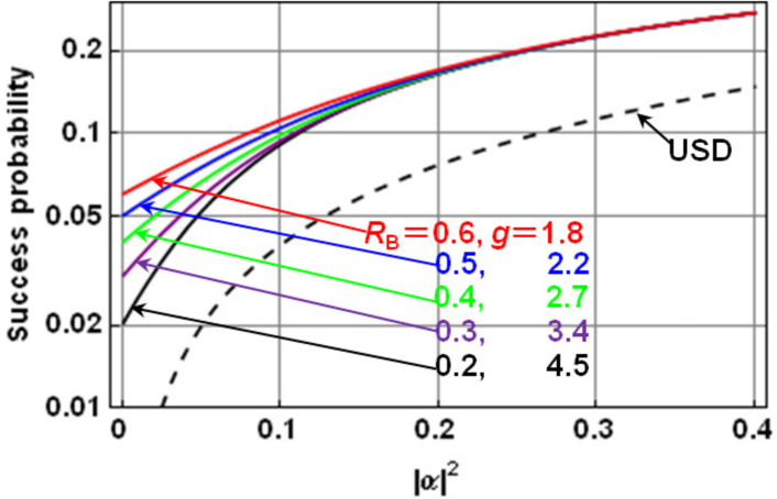
Figure 4: Success probabilities for the case of the BPSK coherent states. The channel loss is assumed be 80% ($R_{E}=0.8$). The solid lines are for the quantum relay with several cases of the amplification gains, while the dashed line is for the measure-resend strategy with the unambiguous state discrimination.

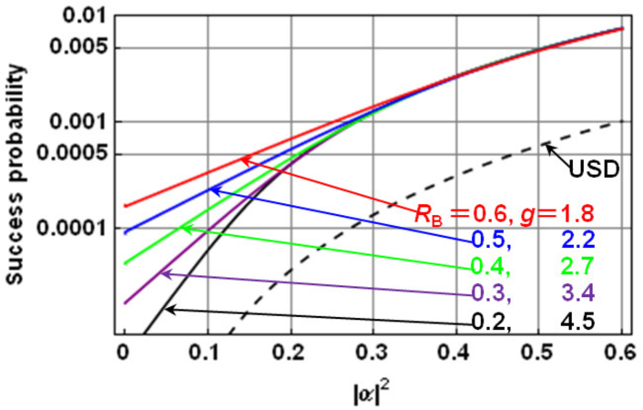
Figure 5: Success probabilities for the case of the 4PSK coherent states. The channel loss is assumed be 80% ($R_{E}=0.8$).

D.2 Measure-resend strategy

The task to relay attenuated coherent states to the receiver, converting them faithfully to the target amplified states, can also be realized by a classical strategy. A typical one is a measure-resend strategy. In the intermediate node, Bob has attenuated states $\{\left|\sqrt{1-R_{E}}\alpha_{m}\right\rangle\}$. He tries to discriminate them unambiguosly without errors, but at a finite success rate, referred to as unambiguous state discrimination (USD), and then prepare a target amplified state $\left|g\sqrt{1-R_{E}}\alpha_{m}\right\rangle$ for the measurement result $m$. The success rate is well known for this kind of equally probable symmetric states ¹. Denoting $\left|\gamma_{m}\right\rangle=\left|\sqrt{1-R_{E}}\alpha_{m}\right\rangle$ and using the eigenvalues and the diagonalizing vectors of the density operator

$$\hat{\rho}=\sum_{m=0}^{M-1}\left|\gamma_{m}\right\rangle\left\langle\gamma_{m}\right|=\sum_{m=0}^{M-1}\lambda_{m}\left|\omega_{m}\right\rangle\left\langle\omega_{m}\right|,$$ (43)

the success rate is given by

$$P_{\mathrm{USD}}=\min_{k}{\lambda_{k}}.$$ (44)

The signal states are represented as

$$\left|\gamma_{m}\right\rangle = \left|\sqrt{1-R_{E}}\alpha_{m}\right\rangle$$ (45)

$$= \frac{1}{\sqrt{M}}\sum_{k=0}^{M-1}\sqrt{\lambda_{k}}u^{mk}\left|\omega_{k}\right\rangle.$$

The detection operators are given by

$$\hat{\Pi}_{m}=\frac{\Lambda}{M}P_{USD}\left|\gamma_{m}^{\bot}\right\rangle\left\langle\gamma_{m}^{\bot}\right|$$ (46)

for the signal state $\left|\gamma_{m}\right\rangle$, using the reciprocal states

$$\left|\gamma_{m}^{\bot}\right\rangle=\frac{1}{\sqrt{\Lambda}}\sum_{k=0}^{M-1}\frac{u^{mk}}{\sqrt{\lambda_{k}}}\left|\omega_{k}\right\rangle$$ (47)

where $\Lambda=\sum_{k}\lambda_{k}^{-1}$. They satisfy the orthogonality relation

$$\left\langle\gamma_{m}^{\bot}|\gamma_{m^{\prime}}\right\rangle=\sqrt{\frac{M}{\Lambda}}\delta_{m,m^{\prime}}.$$ (48)

The operator for the inconclusive result is given by

$$\hat{\Pi}_{F}=\hat{I}-\sum_{m=0}^{M-1}\hat{\Pi}_{m}.$$ (49)

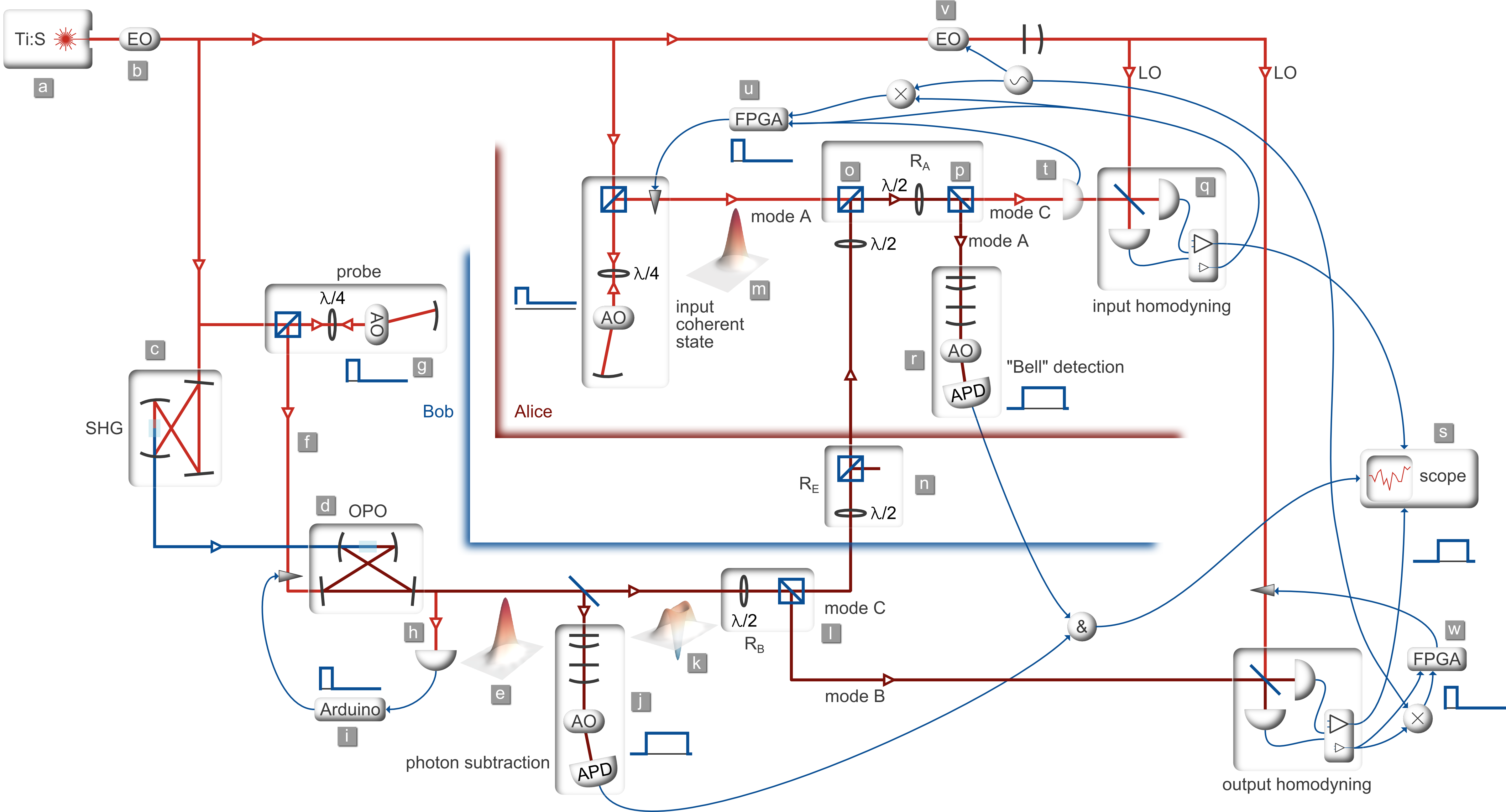
Figure 6: Sketch of the experimental setup for tele-amplification of a coherent state from Alice to Bob using shared entanglement in the form of a photon-subtracted squeezed vacuum state.

D.3 Numerical results

Numerical results of the success probabilities in the case of $R_{E}=0.8$ (80% loss) are shown in Fig. 4 for the BPSK coherent states, and in Fig. 5 for the 4PSK coherent states, in comparison with that by the measure-resend strategy. The quantum relay can attain higher success rates than that by the above measure-resend strategy. In the case of 4PSK states, the difference is as high as ten times.

Appendix E Experimental details

E.1 Setup

The most relevant elements of the experimental setup are sketched in Fig. 6 and described in the following.

Resource state generation

The output of an 860 nm continuous-wave Ti:Sapph laser (a) is phase-modulated by an EOM (b) for Pound-Drever locking of the SHG and OPO cavities. Parts of the beam are tapped off for use as local oscillators, coherent input beam, probe beam and cavity locking beams, but the main part is frequency-doubled in the second harmonic generator (c). The 430 nm output of this SHG pumps a bow-tie configuration optical parametric oscillator (OPO, d) with a PPKTP crystal and a HWHM bandwidth of $\gamma/2\pi=4.5\ \mathrm{MHz}$. The down-converted light leaving the cavity is in a squeezed vacuum state (e). A probe beam (f) is injected into the OPO for the purpose of locking phases and filtering cavities further downstream.

The whole experiment is running in an alternating lock/measure cycle at a rate of 10 kHz. The probe beam is thus switched on and off by double-passes through two acousto-optical modulators (only one shown in the figure) that are driven for only 20% of the 10 kHz cycle time, as indicated by the little blue pulse diagram (g) (this diagram is repeated for other relevant parts of the setup).

In order to act as a phase-reference for the squeezing, the probe beam is locked in phase with the squeezed quadrature by observing its classical parametric amplification in the OPO through a $<$1% tap-off of the OPO output (h). To obtain an error-signal, the probe’s phase is dithered on a piezo-mounted mirror by a micro-controller unit (Arduino) which also processes the detected signal and provides feedback to lock the phase (i).

A photon is subtracted from the squeezed vacuum at random times by the detection on an avalanche photo-diode (APD) detector, placed after a 5% tapping beam-splitter and two frequency-filtering cavities (j). The APD is protected from the strong probe beam by an AOM that directs the OPO output to the APD only during the intervals when the probe beam is switched off. The resulting photon-subtracted squeezed vacuum (PSSV) state (k) is the resource of entanglement in our protocol, after it is split into two modes propagating towards the Alice and Bob sections of the setup. In the description of the protocol in the main section, a fraction $R_{B}=0.1$ is reflected towards Alice. In the actual experiment (and in the setup sketch), Alice’s fraction $R_{B}$ is actually taken as the transmitted part of a variable beam-splitter fixed at 90% reflection (l). Bob’s share of the entangled state is directed towards a homodyne detector for output state analysis.

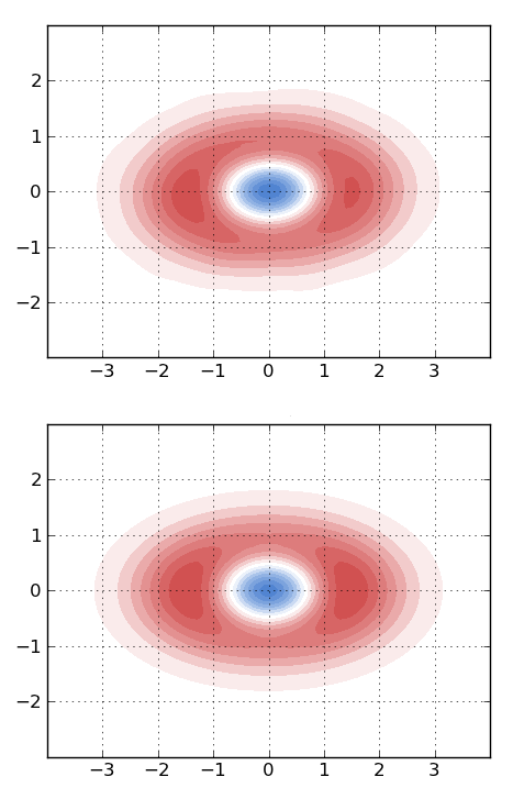
Figure 7: Wigner function for one of the PSSV states used as approximations for the odd cat resource state, in this case with $\epsilon=0.20$. The upper is experimentally generated and tomographically reconstructed, while the lower one is obtained from our model. The fidelity between them is above 98%, showing the validity of the model.

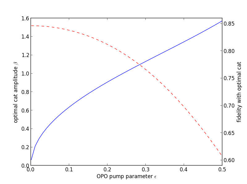
Figure 8: Relation between OPO pump parameter $\epsilon$ for the production of realistic PSSV states and the amplitude of the cat state $\left|\Phi_{-}(\beta)\right\rangle$ that maximizes the mutual fidelity. The blue curve indicates these optimal $\beta$ amplitudes, while the dashed red curve shows the corresponding fidelities. In the experiment, we used $\epsilon$ in the range 0.15–0.31.

The amount of squeezing produced by the OPO determines the amplitude of the cat-like PSSV state. It is regulated by the pump parameter $\epsilon=\sqrt{P_{\mathrm{pump}}/P_{\mathrm{threshold}}}$. To find what cat amplitude $\beta$ a given pump parameter corresponds to, we model the PSSV as in Ref. [23] of the main text. Here, we include the OPO temporal correlations, the temporal modes of the APD and homodyne detection (described in the following section), the 96% escape efficiency of the OPO, the 95% propagation efficiency towards the beam-splitter (l), the 5% tapping ratio, the $\sim$10% overall APD detection efficiency, and the filtering bandwidth to find a $\hat{\rho}_{\mathrm{PSSV}}$ that closely emulates the actually produced states. Fig. 7 shows an example of an experimentally generated PSSV state and, for comparison, the modelled state with equivalent parameters. We then maximize for $\beta$ the state’s fidelity with a true cat state, $\left\langle\Phi_{-}(\beta)\right|\hat{\rho}_{\mathrm{PSSV}}\left|\Phi_{-}(\beta)\right\rangle$, and get the $\epsilon\rightarrow\beta$ correspondence plotted in Fig. 8 and thereby the $\beta$ values of Table 1 in the main text.

Input state and teleportation

Alice’s input coherent state (m) is prepared in a configuration of two double-pass AOMs similar to that used for the OPO probe beam, with a strong phase locking beam switched on during the 20% locking part of the 10 kHz cycle. However, instead of switching the light completely off during the remaining 80% of the cycle, a weak amplitude beam is generated instead. This is done by switching to a lower voltage RF driving signal for the AOM.

The share of the entangled PSSV state propagating from Bob to Alice in mode C is optionally subjected to a loss at a variable beam-splitter (n) before it is overlapped with her input state on a polarizing beam splitter (PBS) in orthogonal polarizations (o). A half-waveplate followed by another PBS (p) then interferes the two modes as the protocol’s $R_{A}$ reflectivity beam-splitter. When characterizing the input state, $R_{A}$ is set to 1, which means that all of the input state is sent towards the homodyne detector (q). Otherwise, when running the tele-amplification protocol, $R_{A}$ is set to its appropriate value, and the output of the beamsplitter in mode A is sent towards an APD (r) with the same frequency filtering and chopping configuration as that in (j).

The detection events from the two APDs are correlated with digital timing electronics that pick out simultaneous events and triggers the acquisition of Bob’s homodyne signal at a fast digital oscilloscope (s). The detected photo-currents are subsequently temporally filtered on a PC to extract the measured quadrature values, as described in the following section.

Phase locking

For the tele-amplification protocol to work, the input states $\left|\pm\alpha\right\rangle$ should be interfered in-phase with the anti-squeezed quadrature of the entangled PSSV state. We do this by putting a normal intensity detector (t) at the mode C output port of the beamsplitter instead of Alice’s homodyne detector (q). The detected interference signal between the probe portions of the input coherent state beam and the PSSV state beam is used as the input to an FPGA-based lock unit, which provides feedback to the phase of the input beam (u). When the two beams are interfered at 90^∘, we get the desired phase relation, since the PSSV probe was locked to the squeezed quadrature.

The phase of the local oscillators (LO) in the two homodyne detectors can be locked to arbitrary phases relative to the PSSV probe by using a combination of DC and side-band detection of the interference between the LO and the probe beam. An 8 MHz phase modulation is applied to the LO (v), and the interference signals observed by the fast homodyne detectors (from a separate low-gain amplification output) are demodulated at that same frequency. This provides an interference signal that is 90^∘ out of phase with the DC signal. In the FPGA lock units (u,w), the two signals are added with weighting factors corresponding to the desired LO phase in phase space, resulting in an error signal for the feedback to piezo-mounted mirrors in the LO beam path (in the case of Bob’s output homodyner) or in the input beam path (for Alice).

All phase locks are engaged only during the intervals of the 10 kHz experiment cycle in which the probe beams are turned on. For the remaining time, the feedback signals are just held at their last actively set value.

E.2 Quantum state tomography

Temporal modes

The squeezed vacuum has a bandwidth given by the OPO’s HWHM of $\gamma/2\pi=4.5\ \mathrm{MHz}$. Conditioned on an APD click at time $t_{0}$, the continuous-wave squeezed vacuum is converted into a temporally localized PSSV state in a temporal mode around $t_{0}$ which, in the low-squeezing limit, has the form² $\exp(-\gamma|t-t_{0}|)$. The filter cavities in front of the APD, needed to remove the photons down-converted into the many non-degenerate OPO resonances, modify the temporal mode to be

$$f(t)\propto\gamma^{-1}e^{-\gamma|t-t_{0}|}-\kappa^{-1}e^{-\kappa|t-t_{0}|},$$ (50)

where $\kappa/2\pi\approx 25\ \mathrm{MHz}$ is the combined bandwidth of the two filters, approximated by a single Lorentzian spectral profile. This will also be the temporal mode of the teleported output state in the low-squeezing limit. For the state tomography, we therefore extract a single quadrature value from the continuous photo current signal of the homodyne detector by integrating it over a mode $f_{\mathrm{HD,out}}(t)$ equal to the one in Eq. (50). At higher squeezing levels, the optimal mode function is not that simple ³, but in this work we stick to the simple expression for all squeezing levels.

An interesting, but also complicating aspect of our current implementation of the tele-amplification protocol is that the input and output states are in rather different spectral modes: The input coherent state is derived directly from the narrow-band laser, whereas the entangled PSSV state is in the broadband mode described above. At a first glance it would appear like the two modes will not interfere well and the teleportation will fail. However, the spectral response of Alice’s APD is very broad, so it is unable to distinguish the modes. Thereby it can be said that the detection itself induces the interference between the input and the entangled state. Another way to see it is in the time domain: compared to the cw input beam and the $\sim 1/\gamma$ extent of the PSSV state, the temporal response of the APD ($\sim$350 ps jitter) is essentially delta function-like. Within this short time window, almost no phase shift will occur between the different frequency components, so interference will not be destroyed.

One problem we do get from this spectral mismatch, however, is the issue of which temporal mode, $f_{\mathrm{HD,in}}(t)$ to use for the definition of the coherent input state. As the beam is continuous, the choice of temporal mode can be done arbitrarily. The photon number $n_{\mathrm{in}}$ within the chosen mode will be proportional to the width of the mode function, so to obtain a desired coherent state the intensity of the beam should be adjusted inversely proportional to that width. In our experiment we make the rather natural choice to use the $f_{\mathrm{HD,out}}(t)$ mode, such that we observe the same temporal mode in both the input and the output homodyne tomography. The measured $\alpha$ and $\alpha^{\prime}$ values in Fig. 2 of the main paper are therefore directly comparable.

However, this mode is not the one detected by the APD. Since the APD with its delta function-like response is preceded by filtering cavities which act as delays for incoming fields, its temporal mode can be approximately described as a single-sided exponential decay, with time constant given by the filter bandwidth,

$$f_{\mathrm{APD}}(t)\propto e^{-\kappa|t-t_{0}|}H(t_{0}-t),$$ (51)

with $H(t)$ being the Heaviside step function. Because the PSSV entangled state is temporally localized, as opposed to the input state, the ratio of the photon numbers of the two states, $n_{\mathrm{in}}/n_{\mathrm{PSSV}}$ will be different within the different modes $f_{\mathrm{HD,in}}(t)$ and $f_{\mathrm{APD}}(t)$. There is therefore a mismatch between the input state amplitude, $\alpha$, that we expect to have and the amplitude actually seen by Alice’s APD, which is the one to induce the teleportation. Thus, the $\beta$ and $R_{A}$ values that we experimentally adjusted to match a given $\alpha$ were actually not optimal, and this resulted in output-to-target fidelities that were lower than we could have otherwise obtained. In a possible follow-up experiment, it would be advisable to consider this issue of the input state amplitude in more detail. Simulations indicate that with optimized settings, fidelities could have reached 0.94–0.99.

State reconstruction

For a given realization of the tele-amplification, we construct a homodyne tomogram of the output (and input) state by repeating the state preparation, on/off detection and conditional homodyne detection multiple times, with the LO phase of the homodyne detector fixed at various angles. After filtering the oscilloscope traces with the chosen temporal mode, as described above, the obtained quadrature values are normalized by vacuum traces recorded under the same experimental conditions while we also pay attention to proper offset correction of the traces, which can be particularly tricky for the measurement of the input coherent state. That gives us a homodyne tomogram like the one shown in Fig. 9. From this we reconstruct an estimate of the underlying quantum state using the maximum likelihood method ⁴. As mentioned in the Methods section, we correct for the non-perfect detector efficiencies in order to get the most accurate characterization of the protocol.

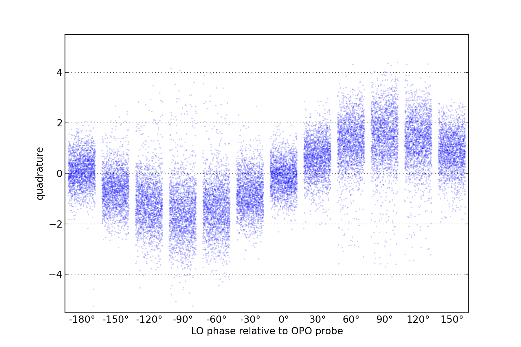
Figure 9: Example tomogram, showing the 12 $\times$ 2000 quadrature values of the homodyne measurement of the output state in tele-amplification #5.

The phase values in the figure indicate the relative phase between the local oscillator and the OPO-injected probe beam. The probe beam is locked to the squeezed quadrature of the PSSV state, and Alice’s input coherent beam is locked at 90^∘ to the probe beam. Since we define our phase space in such a way that the anti-squeezing is aligned along the $x$-axis and the input states have real amplitudes (i.e. also along the $x$-axis), the 90^∘ phase of the LO should correspond to the $x$-quadrature. We therefore rotate the reconstructed quantum state by $-90^{\circ}$ in phase space - the free choice of global phase.

Appendix F Modelling of qubit teleportation

To simulate the performance of our tele-amplifier setup in the case where the input is an arbitrary coherent state qubit

$$\left|\psi(\alpha,\theta,\phi)\right\rangle=\mathrm{cos}\frac{\theta}{2}\left|\Phi_{+}(\alpha)\right\rangle+e^{i\phi}\mathrm{sin}\frac{\theta}{2}\left|\Phi_{-}(\alpha)\right\rangle,$$ (52)

we set up a model for the protocol, using Wigner function formalism.

As the input state to be teleported, we took a pure qubit state of the above form. The initial resource state was a squeezed vacuum state with appropriate squeezing levels. In the experiment, the squeezed vacuum state within the homodyne-observed mode $f_{\mathrm{HD,out}}(t)$ is not pure. The impurity due to this mode selection can be modelled quite well by propagating the initially pure squeezed vacuum through a 92% transmission beam-splitter. The losses suffered by the photon-subtracted squeezed vacuum were similarly modelled by virtual beam-splitters, taking account of the 96% escape efficiency of the OPO, the 5% tapping ratio for the photon subtraction, and the 95% propagation efficiency towards the separating beam-splitter. Alice’s detector was modelled as an on/off detector with 10% efficiency, roughly corresponding to our APD’s detection efficiency and the transmission of the spectral filters.

For a given input amplitude $\alpha$ and desired output amplitude $\alpha^{\prime}$, we simulate the tele-amplification process for 168 evenly distributed qubit states on the $(\theta,\phi)$ Bloch sphere and calculate the fidelity between the output states and the targeted states $\left|\psi(\alpha^{\prime},\theta,\phi)\right\rangle$. This results in a “fidelity map” like the one in Fig. 10 for every $(\alpha,\alpha^{\prime})$ setting. It is clear that the teleportation works best for coherent state inputs (near 100% fidelity) and for states near the North Pole (which is the even cat) and not very well for states near the South Pole (odd cat). By averaging over the Bloch sphere, we obtain an average fidelity for the outcomes of the protocol for the given $(\alpha,\alpha^{\prime})$ pair, giving one value for the average fidelity plot in Fig. 3 of the main text.

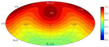
Figure 10: Bloch sphere map of the fidelities between modelled and targeted outcomes of the $\left|\psi(\alpha,\theta,\phi)\right\rangle\rightarrow\left|\psi(\alpha^{\prime},\theta,\phi)\right\rangle$ tele-amplification, in this case for $\alpha=0.4$ and $\alpha^{\prime}=0.6$. The averaged fidelity here is 77%.

Appendix G Application to quantum key distribution

The tele-amplification scheme would be useful to improve the performance of quantum key distribution (QKD) schemes which use phase-shifted coherent-state signals, such as B92 protocol with BPSK states ^{5; 6} and BB84 protocol with 4PSK states ⁷. The tele-amplifications of BPSK and 4PSK states could be applied to B92 and BB84, respectively. The B92 with BPSK states would be more interesting from the viewpoint of practical implementation because the necessary cat-state resources are readily available in laboratories. Unfortunately, however, its security proof and performace evaluation when the tele-amplification is included are more involved. In contrast, BB84 protocol with 4PSK states can be analyzed more clearly with the tele-amplification.

Therefore we consider the BB84 scheme where the key information is encoded in the relative phase of a coherent-state reference pulse and a coherent-state signal pulse as

$$\left|\tilde{0}_{X}\right\rangle = \left|\alpha\right\rangle_{R}\otimes\left|\alpha\right\rangle_{A}$$ (53a)

$$\left|\tilde{1}_{X}\right\rangle = \left|\alpha\right\rangle_{R}\otimes\left|-\alpha\right\rangle_{A}$$ (53b)

$$\left|\tilde{0}_{Y}\right\rangle = \left|\alpha\right\rangle_{R}\otimes\left|i\alpha\right\rangle_{A}$$ (53c)

$$\left|\tilde{1}_{Y}\right\rangle = \left|\alpha\right\rangle_{R}\otimes\left|-i\alpha\right\rangle_{A}$$ (53d)

where mode A is for the signal pulse while mode R for the reference pulse ⁷. This scheme is referred to as the 4PSK-BB84 with reference pulse. The amplitude $\alpha$ is understood as the one at the receiver Bob. It reduces from $\alpha_{\mathrm{in}}$ at Alice by the channel loss as

$$\alpha=\eta(L)\alpha_{\mathrm{in}}$$ (54)

where

$$\eta(L)=10^{-\xi L/10}$$ (55)

with the distance $L$ and the channel loss rate $\xi$. The phase of $\alpha$ is defined relative to a fixed classical phase reference frame that Eve can access. Alice emits one of the four states. Bob randomly chooses one of two measurement apparatuses, the X-basis or the Y-basis measurement, and measures the signal. In the X-basis measurement, the two modes are first combined on a balanced beam splitter as

$$\hat{V}\left|\alpha\right\rangle_{R}\left|\alpha\right\rangle_{A} = \left|\sqrt{2}\alpha\right\rangle_{R}\left|0\right\rangle_{A}$$ (56a)

$$\hat{V}\left|\alpha\right\rangle_{R}\left|-\alpha\right\rangle_{A} = \left|0\right\rangle_{R}\left|-\sqrt{2}\alpha\right\rangle_{A}$$ (56b)

then directed to two on/off detectors described by operators

$$\hat{\Pi}_{\mathrm{off}} = e^{-\nu}\sum^{\infty}_{m=0}(1-\eta_{B})^{m}\left|m\right\rangle\left\langle m\right|$$ (57a)

$$\hat{\Pi}_{\mathrm{on}} = \hat{I}-\hat{\Pi}_{\mathrm{off}}$$ (57b)

where $\nu$ is the dark count probability and $\eta_{B}$ is the detection efficiency. We define a POVM for making raw keys “0” and “1”, and an inconclusive outcome “2” by

$$\hat{\Pi}_{0}^{X} = \hat{V}^{\dagger}\left(\hat{\Pi}_{\mathrm{on}}^{R}\otimes\hat{\Pi}_{\mathrm{off}}^{A}+\frac{1}{2}\hat{\Pi}_{\mathrm{on}}^{R}\otimes\hat{\Pi}_{\mathrm{on}}^{A}\right)\hat{V}$$ (58a)

$$\hat{\Pi}_{1}^{X} = \hat{V}^{\dagger}\left(\hat{\Pi}_{\mathrm{off}}^{R}\otimes\hat{\Pi}_{\mathrm{on}}^{A}+\frac{1}{2}\hat{\Pi}_{\mathrm{on}}^{R}\otimes\hat{\Pi}_{\mathrm{on}}^{A}\right)\hat{V}$$ (58b)

$$\hat{\Pi}_{2}^{X} = \hat{V}^{\dagger}\hat{\Pi}_{\mathrm{off}}^{R}\otimes\hat{\Pi}_{\mathrm{off}}^{A}\hat{V}.$$ (58c)

We have three kinds of probabilities, $P_{\mathrm{c}}$ for correctly outputting the bit 0 (1) given the signal $\tilde{0}_{X}$ ($\tilde{1}_{X}$), $P_{\mathrm{e}}$ for incorrectly outputting the bit 0 (1) given the signal $\tilde{1}_{X}$ ($\tilde{0}_{X}$), and $P_{\mathrm{i}}$ for inconclusive outcome

$$P_{\mathrm{c}} = \left\langle\tilde{0}_{X}\right|\hat{\Pi}^{X}_{0}\left|\tilde{0}_{X}\right\rangle=\left\langle\tilde{1}_{X}\right|\hat{\Pi}^{X}_{1}\left|\tilde{1}_{X}\right\rangle$$ (59)

$$= \frac{1}{2}\left(1-e^{-\nu-2\eta_{B}|\alpha|^{2}}\right)(1+e^{-\nu})$$

$$P_{\mathrm{e}} = \left\langle\tilde{0}_{X}\right|\hat{\Pi}^{X}_{1}\left|\tilde{0}_{X}\right\rangle=\left\langle\tilde{1}_{X}\right|\hat{\Pi}^{X}_{0}\left|\tilde{1}_{X}\right\rangle$$ (60)

$$= \frac{1}{2}\left(1+e^{-\nu-2\eta_{B}|\alpha|^{2}}\right)(1-e^{-\nu})$$

$$P_{\mathrm{i}} = \left\langle\tilde{0}_{X}\right|\hat{\Pi}^{X}_{2}\left|\tilde{0}_{X}\right\rangle=\left\langle\tilde{1}_{X}\right|\hat{\Pi}^{X}_{2}\left|\tilde{1}_{X}\right\rangle$$ (61)

$$= e^{-2\nu-2\eta_{B}|\alpha|^{2}}.$$

Similarly, the Y-basis measurement is described by a POVM

$$\hat{\Pi}^{Y}_{0} = e^{i\frac{\pi}{2}\hat{n}_{A}}\hat{V}^{\dagger}\Bigl{(}\hat{\Pi}^{R}_{\mathrm{on}}\otimes\hat{\Pi}^{A}_{\mathrm{off}}$$ (62a)

$$+\frac{1}{2}\hat{\Pi}^{R}_{\mathrm{on}}\otimes\hat{\Pi}^{A}_{\mathrm{on}}\Bigr{)}\hat{V}e^{-i\frac{\pi}{2}{\hat{n}_{A}}}$$

$$\hat{\Pi}^{Y}_{1} = e^{i\frac{\pi}{2}\hat{n}_{A}}\hat{V}^{\dagger}\Bigl{(}\hat{\Pi}^{R}_{\mathrm{off}}\otimes\hat{\Pi}^{A}_{\mathrm{on}}$$ (62b)

$$+\frac{1}{2}\hat{\Pi}^{R}_{\mathrm{on}}\otimes\hat{\Pi}^{A}_{\mathrm{on}}\Bigr{)}\hat{V}e^{-i\frac{\pi}{2}{\hat{n}_{A}}}$$

$$\hat{\Pi}^{Y}_{2} = e^{i\frac{\pi}{2}\hat{n}_{A}}\hat{V}^{\dagger}\hat{\Pi}^{R}_{\mathrm{off}}\otimes\hat{\Pi}^{S}_{\mathrm{off}}\hat{V}e^{-i\frac{\pi}{2}{\hat{n}_{A}}}.$$ (62c)

where the factor $e^{i\frac{\pi}{2}{\hat{n}_{A}}}$ is for shifting the phase. Eliminating the inconclusive outcomes, the filtered fraction for sifted keys is defined by

$$Q=1-P_{\mathrm{i}}$$ (63)

and the bit error rate (BER) is defined by

$$\delta=\frac{P_{\mathrm{e}}}{Q}$$ (64)

Then the upper bound for the phase error rate (PER) is given by

$$\delta_{\mathrm{ph}} = \delta+4{\Delta^{\prime}}(1-{\Delta^{\prime}})(1-2\delta)$$ (65)

$$+ 4(1-2{\Delta^{\prime}})\sqrt{{\Delta^{\prime}}(1-{\Delta^{\prime}})\delta(1-\delta)}$$

where

$$\Delta^{\prime} = \frac{\Delta}{Q}$$ (66a)

$$\Delta = \frac{1}{2}\left[1-e^{-\alpha_{\mathrm{in}}^{2}}\left(\cos\alpha^{2}_{\mathrm{in}}+\sin\alpha^{2}_{\mathrm{in}}\right)\right].$$ (66b)

The quantity $\Delta$ specifies the imbalance of the “coin” for the choice of X and Y bases depending on the states overlap among $\{\left|\alpha_{\mathrm{in}}\right\rangle,\left|-\alpha_{\mathrm{in}}\right\rangle,\left|i\alpha_{\mathrm{in}}\right\rangle,\left|-i\alpha_{\mathrm{in}}\right\rangle\}$. The secure key generation probability is given by

$$G=\frac{1}{2}Q\left[1-H(\delta)-H(\delta_{\mathrm{ph}})\right]$$ (67)

where $H(x)$ is the binary Shannon entropy

$$H(x)=-x\log_{2}x-(1-x)\log_{2}(1-x).$$ (68)

Now let us consider an extention of this BB84 implementation to a tele-amplification assisted scheme. The signals sent by Alice are $\alpha_{m}^{\mathrm{in}}=\alpha_{\mathrm{in}}u^{m}$ where $u=i$ and $m=$0, 1, 2 and 3. The signals first arrive at the relay node, referred to as Amy, and are then relayed to the receiver at the terminal node, referred to as Bob. The total distance between Alice and Bob is $L$. The relay node Amy is located at the distance $xL$ from Alice, where $0<x<1$. The input coherent-state amplitude to the tele-amplifier at Amy is $\alpha_{m}=\sqrt{\eta(xL)}\alpha_{\mathrm{in}}u^{m}$. Bob prepares the resource cat state, beam-splits it, and sends Amy one half of the split cat-state over the distance $(1-x)L$. At the relay node, Amy combines it with the signal state $\left|\alpha_{m}\right\rangle_{A}$ on the beam splitter, and measures them by the four-port interferometric receiver. For simplicity, we assume that the single photons can be detected with perfect efficiency at the four ports. Three-photon coincidence counts at these ports herald the successful tele-amplification events. The dark count effect can be negligible by this multi-photon coincidence filtering. Bob finally receives the tele-apmplified signal $\left|g\alpha_{m}\right\rangle_{B}$, which is subject to the X or Y basis measurement. The gain is now a function of $x$ and $L$

$$g(x,L)=\sqrt{\frac{1-R_{B}}{R_{B}\eta[(1-x)L]}}.$$ (69)

Then the security proof in ref. 7 can be applied to the tele-amplification assisted BB84 provided that the reference pulse arrives at Bob so as to be in $\left|g(x,L)\sqrt{\eta(xL)}\alpha_{\mathrm{in}}\right\rangle_{R}\otimes\left|g(x,L)\sqrt{\eta(xL)}\alpha_{\mathrm{in}}u^{m}\right\rangle_{B}$. The filtering fraction $Q$, the BER $\delta$, the PER $\delta_{\mathrm{ph}}$ and $\Delta^{\prime}$ are given by replacing ${\alpha}$ in Eqs. (63), (64), (65), and (66) with the new one $g(x,L)\sqrt{\eta(xL)}\alpha_{\mathrm{in}}$. Here note that the signal attenuation occurs only for the channel interval between Alice and Amy over a distance $xL$. In the remaining channel with a distance $(1-x)L$, the signal attenuation is compensated by the cat-assisted amplification with the gain $g(x,L)$.

The secure key generation probability is finally given by multiplying the expression in Eq. (67) by the success probability of the tele-amplification as

$$G=\frac{1}{2}P_{\mathrm{Suc}}Q\left[1-H(\delta)-H(\delta_{\mathrm{ph}})\right].$$ (70)

Some numerical results are shown in Fig. 11 as a function of the transmission distance. In the following, the dark count probability is $\nu=10^{-6}$, and the detection efficiency of the receiver Bob is $\eta_{B}=0.2$. The dashed and dotted lines correspond to the 4PSK-BB84 with reference pulse. In this PSK coherent-state scheme, an eavesdropper Eve can effectively perform the photon-number splitting attack with phase information. So the input coherent-state amplitude should be set small. In Fig. 11, the dashed and dotted lines correspond to $|\alpha_{\mathrm{in}}|^{2}=0.008$ and 0.001, respectively. The key generation probabilities decrease more rapidly than that of the phase-randomized decoyed scheme. The solid lines represent the performances of the tele-amplification assisted BB84 with $R_{B}=0.2$. It can be seen that the secure key generation probabilities are smaller than those without tele-amplification at short distances, however, they can remain at reasonable levels up to longer distances. The input coherent-state amplitude $\alpha_{\mathrm{in}}$ is allowed to be larger in the tele-amplification assisted BB84. The red and brown lines are the cases where the relay node Amy is located closer to Bob, namely $x=0.8$ and $x=0.6$, respectively. The blue and black lines are the cases where Amy is located at $0.4L$ from Alice, with $|\alpha_{\mathrm{in}}|^{2}=0.2$ and 0.3, respectively. The green line is the case where Amy is located much closer to Alice, namely $x=0.2$ with $|\alpha_{\mathrm{in}}|^{2}=0.05$.

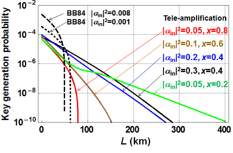
Figure 11: The secure key generation probabilities as a function of distance. The dashed and dotted lines correspond to BB84 without tele-amplification. The solid lines correspond to tele-amplification assisted BB84 where $R_{B}=0.2$. For all the cases, the dark count probability is $\nu=10^{-6}$, and the detection efficiency of the receiver Bob is $\eta_{B}=0.2$.

The performance of the green line is remarkable, however, one should prepare the resource cat-state with a much larger amplitude. The mean photon number of the resource cat state is given by

$$\beta(x,L)^{2}=\frac{\eta(xL)\alpha_{\mathrm{in}}^{2}}{\eta[(1-x)L]R_{B}}.$$ (71)

It is shown in Fig. 12. To extend the distance beyond 200 km, the resource cat-state should include more than a hundred photons.

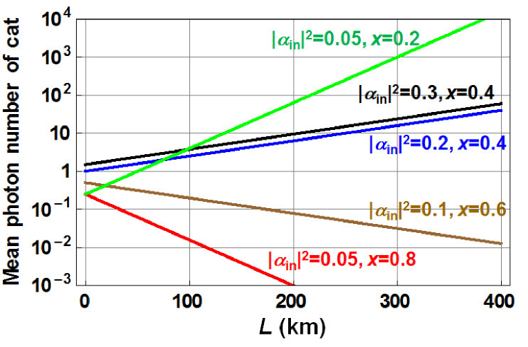
Figure 12: The mean photon numbers of the required cat states as a function of distance.

The essential effect brought by the tele-amplification is simply the improvement of the channel transmittance

$$\eta(L)\rightarrow g(x,L)^{2}\eta(xL)$$ (72)

but on the other hand also the reduction of the detection rate due to the additional filtering at the relay node. We plot the channel transmittance in Fig. 13. For $x<0.5$, the channel turns to be an amplifier as a whole. It is clearly seen in the BER and PER as shown in Figs. 14 and Fig. 15. They also decrease with the distance (black, blue and green lines). Actually there is no degradation of the signal-to-noise ratio as the distance increases. So the sudden fall of the key generation probability at a certain distance due to the dark count noise does not appear (see Fig. 11). For $x>0.5$, on the other hand, the BER and PER increase with the distance. In particular, the PER is the dominant error.

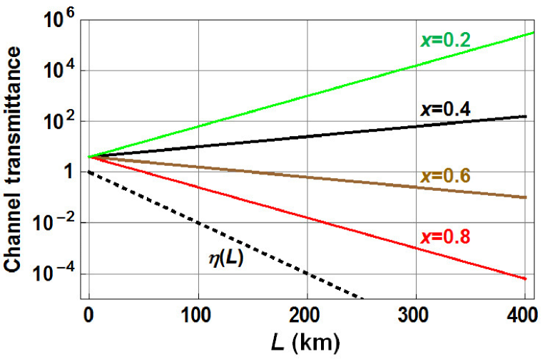
Figure 13: The channel transmittance as a function of distance. The dashed line corresponds to the original channel without the tele-amplificcation.

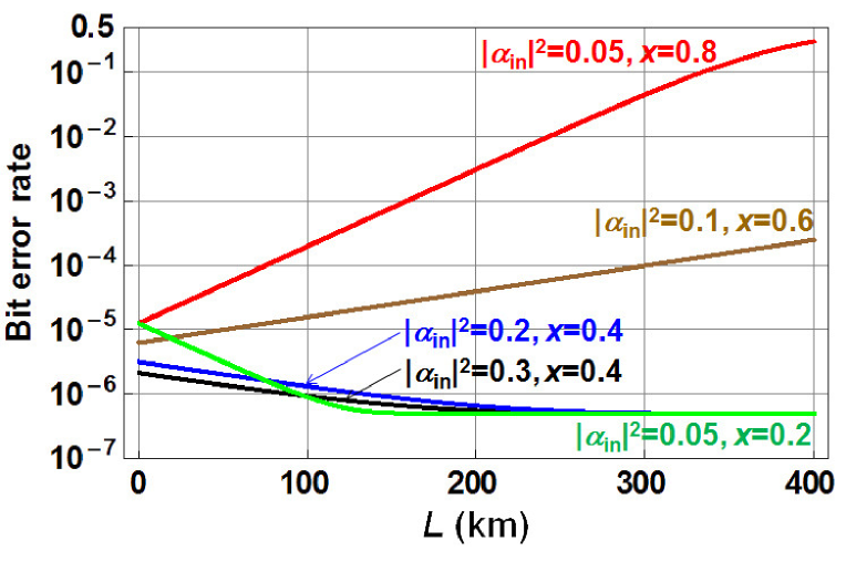
Figure 14: The BER as a function of distance.

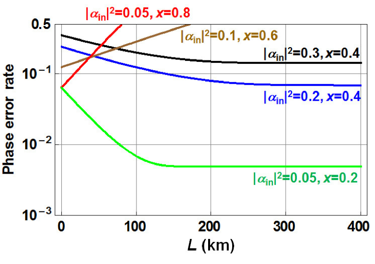
Figure 15: The PER as a function of distance.

The success rate of the tele-amplification decreases with the distance as shown in Fig. 16. This directly leads to the decrease of the key generation probability.

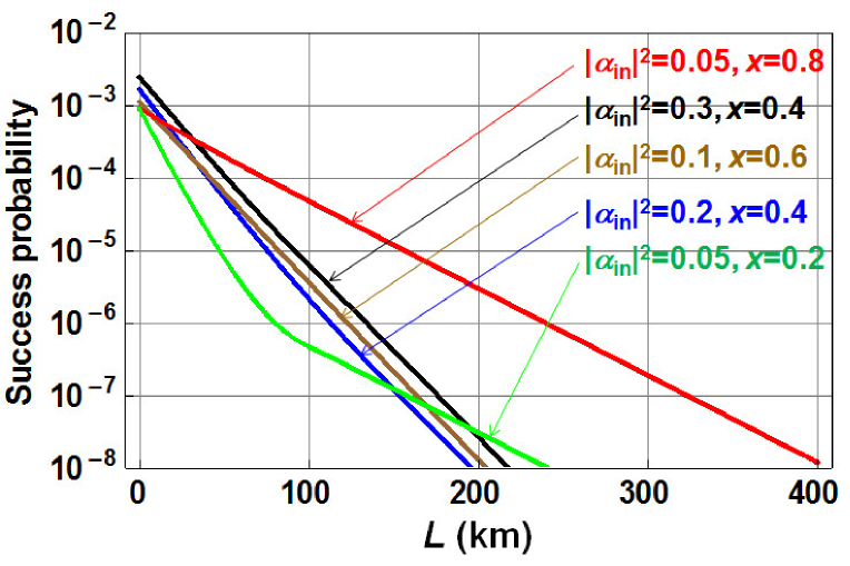
Figure 16: The success rate of the tele-amplification as a function of distance.

References

- (1) Cochrane, P. T., Milburn, G. J. & Munro, W. J. Macroscopically distinct quantum-superposition states as a bosonic code for amplitude damping. Phys. Rev. A 59, 2631–2634 (1999).
- (2) Jeong, H. & Kim, M. S. Efficient quantum computation using coherent states. Phys. Rev. A 65, 042305 (2002).
- (3) Ralph, T. C., Gilchrist, A., Milburn, G., Munro, W. J. & Glancy, S. Quantum computation with optical coherent states. Phys. Rev. A 68, 042319 (2003).
- (4) Jeong, H. & Ralph, T. C. Schrödinger cat states for quantum information processing. in Cerf, N. J., Leuchs G. & Polzik, E. S., eds., Quantum Information with Continuous Variables of Atoms and Light, Ch. 9 (Imperial College Press, 2007).
- (5) Lund, A. P., Ralph, T. C. & Haselgrove, H. L. Fault-tolerant linear optical quantum computing with small-amplitude coherent states. Phys. Rev. Lett. 100, 030503 (2008).
- (6) Gerry, C., Benmoussa, A. & Campos, R. Nonlinear interferometer as a resource for maximally entangled photonic states: Application to interferometry. Phys. Rev. A 66, 013804 (2002).
- (7) Joo, J., Munro, W. J. & Spiller, T. Quantum metrology with entangled coherent states. Phys. Rev. Lett. 107, 083601 (2011).
- (8) Sangouard, N. et al. Quantum repeaters with entangled coherent states. J. Opt. Soc. Am. B 27, A137–A145 (2010).
- (9) Brask, J. B. et al. Hybrid long-distance entanglement distribution protocol. Phys. Rev. Lett. 105, 160501 (2010).
- (10) Giovannetti, V. et al. Classical capacity of the lossy bosonic channel: The exact solution. Phys. Rev. Lett. 92, 027902 (2004).
- (11) Sasaki, M., Sasaki-Usuda, T., Izutsu, M. & Hirota, O. Realization of a collective decoding of code-word states. Phys. Rev. A 58, 159–164 (1998).
- (12) Waseda, A., Takeoka, M., Sasaki, M., Fujiwara, M. & Tanaka, H. Quantum detection of wavelength-division-multiplexing optical coherent signals. J. Opt. Soc. Am. B 27, 259–265 (2010).
- (13) Ourjoumtsev, A., Tualle-Brouri, R., Laurat, J. & Grangier, P. Generating optical Schrödinger kittens for quantum information processing. Science 312, 83–86 (2006).
- (14) Neergaard-Nielsen, J. S., Nielsen, B. M., Hettich, C., Mølmer, K. & Polzik, E. S. Generation of a superposition of odd photon number states for quantum information networks. Phys. Rev. Lett. 97, 083604 (2006).
- (15) Wakui, K., Takahashi, H., Furusawa, A. & Sasaki, M. Photon subtracted squeezed states generated with periodically poled KTiOPO4. Opt. Express 15, 3568–3574 (2007).
- (16) Ourjoumtsev, A., Jeong, H., Tualle-Brouri, R. & Grangier, P. Generation of optical ’Schrödinger cats’ from photon number states. Nature 448, 784–786 (2007).
- (17) Takahashi, H. et al. Generation of large-amplitude coherent-state superposition via ancilla-assisted photon subtraction. Phys. Rev. Lett. 101, 233605 (2008).
- (18) Neergaard-Nielsen, J. S. et al. Optical continuous-variable qubit. Phys. Rev. Lett. 105, 053602 (2010).
- (19) Lee, N. et al. Teleportation of nonclassical wave packets of light. Science 332, 330–333 (2011).
- (20) van Enk, S. J. & Hirota, O. Entangled coherent states: Teleportation and decoherence. Phys. Rev. A 64, 022313 (2001).
- (21) Jeong, H., Kim, M. & Lee, J. Quantum-information processing for a coherent superposition state via a mixed entangled coherent channel. Phys. Rev. A 64, 052308 (2001).
- (22) Jacobs, B., Pittman, T. & Franson, J. Quantum relays and noise suppression using linear optics. Phys. Rev. A 66, 052307 (2002).
- (23) Collins, D., Gisin, N. & De Riedmatten, H. Quantum relays for long distance quantum cryptography. J. Mod. Opt. 52, 735–753 (2005).
- (24) Koashi, M. Unconditional security of coherent-state quantum key distribution with a strong phase-reference pulse. Phys. Rev. Lett. 93, 120501 (2004).
- (25) Tamaki, K., Lütkenhaus, N., Koashi, M. & Batuwantudawe, J. Unconditional security of the Bennett 1992 quantum-key-distribution scheme with a strong reference pulse. Phys. Rev. A 80, 032302 (2009).
- (26) Lo, H.-K. & Preskill, J. Security of quantum key distribution using weak coherent states with nonrandom phases. Quant. Inf. Comp. 7, 431–458 (2007).
- (27) Takeoka, M. et al. Engineering of optical continuous-variable qubits via displaced photon subtraction: multimode analysis. J. Mod. Opt. 58, 266–275 (2011).
- (28) Xiang, G. Y., Ralph, T. C., Lund, A. P., Walk, N. & Pryde, G. J. Heralded noiseless linear amplification and distillation of entanglement. Nature Photon. 4, 316–319 (2010).
- (29) Zavatta, A., Fiurášek, J. & Bellini, M. A high-fidelity noiseless amplifier for quantum light states. Nature Photon. 5, 52–60 (2010).
- (30) Ferreyrol, F., Blandino, R., Barbieri, M., Tualle-Brouri, R. & Grangier, P. Experimental realization of a nondeterministic optical noiseless amplifier. Phys. Rev. A 83, 063801 (2011).
- (31) Brańczyk, A. & Ralph, T. C. Teleportation using squeezed single photons. Phys. Rev. A 78, 052304 (2008).

References

- (1) Chefles, A. and Barnett, S. M. Optimum unambiguous discrimination between linearly independent symmetric states. Phys. Lett. A 250, 223–229 (1998).
- (2) Mølmer, K. Non-Gaussian states from continuous-wave Gaussian light sources. Phys. Rev. A 73, 063804 (2006).
- (3) Nielsen, A. E. B. and Mølmer, K. Single-photon-state generation from a continuous-wave nondegenerate optical parametric oscillator. Phys. Rev. A 75, 023806 (2007).
- (4) Lvovsky, A. I. Iterative maximum-likelihood reconstruction in quantum homodyne tomography. J. Opt. B: Quantum Semiclass. Opt. 6, S556–S559 (2004).
- (5) Koashi, M. Unconditional security of coherent-state quantum key distribution with a strong phase-reference pulse. Phys. Rev. Lett. 93, 120501 (2004).
- (6) Tamaki, K., Lütkenhaus, N., Koashi, M. & Batuwantudawe, J. Unconditional security of the Bennett 1992 quantum-key-distribution scheme with a strong reference pulse. Phys. Rev. A 80, 032302 (2009).
- (7) Lo, H.-K. and Preskill, J. Security of quantum key distribution using weak coherent states with nonrandom phases. Quant. Inf. Comp. 7, 431–458 (2007).