Abstract

We study the case of a bright (L$>$L^⋆) barred spiral galaxy from the rich cluster A 3558 in the Shapley supercluster core ($z$=0.05) undergoing ram-pressure stripping. Integral-field spectroscopy with WiFeS at the 2.3m ANU, complemented by imaging in ultra violet (GALEX), $B$ and $R$ (ESO 2.2m WFI), H$\alpha$ (Magellan), $K$ (UKIRT), 24$\mu$m and 70$\mu$m (Spitzer), allows us to reveal the impact of ram pressure on the interstellar medium. With these data we study in detail the kinematics and the physical conditions of the ionized gas and the properties of the stellar populations. We observe one-sided extraplanar ionized gas along the full extent of the galaxy disc, extending $\sim$13 kpc in projection from it. Narrow-band H$\alpha$ imaging resolves this outflow into a complex of knots and filaments, similar to those seen in other cluster galaxies undergoing ram-pressure stripping. The gas velocity field is complex with the extraplanar gas showing signature of rotation, while the stellar velocity field is regular and the $K$-band image shows a symmetric stellar distribution. We use line-ratio diagnostics to ascertain the origin of the observed emission. In all parts of the galaxy, we find a significant contribution from shock excitation, as well as emission powered by star formation. Shock-ionized gas is associated with the turbulent gas outflow and highly attenuated by dust (A_v=1.5-2.3 mag). All these findings cover the whole phenomenology of early-stage ram-pressure stripping. Intense, highly obscured star formation is taking place in the nucleus, probably related to the bar, and in a region 12 kpc South-West from the centre. These two regions account for half of the total star formation in the galaxy, which overall amounts to 7.2$\pm$2.2 M_⊙yr^-1. In the SW region we identify a starburst characterized by a $\sim 5\times$ increase in the star-formation rate over the last $\sim$100 Myr, possibly related to the compression of the interstellar gas by the ram pressure. The scenario suggested by the observations is supported and refined by ad hoc N-body/hydrodynamical simulations which identify a rather narrow temporal range for the onset of ram-pressure stripping around t$\sim$60 Myr ago, and an angle between the galaxy rotation axis and the intra-cluster medium wind of $\sim 45^{\circ}$. The ram pressure is therefore acting at an intermediate angle between face-on and edge-on. Taking into account that the galaxy is found $\sim$1 Mpc from the cluster centre in a relatively low-density region, this study shows that ram-pressure stripping still acts efficiently on massive galaxies well outside the cluster cores, as also recently observed in the Virgo cluster.

Keywords: galaxies: evolution – galaxies: ISM – galaxies: intergalactic medium – galaxies: clusters: general – galaxies: stellar content – galaxies: clusters: individual: A3558

1 Introduction

Both the current properties and the past evolution of galaxies are strongly dependent on their environment (e.g. Blanton et al. 2005) and mass (e.g. Baldry et al. 2006, Haines et al. 2007). The environment is a determinant for both the morphology-density (Dressler, 1980; Dressler et al., 1997) and the star formation-density (Butcher & Oemler, 1984; Lewis et al., 2002; Kauffmann et al., 2004) relations: late-type, blue, star-forming galaxies are predominant in the field, while early-type, red, passive galaxies are preferentially found in galaxy clusters. This suggests that blue galaxies accreted from the field have been transformed into the passive S0s and dEs found in local clusters. A key question in galaxy evolution is therefore, how does the harsh cluster environment act to transform the spiral galaxies accreted from the field into passive S0s and dEs?

Several mechanisms dependent upon the environment have been proposed and investigated in detail and all of them serve to kinematically disturb spiral galaxies and/or deplete their reservoirs of gas, and so quench star formation. These physical processes include gravitational and tidal interactions amongst galaxies (Toomre & Toomre, 1972; Moore et al., 1996), between galaxies and the cluster gravitational field (Byrd & Valtonen 1990), galaxy mergers (Barnes & Hernquist, 1991), group-cluster collisions (Bekki, 2001), ram-pressure (Gunn & Gott, 1972) and viscous stripping (Nulsen, 1982), evaporation (Cowie & Songalia, 1977) and ‘starvation’ (Larson et al., 1980).

Since these mechanisms are characterized by different time-scales and efficiencies which depend, in turn, on the properties of both the galaxies and their environment, they can differentially affect the galaxy properties (Boselli & Gavazzi 2006; Haines et al. 2007). Over the last ten years, the development of huge spectroscopic surveys such as the Sloan Digital Sky Survey (SDSS), plus the availability of panoramic far ultra-violet – far infra-red (FUV–FIR) data from the GALEX and Spitzer space telescopes have allowed the impact of environment on star formation to be quantified in unprecedented detail. However, because they only consider the global properties of each galaxy (e.g. stellar mass, star-formation rate), they are unable to identify which process(es) are behind these transformations, except indirectly by statistical comparison of trends with predictions from cosmological simulations (e.g. Balogh et al., 2000; Haines et al., 2009). What is fundamentally required are direct “smoking-gun” observations of galaxies in the process of being transformed via interaction with their environment. The physical processes behind this transformation can then be distinguished by resolving their impacts on the gas contents, kinematics and star formation of the galaxies.

Ram pressure resulting from the passage of the galaxy through the hot and dense intra-cluster medium (ICM) can effectively remove the cold gas supply (Gunn & Gott, 1972; Abadi et al., 1999) and thus rapidly terminate ongoing star formation in cluster galaxies. This process could explain the lower star formation rates (SFRs; e.g. Balogh et al. 2000) and the redder colours (Bamford et al., 2009) seen in cluster galaxies with respect to the field population. Nevertheless, ram-pressure stripping, as originally proposed by Gunn & Gott (1972) requires, in principle, the presence of a dense ICM. Thus, its evolutionary effect would be limited to cluster cores where the gas discs of massive spirals are rapidly truncated.

In the last decade ram-pressure stripping (RPS) has been extensively studied using hydrodynamical simulations (e.g. Roediger & Hensler 2005; Roedigger & Brugger 2006; Kronberger at al. 2008a; Kapferer et al. 2009b; Tonnesen & Bryan 2009; Bekki 2009; Jáchym et al. 2009) describing the RPS process as function of galaxy parameters (stellar mass, inclination, orbit, velocity, mass of the gas halo, structure of the interstellar medium, etc.) and the density and structure of the ICM, suggesting a number of observables which can be used as diagnostics of its occurrence, intensity, and stage. With a 3–D hydrodynamical simulation, Marcolini et al. (2003) found that RPS may extend to poorer environments for low-mass galaxies which, thanks to their lower escape velocities, are easier to strip. RPS also directly affects the density and temperature structure of hot halo gas of galaxies and is relevant in the starvation mechanism in clusters and groups (Larson et al., 1980; Bekki et al., 2002; McCarthy et al., 2008).

The characteristic signatures of RPS are the presence of gas outflows, distortion and ultimate truncation of the gaseous disc without corresponding distortion of the old stellar component (e.g. Kenney et al 2004; 2008; 2011). Such features have been observed in numerous cluster spirals (e.g. Vogt et al. 2004; Chung et al. 2009). Ram pressure can also compress and shock the interstellar medium (ISM) enhancing the star formation in the inner disc (Byrd & Valtonen, 1990; Fujita & Nagashina, 1999). Tails of stripped gas may also be present, whose nature and evolution depend also on the properties of the ISM (Roediger & Brüggen, 2008; Tonnesen & Bryan, 2010).

Considering both the theoretical predictions and the observable effects, it follows that the detection of the stripped gas is a key step in order to better understand the role of RPS, but also of tidal stripping, in the transformation of galaxies from their actively star-forming phase to their passive phase. The stripped gas in cluster galaxies has been detected through narrow-band H$\alpha$ imaging (e.g. Gavazzi et al. 2001; Yagi et al. 2007, 2010; Yoshida et al. 2002; Kenney et al. 2008, Smith et al. 2010), through HI imaging (e.g. Oosterloo & van Gorkom 2005; Chung et al. 2007; Haynes et al. 2007; Koopmann et al. 2008), in X–ray images (e.g. Irwin & Sarazin 1996; Wang et al. 2004; Sun & Vikhlinin 2005; Sun et al. 2006; 2010; Machacek et al. 2006; Kim et al. 2008) and with multi-band observations (e.g. Crowl et al. 2005; Cortese et al. 2007; Abramson et al. 2011).

The presence of gas outside of the galaxy disc could also arise from mechanisms other than RPS, such as tidal interactions. Multi-band observations of both the tail and the galaxy are needed to distinguish amongst the different gaseous components in the tail (atomic, molecular, ionized), and high resolution observations are required in order to resolve the physics of both the gas and the stars in the galaxy.

Integral field spectroscopy (IFS) allows us to resolve the different spatial components in the galaxies, and so measure the dynamical disturbance of the stellar component, discover disturbed gas velocity fields, and determine the local enhancement and spatial trend of the star formation. Recent IFS observations of individual galaxies (e.g. Cortés et al. 2006; Crowl & Kenney 2006; Farage et al. 2010; Jiménez-Vicente et al. 2010; Rich et al. 2010; Sánchez et al. 2011) and ever larger samples of galaxies (e.g Monreal-Ibero et al. 2010; Crowl & Kenney 2008; Pracy et al. 2009, 2012) have demonstrated the efficiency of this tool both to investigate the nature of the galaxy emissions and to understand the essential physics.

A key aim of the ACCESS project (PI P. Merluzzi, see Merluzzi et al. 2010, hereafter Paper I) is to detect the signatures of galaxies caught in the act of transformation, using the unique combination of a large-scale IFS survey with the Wide Field Spectrograph (WiFeS) at the Australian National University 2.3m telescope together with an unprecedented data-set (from far-ultraviolet to far-infrared) on the galaxies in the core of the Shapley supercluster (SSC) at $z$=0.048 (Mercurio et al., 2006; Merluzzi et al., 2010; Haines et al., 2011a, b, c; Smith et al., 2007), including new narrow-band H$\alpha$ imaging obtained with the Maryland-Magellan Tunable Filter (MMTF) on the Magellan-Baade 6.5m telescope.

Our ongoing ACCESS IFS survey with WiFeS (Dopita et al. 2007, 2010) commenced in April 2009, just after the WiFeS commissioning. The galaxies observed with WiFeS sample different environments, from dense cluster cores to the regions where cluster-cluster interactions are taking place, to the much less populated areas. The whole sample consists of 24 galaxies assessed as belonging to the Shapley supercluster according their spectroscopic redshift, and classified as either star-forming, AGN or composite galaxies using AAOmega spectroscopy (Smith et al., 2007). They mostly have intermediate IR colours (0.15$<$f_24μm/f${}_{K}{<}1$.0; a proxy for specific-SFR) between star-forming and passive galaxies (Haines et a. 2011b, hereafter Paper III) and $K<13$ mag ($K<K^{\star}$+1.3). All the galaxies are well-resolved in the optical images, and often display either disturbed morphology, such as asymmetry and tails, or evidence of star-formation knots. These galaxies have full photometric coverage which provides complementary information on their star formation. In this work we present the results for the galaxy – SOS 114732, a bright (L$\mathrel{\hbox{\hbox to0.0pt{\hbox{\lower 4.0pt\hbox{$\sim$}}\hss}\hbox{$>$}}}$L^⋆) spiral galaxy in the rich cluster A 3558.

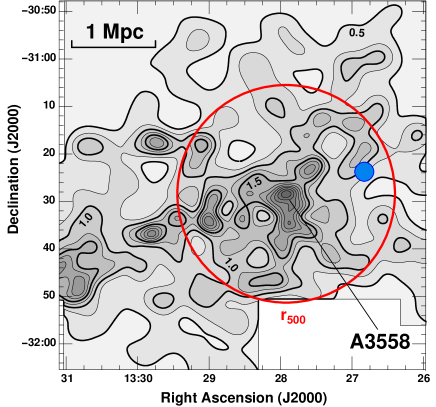
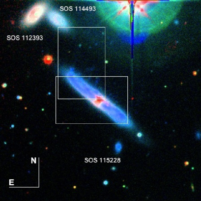
Figure 1: Left: The position of SOS 114372 is marked (blue dot) in the field of A 3558 (North up, East left) where the surface density of $R{<}2$1.0 galaxies from the SOS is shown in gray scale (from 0.33 to 2.0 galaxies arcmin^-2). The $r_{500}$ cluster radius is indicated by the red circle. Right: $BRK$ composite image of SOS 114372. The two white rectangles denote the WiFeS pointings: #1 centred on the galaxy, #2 covering the NE side. The two galaxies to the NE are supercluster members: SOS 114493 ($z$=0.05) and SOS 112393 (z=0.046). SW of SOS 114372 is a faint galaxy, SOS 115228, without redshift measurement. The orientation is indicated and adopted for all the following galaxy maps. The white bars indicating the orientation correspond to a length of 15 kpc. Channels R, G, B are assigned to $K$, $R$, $B$ bands, respectively. The nuclear region appears to be highly obscured by dust.

In Sect. 2 we describe the target. The details of IFS observations and data reduction are given in Sect. 3 and the data analysis is described in Sect. 5. The narrow-band H$\alpha$ imaging obtained using the
MMTF are presented in Sect. 4. We present the results in Sect. 6 where the morphology of ionized gas, gas and stellar kinematics and the dust attenuation map are analysed. The physical properties of the gas and the star formation across the galaxy are discussed in Sect. 7. All our findings strongly suggest the occurrence of RPS as outlined in Sect. 8 where the nature of the gas outflow is discussed considering also other possible causes as galactic winds and tidal interactions. The RPS is confirmed in Sect. 9 by ad hoc hydrodynamical simulations. We summarize the results and draw conclusions in Sect. 10.

Throughout the paper we adopt a cosmology with $\Omega_{M}$=0.3, $\Omega_{\Lambda}$= 0.7, and H₀=70 km s^-1Mpc^-1. According to this cosmology 1 arcsec corresponds to
0.941 kpc at $z$=0.048 and the distance modulus is 36.66.

Table 1: Properties of the galaxy SOS 114372.

Property	Value	Source
Magnitudes and fluxes
FUVa (1510 Å)	17.11${\pm}$0.05	Paper II
NUVa (2310 Å)	16.68${\pm}$0.03	Paper II
$B^{b}$	15.16${\pm}$0.04	Mercurio et al. 2006
$R^{b}$	14.27${\pm}$0.04	Mercurio et al. 2006
$K^{b}$	11.504$\pm$0.015	Paper I
24$\mu$m	$42{\pm}2$ mJy	Paper II
70$\mu$m	$0.758{\pm}0.038$ Jy	Paper II
90$\mu$m	$0.837{\pm}0.086$ Jy	Murakami et al. 2007
100$\mu$m	$1.2{\pm}0.2$ Jy	Allen et al. 1991
1.4GHz	9.31 mJy	Miller 2005
$K$-band bulge-disc decomposition
disc radial scale length ($r_{d}$)	5.3 arcsec	this paper
bulge effective radius	1.5 arcsec	this paper
Sérsic index of the bulge	1.2	this paper
bulge-to-disc ratio	0.44	this paper
disc inclination	82∘	this paper
Velocities
rotation velocity at $r_{d}$	200$\pm$13 km s-1	this paper
radial velocityc	826$\pm$13 km s-1	Dale et al. 1999; Proust et al. 2006
Masses
Stellar mass	7.0${\pm}0.7{\cdot}10^{10}$M⊙	Paper I
Dynamical massd	$2{\cdot}10^{11}$ M⊙	this paper
Total halo mass	$1.2{\cdot}10^{12}$ M⊙	this paper
Distances
Redshift	0.0506	Dale et al. 1999
Projected distance to cluster centre	0.995 Mpc	Sanderson & Ponman 2010
Star formation rates
Global SFR from UV+IR	8.53${}^{+2.55}_{-1.52}$ M⊙yr-1	Paper II
Global SFR from H$\alpha$	7.2$\pm 2.2$ M⊙yr-1	this paper
a) AB photometric system.
b) Vega photometric system.
c) With respect to the cluster systemic velocity.
d) Within 20 kpc radius.

2 The galaxy SOS 114372

The galaxy SOS 114372, named following the Shapley Optical Survey (SOS) identification (Mercurio et al. 2006; Haines et al. 2006), is a bright (L$\mathrel{\hbox{\hbox to0.0pt{\hbox{\lower 4.0pt\hbox{$\sim$}}\hss}\hbox{$>$}}}$L^⋆, $K$=11.504$\pm$0.015) spiral galaxy at redshift $z$=0.0506 (Dale et al., 1999) belonging to the rich cluster A 3558 (Abell richness 4) which has a median redshift $z$=0.0477 (Smith et al., 2004; Proust et al., 2006) and a velocity dispersion of 1010 km s^-1 (Proust et al., 2006). SOS 114372 is almost edge-on and is located at the projected distance of 0.995 Mpc from the centre of the cluster A 3558, well within the cluster radius
r₅₀₀=1.214$\pm$0.044 Mpc (see Sanderson & Ponman 2010) and in a relatively low-density region ($\rho$=0.88 gals arcmin^-2) as measured from the SOS $R<21$ galaxies (Fig. 1, left panel). This density is less than half of the peak density observed in the core of A 3558.

The main properties of the galaxy are listed in Table 2. The galaxy is amongst the brightest SSC members in the infra-red and it is also the brightest SSC galaxy in the ultra-violet (UV) (see Table 2 Haines et al. 2011a, hereafter Paper II), providing evidence of the presence of both obscured and unobscured star formation. The total infra-red luminosity of the galaxy is estimated as $L_{TIR}{=}1.1{\pm}0.1{\cdot}10^{11}L_{\odot}$ based on fitting the infra-red SED models of Rieke et al. (2009) to the Spitzer/MIPS 70$\mu$m flux and AKARI 90$\mu$m flux (Murakami et al., 2007). These data are also consistent with the prior IRAS 100$\mu$m flux measurement (Allen et al., 1991). Miller (2005) measured a radio flux at 1.4GHz of 9.31 mJy corresponding to a luminosity L${}_{1.4GHz}{=}5.3{\cdot}10^{22}$W Hz^-1, consistent with expectations from the FIR–radio correlation in which both the FIR and radio emissions come from ongoing star formation (Paper III). Following Leroy et al. (2008), we estimated a global SFR=8.53${}^{+2.55}_{-1.52}$ M_⊙yr^-1 (of which 78% is obscured, Paper II) with the errors accounting for the SFR calibration uncertainty. The most intense star formation occurs in the heavily obscured centre, but an intense region of less-obscured star formation is also observed in the SW disc (see Sect. 6.3).

We estimate a stellar mass of $\mathcal{M}_{\star}{=}7.0{\pm}0.7{\cdot}10^{10}$M_⊙ (Paper I). SOS 114372 has dynamical mass within 20 kpc radius of $\mathcal{M}_{dyn}{\sim}2{\cdot}10^{11}$ M_⊙ (see Sect.6.2) from which we can estimate the total halo mass following Conselice et al. (2005) of $\mathcal{M}{=}1.2{\cdot}10^{12}$ M_⊙. To derive the structural properties of the galaxy, we modelled the light distribution in $K$ band with a Sérsic profile for the bulge plus an exponential disc using GALFIT (Peng et al., 2010). The choice of the $K$-band allows to mitigate the effect of strong dust absorption. The disc radial scale length is $r_{d}$=6.4 arcsec ($\simeq 6$ kpc) which, after applying the “dust correction” introduced by Graham & Worley (2008) becomes $r_{d}\simeq 5.3$ kpc. The effective radius of the ‘bulge’ is $r_{e}$=1.5 arcsec ($\simeq 1.4$ kpc). The ‘bulge’ is significantly elongated, with an axis ratio of 0.7, is tilted with respect to the disc by 13^∘, and its Sérsic index is n=1.2 indicating that it is actually a bar. The disc axis ratio is 0.14, which implies an inclination of the disc with respect to the line of sight of 82^∘. The $K$-band bulge-to-disc ratio is B/D=0.44, after correcting for inclination following Driver et al. (2008).

The $BRK$ composite image, as derived from the SOS (ESO-WFI, Mercurio et al, 2006) and $K$-band surveys (UKIRT-WFCAM, Paper I), shows evidence of dust absorption in and SE of the galaxy centre (Fig. 1, right panel). In the composite image we also notice hints of matter beyond the stellar disc (north-west from the disc, see Sect. 6). The orientation of Fig. 1 with North upwards and East to the left will be adopted throughout the article.

3 Integral-field spectroscopy

3.1 Observations

The spectroscopic data of SOS 114372 were obtained during two observing runs in April 2010 (pointing #1) and April 2011 (pointing #2) using the Wide-Field Spectrograph (WiFeS; Dopita et al. 2007, 2010) on the Australian National University 2.3m telescope at the Siding Spring Observatory, Australia. WiFeS is an image-slicing integral-field spectrograph that records optical spectra over a contiguous 25^′′$\times$ 38^′′ field-of-view. This field is divided into twenty-five 1^′′-wide long-slits (‘slices’) of 3$8^{\prime\prime}$ length. The spectra were acquired in ‘binned mode’, with 25$\times$38 spaxels of 1${}^{\prime\prime}\times$ 1^′′ size. Hereafter we will refer to the spatial directions across the slices or along them as ‘X’ or ‘Y’ direction respectively. WiFeS has two independent channels for the blue and the red wavelength ranges. We used the B3000 and R3000 gratings, allowing simultaneous observations of the spectral range from $\sim$3300 Å to $\sim$9300 Å with an average resolution of R=2900. For further details on the WiFeS instrument see Dopita et al. (2007, 2010).

The positions of the WiFeS field-of-view for the two pointings are shown in Fig. 1 (right panel). The total integration time on the galaxy was of 4.5 h in run #1, obtained as the sum of 6$\times$45 min exposures. Pointing #2 was obtained to map the gas distribution in the Northern side of the galaxy and to measure the extent of extraplanar gas. The data of this pointing are shallower (2$\times$45 min) than run #1 and are used to map the gas and derive the kinematics, but not to measure line flux ratios. For each galaxy spectrum, we also acquired the spectrum of a nearby empty sky region with 22.5 min exposure to provide accurate sky subtraction.

For each galaxy exposure we obtained spectra of spectrophotometric standard stars for flux calibration and stars with nearly featureless spectra to monitor the atmospheric absorption bands. Arc and bias frames (see below) were also taken for each science exposure. Internal lamp flat fields and sky flats were taken twice during both runs.

3.2 Data reduction

The data were reduced using the WiFeS data reduction pipeline (Dopita et al., 2010) and purposely written FORTRAN and IDL codes. The WiFeS pipeline performs all the steps from bias subtraction to the production of wavelength- and flux-calibrated data-cubes for each of the $B$ and $R$ channels. The average r.m.s. scatter around the dispersion relation was 0.2–0.3 Å. The final spectral resolution achieved is $\sigma{\sim}40$ km s^-1, and is wavelength and position dependent (see below). The data-cubes were sampled at 1^′′$\times$1^′′$\times$1 Å and cover a useful wavelength range of 3600–9000 Å. The data-cubes are also corrected for atmospheric differential refraction.

Accurate sky subtraction is particularly important for our data because of the presence of OH lines in the vicinity of the H$\alpha$ line and the [Nii] doublet at the redshift of the SSC. Sky subtraction was carried out as follows. The sky spectrum taken closest in time to the galaxy spectrum was first cleaned of cosmic ray hits using the code LACosmic (van Dokkum, 2001) to detect them, followed by an interpolation along the spatial direction to remove them. The sky spectra were then smoothed in the Y direction with a median filter. This allowed us to effectively minimize the introduction of noise in sky subtraction. In an ideal case, we should have multiplied the sky cubes by a factor of two (the ratio of exposure times) before subtraction, but due to differences in airmass and changes in sky conditions, especially affecting the amplitudes of emission lines, we normalized the sky frames to the galaxy frames by comparing the relative strengths of the atmospheric emission lines. This resulted in a range of multiplicative factors for the sky frames (${\sim}1$.5–2.5).

Particular attention was devoted to the removal of the atmospheric absorption features, since at the redshift of the SSC the atmospheric band at $\sim$6870 Å may affect the [Nii]-H$\alpha$ group. This O₂ band is accompanied by two other O₂ bands ($\sim$ 6280 Å and $\sim$ 7600 Å ) which could be effectively used to monitor the quality of the subtraction.

The co-addition of the individual exposures requires an accurate spatial registration of the data-cubes. For this purpose, we took advantage of the high quality ESO-2.2m WFI $B$- and $R$-band images of the galaxy from the SOS. The bandpasses of these images can be matched to the $B$ and $R$ channels of WiFeS. The true spatial scale of WiFeS data was determined from (i) the distance between the galaxy nucleus and a star taken during run #1 and (ii) images of the centre of the globular cluster NGC 3201 acquired in run #2 for this purpose. We find that while the X scale of WiFeS is 1^′′/pixel, the Y scale is larger than the nominal 0.5^′′/pixel by a factor 1.15 for the $B$ data-cube and 1.04 for the $R$ data-cube. After correcting for these pixel scales we multiplied the WiFeS cubes with the WFI response curves and determined the relative spatial position by cross-correlation. The individual exposures were then registered and co-added using IRAF. $B$ and $R$ fluxes were adjusted, where necessary, by matching the fluxes in the common wavelength range (5300–5600 Å ). The adjustment required was always within the estimated flux errors (see Sect. 5.2). The reduced data-cubes were finally corrected for Galactic extinction following Schlegel et al. (1998) and using the extinction curve by Cardelli et al. (1989) with R_V=3.1. The sensitivity of our data turns out to be 0.5$\cdot$10^-17erg s^-1cm^-2Å^-1 arcsec^-2 at a signal-to-noise ratio SNR=5. This is the lowest SNR for which we consider our measurements reliable.

4 H$\alpha$ imaging

Deep H$\alpha$ imaging of the galaxy SOS 114372 was obtained with the Maryland-Magellan Tunable Filter (MMTF; Veilleux et al., 2010) on the Magellan-Baade 6.5m telescope at the Las Campanas Observatory in Chile on 20 May 2012. The MMTF is based on a Fabry-Perot etalon, which provides a very narrow transmission bandpass (${\sim}$5–12Å) that can be tuned to any wavelength over ${\sim}5$000–9200Å (Veilleux et al., 2010). Coupled with the exquisite image quality provided by active optics on Magellan and the Inamori-Magellan Areal Camera & Spectrograph (IMACS), this instrument is ideal for detecting extra-galactic H$\alpha$-emitting gas. The MMTF 6815-216 order-blocking filter with central wavelength of 6815Å and FWHM of 216Å was used to provide coverage of the H$\alpha$ emission line for galaxies belonging to the Shapley supercluster.

At the start of the observing run the etalon plates were parallelized and the wavelength calibration of the etalon for our setup was determined and further checked throughout the night. The MMTF does not provide a monochromatic image over the full extent of the IMACS $27^{\prime}{\times}27^{\prime}$ field of view, but rather a central circular monochromatic region (the Jacquinot spot), outside of which the central transmission wavelength monotonically decreases with increasing angular distance from the optical axis in a well understood manner. The instrumental set-up was chosen to provide the largest Jacquinot spot (${\sim}11.5^{\prime}$) and a transmission bandpass of FWHM 10.3Å (corresponding to ${\sim}4$70 km s^-1). The target galaxy was always placed at the same location, well within the Jacquinot spot, but away from the gaps between CCDs.

The galaxy was observed for a total 60 minutes in H$\alpha$ ($4{\times}900$ sec). The galaxy was also observed for 15 minutes in the continuum, by shifting the central wavelength of the etalon ${\sim}5$0Å bluewards to exclude emission from both the H$\alpha$ line and the adjacent [Nii] lines, and into a wavelength region devoid of major skylines. The typical image resolution for these exposures was $0^{\prime\prime}.50$.

These data were fully reduced using the MMTF data reduction pipeline, which performs bias subtraction, flat fielding, sky-line removal, cosmic-ray removal, astrometric calibration and stacking of multiple exposures (see Veilleux et al., 2010). Photometric calibration was performed by comparing the narrow-band fluxes from continuum-dominated sources with their known $R$-band magnitudes obtained from our existing WFI images. Conditions were photometric throughout and the error associated with our absolute photometric calibration is ${\sim}10$%. The effective bandpass of the Lorenzian profile of the tunable filter of ${\pi}/2{\times}$FWHM is then used to convert the observed measurements into $H{\alpha}$ fluxes in units of erg sec^-1 cm^-2. The filter is sufficiently narrow that there should be little or no contamination from [Nii] emission. The data were obtained in dark time resulting in very low sky background levels, with 1$\sigma$ surface brightness fluctuations within a 1 arcsec diameter aperture of $0.2{\times}10^{-17}$ erg s^-1 cm^-2Å^-1 arcsec^-2 implying a sensitivity of
1.0$\times$10^-17 erg s^-1 cm^-2Å^-1 arcsec^-2 at SNR=5.

5 Data analysis

In this section we describe the stellar continuum modeling and the measurement of the emission line fluxes. The emission-line fluxes are used to estimate: i) the gas kinematics (Sect. 6.2); and in each galaxy region ii) the line diagnostics (Sect. 7.1); iii) the dust attenuation for the ionized gas and SFR across the galaxy (Sects. 6.3 and 7.2). The stellar continuum modeling is needed to obtain the pure emission-line spectrum and, accounting for the dust extinction, allow us to infer stellar population ages in different galaxy regions (Sect. 7.2).

5.1 Stellar continuum modeling and subtraction

Late-type galaxies present complex star formation histories with continuous bursts of star formation from the earliest epochs right up until the present day (Kennicutt, 1983; Kennicutt et al., 1994; James et al., 2008; Williams et al., 2011). This implies that, unlike early-type galaxies, their spectra and absorption line indices cannot be successfully fit by comparison to those from single stellar population models. Instead the technique of full spectral modeling has been developed to reliably describe the properties of the individual stellar components (Cid Fernandes et al., 2005; Ocvirk et al., 2006; Koleva et al., 2009; MacArthur et al., 2009). This involves the fitting of spectra over extended wavelength ranges (i.e. not just absorption lines) by linear combinations of multiple stellar populations, while also accounting for the impact of line-of-sight stellar motions and instrument resolution, and the non-linear effects of dust extinction. A variety of implementations of full spectral fitting have been developed, which explicitly attempt to derive robust stellar population parameters and their uncertainties, including the use of detailed simulations (e.g. Cid Fernandes et al., 2005; Koleva et al., 2008, 2009).

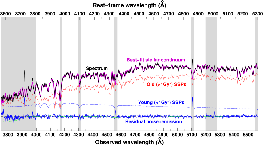
Figure 2: Example result from the stellar continuum fitting process. The black curve shows the input spectrum, coming from the 3x3 spaxels region, centred on the photometric centre of the galaxy. The magenta curve shows the resultant best-fit stellar continuum comprising a linear combination of SSPs, requiring both old ($>1$ Gyr; thin red curve) and young ($<1$ Gyr old; thin blue curve) components. The shaded regions indicate the wavelength ranges excluded from the fitting process, including the masks for emission lines. The residual emission component (thick blue curve) reveals clear emission at [Oii] $\lambda 3729$, H$\delta$, H$\gamma$, H$\beta$ and [Oiii] $\lambda\lambda\,4959\,5007$.

To obtain a reasonable fit to the stellar continuum a signal-to-noise level of ${\mathrel{\hbox{\hbox to0.0pt{\hbox{\lower 4.0pt\hbox{$\sim$}}\hss}\hbox{$>$}}}}5$0/Å is generally required (e.g. Sánchez et al. 2011). We take for each spaxel the continuum from the $3{\times}3$ region centred on the spaxel, which for the main body of the galaxy was sufficient to achieve the necessary signal-to-noise. Outside the galaxy disc, further smoothing was required, and so increasingly large rectangular regions centred on the spaxel were considered until a mean signal-to-noise level of ${\sim}40$/Å was reached for the stellar continuum over the wavelength range 4600–4800 Å.

For each spaxel, the spatially-smoothed spectrum from the blue arm is firstly fit with the Vazdekis et al. (2010) stellar population synthesis models. We mask out regions below 3950 Å which have significantly reduced signal-to-noise levels and flux calibration reliability, and above 5550 Å where a bright sky line is located. The wavelength regions affected by emission lines are also masked out.

We consider a total of 40 simple stellar populations (SSP) models covering the full range of stellar ages (0.06–15 Gyr) and three different metallicities [M/H]=–0.41, 0.0, +0.22. The majority of SSP models had solar metallicity and provided the required fine sampling of age, while additional evolved (1–15 Gyr old) super-solar models were included to improve the fitting of the small-scale continuum features. The models assume a Kroupa (2001) initial mass function (IMF). The Vazdekis et al. (2010) SEDs, based on the Medium resolution INT Library of Empirical Spectra (MILES) of Sánchez-Blázquez et al. (2006), have a nominal resolution of 2.3 Å, close to our instrumental resolution, and cover the spectral range 3540–7410 Å.

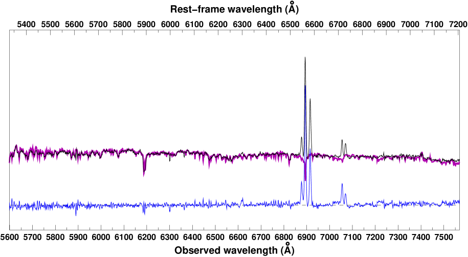
Figure 3: Example of the stellar continuum modeling in the red arm. The black curve shows the red-arm spectrum, coming from the same 3$\times$3 spaxel region as Fig. 2, which is located in the core of the galaxy. The magenta curve shows the resultant best-fit stellar continuum comprising a linear combination of SSPs, based solely on the fit to the blue arm, and extrapolated to the red arm. The blue curve shows the residual emission, i.e. subtracting the magenta curve from the black curve. Notice the emission lines of [Oi], H$\alpha$, [Nii], [Sii] at the observed wavelengths 6620Å, 6895Å, 6880-6917Å, 7057-7072Å.

In a first pass, the best-fitting Vazdekis et al. SSP is taken to derive the absorption-line redshift, $z_{abs}$, and subsequently a first estimate of the velocity dispersion, $\sigma$, assumed to be in the range 0–300 km $s^{-1}$. The value of $\sigma$ can be strongly affected by template mismatch, and so it is important that the full range of SSP models are fitted over. The $\sigma$ is determined as that which minimizes the $\chi^{2}$ value for all combinations of $\sigma$ and SSP model. We then fix the values of $z_{abs}$ and $\sigma$, and iteratively fit the observed spectrum by a non-negative linear combination of the 40 SSPs in order to minimize the $\chi^{2}$ value, until convergence is reached. Throughout this iterative process, individual strongly discrepant pixels (${>}5{\sigma}$) are identified and masked if necessary, to ensure that single pixels do not bias the convergence of the fit. This final linear combination is typically found to be composed of 8–10 individual stellar populations. A final fit to estimate $\sigma$ is made using the best-fit complex stellar population model. The final linear combination of SSPs is then re-scaled linearly to obtain the best-fit to the spectrum from the single central spaxel and then subtracted to obtain the pure emission spectrum for that spaxel corrected for stellar absorption. We neglect internal extinction in this continuum fitting process, since our aim here is to fit the stellar continuum in order to model and subtract it in the regions of the emission lines, while we include dust extinction in our later star formation history analysis limited to three galaxy regions (Sect. 7.2).

Following Moustakas et al. (2010), any remaining residuals (typically of the order a few percent), due to imperfect sky subtraction, or template mismatch, are removed using a 25-pixel sliding median (again masking out the emission lines). This last stage had little impact on the residual spectrum, except for the extreme blue end with $\lambda{<}3800$ Å, where the flux calibration accuracy is weakest, and the additional masking of emission lines, ensured that it did not impact the final emission line measurements.

Having fit the stellar continuum for the blue arm spectrum, this best-fit linear combination of SSPs is taken and extended into the red arm. Then varying only the global scaling factor to account for any (slight) mismatch in the flux calibration between red and blue arms, it is subtracted from the red arm spectrum, to produce the pure emission spectrum for the corresponding spaxel in the red arm.

In Fig. 2 we show an example output of our stellar continuum fitting process. The input spectrum (black curve) is from a 3$\times$3 spaxels region in the centre of the galaxy. The resultant best-fit stellar continuum (magenta curve) comprising a linear combination of SSPs, requires both young and old (thin blue/red curves) components. Almost all of the small-scale structures seen in the observed spectrum are real rather than noise, being precisely mapped by the model stellar continuum. The shaded regions correspond to wavelength ranges not considered in the fitting process, including the masks for emission lines. This stellar continuum is subtracted from the observed spectrum to produce the residual emission component (thick blue curve) accounting now for stellar absorption, revealing clear emission at Oii, H$\delta$, H$\gamma$, H$\beta$ and [Oiii]. The Balmer emission lines are all located within deep absorption features, demonstrating the necessity of accurately modeling and subtracting the stellar continuum prior to measuring these lines. Outside of the emission lines, the rms levels in the residual signal are consistent with expectations from photon noise, with little remaining structure. This holds true throughout the galaxy indicating that on a spaxel-by-spaxel basis the model fits to the stellar continuum are formally good ($\chi^{2}_{\nu}{\sim}1$). Figure 3 shows the fit extended in the red arm for the same spatial region as Fig. 2. The SSP model continuum (thick magenta curve) of the spectrum (black curve) is able to describe all the absorption features and once subtracted (blue curve) allows robust emission line measurements.

5.2 Emission-line measurements

Emission-line fluxes and widths were measured with a purposely written FORTRAN code, which performs a Gaussian fit to the emission lines. Where lines are either partially overlapping or close (as for the groups [Nii]-H$\alpha$-[Nii], [Sii]6717-6731 and [Oiii]4959-5007), the lines are fitted simultaneously. The fits are however left completely independent even in the case when their flux ratios are known to be fixed. This was done to assess the reliability of our measurements (see below). The code first fits a straight line to the residual continuum (after sky subtraction and stellar population fitting and subtraction) on either side of the line, and then fits a Gaussian to each continuum-subtracted line to derive the position of the maximum, the peak amplitude, and dispersion $\sigma$. These values are then used to perform a series of (50) simulations in which random scatter derived from the continuum fit is added to the solution, and these simulated lines are fitted again. The standard deviation of the distribution of the fitting parameters is then adopted as the contribution of the fit to the uncertainty. Fluxes are computed from the measured amplitudes and $\sigma$.

We estimate the SNR of the emission as being the ratio of the peak amplitude to the standard deviation of the surrounding continuum. Comparing the SNR with the error coming from the fit and taking into account the appearance of the lines, we fix at SNR=5 the lower limit for reliable measurements. This limit corresponds to $\sim$30% relative errors from the fit for both the flux and $\sigma$. The total error on the flux is computed adding in quadrature the uncertainty in the flux zero-point, estimated comparing the fluxes of the individual exposures taken in good atmospheric conditions. This amounts to $\sim$7% –10% ($R$ and $B$ respectively).

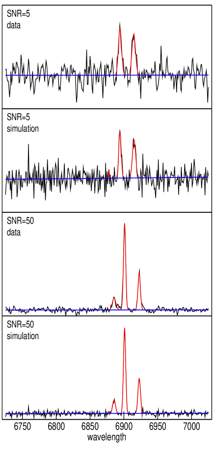
Figure 4: Measurement of the emission lines in the group [Nii]-H$\alpha$-[Nii] for two values of SNR of H$\alpha$. From top to bottom the real data and one of the simulation in a spaxel with SNR$\sim 5$ (first two plots) and in a spaxel with SNR$\sim 50$ (last two plots). The black curves are the observed and simulated spectra, while the red curves are the fits to the emission lines and the continuous lines are the fits to the continuum. SNR=50 is the mean value of our data.

Figure 4 shows examples of both real and simulated data, and the computed fits in the case of SNR$\sim$5 (our lower limit) and SNR$\sim$50 (the average of our data) in the wavelength region around H${\alpha}$.

The instrumental contribution to the line widths was estimated by measuring the widths of selected arc-lamp lines from the $B$ and $R$ data-cubes. Due to the combination of spherical aberration and high-order astigmatism in the instrumental point spread function, the instrumental line width $\sigma_{instr}$ depends on the wavelength and on the X spatial direction, but not on the Y direction. We constructed maps of $\sigma_{instr}(X,\lambda)$ which were subtracted in quadrature from the data to obtain the intrinsic velocity dispersion of the gas. At our observed wavelength of H$\alpha$ (${\sim}6$800 Å), $\sigma_{instr}{\sim}5$1–62 km s^-1, being close to the maximum in the centre of the field. The total error on the velocity dispersion accounts for the uncertainty of ${\sim}5$ km s^-1 in $\sigma_{instr}$. The errors from the fit on radial velocity are very small (${<}5$ km s^-1), so the main contribution comes from the uncertainty in wavelength calibration, which is ${\sim}13$ km s^-1.

As explained above, we chose to measure all lines independently in order to be able to assess the reliability of our flux ratios. With this aim, we compared our measurements of the [Nii] $\lambda\lambda$6583/6548 and [Oiii] $\lambda\lambda$4959/5007 line ratios to their theoretical values of 2.976 (Dopita & Sutherland, 2003) and 2.936 (Storey & Zeippen, 2000), respectively. We found that for an error on the flux ratio less than 30%, the involved lines must have at least SNR$>$10 (consistent with the above errors on the individual fluxes), and adopted a more conservative limit of SNR$>$20.

To achieve this SNR, we applied a spatial adaptive binning to our data by means of the ‘Weighted Voronoi Tessellation’ (WVT) by Diehl and Statler (2006), which is a generalization of the algorithm that Cappellari & Copin (2003) developed for SAURON data. The WVT performs the partitioning of a region based on a set of points called ‘generators’, the points around which the partition of the plane takes place. The partitioning is repeated iteratively until some target SNR is achieved in all bins. The WVT algorithm allows to ‘manually’ set a number of generators, which we chose on the basis of the position with respect to the stellar disc. We obtained a total of 104 regions. As input data we used the signal and noise of the H$\alpha$ emission line, which has the widest spatial coverage. The faintest line involved in our flux ratios is the [Oi] $\lambda$6300 line, whose flux is typically about $\sim 20$% of H$\alpha$, so that we set SNR=100 for H$\alpha$ as the target SNR for the WVT algorithm in order to achieve the required SNR for the [Oi] line. The WVT is adopted to derive flux ratios, dust attenuation, and SFR, but not for the kinematics, for which no spatial binning was necessary.

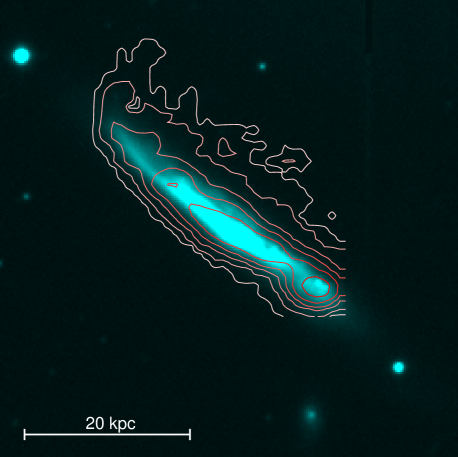
Figure 5: Logarithmically-spaced contours of H$\alpha$ flux in the range 5$\cdot$10^-18– 5$\cdot$10^-16erg cm^-2s^-1Å^-1arcsec^-2 from WiFeS are superimposed on the ESO-WFI $R$-band image of the galaxy. Extraplanar gas is visible out of the disc in the NW (upper right). The scale is shown on the bottom. The H$\alpha$ flux was corrected for dust attenuation (Sect. 6.3).

6 Results

Figure 5 shows the contours of the H$\alpha$ emission-line flux from WiFeS tracing the ionized gas superimposed on ESO-WFI $R$-band image. The ionized gas extends for about 13 kpc in projection out of the galaxy disc in the NW direction. No gas is detected beyond that distance, although pointing #2 covers further 13 kpc North from the most external gas isophote in Fig. 5. In order to understand the origin of the extraplanar gas, we examine the structure and morphology of the ionized gas, derived the gas and stellar kinematics and the dust extinction across the galaxy.

6.1 Morphology of the H$\alpha$ emission

The H$\alpha$ narrow-band image allows us to resolve the structure of the extraplanar gas. Fig. 6 shows the MMTF H$\alpha$ image (white) combined with the UKIRT $K$-band (red) image (left panel) and with the contours of H$\alpha$ flux measured with WiFeS (right panel). The most noticeable feature of the H$\alpha$ image are the compact (${\mathrel{\hbox{\hbox to0.0pt{\hbox{\lower 4.0pt\hbox{$\sim$}}\hss}\hbox{$<$}}}}0.5^{\prime\prime}$; ${\mathrel{\hbox{\hbox to0.0pt{\hbox{\lower 4.0pt\hbox{$\sim$}}\hss}\hbox{$<$}}}}500$ pc) knots of H$\alpha$ emission seen all along the NW side of the disc. Some of these knots seem “tethered” to the disc by faint filamentary strands. The most distant knot is seen at $\sim$13 kpc (in projection) from the galaxy major axis, but most knots are much closer, within 3–4 kpc of the disc. All of these knots and filamentary structures are completely absent in the MMTF continuum image, confirming that this is from H$\alpha$ emission with little if any underlying stellar continuum component. It is notable that there are no such H-alpha features on the SE side.

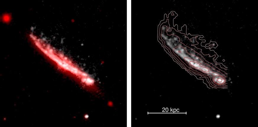
Figure 6: Left: Composite image of SOS 114372 consisting of the MMTF H$\alpha$ image (white) over the UKIRT $K$-band image (red). SOS 115228 is seen as the white spot closest to the bottom. The H$\alpha$ flux is not corrected for dust attenuation. Right: Contours of H$\alpha$ flux measured with WiFeS over the MMTF H$\alpha$ image. The scale for the two panels is indicated.

The most luminous knot has an H$\alpha$ luminosity of $7.2{\times}10^{38}$ erg s^-1, while the faintest detected knots have $L(H{\alpha}){\sim}1.5{\times}10^{38}$ erg s^-1. If all of this emission were powered by star formation, these luminosities would correspond to SFRs of 0.0008–0.004 M_⊙ yr^-1 based on the calibration of Kennicutt (1998) with a Kroupa IMF (see Sect. 7.1). A bright, clumpy H$\alpha$-emitting region ${\sim}$6 kpc in extent is located in the disc $\sim$12 kpc SW of the galaxy centre, indicative of a localized ongoing starburst (see Sect. 6.3).

The small galaxy SOS 115228 (Fig 1, right) SE of SOS 114372 has also an H$\alpha$-emitting region associated with it, which appears ${\sim}2.8{\times}$ brighter in our MMTF H$\alpha$ filter than the continuum filter. Although SOS 115228 does not have a known redshift, this might be suggestive of a starbursting dwarf galaxy at the same redshift (within ${\sim}400$ km s^-1) as
SOS 114372. Although clearly compact, SOS 115228 does not appear as a point source in H$\alpha$, but likely has an intrinsic diameter of ${\sim}0.35^{\prime\prime}$ (350 pc). Alternatively, SOS 115228 could be a much more distant active (starburst or AGN) galaxy whose H$\beta$ emission happens to be detected in our MMTF image. The redshift of this galaxy would then be z$\sim$0.42. This difference in redshift would be consistent with the $\sim$5 mag difference in $K$-band magnitude with SOS 114372, if the two galaxies have comparable masses. Unfortunately, no conclusion can be drawn on the nature of this object without spectroscopic data.

6.2 Gas and stellar kinematics

The gas velocity field derived from IFS observations is shown in Fig. 7 (left panel). The white contours trace the $R$-band stellar continuum derived from the spectrum once the emission lines have been removed. The dashed lines mark the major and minor axes of the disc extending to 3$\times r_{d}$, and cross at the $K$-band photometric centre. The black curves are iso-velocity contours. The kinematic centre is assumed to coincide with the photometric centre of the $K$-band image. It turns out that this choice also produces the smallest asymmetries in the major axis kinematic profile.

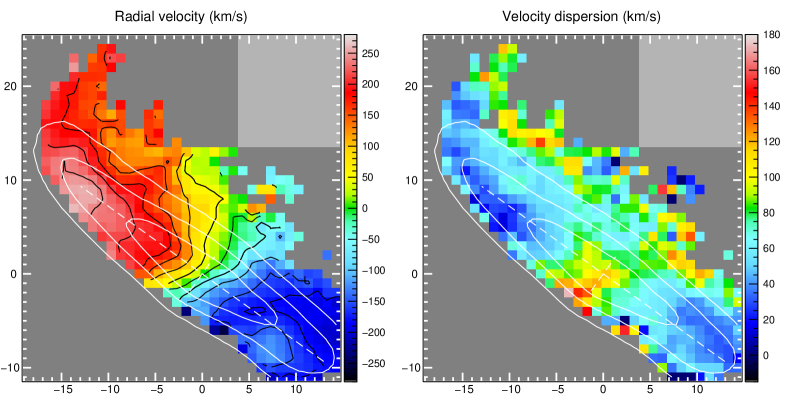
Figure 7: Gas kinematics of SOS 114372 derived from the fit to the H$\alpha$ emission line. The light gray rectangle marks the region not covered by the two pointings. The white iso-density contours trace the galaxy red continuum and the dashed lines, extending to 3$\times r_{d}$, show the positions of the minor and major axis and cross at the $K$-band photometric centre. Left: Gas velocity field. Each pixel is colour coded according to the measured radial velocity relative to the galaxy centre. The black curves are iso-velocity contours. Right: Gas velocity dispersion. Each pixel is colour coded according to the measured velocity dispersion. In this figure and in the following maps the ticks on the axes indicate the apparent distance from the $K$-band photometric centre in arcsecs. The velocity scales are on the right of each panel.

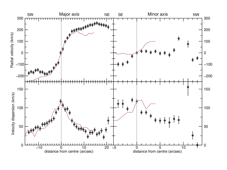
Figure 8: Gas line-of-sight velocity (upper panels) and velocity dispersion (lower panels) profiles along the major (left panels) and minor axis (right panels). The red lines represent the same data reflected with respect to the origin, to facilitate the inspection of asymmetries. Distances from the photometric centre are positive towards NE (major axis) and NW for the minor axis. Directions in the sky are given on the top of the figure.

The velocity field is complex. Within the disc, the overall appearance of the field is that of a rotating disc, although significant departures from a simple rotation are present everywhere, as it is also clearly shown in the radial velocity profiles along the major and minor axes (Fig. 8).

The major axis velocity profile (Fig. 8) is fairly symmetric in the inner $\sim$5 arsec. Beyond that radius, the radial velocity in the NE side of the disc increases until it reaches $\sim$250 km s^-1 at $\sim$16 arcsec from the centre and then it starts decreasing until the last observed point at 21 arcsec. In the SW side, the absolute value of the velocity first decreases to a local minimum of $\sim$140 km s^-1 at 10 arcsec from the centre and then slightly increases until the last observed point. The whole situation depicted in Fig. 7 is even more complex than this, as is immediately clear from the shape of the iso-velocity contours. The velocity field in the disc is asymmetric also with respect to the minor axis, with the SE side of the disc generally more red-shifted than the NW side. There are two local maxima in the SE side, one at $\sim$3 $r_{d}$ NE from the centre and one at $\sim$2 $r_{d}$ SW from it. The kinematics of the extraplanar gas appears to be remarkably dominated by the rotation characterising the disc, maintaining the iso-velocity contours continuous up to the most external limits. We notice that, NE from the galaxy centre, the extraplanar gas is in the average blue-shifted with respect to the nearest gas in the disc, while in the SW it is red-shifted, thus producing ’fan-shaped’ iso-velocity contours. The minor axis radial velocity profile allows us to identify a gas stream approaching the observer, reaching a velocity of $\sim$100 km s^-1 at $\sim$3-4 arcsec SE from the nucleus.

From the major axis radial velocity profile we derive a dynamical mass within 20 kpc of $\mathcal{M}_{dyn}{=}2.1{\cdot}10^{11}$M_⊙.

The gas velocity dispersion field is also quite complex (Fig. 7; right panel). We first notice that the velocity dispersion $\sigma$ rarely reaches values as small as would be expected in normal turbulent HII regions ($\sigma{\sim}2$0–30 km s^-1). The velocity dispersion is particularly high ($>100$ km s^-1) over a significant fraction of the extraplanar gas. High values of $\sigma$ are also observed in two regions near the SE border of the disc. The most remarkable of the two is the triangular area with $\sigma\mathrel{\hbox{\hbox to0.0pt{\hbox{\lower 4.0pt\hbox{$\sim$}}\hss}\hbox{$>$}}}$120 km s^-1 extending SE from the nucleus, where we also measure the absolute maximum of the velocity dispersion (${\sim}$180 km s^-1). This area corresponds to the stream directed towards the observer noted above. We remark that the value of the velocity dispersion also depends on the spatial sampling of the spectrograph, increasing with pixel size and seeing, as the combination of the motions of more gas elements is measured in each resolution element. This is certainly a major origin of our average high values of $\sigma$, because it is clear from the radial velocity field that complex motions are taking place giving rise to different possible kinds of superimpositions. We notice that our resolution element of 1${}^{\prime\prime}\times 1^{\prime\prime}$ corresponds to $\sim$1$\times$7 kpc² once projected on the plane of the disc. We also remark that the presence of large quantities of obscuring dust may complicate the interpretation of the gas kinematics, since dust may selectively hide parts of the moving gas (e.g. Giovanelli & Haynes 2002; Baes et al. 2003; Kregel et al. 2004; Valotto & Giovanelli 2004), although this would probably not increase the measured velocity dispersion.

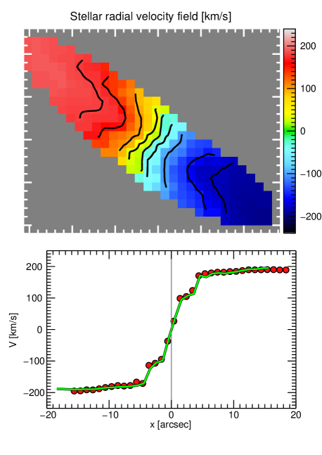
Figure 9: Top: The stellar velocity field with Iso-velocity contours. Bottom: The stellar radial velocity profile along the major axis (red dots) with its reflection with respect to the centre superimposed (green curve).

From the fit of the stellar continuum we derived the velocity field of the stars. In order to estimate the uncertainties in the stellar velocity we used simulations in which random noise is added to the spectra. A typical uncertainty of $\sim$2 km s^-1 for spaxels in the disc is found. This low uncertainty is probably due to the previous 3$\times$3 smoothing in the spatial direction. Including the uncertainty in wavelength calibration, this sums up to $\sim$14 km s^-1.

The derived stellar radial velocity field and major axis radial velocity profile are shown in Fig. 9. The iso-velocity contours of the stellar component appear symmetric with respect to the centre, while they are skewed with respect to the minor and major axis. Along the major axis, the radial velocity grows linearly and rapidly in the inner $\sim$1.5-2 arcsec, where there is an abrupt change of slope followed by another rapid increase. At $\sim$5 arcsec from the centre the radial velocity assumes an almost constant value of $\sim$180 km s^-1 until the last observed points. The kinematic centre of the stellar velocity field is displaced 0.3 arcsec (280 pc) NE with respect to the photometric ($K$ band) centre of the galaxy (and consequently to the kinematic centre of the gas). However, we will not further discuss this point, since this displacement is smaller than our resolution element.

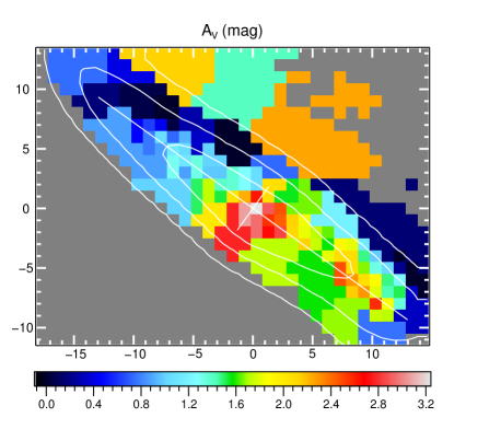
Figure 10: Dust attenuation derived from the H$\alpha$/H$\beta$ line ratio.

6.3 Dust extinction across the galaxy

Figure 10 shows the distribution of the dust attenuation derived from the H$\alpha$/H$\beta$ line ratio, in terms of the visual extinction $A_{V}$. We use the theoretical attenuation curve by Fischera & Dopita (2005) with $R_{V}{=}4.5$. The dust extinction is estimated in each of the binned region of Fig. 11. The level of dust attenuation is notably asymmetric along the major axis, being universally lower on the NE side of the disc than the SW side. The highest dust extinction ($A_{V}{\sim}2$.4–3.2 mag) is observed in the centre of the galaxy, extending along the minor axis to the SE edge. Highly attenuated regions ($A_{V}{\sim}1$.9–2.6 mag) are also found in the SW disc ${\sim}1$2 kpc from the galaxy centre and in the extraplanar gas. This extinction map agrees with what can be inferred from the optical images, where dust absorption is clear in the galaxy centre (see also Fig. 1 right panel).

7 Properties of the gas and star formation across the galaxy

Our data, complemented by available multi-band imaging (from far-UV to far-IR), allow us to investigate the nature of the gas and the star formation across the galaxy, but first we examine the gas and stellar kinematics.

The stellar kinematics is typical of a barred galaxy, with the twisting of the iso-velocity contours due to the non-circular motions induced by the bar (Athanassoula & Misiriotis, 2002) and with a ‘double-bump’ rotation curve (Chung & Bureau, 2004; Bureau & Athanassoula, 2005). A detailed analysis of the stellar kinematics is beyond our goals, since it would require much higher spatial resolution (e.g. Emsellem et al. 2007), but the important point for this work is that the stellar velocity field appears to be regular and symmetric, without any signs of perturbation. One may ask whether the regularity of the stellar kinematics field, in sharp contrast with the gas, is due to the smoothing applied to the spectra to increase the SNR of the stellar component. We verified that this is not the case by applying the same 3$\times$3 binning to the gas velocity field. The effect was just a smoothing of the small-scale features, with the gross properties remaining unchanged. This holds also for much more severe binning (up to 7$\times$7 pixels). The complexity of the gas velocity field cannot be explained by the presence of the bar alone, as can be seen by comparing the iso-velocity contours in Fig. 7 to the velocity fields of barred galaxies reported, for instance, in Bosma (1981), Courteau et al. (2003), Fathi et al. (2005) and de Naray et al. (2009). All these considerations make us to conclude that the gas kinematics is heavily perturbed, while the stellar kinematics is not.

7.1 Physical properties of the gas

The key diagnostics for the examination of the mode of excitation of an ionized plasma were introduced by Veilleux & Osterbrock (1987). These use the [Nii]/ H$\alpha\,$, [Sii]/H$\alpha\,$or [Oi]/H$\alpha\,$ratios plotted against the [Oiii]/H$\beta\,$ratio, and have the great advantage of being affected very little by dust extinction. They allow a detailed classification of the excitation as either due to young stars, or due to an active nucleus. The classification scheme has been refined by Kewley et al. (2001), Kauffmann et al. (2003) and Kewley et al. (2006) by the use of more sophisticated models to define the allowed range of ratios produced in HII regions, and using the SDSS galaxy sample to create a semi-empirical classification to distinguish between Seyferts or LINER-like AGN.

Figure 11: The 104 galaxy regions identified by the WVT are shown in different colours. For each of these regions reliable and robust measurements of emission line ratios are derived. The colours used in this figure are consistently used in Figs. 12 and 17.

We investigate the physical properties of the gas using the pointing #1 where the suitable SNR (SNR=100 for H$\alpha$, see Sect. 5.2) is achieved by binning the data through the WVT. In Fig. 11 we show the 104 different galaxy regions where independent measurements of the spectral indices were derived. These include regions outside of the disc where the extraplanar gas is detected although with a lower SNR per spaxel.

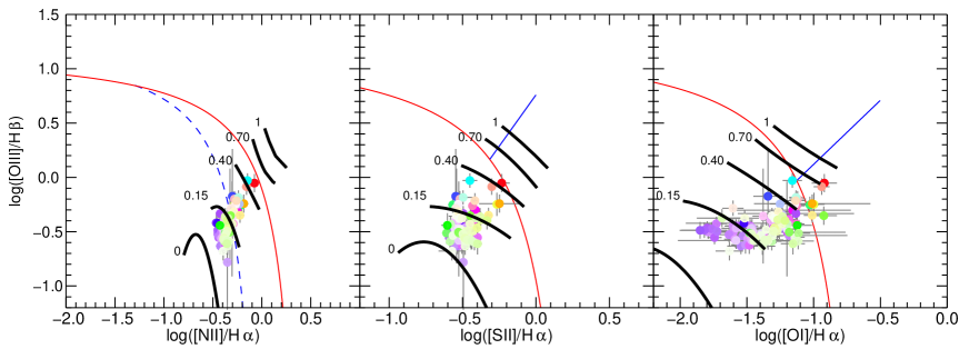
Figure 12: Line flux diagnostic diagrams of the different regions of SOS 114372 (see text). The shock and photoionization models by Rich et al. (2011) are superimposed on the measured flux ratios. The black curves are drawn for different fractions (from 0 to 1) of H$\alpha$ flux contributed by shocks as indicated. For comparison the theoretical (red curve) and empirical (blue dashed curve in the left panel) upper limits for HII regions are also indicated as well as the separation between AGN and LINER (solid blue line in the central and right panel).

In Fig. 12 we show the measured line ratios for the different galaxy regions, colour coded as in Fig. 11, along with the theoretical predictions and limits for photoionization and shock excited models. The red curves mark the theoretical upper limit for HII regions, while the dashed blue curve in the left panel delineates the empirical limit to star-forming regions defined by Kauffmann et al. (2003). Between the red curve and the dashed blue curve, ‘composite’ systems are found whose emission is characterized by a mixture of AGN and HII regions. The blue continuous line in the central and right panels divides the line ratios typical of Seyfert galaxies (upper part of the diagram), from those of low ionization emission line regions (‘LINER’). These curves are extensively used in the literature and plotted here to facilitate comparison with other works.

The black curves represent shock and photoionization models from Rich et al. (2011), in which a fraction of the radiation (as indicated by the numbers close to the curves) is produced by shock excitation and the remaining comes from photo-ionization. These models are computed using the MAPPINGS IIIr code, the latest version of the code originally introduced in Sutherland & Dopita (1993). The abundance set is taken from Grevesse et al. (2010) and we use the standard (solar region) dust depletion factors from Kimura et al. (2003). The shock models have velocities in the range 100 to 200 km s^-1 in steps of 20 km s^-1, with hydrogen assumed to be fully pre-ionized. In using these depletion factors we are implicitly assuming that the shock is not sufficiently fast to sputter the dust grains advected into the shocked region. The models presented here have Z/Z${}_{\odot}{=}2$ (log(O/H)+12$=8.99$), and have a transverse magnetic field consistent with equipartition of thermal and magnetic energy ($B{=}5$ $\mu$G for $n_{c}{=}10$ cm^-3; $B{\propto}n_{c}^{-1/2}$).

The photoionization models are generated using UV flux distributions appropriate to continuous star formation computed using the Starburst99 code (Leitherer et al., 1999). We have used the older models employed by Kewley et al. (2001) rather than more recent ones, since the hardness of the radiation field provides a closer match to the HII region line ratios observed in the SDSS galaxy sample. We have also adjusted the nitrogen abundance to provide a still closer match to the SDSS galaxies. The photoionization models are characterized by an ionization parameter $6.5{<}\log[q]{<}7.75$ cm s^-1. This ionization parameter can be converted to the more commonly used dimensionless ionization parameter $U$ by $U{=}q/c$, where $c$ is the speed of light.

We have created mixing models between each photoionization model, and all shock models. These are characterized by a fraction $f$ of the flux at H$\alpha\,$being contributed by shocks. These models do not create a simple mixing line on the diagnostic plots, but rather a zone within which the line ratios are consistent with a certain mixing fraction of shock excitation. In Fig. 12 we show the average of the line ratios produced by mixing fractions, $f{=}0$, 0.15, 0.4, 0.7 and 1.0. Note that the line ratios are sensitive to quite small contributions from shock emission - as little as 15% contribution by shocks can change observed line ratios by a factor of two.

The observed line ratios cannot be simply explained by HII-like photoionization, but display a spread which is characteristic of a mixture of both shock excitation and photoionization. All parts of the galaxy seem to be contaminated by at least a small fraction of shock excitation, $0.05{\mathrel{\hbox{\hbox to0.0pt{\hbox{\lower 4.0pt\hbox{$\sim$}}\hss}\hbox{$<$}}}}f{\mathrel{\hbox{\hbox to0.0pt{\hbox{\lower 4.0pt\hbox{$\sim$}}\hss}\hbox{$<$}}}}0.1$. The regions which are dominated by star formation and the associated HII regions are preferentially located in the SW portion of the galaxy (purple points). Regions in the extraplanar gas to the NW of the galaxy (red/orange points) have much higher shock excitation fractions, ranging up to 0.4–0.8. In addition, there is a strong concentration of shock-excited gas along the minor axis SE from the nucleus (light blue points) and in another Northern region of the SE edge (green point).

7.2 Star formation across the galaxy

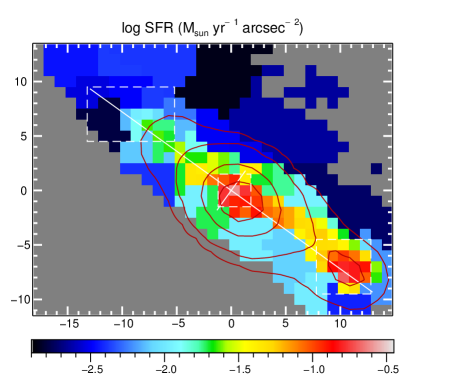
Figure 13: The logarithmic SFR density across the galaxy derived from H$\alpha$ flux corrected for the extinction and shock-excitation, where necessary. The contours show the isophotes of the 24$\mu$m flux. The three boxes outlined by white dashed sides mark the regions of the galaxy where the stellar population analysis was performed. The three regions are, from right-bottom to top-left: the starbursting region in the SW disc, the central bulge region, and the NE disc.

To study the star formation across SOS 114372, we first analyze the ongoing star formation from the flux of the H$\alpha$ emission line. Then we study the recent star formation history from the distribution of the ages of stellar populations in three distinct regions of the galaxy - a starbursting region in the SW disc (see below), the central bulge region, and the NE disc (see Fig.13).

7.2.1 Ongoing star formation

We derive the current SFR from the H$\alpha$ flux taking into account the effects of dust extinction following Kennicutt (1998). For the derivation of the SFR we approximately removed the contribution of the shock-ionized gas to the H$\alpha$ flux – the H$\alpha$ fluxes of the galaxy regions with $\geq$50% of emission coming from shock-ionized gas are reduced by a factor of two. This correction is however very small compared to the uncertainties. The logarithm of SFR surface density across the galaxy is given in Fig. 13. Intense star formation is found in the disc spanning from 0.01 to 0.34 M_⊙ yr^-1arcsec^-2 with the global maximum located in the galaxy centre. There is also a notable local maximum in the SW region of the disc at $\sim$ 12 kpc from the centre, with SFR=0.2 M_⊙ yr^-1arcsec^-2. The contours in Fig. 13 show the distribution of the 24$\mu$m flux which, in agreement with the SFR derived form H$\alpha$, presents the maximum in the centre and the second peak in the SW side. These two regions are also the most obscured regions identified in Fig. 10. These results imply a coherent scenario where the current SFR, derived from the H$\alpha$ emission and the 24$\mu$m flux, occurs in the highly dust-extinguished molecular clouds. The integrated H$\alpha$-derived SFR of SOS 114372 (adopting the Kroupa IMF) amounts to 7.2$\pm$2.2 M_⊙ yr^-1. The error takes into account the uncertainties related to the flux and attenuation measurements added to a 30% uncertainty due to different calibrations of H$\alpha$ as a SFR indicator (Kennicutt, 1998). From the difference between raw and attenuation-corrected H$\alpha$ fluxes we can estimate the obscured SFR as 5.3$\pm$1.6 M_⊙ yr^-1. This obscured SFR is also measured by the IR dust emission turning out to be 6.65${}^{+1.99}_{-1.19}$ M_⊙ yr^-1. The two independent estimates of the obscured SFR are therefore fully consistent.

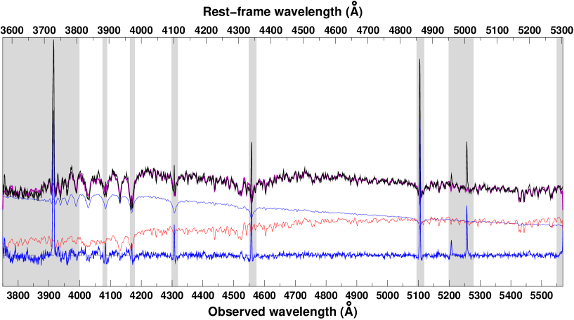
Figure 14: The integrated spectrum (black curve) and full population synthesis fit (magenta) for the starburst region in the SW side of the disc. The contributions to the model fit from the old (${>}1$ Gyr; thin red curve) and young (${\leq}1$ Gyr; thin blue) stellar populations are shown. The shaded regions indicate the wavelength ranges excluded from the fitting process. The residual emission component after subtraction of the model stellar continuum is shown by the thick blue curve.

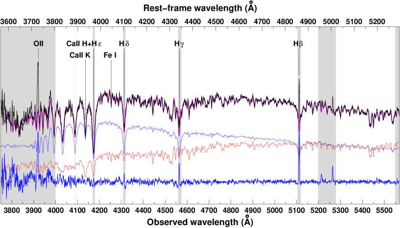
Figure 15: The integrated spectrum (black curve) and full population synthesis fit (magenta) for the NE side of the disc. The curves are coloured as in Fig 14. The line indices discussed in the text are indicated.

7.2.2 Recent star formation history

Having seen that the distribution of dust obscuration and ongoing star formation is strongly asymmetric, being significantly reduced in the NE side of the disc, while the SW side shows an ongoing highly obscured starburst, we now examine the three regions of the galaxy indicated in Fig. 13 (SW disk starburst, central bulge starburst, NE disk) separately. To determine the ages of stellar populations, we fit the spectrum with a non-negative linear combination of 40 SSPs, this time with attenuation of the stellar component by dust also left as a single free parameter (we do not consider selective attenuation for the youngest stellar populations), resulting in the best-fit model for the stellar spectrum. This is then subtracted, leaving the residual noise and emission spectrum. To achieve the signal-to-noise ratio needed for this analysis, we added the spectra within each of the three regions indicated in Fig.13.

In the SW disc starburst region (Fig. 14), the shape of the continuum, together with the weak 4000Å break ($d_{n}4000{=}1.09$), indicate that the spectrum is dominated by young stars. This is confirmed if we split our best-fit model into its contribution from young (${\leq}1$ Gyr; thin blue curve) and old (${>}1$ Gyr; thin red curve) stars. Young stars contribute $\sim$60% of the blue luminosity and ${\sim}3$.5% of the stellar mass in this region. Of this young (${\leq}1$ Gyr) component, 35% of the stellar mass and 60% of the luminosity comes from stars younger than ${\sim}1$00 Myr. This implies a starburst characterised by a $\sim 5\times$ increase in the SFR over the last $\sim$100 Myr. This burst is ongoing as implied by the very strong (despite being highly obscured with A${}_{V}{\sim}1$.9–2.6; Fig. 10) H$\alpha$ emission in this region with EW(H$\alpha){\sim}120$Å. Further Balmer emission lines are visible in Fig. 14, from H$\beta$ all the way up to H$\zeta$. The old stellar component (red curve) can be simply characterized as a single 10-15 Gyr old population.

In the central bulge region (see Fig. 2), the shape of the continuum appears dominated by an old stellar population. The splitting of our model stellar populations into old and young, shows that young stars contribute just ${\sim}3$0% of the luminosity and 1.0% of the stellar mass. Moreover, young stars are predominately of age ${\mathrel{\hbox{\hbox to0.0pt{\hbox{\lower 4.0pt\hbox{$\sim$}}\hss}\hbox{$<$}}}}100$ Myr, as also suggested by the overall smooth appearance of the continuum from this component.

In the NE disc region (Fig. 15), the stellar continuum is dominated by young (${\leq}1$ Gyr) stars, contributing to $\sim$60% of the luminosity and ${\sim}4$% of the total stellar mass. Our stellar population modeling of the young component suggests multiple populations spread over the full range 60–1000 Myr with just ${\sim}5$% of the stellar mass in this young component coming from stars younger than 100 Myr. This suggests that the average SFR over the last ${\sim}10$0 Myr is ${\sim}2{\times}$ lower than that averaged over the last Gyr.

To better understand this situation, we compare the stregths of [Oii] and H$\beta$ emission lines, which trace the ongoing star formation, to the H$\delta$ absorption line, tracing the intermediate-age ($\sim$1 Gyr) A-type stars. We measure EW([Oii])=-5.2$\pm$0.06Å,
EW(H$\delta){=}5.24{\pm}0.$08Å and EW(H$\beta$)=-2.19$\pm$0.06Å.
This combination of line strenghts places the NE disc on the boundary between the weak post-starburst (k+a) and e(a) (post-starbust with residual star-formation) classes
(see Dressler et al., 1999). The mean relation between EW(H$\delta$) and EW([Oii]) derived by Dressler et al. (2004) for normal star-forming galaxies predicts an EW(H$\delta$)$\sim$2.0 Å for a galaxy with EW([Oii])=-5 Å. The fact that our observed level of H$\delta$ absorption is somewhat higher than expected again indicates that the current SFR is significantly lower than that averaged over the previous Gyr.

As a further probe of the ongoing-to-recent SFRs we derived the Rose Caii index (Rose, 1985), which is defined as the ratio of the counts in the bottoms of the Caii H+H$\epsilon$ and Caii K lines. Rose (1985) showed that the Caii index is constant at ${\sim}1.2$ for stars later than about F2, but decreases to a minimum of ${\sim}0.4$ for A0 stars as the Caii lines weaken, before increasing again as the H${\epsilon}$ line fades. Furthermore, Leonardi & Rose (1996) combined the Caii index to the H$\delta$/Fe i $\lambda$4045 index to determine both the duration and the strength of starbursts. We measure a Caii index of 0.635 and a H$\delta$/Fe i $\lambda$4045 index of 0.745. These values confirm that our spectrum is dominated by A-type stars and, more importantly, show that we are observing a starburst which lasted for $\sim$0.3 Gyr and which has been just shut down (cf. Fig. 4 of Leonardi & Rose, 1996).

In summary, the total SFR from the H$\alpha$ flux amounts to 7.2$\pm$2.2 M_⊙ yr^-1 fully consistent with the previous estimates from UV and FIR measurements. The star formation across the galaxy mainly takes place in two regions - in the central bulge region and $\sim$ 12 kpc SW from the centre. In the central bulge region there is an intense ongoing, heavily obscured star formation accounting for $\sim$30% of the total SFR of SOS 114372. In the SW starbursting region, which accounts for $\sim$20% of the total SFR, our data imply a starburst characterised by a $5{\times}$ increase in the SFR over the last ${\sim}10$0 Myr. This burst is ongoing. In the NE disc, our data still show ongoing star formation, but significantly lower than in the rest of the disc. The full spectral modeling and the line strengths show that we are observing a 0.3 Gyr starburst immediately after it has been shut down.

8 Origin of the extraplanar gas

The most prominent and notable physical characteristic of SOS 114372 is the extraplanar ionized gas extending out to a projected distance of 13 kpc NW from the disc over its full extent following the rotation of the disc. This gas is resolved into a complex of compact H$\alpha$-emitting knots and faint filamentary structures and shows a high fraction (0.4-0.8) of shock excitation. All this supports a scenario in which gas is being driven out from the galaxy disc. The high levels of dust attenuation with $A_{V}{\sim}1$.9 mag also found associated with the extraplanar gas, suggests that the dust is stripped and dragged away from the disc together with gas, in agreement with the reduced dust disc observed in HI-deficient Virgo galaxies by Cortese et al. (2010).

Causes of large-scale outflows of gas from a galactic disc may be galactic winds produced by AGN or starbursts, tidal interaction or ram-pressure stripping. In the following we will outline the arguments that lead to the idea that RPS is actually the origin of the observed gas outflow.

8.1 Galactic winds

We notice that the outflow takes place almost uniformly all over the disc and is observed only in one direction (NW, see Figs. 5 and 6). Since it extends in projection several kiloparsecs outside of the disc, dust attenuation could not hide a possible (symmetric) component on the SE side. The observed outflow is therefore intrinsically asymmetric. Galactic winds, instead, produce bipolar outflows, with a structure ranging from biconical to egg-shaped, originating from a nuclear starburst or AGN, and extending on both sides of the disc (Veilleux et al., 2005, and references therein). We therefore exclude a galactic wind as the cause of the bulk of the gas outflow observed here.

Nevertheless, we don’t exclude that a galactic wind could actually be in place close to the nucleus, where star formation is taking place at a rate of $\sim$2 M_⊙yr^-1 and the H$\alpha$ image shows hints of gas escaping from the centre of the SE disc (see Fig. 6). Let us consider the area with very high values of the velocity dispersion (${\mathrel{\hbox{\hbox to0.0pt{\hbox{\lower 4.0pt\hbox{$\sim$}}\hss}\hbox{$>$}}}}$ 120 km s^-1, Fig. 7) located along the minor axis SE from the galaxy centre. We notice that this area has a roughly triangular shape, with a vertex near the galaxy centre. The minor axis radial velocity profile (Fig. 8) shows that the gas is moving towards the observer, with a speed steadily rising up to $\sim$100 km s^-1 at $\sim 3$ kpc from the centre. The high values of $\sigma$ suggest the presence of different components of gas with different radial velocities, so that the measured $\sim$100 km s^-1 is an average velocity (weighted by the H_α flux).

All these features, together with the fact that the radiation here is shock-dominated (Sect. 7.1), suggests that the triangular region SE from the centre may be a semi-cone produced by the nuclear starburst (Veilleux et al., 2005). The absence of the companion semi-cone in the NW direction could be explained by dust absorption if the disc is oriented with the SE side furthest from us. We will add further support for this orientation in Sect. 9. Given the inclination of the galaxy and the apparent extension of the wind cone of 6.5 arcsec from the centre, and allowing for large uncertainties due to poor spatial resolution, we infer that the cone extends $\sim$ 6 kpc above the disc, within the typical sizes of observed galactic winds (Veilleux et al., 2005).

As already noted, the area SE from the nucleus is the most dust-obscured (excluding the nuclear region itself; Fig. 10). This would be easily explained by a large amount of dust collected in the starbursting region and entrained in the wind, which is a rather common circumstance in galactic winds (Hoopes et al., 2005, and references therein).

8.2 Tidal interaction

The best candidates for a major tidal interaction are the cluster members SOS 114493 and SOS 112392 (Fig. 1 and  16) with redshifts $z=0.050$ and $z=0.046$ and $K$-band magnitudes 13.49 mag and 12.61 mag, respectively. These two galaxies are at projected distance from SOS 114372 of $\sim$45 kpc and $\sim$55 kpc respectively, and their stellar masses are $\mathcal{M}_{114493}$=$2{\cdot}10^{10}$M_⊙ and $\mathcal{M}_{112392}$=$7{\cdot}10^{10}$M_⊙ (Paper I). We observe no tidal bridge connecting SOS 114372 to either of these objects nor any signs of disturbance in their $R$-band images, as is shown in Fig. 16. The direction of the gas outflow from SOS 114372 does not appear to be related to any of these galaxies. Furthermore, no obvious sign of perturbation is present in any of SSC galaxies within 200 kpc projected radius from SOS 114372.

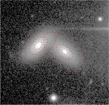
Figure 16: Close-up of SOS 114493 (left) and SOS 112392 (right) from a ESO-2.2m WFI deep R-band image. The intensities are stretched by a logarithmic scaling to emphasize the lowest surface brightness regions. The deep-red ellipses are drawn from the models derived from a simultaneous fit to the two galaxies using two Sérsic laws. The fit was performed with GALFIT (Peng et al., 2010). The surface brightness of both galaxies smoothly follow the models without any appreciable sign of perturbation. One side of this figure corresponds to $\sim$45 kpc.

As already noted in Sect. 6.2, the stellar velocity field of SOS 114372 displays no sign of disturbances, indicating that the galaxy is not suffering any significant external gravitational perturbation. The lack of a tidal tail, the undisturbed stellar disc, the existence itself of the gas disc, and the absence of perturbed neighbours make us exclude the occurrence of tidal interaction, unless it is at a very early stage, with the closer galaxy (at a distance anyway $>$ 45 kpc) just starting its first approach. Numerical simulations (Kronberger et al., 2006, 2007), however, do not predict gas outflow at this stage, either for two galaxies of the same mass (as in the case of SOS 114372–SOS 112392) or for the unequal-mass case (as for SOS 114372–SOS 114493).

The next candidate for a tidal interaction is the faint object located SW of SOS 114372 (SOS 115228, see Fig. 1 right panel). Although we do not have redshift information for this galaxy, it appears much brighter in our narrow-band H$\alpha$ image than in the continuum, which would suggest that it is a starbursting dwarf galaxy at a redshift within a few hundred km s^-1 of SOS 114372. As tidal torques are effective in channelling rapid gas inflows capable of fuelling nuclear starbursts, it seems reasonable that an interaction between SOS 114372 and SOS 115228 could be behind the observed starburst in the dwarf galaxy. It is much less likely that this interaction could induce the large-scale gas outflow in SOS 114372 however. Firstly, the $K$-band magnitudes of the two galaxies differ by $\sim$ 5 mag, and we found a factor about 360 difference in stellar masses (Paper I). This makes it unlikely that this object can have such a large-scale effect on the gas of its much more massive neighbour. Secondly, simulations of unequal mass mergers predict gas streams connecting the two galaxies (see Fig. 6 of Kronberger et al. 2006), while we observe the gas outflow in the opposite direction. We find no evidence at all for a tidal bridge connecting the two galaxies, although Kapferer et al. (2009a) find that in clusters the impact of pressure from the ambient ICM can destroy these tidal bridges, as well as further enhance the levels of star formation in the interacting galaxies. Notice, however, that the simulated galaxies considered by Kronberger et al. (2006) to investigate the unequal mass merger have at most a mass ratio equal to 8:1. It may be that the notable starburst on the SW-edge of SOS 114372 is caused by such a combination of the tidal interaction and ram pressure stripping. Finally, as already noted in Sect. 6.1, it is possible that SOS 115228 is at a completely different redshift from SOS 114372.

All the above considerations and most importantly the symmetric stellar distribution of the three brighter galaxies lead us to conclude that tidal interaction is not the cause of the observed gas outflow.

8.3 Ram-pressure stripping

The large-scale gas outflow detected by the IFS data is resolved in the narrow-band H$\alpha$ imaging into a complex of compact knots of H$\alpha$ emission, often attached to faint filamentary strands which extend back to the galactic disc (Fig. 6). Similar complexes of H$\alpha$ or UV-emitting knots and filaments have been seen for numerous other galaxies (e.g. Gavazzi et al., 2001; Cortese et al., 2007; Yagi et al., 2010; Vollmer et al., 2010; Fossati et al., 2012). The most notable aspects of these systems are that all the affected galaxies are located in cluster environments, and that the outflow is one-sided, often characterized as a cometary tail of ionized gas directed away from the cluster centre. These two aspects both point to a cluster-specific process in which gas is stripped from an infalling galaxy by its passage through the ICM.

The H$\alpha$ velocity field of SOS 114372 can be compared with those of nearby galaxies affected by RPS such as NGC 4438 (Chemin et al., 2005; Vollmer et al., 2009) and NGC 4522 (Vollmer et al., 2000) in the Virgo cluster. Both galaxies show one-sided extraplanar gas following the rotation of the disc, as for SOS 114372. The velocity field of NGC 4438 is characterized by filamentary structures extending out of the disc. If present, such filaments could not be resolved at the higher redshift of SOS 114372 with our IFS data. Remarkable analogies are found in the H$\alpha$ images of the two galaxies (compare Fig. 2 of Kenney & Koopmann 1999 with our Fig. 6). Kenney & Koopmann (1999) observed that the H$\alpha$ emission arising from both HII  regions and diffuse emission is organized in filaments extending more than 3 kpc from the outer edge. The difference between the two galaxies is in the truncation radius - NGC 4522 has a truncated gas disc at radius of 3 kpc, while in the case of SOS 114372 the ionized gas extends up to 13 kpc. This difference can be related to different ’ages’ of RPS, different orbits, ICM densities and ICM wind angles. We also notice that there are intrinsic differences between the two Virgo galaxies and that studied in this article. SOS 114372 has an absolute $B$-band magnitude of M${}_{B}=-21.48$, significantly brighter than M${}_{B}=-20.04$ and M${}_{B}=-18.10$ of NGC 4438 and NGC 4522, respectively (assuming 16 Mpc as distance of the Virgo cluster and the magnitudes from Chung et al. 2009). This shows that we are comparing galaxies of different masses. Furthermore, NGC 4438 is located close to the Virgo cluster centre (280 kpc from M87, $r\sim$0.3$r_{200}$) while NGC 4522 is at $r\sim r_{200}$ (Urban e al., 2011) and SOS 114372 is at $r\sim$1 Mpc ($\sim$0.5$r_{200}$) from the centre of the rich cluster A 3558. It is therefore likely that these galaxies are experiencing different ICM-ISM interactions. The common point between the velocity fields of NGC 4522, NGC 4438, and SOS 114372 is that the extraplanar regions are still dominated by rotation.

Hydrodynamical simulations show that ram-pressure and viscous stripping of spiral galaxies produce narrow wakes of Hi gas that can extend up to 100–200 kpc and last 500 Myr (Tonnesen & Bryan, 2010). These simulations predict a wide range of densities and temperatures within these tails, leading to the in-situ formation of pressure-supported clouds dense enough to form stars. This star-formation plus localized heating via compression and turbulence can light up the Hi tail with H$\alpha$ emission, with intensities and morphologies (Tonnesen & Bryan, 2012) similar to those observed in SOS 114372. Tonnesen & Bryan (2012) note that this star formation in the tail does not occur due to molecular clouds that were formed within the galaxy itself and stripped wholesale, but rather because the relatively low-density gas that has been stripped can cool and condense into dense clouds in the turbulent wake. They also indicate that higher ICM pressures create more dense clouds in the wakes, resulting in higher SFRs.

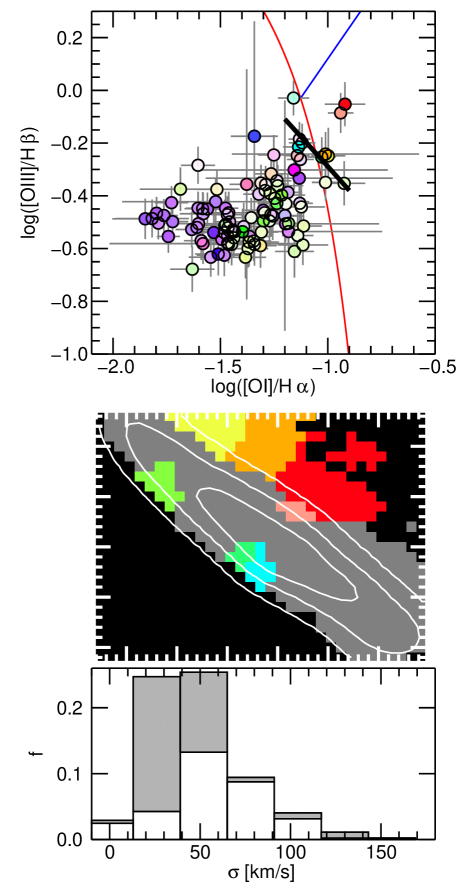
Figure 17: Upper panel: The flux ratios in the different galaxy regions as in Fig. 12. The black curve corresponds to the shock and photoionization model where 50% of the flux is due to shock-ionized gas. Central panel: The galaxy regions dominated by the contribution of shock-ionized gas colour-coded as in Fig. 17. Lower panel: Normalized distribution of the velocity dispersion values. The white coloured histogram refers to the regions dominated by the contribution of shock-ionized gas, while the gray histogram refers to the “low” shock-ionized gas region. The regions characterized by shock-like line ratios tend to have higher velocity dispersions.

Nevertheless, star formation cannot be the only origin of the H$\alpha$ emission coming from the outflowing gas. In Fig. 17 (upper panel) we focus again on the right panel of Fig 12, which plots the [Oiii]/H$\beta$ versus [Oi]/H$\alpha$ diagnostic. There are seven galaxy regions where shock excitation contributes more than 50% of the emission. Their flux ratios are located to the right side of the black curve in upper panel of Fig. 17 and are coloured in the central panel. These regions correspond to the gas outflow and to three regions in the SE edge of the galaxy. In all these regions, except the easternmost one (shown in light green), we also measure strong dust extinction. The normalized distribution of the velocity dispersion measured for these regions (white coloured histogram in Fig. 17) is shifted to higher values with respect to the overall distribution. We expect the velocity dispersion produced by the shocks to be of the same order as the shock velocity. If $n_{ICM}$ and $n_{ISM}$ are the number densities of the ICM and ISM respectively and if $v_{o}$ is the relative velocity of the two gas components, then the shock velocity is $v_{s}$=$\sqrt{(}n_{ICM}/n_{ISM})\times v_{o}$. If $n_{ICM}/n_{ISM}\sim$ 10^-2–10^-3 and $v_{o}\sim$ 1000  km  s^-1 then $v_{s}\sim$30-100 km  s^-1, which is what we observe. The high velocity dispersions of some non-shocked regions may be well explained by the complicated radial motions produced by ram pressure and by the fact that our resolution element intercepts gas clouds for depths of $\mathrel{\hbox{\hbox to0.0pt{\hbox{\lower 4.0pt\hbox{$\sim$}}\hss}\hbox{$>$}}}1/cos\ i\sim$ 7 kpc.

From the distribution of the regions with higher velocity dispersion and shock-ionized gas across the galaxy, we can infer that SOS 114372 is affected by ram pressure which compresses and strips the gas out of the galaxy, forming a tail of turbulent shock-ionized gas and dust. Part of this gas can cool and condense into dense clouds observed in H$\alpha$.

The influence of RPS on the internal kinematics has been investigated through N-body/hydrodynamical simulations by Kronberger et al. (2008b) demonstrating that the gas velocity field shows clear evidence of disturbances after a few tens of Myr from the onset of RPS. In particular, the rotation curve can be characterized by asymmetry in the external gas disc while the inner disc remains undisturbed. A measure of the disturbance is given by the asymmetry parameter of the rotation curve as defined by Dale et al. (2001). We estimate an asymmetry parameter of about 20% for the SOS 114372 major axis radial velocity profile, consistent with what estimated by Kronberger et al. (2008b) for RPS. Moreover the major axis velocity profile of SOS 144372 (extending to ${\sim}3.8{\times}r_{d}$; Fig. 8) is very similar to the gas rotation curve derived for the model galaxies after 50 Myr of ram pressure acting face-on (Fig. 2 of Kronberger et al. 2008b) extending to $4{\times}r_{d}$.

SOS 114372 is amongst the brightest SSC galaxies in the mid-infrared with one of the highest SFRs measured for the whole sample (see Paper II). The galaxy centre and the SW region of the disc contribute $\sim$30% and $\sim$20% respectively to the total SFR measured by the H$\alpha$ luminosity (i.e. current SFR). The location of the star-forming regions in the galaxy agrees with the predictions of the simulations of RPS where the newly formed stars are preferentially located in the compressed central region of the galaxy and/or in the stripped gas behind the galaxy (Kronberger et al., 2008a) depending on the surrounding gas density (Kapferer et al., 2009b). Sanderson & Ponman (2010) estimated an ICM density of $\rho_{ICM}=1.3\times 10^{-28}$g cm^-3 at the projected distance of the galaxy from the cluster core. This density implies that all the newly formed stars are confined into the disc either because of the low ICM density or because the RPS has started less than 100 Myr ago (Kapferer et al., 2009b). The starburst detected in the SW disc region produces a ${\sim}5{\times}$ increase in the SFR over the last ${\sim}10^{8}$ yr and could be ram-pressure induced. Also in the central bulge region, whose spectrum is clearly dominated by old (${>}1$ Gyr) stars, we measure a non-negligible contribution from young (${\mathrel{\hbox{\hbox to0.0pt{\hbox{\lower 4.0pt\hbox{$\sim$}}\hss}\hbox{$<$}}}}10^{8}$ yr) stars, but this star-forming region is most probably related to the presence of the bar (see Sect. 10).

The asymmetry observed in the SFR and stellar population properties across the galaxy disc can be explained in a RPS scenario where the ram pressure contributes to the star formation quenching via the impoverishment of the gas reservoir, while inducing the ongoing starburst in the highly obscured SW side. Different stripping efficiencies depending on the surface density of the stripped gas clumps are also found by Vollmer et al. (2009).

We can thus conclude that all the observed properties of SOS 114372 can be accommodated in the RPS scenario.

8.4 Environmental conditions for
ram-pressure stripping

Now we consider the ICM properties in order to check if RPS can be effective for this galaxy.

For A 3558, Sanderson & Ponman (2010) derived the dark matter density, gas density ($\rho_{ICM}$) and the gas temperature profiles by fitting Ascasibar & Diego (2008) models to the Chandra X-ray data. In these models, the dark matter is described by a Hernquist (1990) density profile, which provides simple analytic expressions for the mass profile, gravitational potential and escape velocity. From this, we can derive the ram pressure, $P_{ram}{=}\rho_{ICM}v_{orb}^{2}$, acting on galaxies as function of cluster-centric radius and orbital velocity (Haines et al. 2011c). For the cluster-centric radius we assume the projected distance of 0.995 Mpc. As a lower limit for the orbital velocity, we assume the galaxy’s line-of-sight velocity relative to the cluster’s systemic velocity $V_{los}\sim$830 km s^-1, For the upper limit we assume the escape velocity at the cluster-centric distance which, from the Henrquist model for A 3558, is $\sim$2600 km s^-1. At 0.995 Mpc from the cluster centre $\rho_{ICM}\simeq$1.3$\cdot$10^-28 g cm^-3 and the ram pressure ranges from $\sim$9$\cdot$10^-13 dyn cm^-2 to $\sim$9$\cdot$10^-12 dyn cm^-2. This is the regime of weak to moderate ram pressure as defined by Roediger & Hensler (2005) who, by means of high resolution 2D hydrodynamical simulations, demonstrated that ram pressure effects can be observed over a wide range of ICM conditions. In particular, in high density environments RPS severely truncates the gas disc of $L^{\star}$ galaxies, while in low density environments, where moderate ram pressure is foreseen, their gas disc is clearly disturbed and bent (Roediger & Hensler, 2005) as we observe. The gas discs of these galaxies can be truncated to 15-20 kpc in the first 20–200 Myr of RPS. To check if the expected ram pressure is able to strip the gas from the disc of SOS 114372, we estimate the gravitational restoring force per unit area $(d\phi/dz)\sigma_{gas}=2\pi G\sigma_{disc}\sigma_{gas}$, with $\sigma_{star}$ and $\sigma_{disc}$ the star and gas surface density, respectively. From the $K$-band photometry, we derive the inclination- and dust attenuation-corrected surface brightness at 20 kpc (where the gas disc is bent) of 4.4 L_⊙pc^-2. From the $K$-band luminosity and the stellar mass (see Table 1), we obtain M/L${}_{K}\sim$2, therefore the stellar mass surface density is 8.8 M_⊙pc^-2. Assuming a typical $\sigma_{gas}\sim 10$ M_⊙pc^-2, the restoring force per unit area is $1.7\cdot 10^{-12}$ dyn cm^-2 which compared with the estimated ram pressure (9$\cdot$10^-13–9$\cdot$10^-12 dyn cm^-2) shows that it can be effective in removing the gas from the disk if $v_{orb}\geq 1100$ km s^-1. We assume that the galaxy is coming in radially, such that the projected cluster-centric distance is the same as the actual 3D one. If the galaxy is at a larger 3D distance, then the local density will be lower, as will the wind velocity, and thus the ram pressure could be overestimated although a moving ICM and/or local overdensities can enhance it.

Crowl & Kenney (2006, 2008) conducted a survey of ten Virgo galaxies with the SparsePak IFS. They found clear evidence of RPS-induced star formation within the truncation radius and a passive population beyond it. Their estimates of the stripping timescales showed that Virgo galaxies can be stripped both within and beyond the cluster core. This is direct evidence that the ICM is neither static nor homogeneous. That a galaxy’s ISM can be affected by the environment also in intermediate- to low-density regions (0.6–1.0 Mpc from the cluster cD galaxy) in the Virgo cluster was also concluded by Chung et al. (2007) observing the HI tails of seven spiral galaxies.

A non homogeneous ICM is expected for non virialized merging and post-merging clusters. Dynamical analyses (Bardelli at al., 1998) and X-ray observations (Bardelli et al. 1996; Akimoto et al. 2003) of A 3558 indicate this cluster is the result of a cluster-cluster merging and/or a group infall. More recently, combining XMM-Newton and $Chandra$ data, Rossetti et al. (2007) were able to detect a cold front in the A 3558 ICM probably caused by the sloshing of the core induced by the perturbation of the gravitational potential associated with a past merger. This cold front is expanding, perturbing the density and the temperature of the ICM. From their Fig. 3 it is clear that the cold front is moving in the direction of SOS 114372 and that it is $\sim$5 arcmin ($\sim 300$ kpc in projection) from the galaxy. Unfortunately, the X-ray observations do not include the region of SOS 114372, which is planned to be observed in future surveys (see Hudaveri, Bozkurt & Ercan 2010).

Taking into account all the above arguments, we conclude that the environment of our galaxy is favourable to RPS despite its large distance from the cluster centre.

9 N-body/hydrodynamical simulations of ram-pressure stripping

To confirm the scenario of RPS and to constrain its physics, we performed N-body/hydrodynamical simulations. Our aim was to reproduce as closely as possible the velocity field of the gas. We remark that in the real system there are factors that cannot be accounted for in a simulation, such as the spatial distribution of the dust, which may affect the observed kinematics and distribution of the gas. The interaction of the ICM with the ISM may also be complicated by their clumpiness, not to mention the action of the bar. We therefore don’t expect the simulations to provide a description of the details of the gas kinematics, but aim to obtain an overall agreement with the observations helping us to constrain the ICM wind angle and velocity and the ‘age’ of RPS.

Table 2: The model galaxy. Properties of the initial conditions of the model galaxy used. The particle numbers, mass resolution and cumulative mass are shown for disc scale length corresponding to 10% of the disc radius both for low- and high-resolution simulations (LR, HR).

	# of particles	mass resolution	total mass
		$\left[M_{\odot}/particle\right]$	$\left[M_{\odot}\right]$
HR
DM halo	$3\times 10^{5}$	$3.7\times 10^{6}$	$1.1\times 10^{12}$
gas disc	$2\times 10^{5}$	$2.9\times 10^{4}$	$5.9\times 10^{9}$
stellar disc	$2\times 10^{5}$	$2.6\times 10^{5}$	$5.3\times 10^{10}$
stellar bulge	$1\times 10^{5}$	$1.7\times 10^{5}$	$1.7\times 10^{10}$
LR
DM halo	$3\times 10^{4}$	$3.7\times 10^{7}$	$1.1\times 10^{12}$
gas disc	$2\times 10^{4}$	$2.9\times 10^{5}$	$5.9\times 10^{9}$
stellar disc	$2\times 10^{4}$	$2.6\times 10^{6}$	$5.3\times 10^{10}$
stellar bulge	$1\times 10^{4}$	$1.7\times 10^{6}$	$1.7\times 10^{10}$

9.1 Simulations

An important aspect of the use of simulations is that, at least in the early phases of RPS, the direction of the ICM wind cannot be inferred from the apparent direction of the gas outflow, because the motion of the gas is a complex combination of the effects of the ram pressure and the gravitational field of the host galaxy (see also Roedigger & Brüggen 2006). Clarke et al. (1998) introduced a geometrical scheme (see their Fig. 1) to study the jets in Seyfert galaxies. In that scheme, the angle between the jet and the normal to the disc is constrained by the apparent jet outflow angle and the inclination of the galaxy. In a different framework, that scheme was adopted by Abramson et al. (2011) to study the geometry of RPS, substituting the jet direction with the ICM wind direction.

Unfortunately, we cannot adopt Clarke et al.’s scheme for two reasons. The first reason is that the rotation of the galaxy breaks one important symmetry that lies at the ground of the applicability of that scheme. The second reason is that not only the direction of the outflow does not indicate the direction of the wind, but also the direction of the wind with respect to the disc cannot be assumed a priori (see Appendix A). We therefore considered all the possible values for the angle $\beta$ between the galaxy rotation axis and the ICM wind. We ran simulations from RPS close to edge-on ($\beta=85^{\circ}$) to close to face-on ($\beta=15^{\circ}$) at intervals of 10^∘ (there was no need to explore values closer to face-on or to edge-on). For what concerns the ICM wind velocity, we set as the lower limit the galaxy’s line-of-sight velocity relative to the cluster’s systemic velocity, $V_{los}\sim$830 km s^-1, and as the upper limit the escape velocity, $\sim$2600 km s^-1 (derived from the Hernquist model for A 3558).

We explored the following values for the ICM wind velocity ($V_{wind}$=830, 1100, 1400, 1700, 2000, 2200, 2400, 2600 km s^-1). We also explored two different disc scale heights corresponding to 10% and 20% of the radius $r_{d}$. In summary, our grid of models includes 8 values for $\beta$, 8 values for $V_{wind}$ and 2 values for the disc scale height. Our approach was to run low-resolution simulations for the whole range of parameters and then select the most promising cases for the high-resolution simulations.

The simulations were done with the cosmological N-body/hydrodynamic code GADGET-2 developed by Volker Springel (Springel, 2005). The hydrodynamic part follows an SPH scheme (Gingold & Monaghan, 1977; Lucy, 1977) while the gravitational interaction is calculated using a tree code for the short range force as first introduced by Barnes & Hut (1986) and treePM code based on Fourier techniques for the long range forces. Furthermore, our version of GADGET-2 includes radiative cooling (Katz et al., 1996) and recipes for star formation, stellar feedback and galactic winds according to Springel & Hernquist (2003).

To simulate galaxies undergoing RPS, we use the same simulation setup as Kapferer et al. (2009b), Kronberger et al. (2008a) and Steinhauser et al. (2012). First, we generate a model galaxy matching the observed properties of SOS 114372 (see Sect. 2). The initial conditions are calculated according to Springel et al. (2005) based on the work of Mo et al. (1998). Our model galaxy includes a dark matter halo, a stellar disc, a gaseous disc and a stellar bulge. The disc scale length of the galaxy is directly related to the angular momentum of the disc with the spin as a free parameter. The stellar and gaseous disc have exponential surface density profiles. For the stellar bulge and the dark matter halo a Hernquist (1990) profile is adopted. Important parameters and properties adopted for our model galaxy are shown in Table 2 for both the low- and high-resolution simulations. The total mass is $\mathcal{M}_{tot}{=}1.2{\cdot}10^{12}$M_⊙ and the total (dynamical) and baryonic mass within 20 kpc are $\mathcal{M}_{dyn}{=}2.1{\cdot}10^{11}$M_⊙ (see Sect. 6.2) and $\mathcal{M}_{\star}{=}7.0{\cdot}10^{10}$M_⊙, respectively. Since the initial gas mass of SOS 114372 is not known, we assume that the gaseous phase contains 10% of the mass of the disc. The initial disc scale height was set to either 10% or 20% of the disc scale length. The disc-to-bulge mass ratio of 0.32 adopted for the model galaxy was derived from the measured B/D flux ratio of 0.44 taking into account that $\sim$30% of the light from the bulge is due to very young stars contributing only 1% to its mass (Sect. 7.2).

Since the model galaxy needs some time to settle to avoid numerical artefacts, it is evolved in isolation for 1 Gyr before the ICM wind is applied. Furthermore, the parameters for generating the model galaxy were chosen carefully to obtain a stable galaxy. As also found by Moster et al. (2011), the resolution plays an important role. As we found in the low-resolution runs in which the galaxy consists of a significantly smaller number of particles than the nominal $7.5\times 10^{5}$ value, both the stellar and the gaseous disc were puffed up, leading even to warps although the galaxy is evolving in isolation. With the chosen parameters the effect of the resolution was less dramatic and negligible on the morphology of the stripped gas, used for the selection of the models which better reproduce the observations.

To simulate the prevailing environment of
SOS 114372, the model galaxy is then exposed to an external wind, simulating the ICM. At variance with many other RPS simulations, the model galaxy itself is moving and the ICM is stationary. The gas particles representing the ICM fill a simulation domain with periodic boundary conditions in order to keep the ICM density stable during the simulation. The mass resolution of the ICM particles is the same as for the ISM particles to avoid numerical artefacts. As we use a box size of 850 kpc, a large number of particles would be needed leading to a very long computation time. For this reason, only the inner part of the cube with size $200\times 200\times 850\,\mathrm{kpc}^{3}$, where the galaxy flies through, has the same mass resolution as the ISM. On the outside, particles with a hundred times higher mass are used. For an ICM density of $\rho_{\mathrm{ICM}}=1.3\times 10^{-28}\,\mathrm{g}\,\mathrm{cm}^{-3}$ (Sanderson & Ponman, 2010), 3.1 million gas particles are needed.

The models were run from the onset of the ram pressure to 100 Myr after. During this time the ram pressure is kept constant and its onset is immediate.

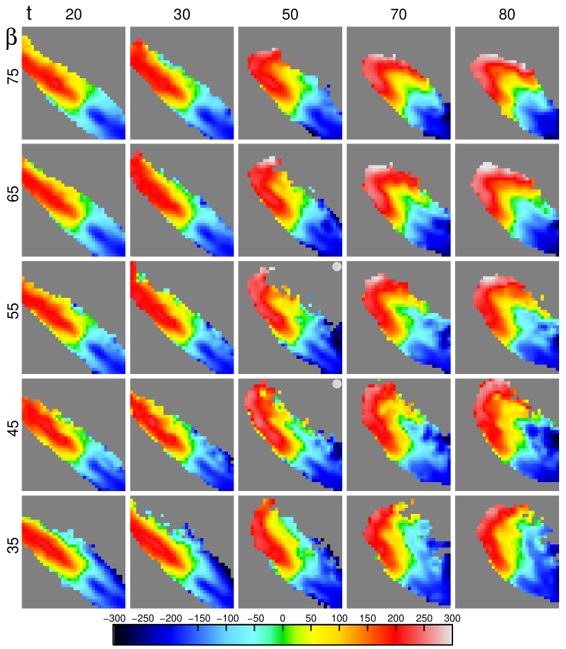
Figure 18: Example of a grid of low-resolution models. The wind angle $\beta$ (in degrees) changes in the vertical direction and the time since the onset of RPS (in Myr) in the horizontal direction as indicated. The selected models are marked with a light circle in the top-right of the thumbnails. Notice that all of the models are shown for brevity only in one projection(case $B$, see Appendix). $V_{wind}$ is fixed at 1400 km s^-1. The colour bar gives the values of radial velocity in km s^-1. Notice the progressive bending of the disc with time and the progressive truncation of the upper-left disc with $\beta$.

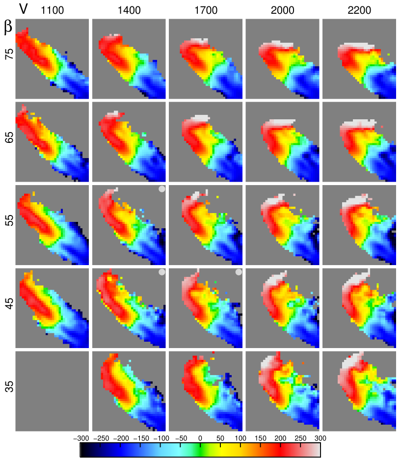
Figure 19: Analogous to Fig. 18, but with the wind velocity $V_{wind}$ in place of the time. The time is fixed at 60 Myr.

9.2 Comparison with the observations

To compare the models with the data we first accounted for the constraints on the viewing directions. The first constraint is given by the inclination angle $i$=82^∘ of the galaxy. The other constraint comes from the requirement that the spatial velocity of the galaxy $\overrightarrow{V}_{gal}$ projects into the observed $V_{los}$. This translates into the requirement that the angle $\phi$ between the motion of the galaxy and the line of sight is given by $cos\ \phi=V_{los}/V_{gal}$. As it is shown in the Appendix, the consequence of these constraints is that some models can be always observed from four directions, others from two, and others from two but only for high values of $V_{gal}$. The issue of the viewing directions is treated in detail in the Appendix where we also describe the process leading from the 3-D models provided by the simulations to the 2-D fields comparable with our data. In brief, to compare the models with the observations we account for the seeing effect associating to each particle of the simulation a Gaussian distribution with the FWHM equal to the seeing, and in each surface element of the plane of the sky we compute the surface density of particles $\Sigma$ as the sum of the contributions from the Gaussians and the radial velocity as the weighted average of the individual velocities. In the following, a case corresponding to a particular projection of a simulation (characterized by wind velocity, wind angle and time past since the onset of RPS) will be referred to as ‘case’ or ‘model’, without distinction.

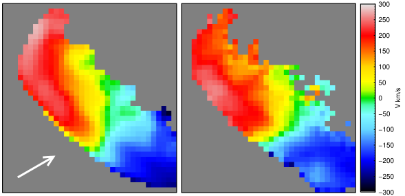
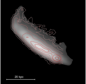
Figure 20: Left: One of the best models ( $\beta=$ 45^∘, $V_{wind}$=1400 km s^-1, t=60 Myr; left) is compared to the observed radial velocity field. The arrow shows the direction of the ICM wind. The velocity scale is to the right. Right: The contours of H$\alpha$ flux measured with WiFeS are superimposed to the gas density of the same model.

For what concerns the spatial distribution of the gas, we should keep in mind that while the simulations show the velocity field of the whole gas, our data refer to the ionized gas. However, it is reasonable to assume that the neutral and ionized gas are mixed. In their study of the ram-pressure stripped galaxy NGC 4330, Abramson et al. (2011) showed that the H$\alpha$ flux is truncated at the same radius on the SE side as the HI emission which extends slightly further in the trailing side, and Tonnesen & Bryan (2010) found that in the tail of the H$\alpha$ emission follows the neutral gas.

The first selection was made on low-resolution models. To start the selection, we compared the spatial distributions and the velocity fields of the models with the observations as explained below.

The H$\alpha$ surface brightness $F_{ij}$ was first normalized to 5$\times$10^-18erg s${-1}$cm^-2Å${-1}$arcsec^-2 so that at our 5$\sigma$ detection limit $F$=1. Then, for each case, we computed the quantity $\chi^{2}=\sum(F_{ij}-\Sigma_{ij})^{2}/(N_{pix}-1)$, where $\Sigma$ is the particle surface density of the model and $N_{pix}$ is the number of pixels where $\chi^{2}$ is evaluated. The sum was computed, in a first iteration, over the intersection between the observed area and the area where $\Sigma>$0. In this computation we masked out the two regions with very high star-formation rates, i.e. the nuclear region and the region 12 kpc SW from the nucleus. We then ranked the cases in increasing order of $\chi^{2}$ and by visual inspection verified that the ranking in $\chi^{2}$ reflects faithfully the consistency of the model gas distribution with the data.

The observed gas is confined in an area limited by our detection limit of $F$=1, while the $\Sigma$ of the models may assume arbitrarily small values. To set a lower limit to $\Sigma$ consistent with the observational limits, we derived, for each case, the mean $a$ of the ratios $\Sigma_{ij}/F_{ij}$ computed over the flux range $F$=1-10 (i.e. from our flux limit to 10$\times$ higher), and derived a mean value of $a$ averaging over the first ranked cases. We found $a$=1.21$\pm$0.23, with the low dispersion reflecting the stability of $a$ over $\sim$ 100 different models. By definition, $a$ is the particle surface density corresponding to our lowest detection value, i.e. to the “borders” of our data, and as such it was adopted as the cutoff value to compare the LR models with the observations. For the HR simulations, having 10 time higher particle density, we used a cutoff 10$\times$ higher than this ($a^{\prime}$=12.1) .

We then run a second iteration of the computation of $\chi^{2}$, where we set $\Sigma>a$ to cut the models consistently with the data. We also considered the size of the intersection between the observed area and the models, and accepted only the models which cover at least 80% of the observed area. In this way we could reject models whose spatial gas distribution is significantly different from the observed one. These are the cases when a substantial fraction of the gas is stripped from the disc, like in advanced phases of RPS (t$>$70 Myr) or in early phases (t$<$20 Myr), where the gas in the models is still confined in the disc. Only 38% cases survived this selection.

A similar ranking was applied to the velocity fields, defining $\chi^{2}=\sum(V^{m}_{ij}-V^{o}_{ij})^{2}/(N_{pix}-1)$, where $V^{m}_{ij}$ and $V^{o}_{ij}$ are the model and observed radial velocity fields respectively. In this case the ranking according to increasing values of $\chi^{2}$ is more prone to ‘mistakes’ than before, and actually the preferred cases are those at the extremes of time: t$\geq$80 Myr or t$\leq$20 Myr. The reason is that those models spatially overlap with the data only in the inner regions, where the velocity field of the gas is less perturbed. To remove the contamination from these cases, we had to exclude models with overlap less than 90%, which left only 5% of them. Also in the case of velocity fields we verified by visual inspection that the ranking reflects the consistency between data and models. The cases that survived this selection were further inspected visually to look for manifest inconsistencies between models and data.

Figures 18 and 19 show some models in two parameter grids ($\beta$,t and $\beta$,$V_{wind}$ respectively). Some selected models are marked with a circle on the upper-left corner of the thumbnails. From the low-resolution simulations, we selected the models with $\beta$=$45^{\circ}$ and $\beta$=$55^{\circ}$ with $V_{wind}$=1400 km s^-1 and 1700 km s^-1, and disc scale height 10% of the scale length, and carried out high-resolution simulations with these parameters. Lower and higher velocity values at the same $\beta$ values are not able to produce the observed gas outflowing or truncate the gas disc at smaller radii than observed, respectively (see Fig. 19). At a certain velocity value, $\beta$ values closer to the edge-on RPS tends to truncate the NE galaxy side sharply respect to the observations, while $\beta$ values closer to the face-on RPS presents blueshifted gas in the NW side of the disc in contrast with what observed (see Figs. 18 and 7).

The comparison of the observed velocity field with the high-resolution simulations leads to a further restriction of the parameter space. The best final model is shown in Fig. 20 (left panel) together with the observed velocity field. The projection on the plane of the sky of the ICM wind is also shown. This model corresponds to $\beta=45^{\circ}$, $V_{wind}$=1400 km s^-1 and $t=$ 60 Myr. Figure 20 (right panel) compares the gas density of the same model to the observed H$\alpha$ flux distribution. The most external isophote corresponds to our 5$\sigma$ detection limit ($F=1$) while the density of the model is consistently cut at $\Sigma=12.1$ particles per arcsec² (see above). We notice a remarkable agreement between the model and WiFeS observations. In the southwestern part of the disc not covered by WiFeS data the model is less constrained by the H$\alpha$ imaging (cf. Fig. 6 right panel) which is slightly shallower than the IFS observations.

Our data are therefore consistent with a wind angle $\beta\sim 45^{\circ}$, such that the RPS is taking place at an angle intermediate between face-on and edge-on. The wind velocity is 1400 km s^-1 (ram pressure $\sim 9\cdot 10^{12}$dyn cm^-2). The only orientation consistent with the observations corresponds to the case in which we are observing the galaxy disc from the side of impact of the ICM wind, in such a way that the SE side of the disc is the furthest from us. All selected models correspond to the disc height scale of 0.1$\times r_{d}$. The range of the parameters is very narrow. Models with $\beta<45^{\circ}$ or $\beta>55^{\circ}$ are clearly less consistent with the observations, as are the models with $V_{wind}>$ 1700 km s^-1 or $V_{wind}<$ 1400 km s^-1. For what concerns the time since the onset of the RPS, the best models are those at t$\sim$60 Myr. We notice that the time scale of the RPS suggested by the simulations is indicative, but the observational evidence of the outflowing gas following the rotation of the galaxy shows that the stripping process has started recently. Considering the adopted value of the ICM density and the estimated wind velocity we obtain a ram pressure of 2.5$\cdot 10^{-12}$ dyn cm^-2.

10 Summary and Conclusions

We have presented IFS observations of the bright spiral galaxy SOS 114372, located at 1 Mpc from the centre of the rich cluster A 3558 in the Shapley supercluster core. IFS data demonstrate the presence of a one-sided ionized gas stream extending 13 kpc in projection from the galaxy disc. Complementary narrow-band H$\alpha$ imaging shows multiple compact knots of H$\alpha$ emission often connected to faint filamentary strands which extend back to the galactic disc, while the $K$-band image shows a symmetric disc. These data, complemented by UV, FIR and deep optical-NIR ($B$, $R$, $K$) imaging, have allowed us to investigate the gas and stellar kinematics as well as the properties of the gas and stellar populations which all together indicate that this galaxy is being affected by ram-pressure stripping.

The observations have been interpreted by means of emission-line diagnostics, stellar population synthesis and photoionization models and N-body/hydrodynamical simulations. The main results of our analysis are the following.

$i)$ The velocity field of the gas is complex and, although still dominated by the potential of the galaxy, is affected by significant perturbations even in the inner parts of the disc. The velocity dispersion field is characterized by maxima ($\mathrel{\hbox{\hbox to0.0pt{\hbox{\lower 4.0pt\hbox{$\sim$}}\hss}\hbox{$>$}}}$ 100 km s^-1) localized in the periphery of the disc. The velocity dispersion maintains relatively high values ($\mathrel{\hbox{\hbox to0.0pt{\hbox{\lower 4.0pt\hbox{$\sim$}}\hss}\hbox{$>$}}}$ 40 km s^-1) all over the field. At the same time, the stellar velocity field appears to be symmetric with respect to the centre, with the typical shape of a barred galaxy.

$ii)$ All the gas in the galaxy is contaminated by some fraction of shock excitation ($0.05\mathrel{\hbox{\hbox to0.0pt{\hbox{\lower 4.0pt\hbox{$\sim$}}\hss}\hbox{$<$}}}f\mathrel{\hbox{\hbox to0.0pt{\hbox{\lower 4.0pt\hbox{$\sim$}}\hss}\hbox{$<$}}}0.1$) as shown by the shock and photoionization models. The galaxy regions associated to the outflowing gas and three regions on the opposite side of the disc are dominated by shock-excited gas ($0.4\mathrel{\hbox{\hbox to0.0pt{\hbox{\lower 4.0pt\hbox{$\sim$}}\hss}\hbox{$<$}}}f\mathrel{\hbox{\hbox to0.0pt{\hbox{\lower 4.0pt\hbox{$\sim$}}\hss}\hbox{$<$}}}0.8$), and all but one are strongly attenuated by dust. In these regions we also measure the highest gas velocity dispersions.

$iii)$ The current star formation rate, measured through the H$\alpha$ luminosity, from IFS observations, amounts to 7.2$\pm$2.2 M_⊙yr^-1 and shows two prominent peaks in the centre and at 12 kpc to the SW, which contribute 30% and 20% to the total SFR, respectively. This picture is fully consistent with that measured from the 24$\mu$m flux. The analysis of the stellar populations led to the identification a starburst characterized by a ${\sim}5{\times}$ increase in the SFR over the last $\sim$100 Myr in the SW disc, a short starburst ($\sim 300$ Myr) just quenched in the NE disc and in the galaxy centre a predominant population of old ($>$1 Gyr) stars together with newly (${\mathrel{\hbox{\hbox to0.0pt{\hbox{\lower 4.0pt\hbox{$\sim$}}\hss}\hbox{$<$}}}}100$ Myr) formed stars. The intense nuclear star formation ($\sim$ 2 M_⊙ yr^-1) is most probably associated with the presence of the bar, whose effect is to concentrate the gas towards the centre thus triggering star formation (Ellison et al., 2011; Oh et al., 2012, and references therein).

$iv)$ Gas flowing out of the discs of galaxies is observed also in case of tidal interactions or galactic winds. Among the closest galaxies to
SOS 114372 we do not find any likely companion responsible for the gas outflow. In fact, SOS 112392 and SOS 114493 present regular morphologies with no signs of interaction. The other candidate for the tidal interaction, the faint galaxy SOS 115228 with unknown redshift, shows a starburst which could be related to an interaction with SOS 114372, but its very low mass as well as the relative positions of these two galaxies cannot justify the observed gas outflow. We also considered the possibility of a galactic wind, but the morphology of the outflow does not agree with the bipolar outflows expected in that case. On the other hand, the high velocity dispersion and the gas moving towards the observer in a triangular region along the minor axis SE from the nucleus is suggestive of the semi-cone of a galactic wind produced by the nuclear starburst with the other semi-cone obscured by dust. In this case the wind would be also affected by the RPS and dispersed on a short time scale.

The RPS scenario for SOS 114372 is also supported by ad hoc N-body/hydrodynamical simulations. They allowed us to constrain the angle between the rotation axis and the ICM wind, $\beta\sim 45^{\circ}$, the wind velocity, $V_{wind}\sim 1400$ km s^-1, and the “age” of the gas stripping, t$\sim$60 Myr. The fact that the ram-pressure stripping started 60 Myr ago is consistent with the burst of star formation in the SW disc starting less than 100 Myr ago according to the stellar population modeling. We are thus led to ascribe this starburst to the compression of the ISM caused by the ram pressure.

In this work we have analyzed the case of an L* galaxy affected by ram-pressure stripping. It is the most luminous (M${}_{B}\sim$-21.5) and distant ($z_{A3558}$=0.048) galaxy showing ongoing RPS studied in detail (c.f. galaxies in Virgo, Coma and A 1367 clusters; e.g. Chung et al. 2009 and reference therein; Abramson et al. 2011; Vollmer et al. 2009; Yagi et al. 2010). SOS 114372 is located far away from the cluster centre, in an environment characterised by a relatively low density with respect to the cluster’s core. This adds a piece of evidence to the fact that RPS is acting more efficiently than previously foreseen and also outside of the cluster cores as also observed in the Virgo cluster by Chung et al. (2007). This new understanding of the RPS candidates supports the view that this mechanism is the principal transformation process to turn spirals into S0s (Kormendy & Bender, 2012) although helped by other processes affecting the structure of the galaxies.

We plan to analyse the supercluster sample observed with WiFeS in forthcoming papers providing other examples of the influence of the environment on galaxy evolution.

Appendix A Exploiting the simulations

To compare the results of simulations with the data, the simulated data must be first correctly oriented with respect to the observer and then processed to mimic the characteristics of the observing instrument. These two steps are described in the next subsections.

A.1 Observing the simulations

The output of the hydrodynamical simulations are tables with one row for each particle containing the three components of position and velocity. In our case the models are oriented with the spatial velocity of the galaxy $\overrightarrow{V}_{gal}$ along the (positive) Z-axis and the Y-axis on the galaxy disc. We first apply a rotation around the Y-axis to move the galaxy disc in the (X,Y) plane, so that $\overrightarrow{V}_{gal}$ lies in the positive XZ semi-plane. Fig. 21 represents a coordinate system in which the disc of the galaxy lies in the (X,Y) plane. The direction to the observer is marked by the dashed lines ending with a small circle. Two viewing situations, differing by a rotation of 180^∘ around the X-axis, are in principle possible. In one case (case A) the wind points towards Z$>$0 (red arrows in the figure), while in the other (case B) the wind points towards Z$<$0 (cyan arrow).

To project the model into the plane of the sky, we require that the spatial velocity of the galaxy projects into the observed line-of-sight velocity. The angle $\phi$ between $\overrightarrow{V}_{gal}$ and the line of sight is given by $cos\ \phi=(V_{los}/V_{gal})$. This is equivalent to require that $\overrightarrow{V}_{wind}$ makes an angle $\phi$ with the line of sight in the direction of the observer.

The top panels of Fig. 21 show the case where $\beta=$25^∘ and V_wind=2400 km s^-1, or $\phi\sim$70^∘. The cone with $\beta$=const. (hereafter ‘$\beta$-cone’; blue) intersects the cone $\phi$=const. (hereafter ‘$\phi$-cone’; black/gray) in two points in the Z$>$0 semi-sphere. The two black lines are the projection of the semi-planes passing through the Z-axis and the intersection points of the cones. They are at angles $\theta_{1}$ and $\theta_{2}$ ($-32^{\circ}$, $212^{\circ}$ in this example) with the X-axis. Rotating the galaxy by one of these two angles, moves the wind direction at the right angle with respect to the line of sight in which it projects into $V_{los}$. In this case there are therefore two possible directions from which we can “observe” our model. In both views, the wind is directed as the red arrow in the upper-right panel, which corresponds to case A. Since the wind cone does not intersect the $\phi$-cone in the Z$<$0 hemisphere, no other viewing angles are possible.

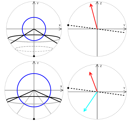
Figure 21: Unit sphere (outline dotted), centred on the galaxy centre, with the X and Y axes on the galactic plane, and the Z-axis along the symmetry axis of the disc. The direction to the observer is marked by the small black filled circle in the semi-plane Y$<$0, Z$>$0, and is inclined by i=82^∘ with respect to the Z-axis. In this way, the X-axis corresponds to the apparent major axis of the galaxy. The upper panels represent the case $\beta$=25^∘ and V_wind=2400 km s^-1, while the lower panels represent the case $\beta$=45^∘ with the same V_wind. This wind speed corresponds to $\phi$=69.64^∘. The left panels offer a view of the unit sphere from the Z-axis. The blue circles are the intersection with the sphere of the cones $\beta$=const. The black and gray ellipses are the intersection with the unit sphere of the semi-cone $\phi$=const. directed towards the observer. The gray section is the half of the ellipse laying at Z$<$0, i.e. at the opposite side of the galaxy disc in this view. The right panels show the same configurations projected on the YZ plane. The dashed line is the line of sight. The dot-dashed ellipse in the upper-left panel is the intersection of the unit sphere with the cone corresponding to V_wind=1100 km s^-1, an example of a forbidden configuration. The arrows represent projections of the ICM wind (see text).

In the bottom panels of the same figure (corresponding to the case $\beta=$45^∘ and $\phi\sim$70^∘) the wind cone intersects the $\phi$-cone in both hemispheres. There are intersections in the Z$>$0 hemisphere at $\theta_{1}$,$\theta_{2}$ (=-24.3^∘, 204.3^∘; black lines), and for Z$<$0 the intersections take place at $\theta_{3}$,$\theta_{4}$ (=-54.4^∘, 234.4^∘ gray lines). Rotating the model by $\theta_{1}$ or $\theta_{2}$, allows us, as before, to see the model from the correct point of view. But in this case the model can also be rotated around the Z-axis by $\theta_{3}$ or $\theta_{4}$.

The second case corresponds to the cyan wind vector in the bottom-right panel and represents an example of case B. To reach this configuration, the model should be first rotated by 180^∘ around the X-axis.

The coordinate transformations needed in the above process are the following. Let $\beta$ be the angle of the wind with respect to the symmetry axis of the galaxy and $i$ the inclination angle of the galaxy (plane of the sky to galaxy disc). First we move the symmetry axis of the galaxy into the Z-axis with a clock-wise rotation of $\beta$ around the Y-axis. In this way, the wind lies on the (X,Z) plane. The second step is to move the wind vector in a direction in which the wind speed projects into $\overrightarrow{V}_{gal}$. It can be shown that his is achieved by a rotation around the Z-axis by an angle $\theta$ given by

$$cos\ \theta=-\frac{cos\ \phi+k\ cos\ \beta\ cos\ i}{sin\ \beta\ sin\ i}\ \ \ ,$$

where $k=-1$ for case A and $k=1$ for case B. For each $k$ this equation has two solutions: $\theta_{1}=arcos(cos\ \theta)$ and $\theta_{2}=\pi-\theta_{1}$. As a result, when only case A is allowed, there are two possible viewing angles (or ‘projections’), while when both cases A and B are allowed, the possible projections are four.

Other transformations are possible that do not change the physics of the models, but given that we fixed the position of the line of sight in the YZ plane, the only remaining meaningful transformation is a reflection with respect to that plane. This corresponds to an inversion of the X-axis and to the change of sign of the corresponding velocity component of the model particles. This transformation makes the projection of the models on the sky to reflect with respect to the apparent major axis, and may become useful to match the models to the observed orientation of the galaxy, when this is not achievable with a simple rotation. In the present case this transformation was not needed.

Cases A and B represent two quite different observing conditions. In case A, the wind acts on the disc side opposite to the observer, in such a way that the outflowing gas overlays the disc. In case B the opposite is true, and part of the outflowing gas is hidden by the disc.

Finally, we notice that not all combinations of parameters lead to an observable configuration. An example is illustrated by the dot-dashed ellipse in the top-left panel of Fig. 21, which is the intersection with the unit sphere of a $\phi$-cone corresponding to V_wind=1100 km s^-1. This cone has no intersection with the $\beta$-cone corresponding to $\beta$=25^∘. This means that there is no possible orientation such that this configuration would lead to the observed line-of-sight velocity of our galaxy.

A.2 Simulating the observations

The end product of the previous process is a matrix (x_i,y_i,V_i; i=1,…,N_particles), where (x,y) are coordinates in the plane of the sky (x is along the apparent major axis), y is normal to x, V is the radial velocity and N_particles is the number of particles in the simulation.

To reproduce the effect of the seeing we substituted each particle by a Gaussian distribution with the FWHM equal to the seeing. In each surface element of the plane of the sky (see below), we computed the surface density of particles $\Sigma$ as the sum of the contributions from the Gaussians and the radial velocity as the weighted average of the individual velocities.

To speed-up the computation, we truncated the contribution of each particle at 10$\times\sigma_{Gauss}$. This computation was performed on a grid of points spaced by 0.1${\prime\prime}$ on the sky, which we verified to offer a reasonable compromise between accuracy and computation speed. The points in the plane of the sky were eventually sampled in $1{\prime\prime}\times 1{\prime\prime}$ bins, matching the spatial binning of the data, and rotated to the position angle of the major axis of our galaxy.

References

- Abadi et al. (1999) Abadi M. G., Moore B., & Bower R. G., 1999, MNRAS, 308, 947
- Abramson et al. (2011) Abramson A., Kenney J. D. P., Crowl H. H. et al., 2011, AJ, 141, 164
- Akimoto et al. (2003) Akimoto F., Kondou K., Furuzawa A., Tawara Y., Yamashita K., 2003, ApJ, 596, 170
- Allen et al. (1991) Allen D. P., Norris R. P., Meadows V. S., Roche P. F., 1991, MNRAS, 248, 528
- Ascasibar & Diego (2008) Ascasibar Y. & Diego J. M., 2008, MNRAS, 383, 369
- Athanassoula & Misiriotis (2002) Athanassoula E. & Misiriotis A., 2002, MNRAS, 330, 35
- Baes et al. (2003) Baes M., Davies J. I., Dejonghe H., et al., 2003, MNRAS, 343, 1081
- Baldry et al. (2006) Baldry I. K., Balogh M. L., Bower R. G., et al., 2006, MNRAS, 373, 469
- Balogh et al. (2000) Balogh M. L., Navarro J. F., & Morris S. L., 2000, ApJ, 540, 113
- Bamford et al. (2009) Bamford S. P., Nichol R. C., & Baldry I. K., 2009, MNRAS, 393, 1324
- Bardelli at al. (1996) Bardelli S., Zucca E., Malizia A., et al., 1996, A&A, 305, 435
- Bardelli at al. (1998) Bardelli S., Pisani A, Ramella M., Zucca E., Zamorani G., 1998, MNRAS, 300, 589
- Barnes & Hut (1986) Barnes J. & Hut P., 1986, Nature, 324, 446
- Barnes & Hernquist (1991) Barnes J. E. & Hernquist L. E., 1991, ApJ, 370, 65L
- Bekki (2001) Bekki K., 2001, ApJ, 546, 189
- Bekki et al. (2002) Bekki K., Couch W. J., & Shioya Y., 2002, ApJ, 577, 651
- Bekki (2009) Bekki K., 2009, MNRAS, 399, 2221
- Boselli & Gavazzi (2006) Boselli A. & Gavazzi G., 2006, PASP, 118, 517
- Bosma (1981) Bosma A., 1981, AJ, 86, 12
- Blanton et al. (2005) Blanton M. R., Eisenstein D., Hogg D. W., et al., 2005, ApJ, 629, 143
- Bureau & Athanassoula (2005) Bureau M. & Athanassoula L., 2005, ApJ, 626, 159.
- Butcher & Oemler (1984) Butcher H. & Oemler Jr. A., 1984, ApJ, 284, 426
- Byrd & Valtonen (1990) Byrd G. & Valtonen M., 1990, ApJ, 350, 89
- Cardelli et al. (1989) Cardelli J. A., Clayton G. C., & Mathis J. S., 1989, ApJ, 345, 245
- Cappellari & Copin (2003) Cappellari M. & Copin Y., 2003, MNRAS, 342, 345
- Chemin et al. (2005) Chemin L., Cayatte V., Balkowski C., et el., 2005, A&A, 436, 469
- Chung & Bureau (2004) Chung A. & Bureau M., 2004, AJ, 127,3192
- Chung et al. (2007) Chung A., van Gorkom J. H., Kenney J. D. P., Vollmer B., 2007, ApJ, 659L, 115
- Chung et al. (2009) Chung A., van Gorkom J. H., Kenney J. D. P., Crowl H., Vollmer B., 2009, AJ, 138, 1741
- Cid Fernandes et al. (2005) Cid Fernandes R., Mateus A., Sodré, Stasińska G., Gomes J. M., 2005, MNRAS, 358 363
- Conselice et al. (2005) Conselice C. J., Bundy K., Ellis R. S, Brichmann J., 2005, AJ, 628, 160
- Cortés et al. (2006) Cortés J. R., Kenney J. D. P., & Hardy E., 2006, AJ, 131, 747
- Cortese et al. (2007) Cortese L., Marcillac D., Richard J., et al., 2007, MNRAS, 376, 157
- Cortese et al. (2010) Cortese L., Davies J. I. Pohlen M., Baes M., et al., 2010, A&A, 518, 49
- Courteau et al. (2003) Courteau S., Andersen D.R., Bershady M.A., MacArthur L.A., Rx H.-W., 2003, ApJ, 594, 208
- Clarke et al. (1998) Clarke C. J., Kinney A. L., & Pringle J. E., 1998, ApJ, 495, 189
- Cowie & Songalia (1977) Cowie L. L. & Songalia A., 1977, Nature, 266, 501
- Crowl et al. (2005) Crowl H. H., Kenney J. D. P., van Gorkom J. H., Vollmer, B., 2005, AJ, 130, 65
- Crowl & Kenney (2006) Crowl H. H. & Kenney J. D. P. 2006, ApJ, 649L 75
- Crowl & Kenney (2008) Crowl H. H. & Kenney J. D. P. 2008, AJ, 136, 1623
- Dale et al. (1999) Dale D. A., Giovaneli R., Haynes M. P., Hardy E., Campusano J. E., 1999, ApJ, 118, 1468
- Dale et al. (2001) Dale D. A., Giovaneli R., Haynes M. P., Hardy E., Campusano J. E., 2001, AJ, 121, 1886
- de Naray et al. (2009) de Naray R. K., Zagursky M. J., McGaugh S. S., 2009, AJ, 138, 1082
- Diehl & Statler (2006) Diehl S. & Statler T. S., 2006, MNRAS, 368, 497
- Dopita & Sutherland (2003) Dopita M. A. & Sutherland R. S., 2003, Astrophysics of the Diffuse Medium, Springer-Verlag Berlin Heidelberg 2003
- Dopita et al. (2007) Dopita M. A., Hart J., McGregor P., Oates P., Bloxham, G., Jones D., 2007, Ap&SS, 310, 255
- Dopita et al. (2010) Dopita M. A., Rhee J., Farage C. et al., 2010, Ap&SS, 327, 245
- Dressler (1980) Dressler A., 1980, ApJ, 236, 351
- Dressler et al. (1997) Dressler A., Oemler A. Jr., Couch W. J., et al. 1997, ApJ, 490, 577
- Dressler et al. (1999) Dressler A., Smail I., Poggianti B. M., et al. 1999, ApJS, 122, 51
- Dressler et al. (2004) Dressler A., Oemler A. Jr., Poggianti B. M., et al. 2004, ApJ, 617, 867
- Driver et al. (2008) Driver S.P., Popescu C.C., Tuffs R.J., et al., 2008, ApJ, 678, L101
- Ellison et al. (2011) Ellison S.L., Preethi N., Patton D.R., et al., 2011, MNRAS, 416, 2182
- Emsellem et al. (2007) Emsellem E., Cappellari M., Krajnović D., et al., 2007, MNRAS, 379, 401
- Farage et al. (2010) Farage C. L., McGregor P. J., Dopita M. A., Bicknell G. V., 2010, ApJ 724, 267
- Fathi et al. (2005) Fathi K., van de Ven G., Peletier R.F., et al., 2005, MNRAS, 364, 773
- Fischera & Dopita (2005) Fischera J. & Dopita M. A., 2005, ApJ, 619, 340
- Fossati et al. (2012) Fossati M., Gavazzi G., Boselli, Fumagalli M., 2012, A$A, 544, 128
- Fujita & Nagashina (1999) Fujita Y. & Nagashina M., 1999, ApJ, 516, 619
- Gavazzi et al. (2001) Gavazzi G., Boselli A., Mayer L., et al., 2001, 563L, 23
- Gingold & Monaghan (1977) Gingold R. A. & Monaghan J. J., 1977, MNRAS, 181, 375
- Giovanelli & Haynes (2002) Giovanelli R. & Haynes M. P., 2002, ApJL, 571, 107
- Graham & Worley (2008) Graham A. W. & Worley C. C., 2008, MNRAS, 388, 1708
- Grevesse et al. (2010) Grevesse N., Asplund M., Sauval A. J., Scott P., 2010, Ap&SS, 328, 179
- Gunn & Gott (1972) Gunn J. E. & Gott J. R. III, 1972, ApJ, 176, 1
- Haines et al. (2006) Haines C. P., Merluzzi P., Mercurio A., et al. 2006, MNRAS, 371, 55
- Haines et al. (2007) Haines C. P., Gargiulo A., La Barbera F., Mercurio A., Merluzzi P., Busarello G., 2007, MNRAS, 381, 7
- Haines et al. (2009) Haines C. P., Smith G. P., Egami E., et al., 2009, ApJ, 704, 126
- Haines et al. (2011a) Haines C. P., Busarello G., Merluzzi P., et al., 2011a, MNRAS, 412, 127, Paper II
- Haines et al. (2011b) Haines C. P., Busarello G., Merluzzi P., et al., 2011b, MNRAS, 412, 145, Paper III
- Haines et al. (2011c) Haines C. P., Merluzzi P., Busarello G., et al., 2011c, MNRAS, 417, 2831
- Haynes et al. (2007) Haynes M. P., Giovanelli R., & Kent B. R., 2007, ApJ, 665L, 19
- Hernquist (1990) Hernquist L., 1990, ApJ, 356, 359
- Hoopes et al. (2005) Hoopes C.G., Heckman T.M., Strickland D.K., et al., 2005, Apj, 619, L99
- Hundaverdi et al. (2010) Hundaverdi M., Bozkurt M., & Ercan N., 2010, ASP Conference Series, Vol. 424, 330
- Irwin & Sarazin (1996) Irwin J. A. & Sarazin C. L., 1996, ApJ, 471, 683
- Jáchym et al. (2009) Jáchym P., Köppen J., Palous J., Combes F., 2009, A&A, 500, 693
- James et al. (2008) James P. A., Prescott M., & Baldry I. K., 2008, A&A, 484, 703
- Jiménez-Vicente et al. (2010) Jiménez-Vicente J., Mediavilla E., Castillo-Morales A., Battener E., 2010, MNRAS, 406, 181
- Kapferer et al. (2009a) Kapferer W., Kronberger T., Ferrari C., Riser T., Schindler S., 2009a, MNRAS, 389, 1405
- Kapferer et al. (2009b) Kapferer W., Sluka C., Schindler S., Ferrari C., Ziegler B., 2009b, A&A, 499, 87
- Katz et al. (1996) Katz N., Weinberg D. H, Hernquist L., 1996, ApJS, 105, 19
- Kauffmann et al. (2003) Kauffmann G., Heckman T. M., Tremonti C., et al. 2003, MNRAS, 346, 1055
- Kauffmann et al. (2004) Kauffmann G., White S. D. M., Heckman T. M., et al., 2004, MNRAS, 353, 713
- Kenney & Koopmann (1999) Kenney J. D. & Koopmann R., 1999, AJ, 117, 181
- Kenney et al. (2004) Kenney J. D. P., van Gorkom J. H., & Vollmer B., 2004, AJ, 127, 3361
- Kenney et al. (2008) Kenney J. D. P., Tal T., Crowl H. H., Feldmeier J., Jacoby G. H., 2008, ApJ, 687L, 69
- Kennicutt (1983) Kennicutt R. C. Jr., 1983, ApJ, 272, 54
- Kennicutt et al. (1994) Kennicutt R. C. Jr., Tamblyn P., Congdon C. E., 1994, ApJ, 435, 22
- Kennicutt (1998) Kennicutt R. C. Jr., 1998, ApJ, 498, 541
- Kewley et al. (2001) Kewley, L. J., Heisler, C. A., Dopita, M. A., Lumsden, S. 2001, ApS, 132, 37
- Kewley et al. (2006) Kewley, L. J., Groves, B., Kauffmann G., Heckman T., 2006, MNRAS, 372, 961
- Kim et al. (2008) Kim D.-W., Kim E., Fabbiano G., Trinchieri G., 2008, ApJ, 688, 931
- Kimura et al. (2003) Kimura H., Mann I., & Jessberger E. K., 2003, ApJ, 582, 846
- Koleva et al. (2008) Koleva M., Prugniel Ph., Ocvirk P., Le Borgne D., Soubrian C., 2008, MNRAS, 385, 1998
- Koleva et al. (2009) Koleva M., Prugniel Ph., Bouchard A., Wu Y., 2009, A&A, 501, 1269
- Koopmann et al. (2008) Koopmann R. A., Giovanelli R., Haynes M. P., et al., 2008, ApJ 682L, 85
- Kormendy & Bender (2012) Kormendy J. & Bender R., 2012, ApJSS, 198, 2
- Kregel et al. (2004) Kregel M., van der Kruit P. C., & Freeman K. C., 2004, MNRAS, 351, 1247
- Kronberger et al. (2006) Kronberger T., Kapferer W., Schindler S., et al., 2006, A&A, 458, 69
- Kronberger et al. (2007) Kronberger T., Kapferer W., Schindler S., Ziegler B. L., 2007, A&A, 473, 761
- Kronberger et al. (2008a) Kronberger T., Kapferer W., Ferrari C., Unterguggenberger S., Schindler S., 2008a, A&A, 481, 337
- Kronberger et al. (2008b) Kronberger T., Kapferer W., Unterguggenberger S., Schindler S., Ziegler B. L., 2008b, A&A, 483, 783
- Kroupa (2001) Kroupa P., 2001, MNRAS, 322, 231
- Larson et al. (1980) Larson R. B., Tinsley B. M., & Caldwell C. M., 1980, ApJ, 237, 692
- Leitherer et al. (1999) Leitherer C., Schaerer D., Goldader J. D., et al., 1999, ApJS, 123, 3
- Leonardi & Rose (1996) Leonardi A. J. & Rose J. A., 1996, AJ, 111, 182
- Leroy et al. (2008) Leroy A. K., Walter F., Brinks E., et al., 2008, AJ, 136, 2782
- Lewis et al. (2002) Lewis I., Balogh M., De Propris R., et al. 2002, MNRAS, 334, 673
- Lucy (1977) Lucy L. B., 1977, AJ, 82, 1013
- MacArthur et al. (2009) MacArthur L. A., González J. J., & Courteau S., 2009, MNRAS, 395, 28
- Machacek et al. (2006) Machacek M., Jones C., Forman W. R., Nulsen P., 2006, ApJ, 644, 155
- Marcolini et al. (2003) Marcolini A., Brighenti F., & D’Ercole A., 2003, MNRAS, 345, 1329
- McCarthy et al. (2008) McCarthy I. G., Frenk C. S., Font A. S., et al., 2008, MNRAS, 383, 593
- Mercurio et al. (2006) Mercurio A., Merluzzi P., Haines C. P., et al. 2006, MNRAS, 368, 109
- Merluzzi et al. (2010) Merluzzi P., Mercurio A., Haines C. P., Smith R. J., Busarello G., Lucey J. R., 2010, MNRAS, 402, 753, Paper I
- Miller (2005) Miller N. A., 2005, AJ, 130, 2541
- Mo et al. (1998) Mo H. J., Mao S., & White S. D. M., 1998, MNRAS, 295, 319
- Monreal-Ibero et al. (2010) Monreal-Ibero A., Arribe S., Colina L., et al., 2010, A&A, 517, 28
- Moore et al. (1996) Moore B., Katz N., Lake G., Dressler A., Oemler A., 1996, Nature, 379, 613
- Moster et al. (2011) Moster B. P., Macciò A. V., Somerville R. S. Naab T., Cox T. J., 2011, MNRAS, 415, 3750
- Moustakas et al. (2010) Moustakas J., Kennicutt R. C. Jr., & Tremonti C. A., 2010, ApJS, 190, 233
- Murakami et al. (2007) Murakami H., Baba H., Barthel P., et al., 2007, PASJ, 59, S369
- Nulsen (1982) Nulsen P. E. J., 1982, MNRAS, 198, 1007
- Oh et al. (2012) Oh S., Oh K., & Yi S.K., 2012, ApJS, 198, 4
- Oosterloo & van Gorkum (2005) Oosterloo T. & van Gorkom J., 2005, A&A, 437L, 190
- Ocvirk et al. (2006) Ocvirk P., Pichon C., Lancon A., Thiébaut E., 2006, MNRAS, 365, 46
- Peng et al. (2010) Peng C. Y., Ho L. C., Impey C. D., Rix H-W., 2010, ApJ, 139, 2097
- Pracy et al. (2009) Pracy M. B., Kanschner H., Couch W. J., et al. 2009, MNRAS, 396, 1349
- Pracy et al. (2012) Pracy M. B., Owers M. S., Couch W. J., et al., 2012, MNRAS, 420, 2232
- Proust et al. (2006) Proust D., Quintana H., Carrasco E. R., et al., 2006, A&A 133, 447
- Rich et al. (2010) Rich J. A., Dopita M. A., Kewley L. J., Rupke D. S. N., 2010, ApJ, 721, 517
- Rich et al. (2011) Rich J. A., Kewley L. J., & Dopita M. A., 2011, Apj, in press.
- Rieke et al. (2009) Rieke G. H., Alonso-Herrero A., Weiner B. J., et al., 2009, ApJ, 692, 556
- Roediger & Hensler (2005) Roediger E. & Hensler G., 2005, A&A, 433, 875
- Roediger & Brüggen (2006) Roediger E. & Brüggen M., 2006, MNRAS, 369, 567
- Roediger & Brüggen (2008) Roediger E. & Brüggen M., 2008, MNRAS, 388, 465
- Rose (1985) Rose J. A., 1985, AJ, 90, 1927
- Rossetti et al. (2007) Rossetti M., Ghizzardi S., Molendi S., Finoguenov A., 2007, A&A, 463, 839
- Sánchez et al. (2011) Sánchez S. F., Rosales-Ortega F. F., Kennicutt R. C., et al., 2011, MNRAS, 410, 313
- Sánchez-Blázquez et al. (2006) Sánchez-Blázquez P., Peletier R. F., Jiménez-Vicente J., et al., 2006, MNRAS, 371, 703
- Sanderson & Ponman (2010) Sanderson A. J. R. & Ponman T. J., 2010, MNRAS, 402, 65
- Schlegel et al. (1998) Schlegel D. J., Finkbeiner D. P., & Davis M., 1998, ApJ, 500, 525
- Smith et al. (2004) Smith R. J., Hudson M. J., Nelan J. E., 2004, AJ. 128, 1558
- Smith et al. (2007) Smith R. J., Lucey J. R., & Hudson M. J., 2007, MNRAS, 381, 1035
- Smith et al. (2010) Smith R. J., Lucey J. R., Hammer D., 2010, MNRAS, 408, 1417
- Springel & Hernquist (2003) Springel V. & Hernquist L., 2003, MNRAS, 339, 289
- Springel et al. (2005) Springel V., Di Matteo T., & Hernquist L., 2005, MNRAS, 361, 776
- Springel (2005) Springel V., 2005, MNRAS, 364, 1105
- Steinhauser et al. (2012) Steinhauser D., Haider D., Kapferer W., Schindler S., 2012, A&A, 544, A54
- Storey & Zeippen (2000) Storey P. J. & Zeippen C. J., 2000, MNRAS, 312, 813
- Sun & Vikhlinin (2005) Sun M. & Vikhlinin A., 2005, ApJ, 621, 718
- Sun et al. (2006) Sun M., Jones C., Forman W., et al., 2006, ApJ, 637L, 915
- Sun et al. (2010) Sun M., Donahue M., Roediger E., et al., 2010, ApJ, 78, 946
- Sutherland & Dopita (1993) Sutherland R. S. & Dopita M. A., 1993, ApJS, 88, 253
- Toomre & Toomre (1972) Toomre A. & Toomre J., 1972, ApJ, 178, 623
- Tonnesen & Bryan (2009) Tonnesen S. & Bryan G. L., 2009, ApJ, 694, 789
- Tonnesen & Bryan (2010) Tonnesen S. & Bryan G. L., 2010, ApJ, 709, 1218
- Tonnesen & Bryan (2012) Tonnesen S. & Bryan G. L., 2012, MNRAS, 422, 1609
- Urban e al. (2011) Urban O., Werner N., Simionescu A., Allen S. W.,Böhringer H., 2011, MNRAS, 414, 2101
- Valotto & Giovanelli (2004) Valotto C. & Giovanelli R., 2004, AJ, 128, 115
- van Dokkum (2001) van Dokkum P. G., 2001, PASP, 113, 1420
- Vazdekis et al. (2010) Vazdekis A., Sánchez-Blázquez P., Falcón-Barroso J., et al., 2010, MNRAS, 404, 1639
- Veilleux & Osterbrock (1987) Veilleux S. & Osterbrock D. E. 1987, ApJs, 63, 295
- Veilleux et al. (2005) Veilleux S., Cecil G., & Bland-Hawthorn J., 2005, ARA&A, 43, 769
- Veilleux et al. (2010) Veilleux S., Weiner B.J., Rupke D.S.N., et al., 2010, AJ, 139, 145
- Vogt et al. (2004) Vogt N. P., Haynes M. P., Giovanelli R., Herter T., 2004, AJ, 127, 3300
- Vollmer et al. (2000) Vollmer B., Marcellin M., Amram P., et al., 2000, A&A, 364, 532
- Vollmer et al. (2005) Vollmer B., Braine J., Combes F., Sofue Y., 2005, A&A, 441, 473
- Vollmer et al. (2008) Vollmer B., Soida M., Chung A., et al., 2008, A&A, 483, 89
- Vollmer et al. (2009) Vollmer B., Soida M., Chung A., et al., 2009, A&A, 496, 669
- Vollmer et al. (2010) Vollmer B., Soida M., Chung A., et al., 2010, A&A, 512, 36
- Wang et al. (2004) Wang Q. D., Owen F., & Ledlow, 2004, ApJ, 611, 821
- Williams et al. (2011) Williams B. F., Dalcanton J. J.; Johnson L. C., et al., 2011, ApJ, 734, L22
- Yagi et al. (2007) Yagi M., Komiyama Y., Yoshida M. et al., 2007, ApJ, 660, 1209
- Yagi et al. (2010) Yagi M., Yoshida M., Komiyama Y., et al., 2010, AJ, 140, 1814
- Yoshida et al. (2002) Yoshida M., Yagi M., Okamura S., et al. 2002, ApJ, 567, 118