Percolation thresholds on 3-dimensional lattices with 3 nearest neighbors

Abstract

We present a study of site and bond percolation on periodic lattices with 3 nearest neighbors per site. We have considered 3 lattices, with different symmetries, different underlying Bravais lattices, and different degrees of longer-range connections. As expected, we find that the site and bond percolation thresholds in all of the 3-connected lattices studied here are significantly higher than in diamond. Interestingly, thresholds for different lattices are similar to within a few percent, despite the differences between the lattices at scales beyond nearest and next-nearest neighbors.

I Introduction

Percolation is one of the simplest phase transitions known: sites on a lattice are occupied at random until there is a path that can be traversed from one end of the lattice to the other, traveling only neighbor-to-neighbor on occupied sitesStauffer and Aharony (1994). The set of sites along this path or connected to this path (via neighbor-to-neighbor steps along occupied sites) is called the spanning cluster. In the limit of a large system size (linear dimension $L\gg 1$), the probability of forming a spanning cluster via random occupation of sites goes to zero below a critical occupation probability per site $p_{c}$ and unity above $p_{c}$. Percolation models have been used to study a great many phenomena, from transport in porous media to biological systems to gelationSahimi (1994).

A well-known trend in percolation on periodic 3D lattices is that $p_{c}$ increases as the coordination number $z$ (number of nearest neighbors per site) decreasesGalam and Mauger (1996). (See Table 1 near the end for examples and more references.) This trend arises from the fact that, when there are fewer neighbors per site, there are fewer ways to navigate around an obstacle. Consequently, more sites have to be occupied to ensure a path spanning from one end of the system to the other. To our knowledge, the lowest coordination number studied for percolation on simple 3D lattices is $z=4$, the most prominent example being the diamond lattice with $p_{c}\approx 0.43$ for site percolationSilverman and Adler (1990) and $\approx 0.388$ for bond percolationVyssotsky et al. (1961).

However, $z=4$ is not the lowest possible coordination number. The lowest possible non-trivial coordination number is $z=3$, and this coordination number has been realized in interesting families of 3D lattices, namely the $(n,3)$ families of lattices studied by A. F. WellsWells (1977). The $3$ refers to the number of nearest neighbors (bonds) per site, and $n$ is the smallest number of steps that one would have to take along the lattice sites to return to the same point. In lattice families with multiple members, $(n,3)$ is followed by a letter, e.g. $(10,3)$-a, $(10,3)$-b, etc. A total of 30 lattices have been identified in these families, with $n$ values of 7, 8, 9, 10, and 12. The $(n,3)$ lattices offer a chance to study the interplay between nearest neighbors, higher-level connectivity (via $n$), and other aspects of lattice geometry (e.g.  the differences between, say, $(10,3)$-a and $(10,3)$-b) for the lowest non-trivial $z$ value. We are only aware of one study of percolation on lattices in this family, namely the $(10,3)$-a latticePaterson et al. (2002), and that study focused on invasion percolation and trapping, rather than the standard site and bond percolation problems.

Recently, the $(10,3)$-a lattice has attracted additional attention because of its unusually high symmetry, possessing a property known as “strong isotropy.”Sunada (2008) Only one other 3D lattice (diamond), shares this property with $(10,3)$-a. The $(10,3)$-a structure is observed in a number of interesting systems, e.g.  block copolymersBates (2005), and it has been proposed as a possible structure for a metastable phase of carbonItoh et al. (2009). Motivated by this recent attention to $(10,3)$-a and related lattices, as well as the general question of how high the percolation threshold can be for a 3D lattice with $z=3$, we have studied 3 lattices in this family: $(10,3)$-a, its close relative $(10,3)$-b, and $(8,3)$-a. These particular lattices span multiple $n$ values, and are especially easy to study because they can be realized with bonds of uniform length and $120^{\circ}$ bond angles, making them easy to construct with ball and stick models.

In what follows, we first discuss the geometries of our three representative lattices in their simplest forms: equal bond lengths and $120^{\circ}$ bond angles. We illustrate deformations of the lattices that preserve the topology (connections between nearest neighbors) but enable a mapping onto a cubic lattice, for convenience in enumerating sites in a calculation. We then summarize key features of the Newman-Ziff algorithmNewman and Ziff (2001) used to determine the site and bond percolation thresholds of the lattices, and present the computed percolation thresholds. Finally, we compare our results with other lattices.

II The lattices under study

II.1 The (10, 3)-a lattice

The (10, 3)-a lattice (shown in Fig. 1(a)) can be thought of as a body-centered cubic (bcc) lattice with a 4-atom basis. If we work in a coordinate system where the sites of the bcc lattice are at the corners of a cube, one site is at the origin $(0,0,0)$, and the edges are of unit length and parallel to the standard $x$, $y$, and $z$ axes, then the 3 other atoms in the basis are at $\left(0,-\frac{1}{4},\frac{1}{4}\right)$, $\left(-\frac{1}{4},\frac{1}{4},0\right)$, and $\left(\frac{1}{4},0,-\frac{1}{4}\right)$. The atoms correspond to sites 0 through 3 in the figure (i.e.  the atoms at the origin and its 3 nearest neighbors), they sit in the (111) plane, and the bonds to them are separated by $120^{\circ}$ angles.

In percolation theory, the geometry of the bonds is less important than the presence of the bonds. A deformation of the lattice and bonds that preserves the connections between sites will not change the percolation threshold of the lattice. In the Newman-Ziff algorithm that we used, all of the relevant information on the lattice is stored in the "nn" array, which contains the labels of the nearest neighbors bonded to each site in the lattice. For convenience in enumerating sites, we have deformed the lattice to fit onto a simple cubic grid, while preserving the bonding structure of the lattice. Our numbering system for sites, and the deformations used to fit them onto a cubic grid, are shown in Fig. 1(b) and Fig. 1(c).

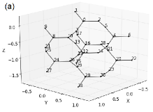
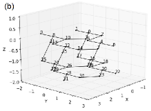
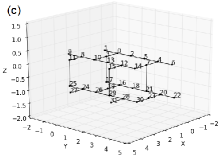
Figure 1: (a) The (10,3)-a lattice, with sites numbered. (b) and (c) The deformations used to map the lattice onto a cubic grid for computational convenience.

II.2 The (10,3)-b lattice

The (10,3)-b lattice is unusual, because even if we specify unit bond lengths and 120 degree bond angles we still have an unconstrained structural degree of freedom: Suppose that we define the positions of all of the lattice sites and also the basis. We can then deform the lattice in a manner that uniformly changes the spacing between lattice planes, while also displacing the atoms in the lattice planes, without changing any bond lengths or bond angles. We have chosen to describe this lattice in a form that maximizes the symmetry, as this form lends itself to easier visualization with ball-and-stick models. In this form, the lattice is body-centered tetragonal, with lattice vectors $(\sqrt{3},0,0)$, $(0,\sqrt{3},0)$, and $\left(\frac{\sqrt{3}}{2},\frac{\sqrt{3}}{2},3\right)$.

The 4-atom basis is more complicated. Instead of a central atom with 3 neighbors, the basis is a chain of 4 atoms, located at $(0,0,0)$, $\left(0,\frac{\sqrt{3}}{2},\frac{1}{2}\right)$, $\left(0,\frac{\sqrt{3}}{2},\frac{3}{2}\right)$, and $\left(-\frac{\sqrt{3}}{2},\frac{\sqrt{3}}{2},2\right)$. These correspond to sites 0 through 3 in the figure. As before, we also deform this lattice to represent it on a simple cubic grid. The numbering system and deformation steps are illustrated in Fig. 2(b) and (c).

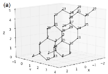
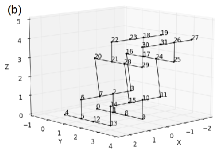
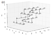
Figure 2: (a) The (10,3)-b lattice, with sites numbered. (b) and (c) The deformations used to map the lattice onto a cubic grid for computational convenience

II.3 The (8,3)-a lattice

We realized the (8,3)-a lattice, shown in Fig. 3(a), in a structure that has hexagonal symmetry, with lattice vectors $(-5/2,\sqrt{3}/6,2\sqrt{2/3})$, $(5/2,\sqrt{3}/6,2\sqrt{2/3})$, and $(0,4\sqrt{3}/3,\sqrt{2/3})$. The $x$ axis is the axis of hexagonal symmetry.

The (8, 3)-a lattice has a six-atom basis, with unit bond lengths and atoms located at $(0,0,0)$, $(0,-\sqrt{3}/3,-\sqrt{2/3})$, $(1/2,-5\sqrt{3}/6,-\sqrt{2/3})$, $(3/2,-5\sqrt{3}/6,-\sqrt{2/3})$, $(2,-\sqrt{3}/3,-\sqrt{2/3})$, and $(2,0,0)$. These correspond to sites 0 through 5 in the figure. The steps used to deform the (8,3)-a lattice so that it fits onto a cubic grid are illustrated in Fig. 3(b) and (c).

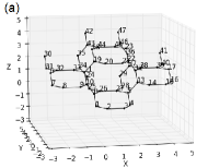
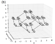
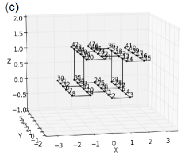
Figure 3: (a) The (8,3)-a lattice, with sites numbered. (b) and (c) The deformations used to map the lattice onto a cubic grid for computational convenience

III Simulations

III.1 Description of the algorithm

We used the Newman-Ziff algorithm for identifying the percolation threshold of finite-sized clustersNewman and Ziff (2001). In brief, the algorithm works by occupying sites (or bonds) on a lattice of $N$ one-at-a-time in a random order. Relationships between sites are defined in the array nn, which indicates the site numbers for the nearest neighbors of each site. At each step, after a site is occupied we check whether the occupation of the $n$th site produces a cluster that wraps around the entire system. Each cluster is assigned a “pointer” to a root (or parent) site, corresponding to the first site in the cluster, and also a vector that points in the direction of the parent site. As clusters grow and merge, pointers and vectors are updated to the root of the largest cluster involved in the merger. Wrapping is detected when a newly-occupied site (1) joins two portions of the same cluster and (2) the vectors going from the joined portions of the cluster to the root differ by something other than the displacement vector between the sites. We consider wrapping between parallel faces of the computational volume (i.e.  along the $x$, $y$, and $z$ directions) as well as diagonal wrapping. (See the paper by Newman and ZiffNewman and Ziff (2001) for more details.) The iteration ends when wrapping is detected. Another lattice is then generated, and the process is repeated, until $N_{L}$ lattices (typically $10^{3}$ in our work) have been generated. Bond percolation is handled in a completely analogous manner, substituting bonds for sites. Two bonds are considered neighbors if they touch the same site.

This process generates a plot of wrapping probability $R_{L}$ vs. occupation fraction $\phi=n/N$, where $L$ refers to the linear dimension of the lattice. In order to determine $R_{L}$ as a function of occupation probability (the usual quantity of interest in percolation theory), it is necessary to convolve $R_{L}$ with a binomial distribution:

$$R_{L}(p)=\sum_{n=0}^{N}\left(\begin{array}[]{c}N\\ n\end{array}\right)p^{n}(1-p)^{N-n}R_{L}(n)$$ (3)

Eq. (3) amounts to a weighted sum over all possible realizations of an $N$-site lattice with site occupation probability $p$. The number of realizations that wrap with $n$ occupied sites enters the sum via $R_{L}(n)$. Different occupation numbers $n$ will have different likelihoods of being realized at the same occupation probability $p$, i.e.  different degeneracies, and this enters the sum via the binomial distributions. Occupation numbers that are not close to $N\cdot p$ are unlikely, and hence get low weight from the binomial distribution.

To implement the algorithm we closely followed the code example given in the paper by Newman and Ziff, implementing it in Python 2.7 on a quad-core Intel processor in Linux (Ubuntu 12.04). We checked our code by determining the site and bond percolation thresholds of the 2D square, 2D honeycomb, and 3D simple cubic lattices. Adapting the code to the lattices under study only required modification to the function that identifies the nearest neighbors of each site, as well as the vectors from each site to its neighbors. To validate the output for the lattices under study, we generated lattices with small numbers of sites ($\approx 30$) and had the code output the list of occupied sites when wrapping occurred. We verified by hand that (1) there was a cluster that wrapped the lattice, and (2) the removal of the most recently occupied site would cause the cluster to not wrap.

Given a plot of the wrapping probability $R_{L}(p)$ for different lattice sizes $L$, it is possible to obtain an estimate of the percolation threshold $p_{c}$ by looking for the point where the plot crosses over from low wrapping probability to high (e.g.  the steepest point on the plot). An example for the (10,3)-a lattice is shown in Fig. 4. For sufficiently large system sizes, this estimate of $p_{c}$ can be quite accurate. More efficient approaches can obtain high precision and accuracy by comparing $R_{L}(p)$ plots for several different system sizes $L$. One common way of comparing plots at different sizes is to use the scaling relation $|p_{c}(L)-p_{c}|\propto L^{-\omega-\nu}$, where $p_{c}(L)$ is obtained from the cross-over of an $R_{L}(p)$ plot and $\omega$ and $\nu$ are universal exponents that depend only on dimensionZiff and Newman (2002).

However, a simpler approach, one that enables a very intuitive estimate of $p_{c}$ and the associated uncertainty, is to make plots with $R_{L}(p)$ (for fixed $p$) on the vertical axis and $L$ on the horizontal axis. For $p>p_{c}$, $R_{L}(p)$ is an increasing function of $L$, and for $p<p_{c}$ $R_{L}(p)$ is a decreasing function of $L$. This follows directly from the fact that $R_{L}(p)$ becomes more “step-like” as $L$ increases. At $p=p_{c}$, $R_{L}(p)$ is independent of $L$Martins and Plascak (2003). The value of $p_{c}$ can thus be estimated simply by looking at the different plots and identifying the flattest one. When the plot of $R_{L}$ oscillated somewhat as a function of $L$ (due to randomness in the simulations), we identified the value of $p$ for which $R_{L}$ oscillates without a pronounced upward or downward trend.

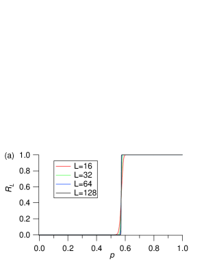
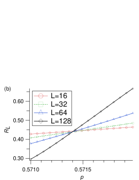
Figure 4: (a) Wrapping probability $R_{L}$ vs. occupation probability $p$ for sites on the (10,3)-a lattice. The curves for different system sizes $L$ cross around $p_{c}\approx 0.5714$. (b) Zoom of previous plot.

III.2 The uncertainty in the percolation threshold

There is an easy way to determine the uncertainty in $p_{c}$ based only on the simulation output, and without any assumptions about critical exponents. In a plot of $R_{L}(p)$, the percolation transition is identified by looking for a value of $p$ at which the wrapping probability is approximately stationary as the system size changes. However, the wrapping probabilities are determined from finite samples in Monte Carlo simulations, and (as described below) this gives rise to statistical fluctuations in $R_{L}$ for all $p$ values. A fluctuation $\delta R_{L}$ shifts the curve along the horizontal axis by an amount $\delta R_{L}/(dR_{L}/dp)$, where $dR_{L}/dp$ is the slope of the $R_{L}$ vs. $p$ curve.

In order to get the uncertainty in $R_{L}(p)$, let us first consider $R_{L}$ as a function of occupation number $n$ rather than occupation probability $p$. We use generate $N_{L}$ lattices with $n$ occupied sites, and use the Newman-Ziff algorithm to determine the number $N_{L}*R_{L}(n)$ that wrap. If we were to do this process repeatedly, we would find that the number wrapping obeys a binomial distribution with mean $N_{L}R_{L}(n)$ and variance $N_{L}R_{L}(n)(1-R_{L}(n))$, and so the fraction $R_{L}(n)$ that wrap has mean $R_{L}(n)$ and variance $R_{L}(n)(1-R_{L}(n))/N_{L}$.

When we go from $R_{L}(n)$ to $R_{L}(p)$, the convolution with a binomial distribution means that $R_{L}(p)$ is a weighted sum of different $R_{L}(n)$ values. However, $R_{L}(n+1)$ is not statistically independent of $R_{L}(n)$, since it is generated by occupying one more site (or bond) in each of the lattices used to determine $R_{L}(n)$. Near $p_{c}$, $R_{L}(n\neq Np_{c})$ is approximately a linear function of $n-Np_{c}$:

$$R_{L}(n)\approx R_{L}(Np_{c})+c*(n-Np_{c})+\eta(n)$$ (4)

where $c$ is an unknown constant and $\eta$ is a noise term.

This expression for $R_{L}(n)$ is convolved with a binomial probability distribution that is approximately Gaussian for large $N$ (and hence even about $p_{c}$). The normalization of the probability distribution means that the convolution with the first term gives $R_{L}(Np_{c})$. The symmetry of the peak of the distribution means that the convolutions with the second and third terms vanish. We thus conclude that $R_{L}(p=p_{c})\approx R_{L}(n=Np_{c})$, and so we will use $\sqrt{\frac{R_{L}(1-R_{L})}{N_{L}}}$ for the uncertainty in $R_{L}(p_{c})$. This, in turn gives the uncertainty in $p_{c}$ as:

$$\delta p_{c}=\sqrt{\frac{R_{L}(1-R_{L})}{N_{L}}}\left/\frac{dR_{L}}{dp}\right.$$ (5)

We have neglected the variance of the weighted sum of the noise terms $\eta(n)$ in Eq. (4), but that variance is small because $\eta(n)$ exhibits correlations for nearby $n$ values: The fact that $R_{L}(n)$ is an increasing function of $n$ means that downward fluctuations of $R_{L}(n)$ are limited in magnitude by the fluctuations of $R_{L}(n-1)$. The fact that $R_{L}\leq 1$ reduces the probability of successive upward fluctuations.

In Eq. (5), we use the slope of the steepest $R_{L}$ vs. $p$ curve. If the steepest curve were perfectly vertical, fluctuations of the other curves would be completely irrelevant, and the point of intersection would remain on that curve at the value of $p$ where it rises. Consequently, the finite slope of the steepest curve is the limiting factor in our determination of $p_{c}$.

IV Results

Figures 5 through 7 show $R_{L}$ vs. $L$ (for different $p$ values), for site and bond percolation on the lattices under study. The number of unit cells in a realization of each lattice is $L^{3}$, so that the number of lattice sites is $4L^{3}$ (for the (10,3)-a and (10,3)-b lattices) or $6L^{3}$ (for (8,3)-a). The number of bonds is $6L^{3}$ (for (10,3)-a and (10,3)-b) or $9L^{3}$ (for (8,3)-a). In all plots, site occupation probability $p$ was incremented in steps of $1/\text{number of sites or bonds for smallest $L$ value}$.

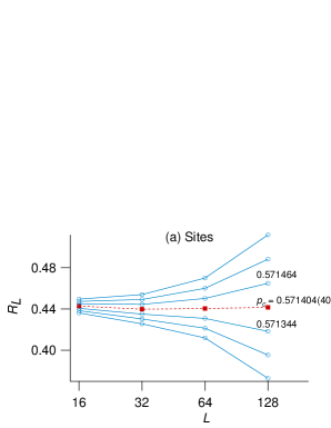
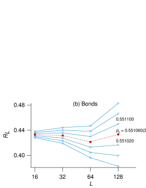
Figure 5: Wrapping probability $R_{L}$ vs. $L$ for (a) site and (b) bond percolation on (10,3)-a lattices, for different occupation probabilities $p$. (Selected $p$ values shown to right of plots.) The percolation threshold $p_{c}$ is the value of $p$ that gives the flattest overall trend. The uncertainty is determined via Eq. (5).

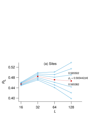
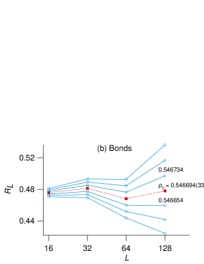
Figure 6: Wrapping probability $R_{L}$ vs. $L$ for (a) site and (b) bond percolation on (10,3)-b lattices, for different occupation probabilities $p$. (Selected $p$ values shown to right of plots.) The percolation threshold $p_{c}$ is the value of $p$ that gives the flattest overall trend. The uncertainty is determined via Eq. (5).

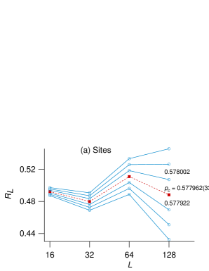
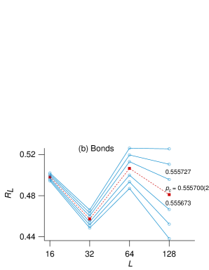
Figure 7: Wrapping probability $R_{L}$ vs. $L$ for (a) site and (b) bond percolation on (8,3)-a lattices, for different occupation probabilities $p$. (Selected $p$ values shown to right of plots.) Although there is some oscillation, the percolation threshold $p_{c}$ is the value of $p$ that gives the flattest overall trend. The uncertainty is determined via Eq. (5).

Table 1: Site and bond percolation thresholds for important 3-dimensional lattices with different coordination numbers $z$. Uncertainties are given in parentheses, and refer to the last one or two digits, depending on the number of digits in the uncertainty. Bibliographic references are in brackets [].

lattice	$z$	$p_{c}$ (site)	$p_{c}$ (bond)
(8,3)-a	3	$0.577962(33)$	$0.555700(22)$
(10,3)-a	3	$0.571404(40)$	$0.551060(37)$
(10,3)-b	3	$0.565442(40)$	$0.546694(33)$
diamond	4	$0.4301(4)$Van Der Marck (1998)	$0.3893(2)$Van Der Marck (1998)
simple cubic	6	$0.3116080(4)$Lorenz and Ziff (1998a)	$0.2488126(5)$Lorenz and Ziff (1998b)
bcc	8	$0.2459615(10)$Lorenz and Ziff (1998a)	$0.1802875(10)$Lorenz and Ziff (1998b)
fcc	12	$0.1992365(10)$Lorenz and Ziff (1998b)	$0.1201635(10)$Lorenz and Ziff (1998a)
hcp	12	$0.1992555(10)$Lorenz et al. (2000)	$0.1201640(10)$Lorenz et al. (2000)

V Discussion

The percolation thresholds identified for the 3-coordinated lattices considered here are higher than typical values for 3-dimensional lattices that have been studied previously. This point is illustrated in Table 1, which shows percolation thresholds for a variety of common 3-dimensional lattices, organized by their coordination number $z$. It is clear from the table that $p_{c}$ increases as $z$ decreases. This makes intuitive sense: With lower coordination numbers, it is easier to destroy a spanning cluster by removing a few sites or bonds at key points, while in lattices with higher coordination numbers there are more paths that can be navigated to circumvent a missing site or bond.

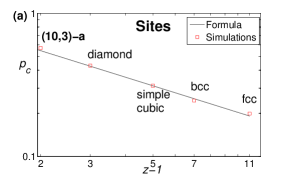
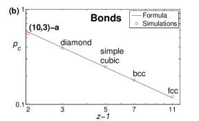
Figure 8: A log-log plot of computationally-determined site (top) and bond (bottom) percolation thresholds vs. $(z-1)$ for different 3D lattices, and a comparison plot of the formula of Galam and MaugerGalam and Mauger (1996). Simulation values for (10,3)-a are from Fig. 5. Simulations values for the other lattices are from the references in Table 1.

The information shown in Table 1 can be compared with an analytical expressionGalam and Mauger (1996) for the approximate dependence of $p_{c}$ on spatial dimension $d$ and coordination number $z$:

$$p_{c}=p_{0}\left((d-1)(z-1)\right)^{-a}d^{b}$$ (6)

where $a=0.6160$ for sites and 0.9346 bonds, $b=0$ for sites and $b=a$ for bonds, and $p_{0}=1.2868$ for sites and 0.7541 for bonds. This comparison is done in Fig. 8. For ease of presentation we only show the (10,3)-a lattice on these plots, but the percolation thresholds of the other 3-connected lattices differ by only about $1\%$, and would overlap the (10,3)-a lattice if included. Crucially, the percolation thresholds of the 3-connected lattices are very close to the theoretical plot.

We have not explored the entire family of 3-connected nets studied by Wells. Thus, it is an open question as to whether there are simple 3-dimensional periodic lattices with higher percolation thresholds. We qualify the previous sentence with the word “simple” because it is intuitively obvious that one could often trivially increase the percolation threshold of a crystalline structure by inserting chains of 2-connected sites between sites with higher coordination numbers. The interesting question is whether one can construct crystals with higher $p_{c}$ without making use of 2-connected sites between higher-coordinated cites.

In conclusion, we have used Monte Carlo simulations to determine the percolation thresholds of several interesting lattices that have not, to the best of our knowledge, been studied previously. We find that these lattices have substantially higher percolation thresholds than other 3-dimensional lattices, due to their low coordination numbers. The results for both bond and percolation thresholds are very close to theoretical predictions that rely on coordination number and dimensionality.