A hybrid HDMR for mixed multiscale finite element methods with application to flows in random porous media

Abstract

Stochastic modeling has become a popular approach to quantify uncertainty in flows through heterogeneous porous media. In this approach the uncertainty in the heterogeneous structure of material properties is often parametrized by a high-dimensional random variable, leading to a family of deterministic models. The numerical treatment of this stochastic model becomes very challenging as the dimension of the parameter space increases. To efficiently tackle the high-dimensionality, we propose a hybrid high-dimensional model representation (HDMR) technique, through which the high-dimensional stochastic model is decomposed into a moderate-dimensional stochastic model in the most active random subspace, and a few one-dimensional stochastic models. The derived low-dimensional stochastic models are solved by incorporating the sparse-grid stochastic collocation method with the proposed hybrid HDMR. In addition, the properties of porous media, such as permeability, often display heterogeneous structure across multiple spatial scales. To treat this heterogeneity we use a mixed multiscale finite element method (MMsFEM). To capture the non-local spatial features (i.e. channelized structures) of the porous media and the important effects of random variables, we can hierarchically incorporate the global information individually from each of the random parameters. This significantly enhances the accuracy of the multiscale simulation. Thus, the synergy of the hybrid HDMR and the MMsFEM reduces the dimension of the flow model in both the stochastic and physical spaces, and hence, significantly decreases the computational complexity. We analyze the proposed hybrid HDMR technique and the derived stochastic MMsFEM. Numerical experiments are carried out for two-phase flows in random porous media to demonstrate the efficiency and accuracy of the proposed hybrid HDMR with MMsFEM.

1 Introduction

The modeling of dynamic flow and transport processes in geologic porous media plays a significant role in the management of natural resources, such as oil reservoirs and water aquifers. These porous media are often created by complex geological processes and may contain materials with widely varying abilities to transmit fluids. Thus, multiscale phenomena are inherent in these applications and must be captured accurately in the model. In addition, due to measurement errors and limited knowledge of the material properties and external forcing, modeling of subsurface flow and transport often uses random fields to represent model inputs (e.g., permeability). Then the system’s behavior can be accurately predicted by efficiently simulating the stochastic multiscale model. The existence of heterogeneity at multiple scales combined with this uncertainty brings significant challenges to the development of efficient algorithms for the simulation of the dynamic processes in random porous media. As a result, the interest in developing stochastic multiscale methods for stochastic subsurface models has steadily grown in recent years.

The existence of uncertainty in random porous media is an important challenge for simulations. One way to describe the uncertainty is to model the random porous media as a random field which satisfies certain statistical correlations. This naturally results in describing the flow and transport problem using stochastic partial differential equations (SPDE). Over the last few decades several numerical methods have been developed for solving SPDEs. The existing stochastic numerical approaches roughly fall into two classes: (1) non-intrusive schemes and (2) intrusive schemes. In non-intrusive schemes, the existing deterministic solvers are used without any modification to solve a (large) set of deterministic problems, which correspond to a set of samples from the random space. This leads to a set of outputs, which are used to recover the desired statistical quantities. Monte Carlo methods [14] and stochastic collocation methods fall into this category. In contrast, intrusive schemes treat the approximation of the probabilistic dependence directly in the SPDE. Thus, discretization leads to a coupled set of equations that are fundamentally different from discretizations of the original deterministic model, and hence, raises new challenges for nonlinear solvers. Typical examples from this class are stochastic Galerkin [19, 13, 34] and perturbation methods [48]. A broad survey of these methods can be found in [29]. Among these methods, stochastic collocation methods have gained significant attention in the research community because they share the fast convergence property of the stochastic finite element methods while having the decoupled nature of Monte Carlo methods. A stochastic collocation method consists of two components: a set of collocation points and an interpolation operator. The collocation points are selected based on specific objectives, and choosing different objectives or constraints leads to different methods. Two popular collocation methods are the full-tensor product method [5] and the Smolyak sparse-grid method [6, 36, 40]. Sparse-grid stochastic collocation is known to have the same asymptotic accuracy as full-tensor product collocation, but uses significantly fewer collocation points. Unfortunately, the number of collocation points required in the sparse-grid method still increases dramatically for high-dimensional stochastic problems. Hence, application of this method is still limited to problems in a moderate-dimensional stochastic space.

Due to small correlation lengths in the covariance structure, the uncertainty in characterizations of porous media are often parametrized by a large number of random variables, e.g., using a truncated Fourier type expansion for random fields. Consequently, the model’s input is defined in a high-dimensional random parameter space. Sampling in high-dimensional random spaces is computationally demanding and very time-consuming. If the sampling of random space is conducted in the full random space through the stochastic collocation method, then the number of samples increases sharply with respect to the dimension of the random space. This is the notorious curse of dimensionality, and is a fundamental problem facing stochastic approximations in high-dimensional stochastic spaces. Dimension reduction techniques such as proper orthogonal decomposition, principal component analysis, reduced basis methods [39], novel random field expansion techniques [27, 45, 46] and high-dimensional model representations (HDMRs) [38], strive to address this problem. Among these methods, the HDMR is one of the most promising methods for efficient stochastic dimension reduction in subsurface applications, and has received considerable attention in recent years [32, 33, 35, 47]. The HDMR was originally developed in the application of chemical models by [38], but was later cast as a general set of quantitative assessment and analysis tools for capturing the high-dimensional relationship between model inputs and model outputs. HDMR has been used for improving the efficiency of deducing high-dimensional input-output system behavior, and can be employed to reduce the computational effort. In practice, to avoid dealing with the full high-dimensional random space, a truncated HDMR technique is used to decompose a high-dimensional model into a set of low-dimensional models, each of which needs much less computational effort. The curse of dimensionality can be suppressed significantly by using this approach to HDMR. However, some drawbacks exist in the traditional truncated HDMR [9, 38] and related methods such as the adaptive HDMR [32, 47]. For example, often too many low-dimensional models need to be computed, and high-order cooperative effects from important random variables may be neglected. To overcome these drawbacks, we propose a hybrid HDMR, which implicitly uses the complete HDMR in a moderate-dimensional space and explicitly uses the first-order truncated HDMR for the remaining dimensions. Thus the hybrid HDMR decomposes a high-dimensional model into a moderate-dimensional model and a few one-dimensional models. The moderate-dimensional space is spanned by the most active random dimensions. We use sensitivity analysis to identify the most active random dimensions. Then each low-dimensional stochastic model in the hybrid HDMR is solved by using sparse-grid stochastic collocation method. The proposed hybrid HDMR renders a good approximation in stochastic space and substantially improves the efficiency for high-dimensional stochastic models. Therefore, a good trade-off between computational complexity and dimension reduction error can be achieved with the hybrid HDMR technique.

Porous media often exhibit complex heterogeneous structures that are inherently hierarchical and multiscale in nature, and hence, pose a significant challenge for developing accurate and efficient numerical methods. Simulating flow in porous media using a very fine grid to resolve this heterogeneous structure is computationally very expensive and possibly infeasible. However, disregarding the heterogeneities can lead to large errors. Thus, many multiscale methods including the MMsFEM [7], variational multiscale method [23], two-scale conservative subgrid approaches [3] and heterogeneous multiscale method [10], multiscale finite volume method [24], spectral MsFEM [11] (see [12] for more complete references), have been developed over the last few decades to capture the influence of fine- and multi-scale heterogeneities in under-resolved simulations. We note that these multiscale methods share some similarities [12]. In this paper, we focus on the MMsFEM. The main idea behind MMsFEM is to incorporate fine-scale information into the finite element velocity basis functions, and hence, capture the influence of these fine scales in a large-scale mixed finite element formulation. The MMsFEM retains local conservation of velocity flux and has been shown to be effective for solving flow and transport equations in heterogeneous porous media. In many cases, the overhead of computing multiscale basis functions can be amortized as they can be computed once for a particular medium, and then reused in subsequent computations with different source terms and boundary conditions. This leads to a large computational savings in simulating the flow and transport process where the flow equation needs to be solved many times dynamically. When porous media exhibit non-separable scales, some global information is needed to represent non-local effects (e.g., channel, fracture and shale barriers) and is used to construct the multiscale basis functions. Using global information can significantly improve the simulation accuracy in these important geological settings [1, 2, 25, 26]. If the global information is incorporated into MMsFEM, we refer to the MMsFEM as global MMsFEM (G-MMsFEM). In the paper, we extend the central concept of the global information to MMsFEM based on the hybrid HDMR.

Combining different multiscale methods and stochastic numerical approaches yields various stochastic multiscale methods [15, 16, 20, 26, 27, 33, 44]. These methods established a general approach to solve problems in multiscale stochastic media. Specifically, dimension reduction techniques are applied, particularly focusing on the multiscale spatial dimension of these stochastic models, to reduce the overall computational cost. For example, within the stochastic Galerkin framework several earlier works (e.g., [4, 35, 39]) proposed solving an optimization problem to select a set of optimal basis functions to define a reduced model. Although, these approaches reduce the resolution of the spatial dimension, the stochastic dimension is not reduced. Therefore, the computational cost of these approaches may still be too expensive in high-dimensional stochastic spaces.

In this paper, we propose a hybrid HDMR framework, and use the sparse-grid stochastic collocation method with MMsFEM to develop a reduced multiscale stochastic model. Sensitivity analysis is used to control the reduction of the stochastic dimension. For the MMsFEM, we hierarchically utilize approximate global information that is aligned with the terms of the hybrid HDMR. Specifically, only the required basis functions are computed and to amortize their computational cost they are held constant in time. Thus, the proposed multiscale stochastic model reduction approach is able to reduce a high-dimensional stochastic multiscale model in both stochastic space, and the resolution of physical space. Compared with traditional truncated HDMR techniques, much better efficiency and very good accuracy are achieved with this hybrid HDMR. We analyze the proposed multiscale stochastic model reduction approach and investigate its application to flows in random and heterogeneous porous media. Important statistical properties (e.g., mean and variance) of the outputs of the stochastic flow models are computed and discussed.

The rest of the paper is organized as follows. In Section $2$, we briefly introduce the background on the flow and transport models in random porous media. In Section $3$, we present a general framework for HDMR and propose the hybrid HDMR technique. Some theoretical results and computational complexity are also addressed in this section. Section $4$ is devoted to presenting MMsFEM integration with the hybrid HDMR. In Section $5$, numerical examples using two-phase flow are presented to demonstrate the performance of the proposed the hybrid HDMR with MMsFEM. Finally, some conclusions and closing remarks are made.

2 Background and notations

2.1 Two-phase flow system and its stochastic parametrization

Let $D$ be a convex bounded domain in $\mathbb{R}^{d}$ ($d=2,3$) and $(\Omega,F,P)$ be a probability space, where $\Omega$ is the set of outcomes, $F$ is the $\sigma$-algebra generated by $\Omega$, and $P$ is a probability measure.

We consider two-phase flow and transport in a random permeability field, $k(x,\omega)$. Here the two phases are referred to as water and oil, and designated by subscripts $w$ and $o$, respectively. The equations of two-phase flow and transport (in the absence of gravity and capillary effects) can be written:

$$-div(\lambda(S){k(x,\omega)}\nabla p) =q,$$ (1)

$${\partial S\over\partial t}+div(uf_{w}(S)) =0,$$ (2)

where the total mobility $\lambda(S)$ is given by $\lambda(S)=\lambda_{w}(S)+\lambda_{o}(S)$ and $q$ is a source term. Here $\lambda_{w}(S)=k_{rw}(S)/\mu_{w}$ and $\lambda_{o}(S)=k_{ro}(S)/\mu_{o}$, where $\mu_{o}$ and $\mu_{w}$ are viscosities of oil and water phases, respectively, and $k_{rw}(S)$ and $k_{ro}(S)$ are relative permeabilities of oil and water phases, respectively. Here $f_{w}(S)$ is the fractional flow of water and given by $f_{w}=\lambda_{w}/(\lambda_{w}+\lambda_{o})$, Equation (1) is the flow equation governing the water pressure, and (2) is the transport (or saturation) equation. According to Darcy’s law, the total velocity $u$ in (2) is given by

$$u=u_{w}+u_{o}=-\lambda(S){k}\nabla p.$$ (3)

A random field may be parameterized by a Fourier type expansion, such as the expansion of Karhunen-Loève (ref.[31]), polynomial chaos or wavelet [29]. This often gives rise to an infinite-dimensional random space. For computation, we truncate such an expansion to approximate the random field. Then $k(x,\omega)$ can be formally described by

$$k(x,\omega)\approx k\big{(}x,\theta_{1}(\omega),\theta_{2}(\omega),\dots,\theta_{N}(\omega)\big{)}.$$ (4)

For example, if a random field is characterized by a covariance structure, then the random field can be approximated by a finite sum of uncorrelated random variables through a truncated Karhunen-Loève expansion (KLE). To obtain an accurate approximation, a large number $N$ of random parameters is required in (4). This leads to a family of deterministic models in a high-dimensional random parameter space.

To simplify the presentation, we make the following assumption,

$$k(x,\omega)=k(x,\Theta),\quad\text{ where $\Theta:=\Theta(\omega)=\big{(}\theta(\omega_{1}),\theta_{2}(\omega),\dots,\theta_{N}(\omega)\big{)}\in\mathbb{R}^{N}$}.$$

Let $I^{N}\subset\mathbb{R}^{N}$ be the image of $\Theta$, i.e., $I^{N}=\Theta(\Omega)$, and $\rho(\Theta)=\Pi_{i=1}^{N}\rho_{i}(\theta_{i})$ be the joint probability function of $(\theta_{1},\cdots,\theta_{N})$. By equations (1), (2), (3) and parametrization of permeability field, we formulate the following stochastic two-phase flow system: Find random fields $p(x,\Theta,t)$, $v(x,\Theta,t)$, $S(x,\Theta,t):D\times I^{N}\times(0,T]\longrightarrow\mathbb{R}$ such that they almost surely (a.s) satisfy the following equations subject to initial and boundary conditions,

$$\begin{split}\begin{cases}&\mbox{div}(u)=q\\ &u=-\lambda(S)k(x,\Theta)\nabla p\\ &\displaystyle\frac{\partial S}{\partial t}+\mbox{div}\big{(}uf_{w}(S)\big{)}=0.\\ \end{cases}\end{split}$$ (5)

To further simply the notation, we will suppress the spatial variable $x$ and temporal variable $t$ in the rest of paper when no ambiguity occurs.

2.2 Sparse grid stochastic collocation method

For stochastic two-phase flow systems (5), the statistical properties (e.g., mean and variance) of solutions are of interest. These properties may be obtained by first sampling the parameter random space using, for example, a Monte Carlo method or sparse grid collocation method, then solving the deterministic problems for the samples and analyzing the corresponding results to obtain the desired statistical quantities. The convergence of Monte Carlo methods is slow and a very large number of samples may be required, which leads to high computational cost. Instead, we use the Smolyak sparse-grid collocation method [40], where the Smolyak interpolant $\mathcal{A}(N+\ell,N)$ ($\ell\geq 1$) is a linear combination of tensor product interpolants with the property: only products with a relatively small number of nodes are used and the linear combination is chosen in such a way that an interpolation property for $N=1$ is preserved for $N>1$ [6]. In the notation $\mathcal{A}(N+\ell,N)$, the $\ell$ represents the interpolation level. The sparse-grid collocation method is known to have the same asymptotic accuracy as tensor product collocation method, while requiring many fewer collocation points as the parameter dimension increases [36].

Sparse grids have been successfully applied to stochastic collocation in many recent works (e.g., [32, 33, 26]). Based on Smolyak formula (ref.[6]), a set of collocation points $\{\Theta^{(j)}\}_{j=1}^{N_{c}}$ in $I^{N}$ are specially chosen, where $N_{c}$ is the number of collocation points. With these chosen collocation points and corresponding weights $\{w^{(j)}\}_{j=1}^{N_{c}}$, the statistical properties of the solutions can be obtained. At each of the collocation points, the deterministic system (5) is solved and the output, for example, $S(x,\Theta^{(j)},t)$ is obtained. Then the mean of $S(x,\Theta,t)$ can be estimated by

$$E[S(x,\Theta,t)] = \int_{I^{N}}S(x,\Theta,t)\rho(\Theta)d\Theta$$

$$\approx \int_{I^{N}}\mathcal{A}(N+\ell,N)\big{[}S(x,\Theta,t)\big{]}\rho(\Theta)d\Theta=\sum_{j=1}^{N_{c}}S(x,\Theta^{(j)},t)w^{(j)}.$$

Here the weights $\{w^{(j)}\}_{j=1}^{N_{c}}$ are determined by the basis functions of $\mathcal{A}(N+\ell,N)$ and joint probability function $\rho(\Theta)$ (ref.[18]). Similarly, the variance of $S(x,\Theta^{(j)},t)$ can be obtained by

$$\begin{split}\mbox{Var}[S(x,\Theta,t)]&=&\int_{I^{N}}\big{(}S(x,\Theta,t)-E[S(x,\Theta,t)]\big{)}^{2}\rho(\Theta)d\Theta\\ &\approx&\sum_{j=1}^{N_{c}}S^{2}(x,\Theta^{(j)},t)w^{(j)}-E^{2}[S(x,\Theta,t)].\end{split}$$ (6)

Let $H(N+\ell,N)$ denote the number of collocation points for Smolyak sparse grid interpolation $\mathcal{A}(N+\ell,N)$. Then it follows that (see [6])

$$H(N+\ell,N)\approx\frac{2^{\ell}}{\ell!}N^{\ell}\quad\text{for $N\gg 1$}.$$ (7)

This implies that the number of collocation points algebraically increases with respect to the dimension $N$. We utilize Smolyak sparse grid collocation for the numerical computation. The stochastic approximation of the Smolyak sparse grid collocation method depends on the number of collocation points and the dimension $N$ of the random parameter space. The convergence analysis in [36] implies that the convergence of Smolyak sparse grid collocation is exponential with respect to the number of Smolyak points, but depends on the parameter dimension $N$. This exponential convergence rate behaves algebraically for $N\gg 1$.

3 High dimensional model representation

The truncated KLE leads to the family of two-phase flow deterministic models (5) with a high-dimensional parameter $\Theta$. The most challenging part of solving such a high-dimensional stochastic system is to discretize the high-dimensional stochastic space. There exist a few methods for the discretization of the random space [4, 6, 5, 13, 14, 16, 19, 29, 33, 35, 36, 42, 48] (more references can be found therein). Among these methods, the sparse-grid collocation method has been widely used and generates completely decoupled systems, each of which is the same size as the deterministic system. This method is usually very efficient in moderate-dimensional spaces. However, when the dimension of the random parameter is large, a large number of collocation points are required (7), and the deterministic model (5) must be solved at each of these collocation points. Consequently, the efficiency of this collocation method will deteriorate in a high-dimensional space. To overcome this difficulty, we use a high-dimensional model representation (HDMR) to reduce the stochastic dimension and enhance the efficiency of the simulation. By truncating HDMR, the high-dimensional model can be decomposed into a set of low-dimensional models. Hence the computational effort can be significantly reduced [32, 47].

In the following section, we present a general HDMR framework and propose a hybrid HDMR method.

3.1 A general HDMR framework

In this section, we adopt the decomposition of multivariate functions described in [28] to present a general HDMR framework in terms of operator theory. Let $\mathcal{F}$ be a linear space of real-valued functions $f(\Theta)$ defined on a cube $I^{N}$ and $\Theta:=(\theta_{1},\theta_{2},\cdots,\theta_{N})\in I^{N}$. In this discussion $f(\Theta)$ represents a relationship between the random vector model input, $\Theta$, and a model output (e.g., saturation, water-cut).

To introduce HDMR approach, we define a set of projection operators as follows.

Definition 1.

[28] Let $\{\mathrm{P_{j}}\}_{j=1}^{N}$ be a set of commuting projection operators on $\mathcal{F}$ satisfying the following property:

$$\mathrm{P_{j}}(f)=f\quad\text{if $f$ does not depend on $\theta_{j}$, and $\mathrm{P_{j}}(f)$ does not depend on $\theta_{j}$}.$$ (8)

Let $\mathbf{u}\subseteq\{1,\cdots,N\}$ be a subset and $I$ the identity operator, we define

$$\mathrm{P}_{\mathbf{u}}:=\Pi_{j\in\mathbf{u}}\mathrm{P_{j}},\quad\text{and}\quad\mathrm{P}_{\emptyset}:=I.$$

Associated with projection $\mathrm{P}_{\mathbf{u}}$, we define $\widehat{\mathrm{P}}_{\mathbf{u}}:=\mathrm{P}_{\{1,\cdots,N\}\setminus\mathbf{u}}$. Then $\widehat{\mathrm{P}}_{\mathbf{u}}f$ only depends on the variables with indices in $\mathbf{u}$.

Let $\mu$ be a measure on Borel subsets of $I^{N}$ and a product measure with unit mass, i.e.,

$$d\mu(\Theta):=\Pi_{i=1}^{N}d\mu_{i}(\theta_{i}),\quad\int_{I}d\mu_{i}(\theta_{i})=1,\quad i=1,\cdots,N.$$ (9)

The inner product $\langle\cdot,\cdot\rangle$ on $\mathcal{F}$ induced by the measure $\mu$ is defined as follows:

$$\langle f,h\rangle:=\int_{I^{N}}f(\Theta)h(\Theta)d\mu(\Theta),\quad f,g\in\mathcal{F}.$$

The norm $\|\cdot\|_{\mathcal{F}}$ on $\mathcal{F}$ is defined by $\|f\|_{\mathcal{F}}:=\langle f,f\rangle^{1/2}$. Given the measure $\mu$, we can specify the projection operator in (8). We assume that the functions in $\mathcal{F}$ are integrable with respect to $\mu$. For any $f\in\mathcal{F}$ and $j\in\{1,\cdots,N\}$, we define

$$\mathrm{P}_{j}f(\Theta)=\int_{I}f(\Theta)d\mu_{j}(\theta_{j}).$$ (10)

Consequently, $\widehat{\mathrm{P}}_{\mathbf{u}}f(\Theta)=\int_{I^{N-|\mathbf{u}|}}f(\Theta)\Pi_{j\notin\mathbf{u}}d\mu_{j}(\theta_{j})$ for any $\mathbf{u}\subseteq\{1,\cdots,N\}$. By the definitions of these projection operator, we can obtain a decomposition of $\mathcal{F}$ as following (see [37]),

$$\mathcal{F}=\oplus_{\mathbf{u}\subseteq\{1,\cdots,N\}}\mathcal{F}_{\mathbf{u}},\quad\text{where}\quad\mathcal{F}_{\mathbf{u}}=\bigg{(}\Pi_{j\in\mathbf{u}}(I-\mathrm{P}_{j})\bigg{)}\widehat{\mathrm{P}}_{\mathbf{u}}\mathcal{F}.$$ (11)

For any $\mathbf{u}\subseteq\{1,\cdots,N\}$, we define

$$\mathrm{M}_{\mathbf{u}}=\bigg{(}\Pi_{j\in\mathbf{u}}(I-\mathrm{P}_{j})\bigg{)}\widehat{\mathrm{P}}_{\mathbf{u}}.$$

Then we can show the operators $\mathrm{M}_{\mathbf{u}}$ are commutative projection operators and mutually orthogonal, i.e.,

$$\mathrm{M}_{\mathbf{u}}^{2}=\mathrm{M}_{\mathbf{u}},\quad\mathrm{M}_{\mathbf{u}}\mathrm{M}_{\mathbf{v}}=0\quad\text{for $\mathbf{u}\neq\mathbf{v}$}.$$

The equation (11) gives an abstract HDMR expansion of $f$ by

$$f=\sum_{\mathbf{u}\subseteq\{1,\cdots,N\}}f_{\mathbf{u}}=\sum_{\mathbf{u}\subseteq\{1,\cdots,N\}}\mathrm{M}_{\mathbf{u}}f,\quad\text{where $\mathrm{M}_{\mathbf{u}}f\in\mathcal{F}_{\mathbf{u}}$}.$$ (12)

The equation (11) also implies that

$$\|f\|^{2}_{\mathcal{F}}=\sum_{\mathbf{u}\subseteq\{1,\cdots,N\}}\|\mathrm{M}_{\mathbf{u}}f\|_{\mathcal{F}}^{2},\quad\widehat{\mathrm{P}}_{\emptyset}(\mathrm{M}_{\mathbf{u}}f)=0\quad\text{for $\mathbf{u}\neq\emptyset$}.$$

Any set of commutative projectors $\{\mathrm{M}_{\mathbf{v}}\}$ generate a distributive lattice whose elements are obtained by all possible combinations (addition and multiplication) of the projectors in the set. The lattice has a unique maximal projection operator $\mathcal{M}$, which gives the algebraically best approximation to the functions in $\mathcal{F}$ [21]. The range of the maximal projection operator $\mathcal{M}$ for the lattice is the union of the ranges of $\{\mathrm{M}_{\mathbf{v}}\}$. Because the commutative projectors $\{\mathrm{M}_{\mathbf{v}}\}$ are mutually orthogonal here, the maximal projection operator $\mathcal{M}$ and the range $\mathcal{F}_{\mathcal{M}}$ of $\mathcal{M}$ have explicit expressions as follows:

$$\mathcal{M}=\sum_{\mathbf{v}}\mathrm{M}_{\mathbf{v}},\quad\mathcal{F}_{\mathcal{M}}=\oplus_{\mathbf{v}}\mathcal{F}_{\mathbf{v}}.$$

As more orthogonal projectors are retained in the set, the resulting approximation by the maximal projection operator $\mathcal{M}$ will become better.

If the measure $\mu$ in (9) is taken to be the probability measure

$$d\mu(\Theta)=\rho(\Theta)d\Theta=\Pi_{i=1}^{N}\rho_{i}(\theta_{i})d\theta_{i},$$

then the resulting HDMR defined in (12) is called ANOVA-HDMR [38] . Let us fix a point $\overline{\Theta}:=(\bar{\theta}_{1},\bar{\theta}_{2},\cdots,\bar{\theta}_{N})$. If the measure $\mu$ in (9) is taken as the Dirac measure located at the point $\Theta$, i.e.,

$$d\mu(\Theta)=\Pi_{i=1}^{N}\delta(\theta_{i}-\bar{\theta}_{i})d\theta_{i},$$

then the resulting HDMR is Cut-HDMR. The point $\overline{\Theta}$ is so called cut-point or anchor point. In ANOVA-HDMR, the $\widehat{\mathrm{P}}_{\mathbf{v}}f$ involves $N-|\mathbf{v}|$ dimensional integration and the computation of the components of $f$ is expensive. In Cut-HDMR, the $\widehat{\mathrm{P}}_{\mathbf{v}}f$ only involves the evaluation in a $N-|\mathbf{v}|$ dimensional space and the computation is cheap and straightforward. Because of this reason, we use Cut-HDMR for the analysis and computation in the paper.

3.2 A hybrid HDMR

In this subsection, we use a less abstract representation of the HDMR to motivate approximations suitable for practical computation. Specifically, we review the traditional approach to truncated HDMR, and then propose and analyze an alternative hybrid HDMR.

Expanding elements of (12), the HDMR of $f(\Theta)$ can be written in the form,

$$f(\Theta)=f_{0}+\sum_{i=1}^{n}f_{i}(\theta_{i})+\sum_{i<j}f_{ij}(\theta_{i},\theta_{j})+\cdots f_{12\cdots n}(\theta_{1},\theta_{2},\cdots,\theta_{n}).$$ (13)

Here $f_{0}$ is the zeroth-order component denoting the mean effect of $f(\Theta)$. The first-order component $f_{i}(\theta_{i})$ represents the individual contribution of the input $\theta_{i}$ and the second-order component $f_{ij}(\theta_{i},\theta_{j})$ represents the cooperative effects of $\theta_{i}$ and $\theta_{j}$ and so on. We define $q$-th order truncated HDMR by

$$\mathcal{M}_{q}f=f_{0}+\sum_{m=1}^{q}\sum_{i_{1}<\cdots i_{m}}f_{i_{1}\cdots i_{m}}(\theta_{i_{1}}\cdots\theta_{i_{m}}).$$ (14)

For most realistic physical systems, low-order HDMR $\mathcal{M}_{q}f$ (e.g., $q\leq 3$) may give a good approximation [38]. The $\mathcal{M}_{q}f$ can approximate $f(\Theta)$ through truncating the HDMR. The $\mathcal{M}_{q}f$ consists of a large number of component terms for high-dimensional models, the computation of all the components may be costly. For many cases, some high-order cooperative effects cannot be neglected in the model’s output, especially when a model strongly relies on a few dependent variables. Consequently, the traditional truncated HDMR in (14) may not yield a very good approximation. To eliminate or alleviate these drawbacks of traditional truncated HDMR, we propose a new truncated HDMR, which we refer to as hybrid HDMR.

We use the Fourier amplitude sensitivity test [9] to select the most active dimensions from the components of the high-dimensional random vector $\Theta$. Let $\{f_{j}\}_{j=1}^{N}$ be the first-order components defined in Eq.(13) and let $\sigma^{2}(f_{j})$ denote the variance of $f_{j}$. We may assume that $\sigma^{2}(f_{1})\geq\sigma^{2}(f_{2})\geq\cdots\geq\sigma^{2}(f_{N})$ as we can re-order the index set $\{j\}_{j=1}^{N}$ to satisfy this requirement. Alternatively, we can order the index set to produce monotonically decreasing expectations, $E[f_{1}]\geq E[f_{2}]\geq\cdots\geq E[f_{N}]$, and use this ordering to select the most active dimensions. In this paper, we only consider the variance sensitivity, and we calculate $\sigma^{2}(f_{i})$ ($i=1,\cdots N$) using the method described in (6). Because the first-order components $\{f_{i}\}_{i=1}^{N}$ are defined in one-dimensional random parameter spaces, the computational cost for $\{\sigma^{2}(f_{i})\}_{i=1}^{N}$ is very small. Moreover, most of the elements in $\{\sigma^{2}(f_{i})\}_{i=1}^{N}$ will be reused when we calculate the variance of outputs represented by hybrid HDMR. We set a threshold constant with $0<\zeta<1$ and find an optimal $J$ such that

$$\sum_{j=1}^{J}\sigma^{2}(\psi_{j})/\sum_{j=1}^{N}\sigma^{2}(\psi_{j})\geq\zeta.$$ (15)

Then we define $\{\theta_{j}\}_{j=1}^{J}$ to be the most $J$ active dimensions. We note that $\sigma^{2}(f_{j})$ provides information on the impact of $\theta_{j}$ when it is acting alone on the output. It is clear that if a change of the random input $\theta_{j}$ within its range leads to a significant change in the output, then $\sigma^{2}(f_{j})$ is large. Therefore, (15) provides a reasonable criteria for identifying the most active dimensions, and for a given stochastic model, we can adjust the value of $\zeta$ in Eq. (15) such that $J$ is much less than $N$. Defining the index set $\mathcal{J}=\{1,2,\cdots,J\}$, the proposed hybrid HDMR may be written,

$$\mathcal{M}_{\mathcal{J}}f:=\sum_{\mathbf{v}\subseteq\mathcal{J}}\mathrm{M}_{\mathbf{v}}f+\sum_{i\in\{1,\cdots,N\}\setminus\mathcal{J}}\mathrm{M}_{i}f.$$ (16)

Here the set of projectors $\{\mathrm{M}_{\mathbf{v}},\mathbf{v}\subseteq\mathcal{J}\}\cup\bigg{\{}\mathrm{M}_{i},i\in\{1,\cdots,N\}\setminus\mathcal{J}\bigg{\}}$ generate a lattice and its maximal projection operator is $\mathcal{M}_{\mathcal{J}}$. By (16), the hybrid HDMR $\mathcal{M}_{\mathcal{J}}f$ consists of two parts: the first part $\sum_{\mathbf{v}\subseteq\mathcal{J}}\mathrm{M}_{\mathbf{v}}f$ is the complete HDMR on the most active dimensions indexed in $\mathcal{J}$, the second part $\sum_{i\in\{1,\cdots,N\}\setminus\mathcal{J}}\mathrm{M}_{i}f$ is the first-order truncated HDMR on the remaining dimensions $\{1,\cdots,N\}\setminus\mathcal{J}$. We note that the component $f_{\mathbf{u}}$ of $f$ defined in (12) can be recursively computed and explicitly computed, respectively by (ref. [28])

$$f_{\mathbf{u}}=\widehat{\mathrm{P}}_{\mathbf{u}}f-\sum_{\mathbf{v}\subsetneq\mathbf{u}}f_{\mathbf{v}}\quad\text{and}\quad f_{\mathbf{u}}=\sum_{\mathbf{v}\subseteq\mathbf{u}}(-1)^{|\mathbf{u}|-|\mathbf{v}|}\widehat{\mathrm{P}}_{\mathbf{v}}f.$$ (17)

By (17), we can rewrite equation (16) by

$$\mathcal{M}_{\mathcal{J}}f:=\widehat{\mathrm{P}}_{\mathcal{J}}f+\sum_{i\in\{1,\cdots,N\}\setminus\mathcal{J}}f_{i}(\theta_{i}).$$ (18)

We note that the operator $\widehat{\mathrm{P}}_{\mathcal{J}}$ projects the $N$-variable function $f$ to a function defined on the $J$ the most active dimensions. The term $\widehat{\mathrm{P}}_{\mathcal{J}}f$ gives the dominant contribution to $\mathcal{M}_{\mathcal{J}}f$. Since any first-order components are usually important, these components are retained in $\mathcal{M}_{\mathcal{J}}f$. In Cut-HDMR, there is no error for the approximation $\mathcal{M}_{\mathcal{J}}f$ of $f(\Theta)$ whenever the point $\Theta$ is located the $J$-th dimensional subvolume $\{\Theta_{\mathcal{J}},\bar{\theta}_{J+1},\cdots,\bar{\theta}_{N}\}$ across the cut-point $\overline{\Theta}$.

In this paper, identification of the $J$ most important dimensions is based on a global sensitivity analysis on the univariate terms of HDMR. This criteria has been shown to be reasonable for many cases and is often used [9, 32, 47, 22]. However, it is important to note that this criteria may not effectively identify the most important dimensions in some cases. For example, in some situations the individual contribution of an input parameter may not be significant, even though its cooperative influence with other inputs is significant. Similarly, the identification of the most active dimensions for highly variable solutions may require different criteria. Recent work [41] presents a preliminary discussion on the choice of this critera. Since, the new hybrid HDMR naturally includes the cooperative effects of higher-order terms within the $J$ most important dimensions, this selection criteria is key to addressing these challenging cases and is an important topic for furture work.

If we use traditional truncated HDMR to approximate the term $\widehat{\mathrm{P}}_{\mathcal{J}}f$ in (18), then we can obtain the adaptive HDMR developed in [32, 47],

$$\mathcal{M}^{ad}_{\mathcal{J},q}f:=\sum_{\mathbf{v}\subseteq\mathcal{J},|\mathbf{v}|\leq q}\mathrm{M}_{\mathbf{v}}(\widehat{\mathrm{P}}_{\mathcal{J}}f)+\sum_{i\in\{1,\cdots,N\}\setminus\mathcal{J}}f_{i}(\theta_{i}).$$ (19)

To simplify the notation, we will suppress $q$ in $\mathcal{M}^{ad}_{\mathcal{J},q}$ in the paper when the truncation order $q$ is not emphasized. The following proposition gives the relationship among $f$, $\mathcal{M}_{\mathcal{J}}f$ and $\mathcal{M}^{ad}_{\mathcal{J}}f$.

Proposition 2.

Let $\mathcal{M}_{\mathcal{J}}f$ and $\mathcal{M}^{ad}_{\mathcal{J}}f$ be defined in (18) and (19), respectively. Then

$$\|f-\mathcal{M}^{ad}_{\mathcal{J}}f\|_{\mathcal{F}}^{2}=\|f-\mathcal{M}_{\mathcal{J}}f\|_{\mathcal{F}}^{2}+\|\mathcal{M}_{\mathcal{J}}f-\mathcal{M}^{ad}_{\mathcal{J}}f\|_{\mathcal{F}}^{2}.$$ (20)

Proof.

We note the equality

$$f-\mathcal{M}^{ad}_{\mathcal{J}}f=(f-\mathcal{M}_{\mathcal{J}}f)+(\mathcal{M}_{\mathcal{J}}f-\mathcal{M}^{ad}_{\mathcal{J}}f).$$ (21)

Because the set of HDMR components in $f-\mathcal{M}_{\mathcal{J}}f$ do not intersect with the set of HDMR components in $\mathcal{M}_{\mathcal{J}}f-\mathcal{M}^{ad}_{\mathcal{J}}f$, The equation (11) implies that

$$\langle f-\mathcal{M}_{\mathcal{J}}f,\mathcal{M}_{\mathcal{J}}f-\mathcal{M}^{ad}_{\mathcal{J}}f\rangle=0.$$ (22)

Then the equation (20) follows immediately by combining equation (21) and (22). ∎

The equation (20) implies that hybrid HDMR has better approximation properties than adaptive HDMR.

The mean of $f$ can be computed by summing the mean of all HDMR components of $f$ for both ANOVA-HDMR and Cut-HDMR. The variance of $f$ is the sum of the variance of HDMR components of $f$ for ANOVA-HDMR. However, the direct summation of variance of components of $f$ may not equal to variance of $f$ for Cut-HDMR. Consequently, we may want to have a truncated ANOVA-HDMR to approximate the variance of $f$ for Cut-HDMR. If we directly derive a truncated ANOVA-HDMR, the computation is very costly and more expensive than the direct computation of the variance of $f$ itself. This is because a truncated ANOVA-HDMR requires computing many high-dimensional integrations. To overcome the difficulty, we can use an efficient two-step approach to derive a hybrid ANOVA-HDMR through the hybrid Cut-HDMR.

Let $\Theta_{\mathcal{J}}$ be the $J$-dim variable with indices in $\mathcal{J}$. Using the hybrid HDMR formulation (18), the hybrid Cut-HDMR $f^{cut}(\theta)$ of $f$ has the following form

$$f^{cut}(\Theta)=\hat{f}^{cut}(\Theta_{\mathcal{J}})+\sum_{i\in\{1,\cdots,N\}\setminus\mathcal{J}}f_{i}^{cut}(\theta_{i}),\quad\text{where $\hat{f}^{cut}(\Theta_{\mathcal{J}}):=\widehat{\mathrm{P}}_{\mathcal{J}}f$}.$$ (23)

We use $\mathcal{M}_{\mathcal{J}}$ to act on $f^{cut}(\Theta)$ to get a hybrid ANOVA-HDMR $f^{anova}(\theta)$ of $f$, which has the following form

$$f^{anova}(\Theta):=\mathcal{M}_{\mathcal{J}}f^{cut}=\hat{f}^{anova}(\Theta_{\mathcal{J}})+\sum_{i\in\{1,\cdots,N\}\setminus\mathcal{J}}f_{i}^{anova}(\theta_{i}).$$ (24)

Then we have the following theorem.

Theorem 3.

Let $f^{cut}(\Theta)$ and $f^{anova}(\Theta)$ be defined in (23) and (24), respectively. Then

$$E[f^{cut}]=E[f^{anova}]=E[\hat{f}^{cut}]+\sum_{i\in\{1,\cdots,N\}\setminus\mathcal{J}}E[f_{i}^{cut}],$$ (25)

$$\mbox{Var}[f^{cut}]=\mbox{Var}[f^{anova}]=\mbox{Var}[\hat{f}^{cut}]+\sum_{i\in\{1,\cdots,N\}\setminus\mathcal{J}}\mbox{Var}[f_{i}^{cut}].$$ (26)

The proof of Theorem 3 is presented in Appendix A.

Theorem 3 implies that we can compute the mean and variance of $f^{cut}$ by directly summing the means and variances of the components of $f^{cut}$. This observation can significantly reduce the complexity of this computation. In addition, the derived hybrid ANOVA-HDMR $f^{anova}$ is easily obtained by using the two-step approach through the hybrid Cut-HDMR $f^{cut}$. Our further calculation shows that the traditional truncated Cut-HDMR (14) and adaptive Cut-HDMR (19) do not have these properties. We use sparse-grid quadrature [18] to compute the mean and variance in the paper.

Compared with the traditional truncated HDMR and adaptive HDMR, the hybrid HDMR defined in Eq.(18) has the following advantages: (a) The hybrid HDMR consists of significantly fewer terms than the traditional truncated HDMR and adaptive HDMR, the total computational effort of the hybrid HDMR can be substantially reduced. (b) Since the hybrid HDMR inherently includes all the cooperative contributions from the most active dimensions, approximation accuracy is not worse (maybe better) in hybrid HDMR than the traditional truncated HDMR and adaptive HDMR; (c) According to Theorem 3, the computation of variance of hybrid HDMR is much more efficient.

3.3 Analysis of computational complexity

In the previous subsection, we have addressed the accuracy of the hybrid HDMR and developed some comparisons with traditional truncated HDMR and adaptive HDMR. In this subsection, we discuss the computational efficiency for the various HDMR techniques when Smolyak sparse-grid collocation is used. We remind the reader that the HDMR refers to Cut-HDMR.

Let $C(f,\ell)$ be the number of sparse grid collocation points with level $\ell$ in full random parameter dimension space and $C(\mathcal{M}_{q}f,\ell)$ the total number of sparse grid collocation points with level $\ell$ in the traditional truncated HDMR $\mathcal{M}_{q}f$. We define $C(\mathcal{M}_{\mathcal{J}}f,\ell)$ and $C(\mathcal{M}^{ad}_{\mathcal{J},q}f,\ell)$ in a similar way. We first consider the case $\ell=2$ and $q=2$ and calculate the total number of sparse grid collocation points for the different approaches. By using (7), we have for $N\gg 1$

$$C(f,2) = H(N+2,N)\approx 2N^{2},$$

$$C(\mathcal{M}_{2}f,2) = \sum_{j=1}^{2}{N\choose j}H(j+2,j)=5N+13{N\choose 2}\approx 13N^{2},$$

$$C(\mathcal{M}_{\mathcal{J}}f,2) = H(J+2,J)+(N-J)H(1+2,1)\approx 2J^{2}+5(N-J),$$

$$C(\mathcal{M}^{ad}_{\mathcal{J},2}f,2) = \sum_{j=1}^{2}{J\choose j}H(j+2,j)+(N-J)H(1+2,1)\approx 13J^{2}+5N.$$

Consequently, if $J\approx N/2$, it follows immediately that

$$C(\mathcal{M}_{\mathcal{J}}f,2)<C(f,2)<C(\mathcal{M}^{ad}_{\mathcal{J},2}f,2)<C(\mathcal{M}_{2}f,2).$$

This means that the hybrid HDMR $\mathcal{M}_{\mathcal{J}}f$ requires the smallest number of collocation points when $\ell=2$ and $q=2$. This case is of particular interest in this paper.

Next we consider two other cases of interest. First, it can be shown that if $J\approx 30$ and $N>(\frac{J}{3})^{1.5}$, then

$$C(\mathcal{M}_{\mathcal{J}}f,3)<C(\mathcal{M}^{ad}_{\mathcal{J},2}f,3)<C(\mathcal{M}_{2}f,3)<C(f,3).$$

This implies that the computational effort in the hybrid HDMR $\mathcal{M}_{\mathcal{J}}f$ is the least for $\ell=3$ when the number of the most active dimensions is moderate for a high-dimensional problem. However, if the number $J$ of the most active dimensions is large (e.g., $J\gg 30$), we can show that

$$C(\mathcal{M}^{ad}_{\mathcal{J},q}f,\ell)<C(\mathcal{M}_{q}f,\ell)<C(\mathcal{M}_{\mathcal{J}}f,\ell)<C(f,\ell),\quad\text{where $\ell\geq 3$ and $q\leq 3$}.$$ (27)

This relationship tells us that adaptive HDMR $\mathcal{M}^{ad}_{\mathcal{J},q}f$ may be the most efficient if higher-level collocation is required and $J$ is large as well.

For a high-dimensional stochastic model, if the number $J$ of the most active dimensions is large and high-level (e.g., level 3 and above) sparse-grid collocation is required to approximate the term $\widehat{\mathrm{P}}_{\mathcal{J}}f$ in (18), using the adaptive HDMR (19) may improve efficiency according to the bounds given in (27). Adaptive HDMR has been extensively considered in many recent papers [22, 32, 33, 47]. However, in our experience, the number of the most active dimensions $J$ is often less than ${N\over 2}$ as $N$ is large. If $\widehat{\mathrm{P}}_{\mathcal{J}}f$ is smooth with respect to $\Theta_{\mathcal{J}}$, low-level sparse grid collocation (e.g., level 2) will generally provide an accurate approximation. Many problems fall into this class, and we focus on them in this paper.

3.4 Integrating HDMR and sparse-grid collocation

As stated in Subsection 2.2, the sparse grid stochastic collocation method can reduce to the stochastic two-phase flow system (5) into a set of deterministic two-phase flow systems. However, it suffers from curse of dimensionality with increasing stochastic dimension. Integrating HDMR and a sparse-grid collocation methods provides an approach to overcome this difficulty and may significantly enhance the efficiency.

Without loss of generality, we consider the saturation solution $S(\Theta)$ as an example to present the technique for the hybrid Cut-HDMR. Using (18), (17) and Smolyak sparse-grid interpolation, we have

$$\begin{split}S(\Theta)&\approx\mathcal{M}_{\mathcal{J}}S(\Theta)=\hat{S}(\Theta_{\mathcal{J}})+\sum_{i\in\{1,\dots,N\}\setminus\mathcal{J}}S_{i}(\theta_{i})\\ &=\hat{S}(\Theta_{\mathcal{J}})+\sum_{i\in\{1,\dots,N\}\setminus\mathcal{J}}\hat{S}(\theta_{i})-(N-J)S_{0}\\ &\approx\mathcal{A}(J+\ell,J)\big{[}\hat{S}(\Theta_{\mathcal{J}})\big{]}+\sum_{i\in\{1,\dots,N\}\setminus\mathcal{J}}\mathcal{A}(1+\ell,1)\big{[}\hat{S}(\theta_{i})\big{]}-(N-J)S_{0},\end{split}$$ (28)

where $\hat{S}(\Theta_{\mathcal{J}})={\widehat{\mathrm{P}}_{\mathcal{J}}S(\Theta)}$, $\hat{S}(\theta_{i})=\widehat{\mathrm{P}}_{i}S(\Theta)$ and $S_{0}=\widehat{\mathrm{P}}_{\emptyset}S(\Theta)=S(\overline{\Theta})$. Here $\overline{\Theta}$ is the cut-point for a Cut-HDMR. The choice of the cut-point may affect the accuracy of the truncated Cut-HDMR approximation. The study in [17] argued that an optimal choice of the cut-point is the center point of a sparse-grid quadrature. In this paper, we will use such a cut-point for computation. Due to Theorem 3, the mean and variance of $S$ can be approximated by

$$E[S(\Theta)] \approx E\bigg{[}\mathcal{A}(J+\ell,J)\big{[}\hat{S}(\Theta_{\mathcal{J}})\big{]}\bigg{]}+\sum_{i\in\{1,\dots,N\}\setminus\mathcal{J}}E\bigg{[}\mathcal{A}(1+\ell,1)\big{[}\hat{S}(\theta_{i})\big{]}\bigg{]}$$ (29)

$$- (N-J)S_{0},$$

$$\mbox{Var}[S(\Theta)] \approx \mbox{Var}\bigg{[}\mathcal{A}(J+\ell,J)\big{[}\hat{S}(\Theta_{\mathcal{J}})\big{]}\bigg{]}+\sum_{i\in\{1,\dots,N\}\setminus\mathcal{J}}\mbox{Var}\bigg{[}\mathcal{A}(1+\ell,1)\big{[}\hat{S}(\theta_{i})\big{]}\bigg{]}.$$

From (28), we find that the approximation error of the mean and variance comes from two sources: truncated HDMR and Smolyak sparse grid quadrature. Let $\{\Theta_{\mathcal{J}}^{(j)},w^{(j)}\}_{j=1}^{N_{J}}$ be the set of pairs of collocation points and weights in the most active subspace $I^{J}$ and $\{\theta_{i}^{(k)},w^{(k)}\}_{k=1}^{N_{i}}$ the set of pairs of collocation points and weights in $I$. We note that $N_{J}=H(J+\ell,J)$ and $N_{i}=H(1+\ell,1)$. Then by (29), the mean of $S$ can be computed by

$$E[S(\Theta)]\approx\sum_{j=1}^{N_{J}}\hat{S}(\Theta_{\mathcal{J}}^{(j)})w^{(j)}+\sum_{i\in\{1,\dots,N\}\setminus\mathcal{J}}\sum_{k=1}^{N_{i}}\hat{S}(\theta_{i}^{(k)})w^{(k)}-(N-J)S_{0}.$$ (30)

Similarly, we can compute $\mbox{Var}[S(\Theta)]$ in terms of evaluations of $\hat{S}(\Theta_{\mathcal{J}})$ and $\hat{S}(\theta_{i})$ at the collocation points.

Because each of the terms in adaptive HDMR $\mathcal{M}^{ad}_{\mathcal{J},q}S$ are usually correlated, the variance of $\mathcal{M}^{ad}_{\mathcal{J},q}S$ is not equal to the sum of the variance of each term in (19). Let $\{\Theta_{i}^{(n)},w^{(n)}\}_{n=1}^{N_{c}}$ (where $N_{c}=H(N+\ell,N)$) be the set of pairs of collocation points and weights in the full random dimension $I^{N}$. To compute the variance using adaptive HDMR, we need to project each collocation point $\Theta_{i}^{(n)}$ onto the components $\{\Theta_{\mathbf{v}}^{(n)}:\mathbf{v}\subseteq\mathcal{J},|\mathbf{v}|\leq q\}$ and $\{\theta_{i}^{(n)}:i\in\{1,\cdots,N\}\setminus\mathcal{J}\}$ and interpolate all terms in (19). Then we use (6) to calculate the variance. This process involves at most $H(N+\ell,N)\big{[}N-J+\sum_{j=1}^{q}{J\choose j}\big{]}$ Smolyak sparse-grid interpolations. The computation of these interpolations is usually very expensive when $N$ and $J$ are large, and hence, computing the variance using adaptive HDMR is usually much more expensive than using hybrid HDMR. The numerical experiments in Section 5 demonstrate this performance advantage for hybrid HDMR.

4 Mixed multiscale finite element method

In Section 3.4, we have discussed integrating hybrid HDMR and sparse grid collocation method to reduce the computation complexity from high-dimensional stochastic spaces. The permeability field is often heterogeneous in porous media. It is necessary to use a numerical method to capture the heterogeneity. MMsFEM is one of such numerical methods and has been widely used in simulating flows in heterogeneous porous media [2, 26]. To simulate the two-phase flow system (5), it is necessary to retain local conservation for velocity (or flux). To this end, we use MMsFEM to solve the flow equation and obtain locally conservative velocity. Using MMsFEM coarsens the multiscale model in spatial space and can significantly enhance the computation efficiency.

Corresponding to the hybrid HDMR expansion of $S(\Theta)$ in (28), i.e.,

$$\mathcal{M}_{\mathcal{J}}S(\Theta)=\hat{S}(\Theta_{\mathcal{J}})+\sum_{i\in\{1,\dots,N\}\setminus\mathcal{J}}\hat{S}(\theta_{i})-(N-J)S_{0},$$

the velocity $u(\Theta)$ in (5) also admits the same hybrid HDMR expansion as following

$$\mathcal{M}_{\mathcal{J}}u(\Theta)=\hat{u}(\Theta_{\mathcal{J}})+\sum_{i\in\{1,\dots,N\}\setminus\mathcal{J}}\hat{u}(\theta_{i})-(N-J)u_{0},$$ (31)

where $\hat{u}(\Theta_{\mathcal{J}})={\widehat{\mathrm{P}}_{\mathcal{J}}u(\Theta)}$, $\hat{u}(\theta_{i})=\widehat{\mathrm{P}}_{i}u(\Theta)$ and $u_{0}=u(\overline{\Theta})$. We use $\hat{u}(\Theta_{\mathcal{J}})$ to obtain $\hat{S}(\Theta_{\mathcal{J}})$, $\hat{u}(\theta_{i})$ to obtain $\hat{S}(\theta_{i})$ and $u_{0}$ to obtain $S_{0}$.

Without loss of generality, we may assume that the boundary condition in the flow equation of (28) is no flow boundary condition. Let $\hat{k}(\Theta_{\mathcal{J}})={\widehat{\mathrm{P}}_{\mathcal{J}}k(\Theta)}$ and $\hat{k}(\theta_{i})=\widehat{\mathrm{P}}_{i}k(\Theta)$. Then we can uniformly formulate the mixed formulation of equations of $\hat{u}(\Theta_{\mathcal{J}})$ and $\hat{u}(\theta_{i})$ as following,

$$\begin{split}\begin{cases}&\big{(}\lambda(\hat{S})\hat{k}\big{)}^{-1}\hat{u}+\nabla\hat{p}=0\ \ \text{in}\ D\\ &\mbox{div}(\hat{u})=q\ \ \text{in}\ D\\ &\hat{u}\cdot n=0\ \ \text{on}\ \partial D.\end{cases}\end{split}$$ (32)

Here $\hat{u}(\Theta_{\mathcal{J}})$ and $\hat{u}(\theta_{i})$ are corresponding to the coefficients $\hat{k}(\Theta_{\mathcal{J}})$ and $\hat{k}(\theta_{i})$, respectively. Let $k_{0}=k(\overline{\Theta})$. Then $u_{0}$ is the solution to equation (32) if $\hat{k}$ and $\hat{S}$ are replaced by $k_{0}$ and $S_{0}$, respectively.

The weak mixed formulation of (32) reads: seek $(\hat{u},\hat{p})\in H_{0}(div,D)\times L^{2}(D)/R$ such that they satisfy the equation

$$\begin{split}\begin{cases}&\bigg{(}\big{(}\lambda(\hat{S})\hat{k}\big{)}^{-1}\hat{u},v\bigg{)}-\big{(}\mbox{div}(v),\hat{p}\big{)}=0\quad\forall v\in H_{0}(div,D)\\ &\big{(}\mbox{div}(\hat{u}),r)=(q,r)\ \ \ \forall r\in L^{2}(D).\end{cases}\end{split}$$

Let $V_{h}\subset H_{0}(\mbox{div},D)$ and $Q_{h}\subset L^{2}(D)/R$ be the finite element spaces for velocity and pressure, respectively. Then the numerical mixed formulation of (32) is to find $(\hat{u}_{h},\hat{p}_{h})\in V_{h}\times Q_{h}$ such that they satisfy

$$\begin{split}\begin{cases}&\bigg{(}\big{(}\lambda(\hat{S})\hat{k}\big{)}^{-1}\hat{u}_{h},v_{h}\bigg{)}-\big{(}\mbox{div}(v_{h}),\hat{p}_{h}\big{)}=0\quad\forall v_{h}\in V_{h}\\ &\big{(}\mbox{div}(\hat{u}_{h}),r_{h})=(q,r_{h})\ \ \ \forall r_{h}\in Q_{h}.\end{cases}\end{split}$$ (33)

We use MMsFEM for (33). It means that mixed finite element approximation is performed on coarse grid, where the multiscale basis functions are defined. In MMsFEM, we use piecewise constant basis functions on coarse grid for pressure. For the velocity, we define multiscale velocity basis functions. The degree of freedom of multiscale velocity basis function is defined on interface of coarse grid. Let $e_{i}^{K}$ be a generic edge or face of the coarse block $K$. The velocity multiscale basis equation associated with $e_{i}^{K}$ is defined by

$$\begin{split}\begin{cases}&-\mbox{div}(\hat{k}\nabla w_{i}^{K})=\frac{1}{|K|}\quad\text{in}\ K\\ &-\hat{k}\nabla w_{i}^{K}\cdot n=\left\{\begin{array}[]{ll}\frac{b_{i}^{K}\cdot n}{\int_{e_{i}^{K}}b_{i}^{K}\cdot nds}\ \ \text{on}\ e_{i}^{K}\\ 0\ \ \text{else}.\end{array}\right.\end{cases}\end{split}$$ (34)

For local mixed MsFEM [7], $b_{i}^{K}=n$, the normal vector. If the media demonstrate strong non-local features including channels, fracture and shale barriers, some limited global information is needed to define the boundary condition $b_{i}^{K}$ to improve accuracy of approximation [2, 25]. We will specify the boundary condition $b_{i}^{K}$ for different parts in (31). Then $\psi_{i}^{K}=-\hat{k}\nabla w_{i}^{K}$ defines multiscale velocity basis function associated to $e_{i}^{K}$, and the multiscale finite dimensional space for velocity is defined by

$$V_{h}=\bigoplus_{K,i}\psi_{i}^{K}.$$

It is well-known that using approximate single-phase global velocity information can considerably improve accuracy for multiscale simulation of two-phase flows [1, 2, 25, 26]. For the two-phase flow system (5), the single-phase global velocity $u_{sg}(\Theta)$ solves the following equation

$$\begin{split}\begin{cases}&\big{(}k(\Theta)\big{)}^{-1}u_{sg}+\nabla p_{sg}=0\ \ \text{in}\ D\\ &\mbox{div}(u_{sg})=q\ \ \text{in}\ D\\ &u_{sg}\cdot n=0\ \ \text{on}\ \partial D.\end{cases}\end{split}$$ (35)

By using hybrid HDMR and sparse grid interpolation, the $u_{sg}(\Theta)$ admits the following approximation

$$\mathcal{M}_{\mathcal{J}}u_{sg}(\Theta) = \hat{u}_{sg}(\Theta_{\mathcal{J}})+\sum_{i\in\{1,\dots,N\}\setminus\mathcal{J}}\hat{u}_{sg}(\theta_{i})-(N-J)u_{sg,0}$$

$$\approx \bigg{\{}u_{sg,0}+\sum_{j\in\mathcal{J}}u_{sg,j}(\theta_{j})\bigg{\}}+\sum_{i\in\{1,\dots,N\}\setminus\mathcal{J}}\hat{u}_{sg}(\theta_{i})-(N-J)u_{sg,0}$$

$$= \bigg{\{}(1-J)u_{sg,0}+\sum_{j\in\mathcal{J}}\hat{u}_{sg}(\theta_{j})\bigg{\}}+\sum_{i\in\{1,\dots,N\}\setminus\mathcal{J}}\hat{u}_{sg}(\theta_{i})-(N-J)u_{sg,0}$$

$$\approx \bigg{\{}(1-J)u_{sg,0}+\sum_{j\in\mathcal{J}}\mathcal{A}(1+\ell,1)\big{[}\hat{u}_{sg}(\theta_{j})\big{]}\bigg{\}}$$

$$+ \sum_{i\in\{1,\dots,N\}\setminus\mathcal{J}}\mathcal{A}(1+\ell^{\prime},1)\big{[}\hat{u}_{sg}(\theta_{i})\big{]}-(N-J)u_{sg,0}$$

where $\hat{u}_{sg}(\theta_{j})=\widehat{\mathrm{P}}_{j}u_{sg}(\Theta)$ and $\hat{u}_{sg}(\theta_{i})=\widehat{\mathrm{P}}_{i}u_{sg}(\Theta)$. Here the interpolation levels $\ell$ and $\ell^{\prime}$ can be different. Because $\{\theta_{j}\}_{j\in\mathcal{J}}$ are the most active dimensions, it is usually desirable that $\ell\geq\ell^{\prime}$. Now we are ready to specifically describe the multiscale finite element space for $\hat{u}(\Theta_{\mathcal{J}})$, $\hat{u}(\theta_{i})$ ($i\in\{1,\dots,N\}\setminus\mathcal{J}$) and $u_{0}$.

• To construct the multiscale basis functions for $\hat{u}(\Theta_{\mathcal{J}})$, we take $\hat{k}=\hat{k}(\Theta_{\mathcal{J}})$ in (34) and

  $$b_{i}^{K}=b_{i}^{K}(\Theta_{\mathcal{J}})=\bigg{(}(1-J)u_{sg,0}+\sum_{j\in\mathcal{J}}\mathcal{A}(1+\ell,1)\big{[}\hat{u}_{sg}(\theta_{j})\big{]}\bigg{)}|_{e_{i}^{K}}.$$ (36)

  The multiscale finite element space for $\hat{u}(\Theta_{\mathcal{J}})$ is defined by

  $$V_{h}(\Theta_{\mathcal{J}})=\bigoplus_{K,i}\psi_{i}^{K}(\Theta_{\mathcal{J}}),\quad\text{where $\psi_{i}^{K}(\Theta_{\mathcal{J}})=-\hat{k}(\Theta_{\mathcal{J}})\nabla w_{i}^{K}(\Theta_{\mathcal{J}})$}.$$ (37)

• To construct the multiscale basis functions for $\hat{u}(\theta_{i})$ ($i\in\{1,\dots,N\}\setminus\mathcal{J}$), we take $\hat{k}=\hat{k}(\theta_{i})$ in (34) and

  $$b_{i}^{K}=b_{i}^{K}(\theta_{i})=\bigg{(}\mathcal{A}(1+\ell^{\prime},1)\big{[}\hat{u}_{sg}(\theta_{i})\big{]}\bigg{)}|_{e_{i}^{K}}.$$ (38)

  The multiscale finite element space for $\hat{u}(\theta_{i})$ is defined by

  $$V_{h}(\theta_{i})=\bigoplus_{K,i}\psi_{i}^{K}(\theta_{i}),\quad\text{where $\psi_{i}^{K}(\theta_{i})=-\hat{k}(\theta_{i})\nabla w_{i}^{K}(\theta_{i})$}.$$ (39)

• To construct the multiscale basis functions for $u_{0}$, we replace $\hat{k}$ by $k(\overline{\Theta})$ in (34) and

  $$b_{i}^{K}=u_{sg,0}|_{e_{i}^{K}}.$$

  The multiscale finite element space for $u_{0}$ is defined by

  $$V_{h}(\overline{\Theta})=\bigoplus_{K,i}\psi_{i}^{K}(\overline{\Theta}),\quad\text{where $\psi_{i}^{K}(\overline{\Theta})=-k(\overline{\Theta})\nabla w_{i}^{K}(\overline{\Theta})$}.$$

For different parts of the hybrid HDMR expansion $\mathcal{M}_{\mathcal{J}}u(\Theta)$ defined in (31), we use different boundary conditions for multiscale basis equations. This increases the hierarchies of multiscale basis functions, which are in tune with the sensitivity of random parameter dimensions.

By (30), to compute the moments of outputs we only need to construct the multiscale finite element space $V_{h}(\Theta_{\mathcal{J}})$ at the set of collocation point $\{\Theta_{\mathcal{J}}^{(j)}\}_{j=1}^{N_{J}}$, where $N_{J}=H(J+\ell,J)$. For arbitrary $\Theta_{\mathcal{J}}\in I^{J}$, the boundary condition $b_{i}^{K}(\Theta_{\mathcal{J}})$ is completely determined by $u_{sg}(\theta_{j}^{(m)})$, where $j\in\mathcal{J}$ and $m=1,\dots,H(1+\ell,1)$. Here $\{\theta_{j}^{(m)}\}$ is a set of collocation points in $I$. Similarly, we also need to construct the multiscale finite element space $V_{h}(\theta_{i})$ at the set of 1-dimensional collocation points $\{\theta_{i}^{(j^{\prime})}\}$, where $i\in\{1,\dots,N\}\setminus\mathcal{J}$ and $j^{\prime}=1,\dots,H(1+\ell,1)$. For arbitrary $\theta_{i}\in I$, the boundary condition $b_{i}^{K}(\theta_{i})$ is completely determined by $u_{sg}(\theta_{i}^{(m^{\prime})})$, where $m^{\prime}=1,\dots,H(1+\ell^{\prime},1)$ and $\{\theta_{j}^{(m^{\prime})}\}$ is a set of collocation points in $I$. These single-phase global velocity information $\{u_{sg}(\theta_{j}^{(m)}),u_{sg}(\theta_{i}^{(m^{\prime})})\}$ is pre-computed and can be repeatedly used in the whole stochastic flow simulations.

The convergence analysis for the mixed MsFEM using approximate global information can be found in [25, 26]. From the above discussion, here the approximate global information is completely determined by stochastic single-phase velocity contributed from individual random dimensions $\theta_{i}$ ($i=1,\dots,N$). According to the analysis in [25], the resonance error between the coarse mesh size $h$ and the effect of individual contributions of $\theta_{i}$ ($i=1,\dots,N$) is negligible. This error is a major source using local MMsFEM [26]. However, the resonance error between the coarse mesh size $h$ and the effect of cooperative contributions of $\Theta$ is retained, but is usually small. This is our motivation to use limited global information determined in 1-dimensional random space. If the random permeability field has low variance and does not exhibit global features, we can use local mixed MsFEM for the stochastic simulation.

Define

$$\widetilde{u}_{h}(x,\Theta):=\mathcal{A}(J+\ell,J)\big{[}\hat{u}_{h}(x,\Theta_{\mathcal{J}})\big{]}+\sum_{i\in\{1,\dots,N\}\setminus\mathcal{J}}\mathcal{A}(1+\ell,1)\big{[}\hat{u}_{h}(x,\theta_{i})\big{]}-(N-J)u_{0,h}(x).$$

For velocity, we actually compute $\widetilde{u}_{h}(x,\Theta)$, namely, the numerical solutions $\hat{u}_{h}(x,\Theta_{\mathcal{J}})$ and $\hat{u}_{h}(x,\theta_{i})$ are evaluated at their collocation points. We define $\widetilde{u}(x,\Theta)$ in the same way. Now we analyze the total error between $u(x,\Theta)$ and $\widetilde{u}_{h}(x,\Theta)$. By triangle inequality,

$$\begin{split}&E\big{[}\|u(x,\Theta)-\widetilde{u}_{h}(x,\Theta)\|_{L^{2}(D)}\big{]}\\ &\leq E\big{[}\|u(x,\Theta)-\mathcal{M}_{\mathcal{J}}u(x,\Theta)\|_{L^{2}(D)}\big{]}+E\big{[}\|\mathcal{M}_{\mathcal{J}}u(x,\Theta)-\widetilde{u}(x,\Theta)\|_{L^{2}(D)}\big{]}\\ &+E\big{[}\|\widetilde{u}(x,\Theta)-\widetilde{u}_{h}(x,\Theta)\|_{L^{2}(D)}\big{]}\\ &:=\mathcal{E}_{hdmr}+\mathcal{E}_{col}+\mathcal{E}_{ms},\end{split}$$ (40)

where $\mathcal{E}_{hdmr}$ represents the error from hybrid HDMR, $\mathcal{E}_{col}$ the error by sparse grid collocation and $\mathcal{E}_{ms}$ the error of MMsFEM. The error $\mathcal{E}_{hdmr}$ depends on the choice of the most active dimensions $\mathcal{J}$, the error $\mathcal{E}_{col}$ depends on the number of collocation points and random dimensions, and the error $\mathcal{E}_{ms}$ relies on the coarse mesh size $h$ and the approximation of the boundary conditions (36) and (38) to $\hat{u}_{sg}(\Theta_{\mathcal{J}})$ and $\hat{u}_{sg}(\theta_{i})$, respectively. According to the works in [2, 25], if the boundary conditions in (36) and (38) are replaced by $\hat{u}_{sg}(\Theta_{\mathcal{J}})$ and $\hat{u}_{sg}(\theta_{i})$, respectively, then the error $\mathcal{E}_{ms}$ only depends on coarse mesh size $h$. The error $\mathcal{E}_{col}$ has been extensively discussed in many recent literatures, e.g., [5, 6, 42], and we focus on the errors $\mathcal{E}_{hdmr}$ and $\mathcal{E}_{ms}$ in the paper.

5 Numerical results

In this section, we present numerical results for two-phase flow in random porous media. The hybrid HDMR and MMsFEM are incorporated to enhance simulation efficiency. For random porous media with non-local spatial features and high variance, we use limited global information to capture the multiscale velocity information and achieve better accuracy. We combine MMsFEM with the two different truncated HDMR techniques techniques (hybrid HDMR $\mathcal{M}_{\mathcal{J}}$ and adaptive HDMR $\mathcal{M}^{ad}_{\mathcal{J}}$) for the flow simulations. The accuracy and efficiency of the different methods will be compared.

For numerical simulation, we assume that $k(x,\Theta)$ is a logarithmic random field, i.e., $k(x,\Theta):=\exp(a(x,\Theta))$. This assumption assures the positivity of $k(x,\Theta)$ and the well-posedness of the flow equation in (5). Here $a(x,\omega)$ is a stochastic field and can be characterized by its covariance function $\mbox{cov}[a]$: $\bar{D}\times\bar{D}\longrightarrow\mathbb{R}$ by

$$\mbox{cov}[a](x_{1},x_{2}):=E\big{[}\big{(}a(x_{1})-E[a(x_{1})]\big{)}\big{(}a(x_{2})-E[a(x_{2})]\big{)}\big{]}.$$

For the numerical experiments, we use a two point exponential covariance function for the stochastic field $a$,

$$\mbox{cov}[a](x_{1},y_{1};x_{2},y_{2})=\sigma^{2}\exp\left(-\frac{\mid x_{1}-x_{2}\mid^{2}}{2l_{x}^{2}}-\frac{\mid y_{1}-y_{2}\mid^{2}}{2l_{y}^{2}}\right),$$ (41)

where $(x_{i},y_{i})$ ($i=1,2$) is the spatial coordinate in 2D, $\sigma^{2}$ is the variance of stochastic field $a$, and $l_{x}$ and $l_{y}$ denote the correlation length in the $x-$ and $y-$direction, respectively. We will specify these parameters to define the covariance function in numerical examples. Using Karhunen-Loève expansion (KLE) the random field $a(x,\Theta)$ admits the following decomposition

$$a(x,\Theta):=E[a]+\sum_{i=1}^{N}\sqrt{\lambda_{i}}b_{i}(x)\theta_{i},$$ (42)

where the random vector $\Theta:=(\theta_{1},\theta_{2},\cdots,\theta_{N})\in\mathbb{R}^{N}$ and the random variables $\{\theta_{i}(\omega)\}_{i=1}^{N}$ are mutually orthogonal and have zero mean and unit variance. The effects of permeability field $a(x,\Theta)$ with uniform, beta and Gaussian distributions on the mean and standard deviation of output were discussed in [30], where the numerical results showed similar peak values of standard deviation for the three different distributions. Therefore, in this section we assume for numerical convenience that each $\theta_{i}$ is i.i.d. and uniform on $[-1,1]$. Although, this assumption leads to potentially less physical fields, it generates variability suitable for evaluating the performance of the proposed methods.

When MMsFEM is used, the fine grid is coarsened to form a uniform coarse grid. We solve the pressure equation on the coarse grid using MMsFEM and then reconstruct the fine-scale velocity field as a superposition of the multiscale basis functions. The reconstructed velocity field is used to solve the saturation equation with a finite volume method on the fine grid. We solve the two-phase flow system (5) using the classical IMPES (Implicit Pressure Explicit Saturation). The temporal discretization is an implicit scheme, which is unconditionally stable but leads to a nonlinear system (Newton-Raphson iteration solves the nonlinear system). In all numerical simulations, mixed multiscale basis functions are constructed once at the beginning of computation. In the discussion, we refer to the grid where multiscale basis functions are constructed as the coarse grid. Limited global information is computed on the fine grid.

We compare the saturation fields and water-cut data as a function of pore volume injected (PVI). The water-cut is defined as the fraction of water in the produced fluid and is given by $q_{w}/q_{t}$, where $q_{t}=q_{o}+q_{w}$, with $q_{o}$ and $q_{w}$ being the flow rates of oil and water at the production edge of the model. In particular, $q_{w}=\int_{\partial D^{out}}f(S){u}\cdot{n}ds$, $q_{t}=\int_{\partial\Omega^{out}}{u}\cdot{n}ds$, where ${\partial D^{out}}$ is the out-flow boundary. Pore volume injected is defined as $\mbox{PVI}={1\over V_{p}}\int_{0}^{t}q_{t}(\tau)d\tau$, with $V_{p}$ being the total pore volume of the system, and provides the dimensionless time for the displacement. We consider a traditional quarter five-spot problem (e.g., [1]) on a square domain $D$, where the water is injected at left-top corner and oil is produced at the right-lower corner of the rectangular domain (in the 2D examples).

5.1 Linear transport

In this subsection, we consider the case when the transport (saturation) equation is linear in the flow system (5). For this purpose, we consider the mobility of water and mobility of oil defined as following,

$$\lambda_{w}(S)=S,\quad\lambda_{o}(S)=1-S.$$

Consequently, the total mobility $\lambda(S)=1$ and the fractional flow of water $f_{w}(S)=S$. Then the two-phase flow system (5) reduces to a linear flow model. Since $\lambda(S)=1$, the velocity is not updated to compute saturation. We use the example to investigate the performance of the hybrid HDMR technique and MMsFEM for linear models.

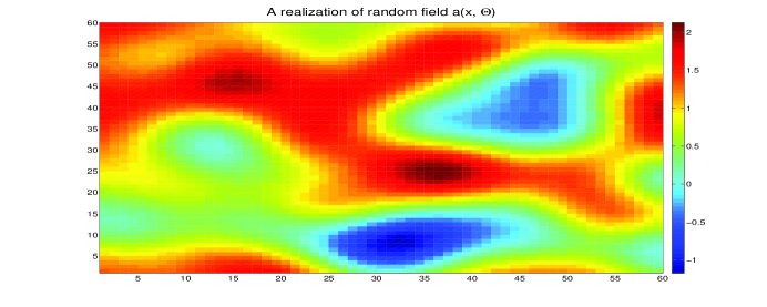
Fig. 1: A realization of random field $a(x,\Theta)$

The stochastic permeability field $k(x,\Theta)$ is given by $k(x,\Theta)=\exp\big{(}a(x,\Theta)\big{)}$, where $a(x,\Theta)$ is characterized by the covariance function $\mbox{cov}[a]$ defined in (41), whose parameters are defined as follows: $\sigma^{2}=1$, $l_{x}=l_{y}=0.1$. We note that the deceay rate of the eigenvalues in the KLE (42) expansion depends inversely on the correlation length and is often used as a guideline to determine the number of terms, $N$ [43]. Here the decay rate is relatively slow and we use 80 terms to represent the random field $a(x,\Theta)$ with a relative error of less than 5%. This implies that $k(x,\Theta)$ is defined in an $80$-dimensional random parameter space, i.e., $N=80$. Fig. 1 depicts a realization of the random field $a(x,\Theta)$. The stochastic field $k(x,\Theta)$ is defined in a $60\times 60$ fine grid. We choose $6\times 6$ coarse grid and apply MMsFEM to compute velocity. The time step is taken to be $0.02$ PVI for discretizing temporal variable.

To demonstrate the efficacy of the proposed method to simulate the stochastic linear two-phase flow system, we compare the performance of several methods: fine-scale mixed finite element method (MFEM) with full random dimensions, MMsFEM on full random dimensions, MMsFEM based on adaptive HDMR, and MMsFEM based on hybrid HDMR. The solution computed by fine-scale MFEM with the full stochastic space is referred to as the reference solution in this paper. To assess the performance of the various MMsFEM and HDMR combinations, we compute the mean and standard deviation (std) for the quantifies of interest from the two-phase flow model, such as saturation and water-cut. Since the random field in the example does not have strong non-local features, the local MMsFEM (L-MMsFEM) generally gives an accurate approximation [25], and it is used in this example. To choose the most active random dimensions for adaptive HDMR and hybrid HDMR, we choose a threshold constant $\zeta=0.9$ and use criteria (15). This approach produces $31$ most active dimensions. The Smolyak sparse-grid collocation method with level $2$ is used to tackle the stochastic space. We evaluate the flow model’s outputs at the collocation points and use the associated weights to compute the mean and standard deviation of the outputs. Table 1 lists the number of deterministic models to be solved for the above four different methods. From the table, we see that MFEM on full random dimensions needs to compute the largest number of deterministic models (fine-scale models), MMsFEM based on hybrid HDMR needs to compute the smallest number of deterministic models (coarse-scale models). This means that MMsFEM based on hybrid HDMR significantly reduces the computational complexity.

Table 1: number of deterministic models for the different methods

methods	number of deterministic models
MFEM on full random dim.	12961 fine-scale models
MMsFEM on full random dim	12961 coarse-scale models
MMsFEM based on adaptive HDMR	6446 coarse-scale models
MMsFEM based on hybrid HDMR	2231 coarse-scale models

Fig. 2 shows the point-wise mean of the saturation field at $\mbox{PVI}=0.4$. In this figure, we observe that both L-MMsFEM based on the hybrid HDMR and L-MMsFEM based on the adaptive HDMR are almost identical to the reference mean computed by fine-scale MFEM on full random dimensions. Fig. 3 illustrates the point-wise standard deviation of saturation at $\mbox{PVI}=0.4$ and leads to four observations: (1) Compared with reference standard deviation, the approximations of standard deviation by the three multiscale models (L-MMsFEM on full random dim., L-MMsFEM based on hybrid HDMR and L-MMsFEM based on adaptive HDMR) are good; (2) L-MMsFEM on full random dim. renders better approximation for standard deviation than L-MMsFEM based on truncated HDMR techniques; (3) L-MMsFEM based on hybrid HDMR gives almost the same standard deviation as the L-MMsFEM based on adaptive HDMR; (4) The variance mostly occurs along the advancing water front, and where the front interacts with the domain boundary. Fig. 4 shows the mean of water-cut curves, which are all nearly identical. This demonstrates that a good approximation has been achieved. Fig. 5 shows the standard deviation of water-cut curves from the four different methods. Here, we see that both L-MMsFEM based on hybrid HDMR and L-MMsFEM based on adaptive HDMR produce a very good approximation for the standard deviation at most time instances. The standard deviation of the water-cut curve from L-MMsFEM based on hybrid HDMR is almost identical to the standard deviation of water-cut curve from L-MMsFEM based on adaptive HDMR.

Next we discuss the relative errors of the domain integrated mean and standard deviation. Let $S_{r}$/$W_{r}$, $S_{ms,f}$/$W_{ms,f}$, $S_{ms,aH}$/$W_{ms,aH}$ and $S_{ms,hH}$/$W_{ms,hH}$ be the saturation/water-cut using MFEM on full random dimensions, MMsFEM on full random dimensions, MMsFEM based on adaptive HDMR and MMsFEM based on hybrid HDMR, respectively. Then we define the relative errors of saturation mean and saturation standard deviation between $S_{r}$ and $S_{ms,f}$ as following,

$$\mathcal{E}_{ms}^{m}(S)=\frac{\|E[S_{r}](x)-E[S_{ms,f}](x)\|_{L^{1}(D)}}{\|E[S_{r}](x)\|_{L^{1}(D)}},\quad\mathcal{E}_{ms}^{std}(S)=\frac{\|\sigma[S_{r}](x)-\sigma[S_{ms,f}](x)\|_{L^{1}(D)}}{\|\sigma[S_{r}](x)\|_{L^{1}(D)}},$$ (43)

where $\sigma$ denotes the standard deviation operation. We can similarly define the relative errors $\mathcal{E}_{aH}^{m}(S)$ and $\mathcal{E}_{aH}^{std}(S)$ between $S_{r}$ and $S_{ms,aH}$, and the relative errors $\mathcal{E}_{hH}^{m}(S)$ and $\mathcal{E}_{hH}^{std}(S)$ between $S_{r}$ and $S_{ms,hH}$. We list these errors on saturation at $0.4$ PVI in Table 2. From the table, we see that L-MMsFEM based on hybrid HDMR gives the same accuracy of mean as L-MMsFEM based on adaptive HDMR. They are both very close to the error of mean by L-MMsFEM on full random dimensions. The relative error of standard deviation by L-MMsFEM based on hybrid HDMR also has a good agreement with that of L-MMsFEM based on adaptive HDMR. The table implies that the errors only from adaptive HDMR and hybrid HDMR are very small. The main source of errors is from spatial multiscale approximation.

Table 2: relative errors of mean and std. on saturation (at 0.4 PVI)

methods	relative error of mean	relative error of std.
L-MMsFEM on full random dim.	1.223540e-002	5.302182e-002
L-MMsFEM based on adaptive HDMR	1.361910e-002	9.389291e-002
L-MMsFEM based on hybrid HDMR	1.361910e-002	9.482789e-002

For water-cut, the relative errors of mean and standard deviation between $W_{r}$ and $W_{ms,f}$ are defined by

$$\mathcal{E}_{ms}^{m}(W)=\frac{\|E[W_{r}](t)-E[W_{ms,f}](t)\|_{L^{2}([0,1]}}{\|E[W_{r}](t)\|_{L^{2}([0,1])}},\quad\mathcal{E}_{ms}^{std}(W)=\frac{\|\sigma[W_{r}](t)-\sigma[W_{ms,f}](t)\|_{L^{2}([0,1])}}{\|\sigma[W_{r}](t)\|_{L^{2}([0,1])}},$$ (44)

where $[0,1]$ is the temporal domain. The relative errors of water-cut, such as $\mathcal{E}_{aH}^{m}(W)$, $\mathcal{E}_{aH}^{std}(W)$, $\mathcal{E}_{hH}^{m}(W)$ and $\mathcal{E}_{hH}^{std}(W)$, are defined in a similar way. We list these relative errors in Table 3. The table shows similar behavior for these methods as was observed in the calculation of saturation mean and saturation standard deviation. The performance of L-MMsFEM based on hybrid HDMR is almost the same as the performance of L-MMsFEM based on adaptive HDMR.

Table 3: relative errors of mean and std. on water-cut

methods	relative error of mean	relative error of std.
L-MMsFEM on full random dim.	1.445791e-002	4.339328e-002
L-MMsFEM based on adaptive HDMR	1.856908e-002	1.006136e-001
L-MMsFEM based on hybrid HDMR	1.856908e-002	1.040452e-001

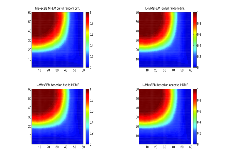
Fig. 2: Point-wise mean of saturation map at PVI=0.4. Top left: MFEM on full random dimensions; Top right: L-MMsFEM on full random dimensions; Bottom left: L-MMsFEM based on hybrid HDMR; Bottom right: L-MMsFEM based on adaptive HDMR

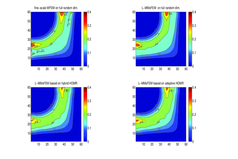
Fig. 3: Point-wise standard deviation of saturation contour at PVI=0.4. Top left: MFEM on full random dimensions; Top right: L-MMsFEM on full random dimensions; Bottom left: L-MMsFEM based on hybrid HDMR; Bottom right: L-MMsFEM based on adaptive HDMR

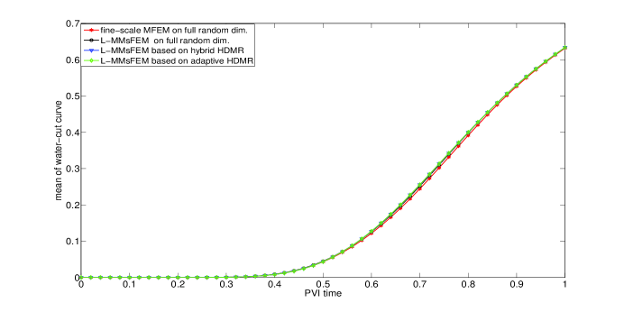
Fig. 4: Mean of water-cut curves

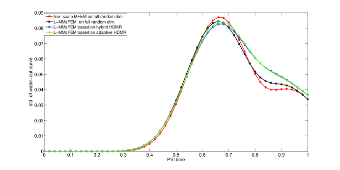
Fig. 5: Standard deviation of water-cut curves

The number of the most active dimensions may have an important impact on both the computational efficiency and solution accuracy. To this end, we investigate the performance for different threshold constants in (15). Specifically, we take $\zeta=0.75$, $0.8$, $0.85$, $0.9$, $0.95$. For these threshold constants, we find that the corresponding number of most active dimensions are $dim(\Theta_{\mathcal{J}})=19$, $22$, $26$, $31$, $41$. Fig. 6 displays the CPU times of L-MMsFEM based on adaptive HDMR and L-MMsFEM based on hybrid HDMR for this set of active dimensions. Here, two observations are important to note: (1) The CPU time of L-MMsFEM based on hybrid HDMR is only a fraction of the CPU time using L-MMsFEM based on adaptive HDMR; (2) As the number of the most active dimensions increases, the CPU time of L-MMsFEM based on hybrid HDMR increases mildly, but the CPU time of L-MMsFEM based on adaptive HDMR increases dramatically. This comparison demonstrates that hybrid HDMR is much more efficient than adaptive HDMR. There are two reasons that adaptive HDMR requires more CPU time: (1) adaptive HDMR needs to solve more deterministic models; (2) to compute the standard deviation (or variance), a large number of stochastic interpolations are involved. Fig. 7 shows the relative errors of mean (left) and standard deviation (right) for saturation at $0.4$ PVI. From the figure, we conclude that increasing the number of the most active dimensions can substantially improve the accuracy of the mean and standard deviation for saturation. We also see that for the saturation approximation the L-MMsFEM based on hybrid HDMR has almost the same accuracy as the L-MMsFEM based on adaptive HDMR. Fig. 8 presents the relative errors of water-cut mean (left) and water-cut standard deviation (right) for the different number of the most active dimensions. From the figure, we observe that the reduction in the error with increasing $dim(\Theta_{\mathcal{J}})$ is smaller for water-cut than for mean saturation. Here, the error from L-MMsFEM is dominating the total error, and hence, is overwhelming the impact of improved accuracy in the HDMR itself.

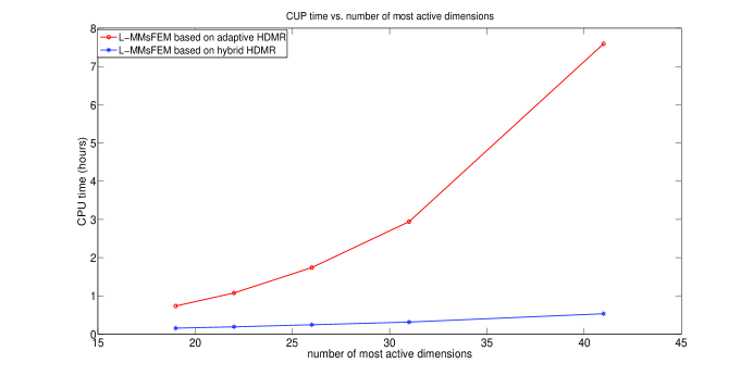
Fig. 6: CPU time for the different number of the most active dimensions, $19,22,26,31,41$.

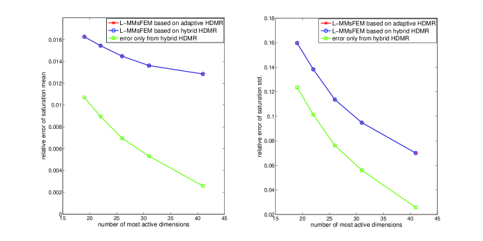
Fig. 7: Relative errors of mean (left) and standard deviation (right) for saturation at $0.4$ PVI.

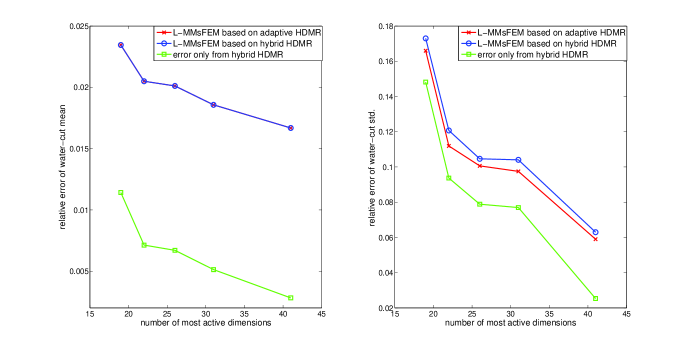
Fig. 8: Relative errors of mean (left) and standard deviation (right) for water-cut.

5.2 Non-linear transport

In this subsection, we consider the two-phase flow system (5) with the mobilities of water and oil defined by nonlinear functions of saturation,

$$\lambda_{w}(S)=S^{2}/\mu_{w},\quad\lambda_{o}(S)=(1-S)^{2}/\mu_{o}.$$

Here $\mu_{w}/\mu_{o}=0.1$, the ratio between viscosity of water and oil. Consequently, the fractional flow function $f_{w}(S)$ of water is given by

$$f_{w}(S)=\frac{S^{2}}{S^{2}+0.1(1-S)^{2}}.$$

This results in a non-linear two-phase flow system.

We again consider the random permeability $k(x,\Theta)=\exp\big{(}a(x,\Theta)\big{)}$. Here the covariance function $\mbox{cov}[a]$ of $a(x,\Theta)$ is defined in (41) with $l_{x}=l_{y}=0.2$ and $\sigma^{2}=1$. The mean of $a(x,\Theta)$ is highly heterogeneous and its map is depicted in Fig. 9 (left). It is actually obtained by extracting and rescaling an SPE 10 [8] permeability field (the $45$-th layer). We truncate the KLE (42) after the first $30$ terms to represent the random field $a(x,\Theta)$ and so the random field $k(x,\Theta)$ is defined in a $30$-dimensional random parameter space. Fig. 9 shows a realization of the random field $a(x,\Theta)$ (right). The stochastic field $k(x,\Theta)$ is defined on a $60\times 60$ fine grid. We choose a $6\times 6$ coarse grid for MMsFEM to compute the velocity. To discretize the temporal variable of the saturation equation, the time step is taken to be $0.01$ PVI.

Fig. 9 shows that the permeability field $k(x,\Theta)$ exhibits some channelized features, which have important an impact on the flow. To achieve accurate simulation results in this setting, limited global information can improve the accuracy [1, 2, 25]. In this subsection, we incorporate the hybrid HDMR technique and the adaptive HDMR technique with both local MMsFEM (L-MMsFEM) and global MMsFEM (G-MMsFEM), and compare the performance of these methods. To obtain the most active random dimensions for the truncated HDMR techniques, we choose a threshold constant $\zeta=0.9$ and use criteria (15). This gives rise to $14$ most active dimensions in the $30$-dim random parameter space. We use the collocation points and weights associated with level $2$ Smolyak sparse-grid collocation to compute the mean and standard deviation.

Fig. 10 shows the point-wise mean of saturations at $0.4$ PVI for different methods. We can clearly see that G-MMsFEM on full random dimensions yields the best approximation to the reference solution, which is given by fine-scale MFEM on full random dimensions. The figure also shows that the multiscale methods with the truncated HDMR techniques provide good approximations. Fig. 11 describes the point-wise standard deviation of saturation at $0.4$ PVI for those different methods. Based on the figure, we make two observations: (1) the largest variance occurs around the water front; (2) the hybrid HDMR technique gives almost the same standard deviation map as the adaptive HDMR technique. We note that these observations are consistent with those of Section 5.1. We also compute the water-cut curves for the different methods. To minimize overlap in the visualization, we only present the water-cut curves for four methods: MFEM on full random dim., G-MMsFEM on full random dim., G-MMsFEM based on adaptive HDMR and G-MMsFEM based on hybrid HDMR. Fig. 12 shows the mean of the water-cut curves for the four methods. Here, the four curves overlap each other at almost all times. We note that there exists a small fluctuation right after the water breaks through. The reason may be that the value of water-cut changes sharply right after water break-through time. The standard deviation of the water-cut curves for the four methods are illustrated in Fig. 13. From the figure, we find that the variance of water-cut rises rapidly at the break-through time, and has a small number of peaks that are likely related to the dominant channelized flow paths in the underlying mean permeability field.

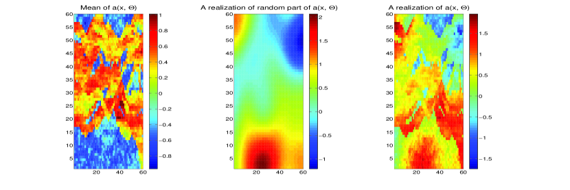
Fig. 9: A realization of random field $a(x,\Theta)$

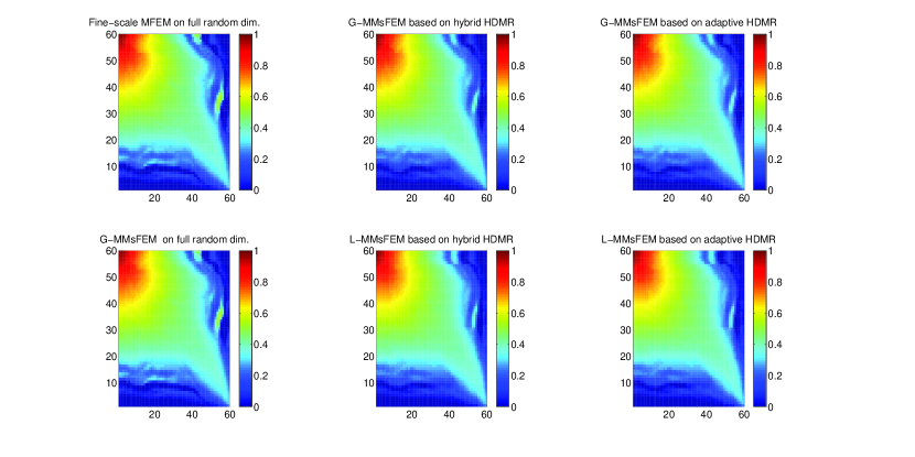
Fig. 10: Point-wise mean of saturations at $0.4$ PVI for different methods

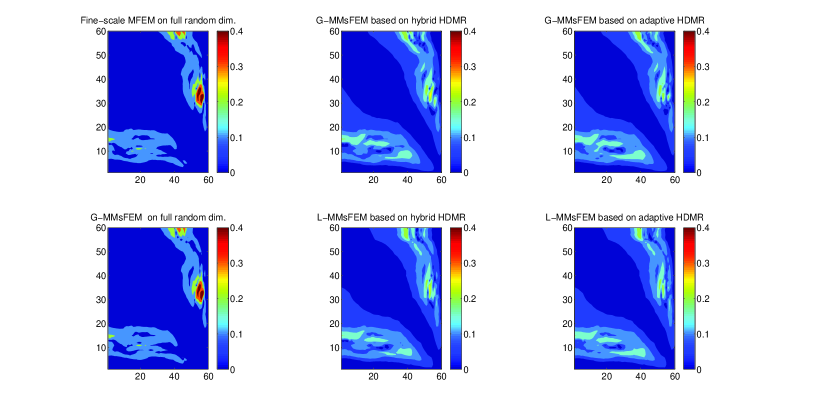
Fig. 11: Point-wise standard deviation of saturations at $0.4$ PVI for different methods

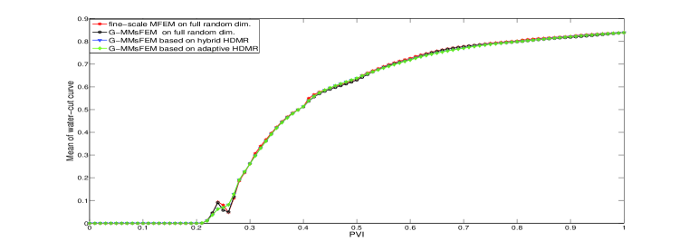
Fig. 12: Mean of water-cut curves for MFEM on full random dim., G-MMsFEM on full random dim., G-MMsFEM based on adaptive HDMR and G-MMsFEM based on hybrid HDMR

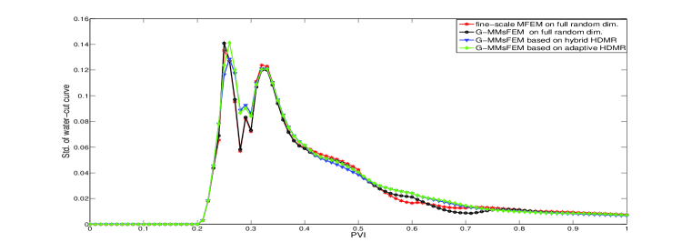
Fig. 13: Standard deviation of water-cut curves for MFEM on full random dim., G-MMsFEM on full random dim., G-MMsFEM based on adaptive HDMR and G-MMsFEM based on hybrid HDMR

In order to carefully measure the differences caused by L-MMsFEM and G-MMsFEM when integrated with adaptive HDMR and hybrid HDMR, we follow the procedure outlined in Subsection 5.1 and compute the relative errors between the reference solution and the solutions of the various coarse models (MMsFEM with (or without) HDMR techniques). As before, the reference solution is solved by fine-scale MFEM on full random dimensions. The relative errors of saturation and water-cut are defined similarly to (43) and (44), respectively. Table 4 and 5 list the relative errors of mean and standard deviation for saturation at $0.4$ PVI and water-cut, respectively. Examining this table, we note: (1) limited global information can enhance the accuracy of MMsFEM; (2) the results by adaptive and hybrid HDMR are very close to each other.

Table 4: relative errors of mean and std. on saturation (at 0.4 PVI)

methods	relative error of mean	relative error of std.
L-MMsFEM on full random dim.	4.170726e-002	1.545560e-001
G-MMsFEM on full random dim.	8.950902e-003	4.027147e-002
L-MMsFEM based on adaptive HDMR	4.788991e-002	2.051337e-001
G-MMsFEM based on adaptive HDMR	3.283281e-002	1.608348e-001
L-MMsFEM based on hybrid HDMR	4.788991e-002	2.013145e-001
G-MMsFEM based on hybrid HDMR	3.283281e-002	1.520236e-001

Table 5: relative errors of mean and std. on water-cut

methods	relative error of mean	relative error of std.
L-MMsFEM on full random dim.	1.320466e-002	8.836354e-002
G-MMsFEM on full random dim.	8.000854e-003	4.298053e-002
L-MMsFEM based on adaptive HDMR	1.423242e-002	1.352706e-001
G-MMsFEM based on adaptive HDMR	1.162734e-002	1.212131e-001
L-MMsFEM based on hybrid HDMR	1.423242e-002	1.447519e-001
G-MMsFEM based on hybrid HDMR	1.162734e-002	1.248755e-001

Finally we examine the efficiency for the different approaches. To this end, we record the CPU time for the seven different methods: fine-scale MFEM on full random dimensions, L-MMsFEM on full random dimensions, G-MMsFEM on full random dimensions, L-MMsFEM based on adaptive HDMR, G-MMsFEM based on adaptive HDMR, L-MMsFEM based on hybrid HDMR and G-MMsFEM based on hybrid HDMR. Fig. 14 shows the CPU time for the seven different approaches. Here it is apparent that the approaches based on hybrid HDMR need the least CPU time and achieve the best efficiency. The CPU time of hybrid HDMR is only a fraction, about a third, of the CPU time of adaptive HDMR. Moreover, this speedup was shown earlier to increase quickly with the number of most active dimensions. Comparing the performance of the local and global MMsFEM based methods, we find that for each HDMR technique, the CPU time of G-MMsFEMs is only slightly larger than the CPU time of L-MMsFEM. For adaptive HDMR, a significant amount of CPU time is spent in computing variance. However, computation of the variance in hybrid HDMR is straightforward and requires very little CPU time. This is an important advantage of the hybrid HDMR approach.

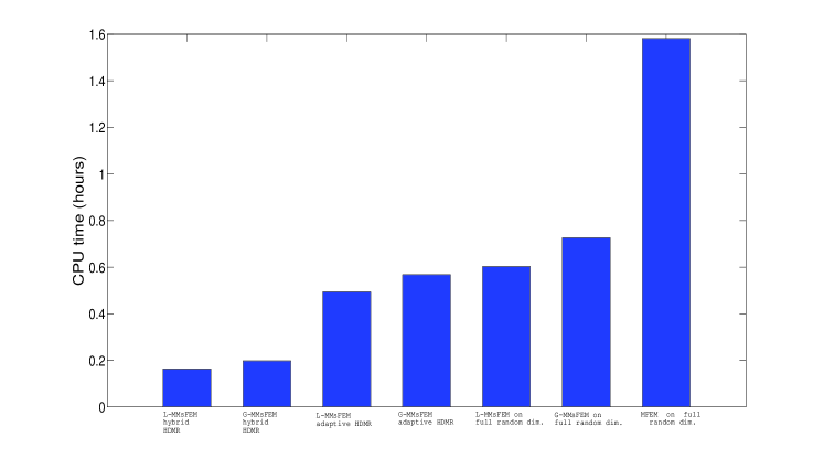
Fig. 14: CPU time for different approximation models, using 14 most active dimensions for the truncated HDMR techniques.

6 Conclusions

In this paper, we presented a general framework for high-dimensional model representations (HDMRs), and proposed a hybrid HDMR technique in combination with a mixed multiscale finite element method (MMsFEM) to simulate two-phase flow through heterogeneous porous media. The hybrid HDMR technique decomposes a high-dimensional stochastic model into a moderate-dimensional stochastic model and a few one-dimensional stochastic models. An optimization criteria was developed that ensures a specified percentage of the total variance is present in the most active dimensions (i.e., the moderate-dimensional stochastic model). In addition, we demonstrated that combining an MMsFEM with hybrid HDMR could significantly reduce the original model’s complexity in both the resolution of the physical space and the high-dimensional stochastic space. We also presented MMsFEM based on adaptive HDMR, which has been widely used in stochastic model reduction. Compared with adaptive HDMR, the hybrid HDMR is much more efficient and retains the same (or better) accuracy. To capture strong non-local features in the multiscale models, we have incorporated important global information into the multiscale computation. This can improve the approximation accuracy of the proposed coarse multiscale models. We carefully analyzed the proposed MMsFEM using HDMR techniques and discussed both the computational efficiency and approximation errors. The MMsFEM based on HDMR techniques was applied to two-phase flows in heterogeneous random porous media. Both linear and non-linear saturation dependencies of the mobility were considered. The simulation results confirmed the performance of the proposed approaches.

Appendix A proof of Theorem 3

For the proof, we need to calculate the HDMR components in $f^{anova}(\Theta)$. By definition, we derive the term $\hat{f}^{anova}(\Theta_{\mathcal{J}})$ as follows,

$$\begin{split}\hat{f}^{anova}(\Theta_{\mathcal{J}})&=\widehat{\mathrm{P}}_{\mathcal{J}}f^{cut}=\int_{I^{N-J}}f^{cut}(\Theta)\Pi_{i\notin\mathcal{J}}d\mu_{i}(\theta_{i})\\ &=\int_{I^{N-J}}\hat{f}^{cut}(\Theta_{\mathcal{J}})\Pi_{i\notin\mathcal{J}}d\mu_{i}(\theta_{i})+\sum_{i\in\{1,\cdots,N\}\setminus\mathcal{J}}\int_{I^{N-J}}f_{i}^{cut}(\theta_{i})\Pi_{i\notin\mathcal{J}}d\mu_{i}(\theta_{i})\\ &=\hat{f}^{cut}(\Theta_{\mathcal{J}})+\sum_{i\in\{1,\cdots,N\}\setminus\mathcal{J}}E[f_{i}^{cut}].\end{split}$$ (45)

We define $f_{0}^{anova}=E[f^{cut}]$. Then for any $i\in\{1,\cdots,N\}\setminus\mathcal{J}$, we have

$$\begin{split}&f_{i}^{anova}(\theta_{i})=\int_{I^{N-1}}f^{cut}(\Theta)\Pi^{N}_{\begin{subarray}{c}s=1\\ s\neq i\end{subarray}}d\mu_{s}(\theta_{s})-f_{0}^{anova}\\ &=\int_{I^{N-1}}\hat{f}^{cut}(\Theta_{\mathcal{J}})\Pi^{N}_{\begin{subarray}{c}s=1\\ s\neq i\end{subarray}}d\mu_{s}(\theta_{s})+\sum_{j\in\{1,\cdots,N\}\setminus\mathcal{J}}\int_{I^{N-1}}f_{j}^{cut}(\theta_{j})\Pi^{N}_{\begin{subarray}{c}s=1\\ s\neq i\end{subarray}}d\mu_{s}(\theta_{s})-f_{0}^{anova}\\ &=f_{i}^{cut}(\theta_{i})+E[\hat{f}^{cut}]+\sum_{\begin{subarray}{c}j\in\{1,\cdots,N\}\setminus\mathcal{J}\\ j\neq i\end{subarray}}E[f_{j}^{cut}]-f_{0}^{anova}\\ &:=f_{i}^{cut}(\theta_{i})+C_{i}.\end{split}$$ (46)

It is obvious that $E[f_{i}^{anova}]=0$ by (46). Consequently, it follows that by (45),

$$E[f^{anova}]=E[\hat{f}^{anova}]=E[\hat{f}^{cut}]+\sum_{i\in\{1,\cdots,N\}\setminus\mathcal{J}}E[f_{i}^{cut}]=E[f^{cut}].$$

This proves the equality (25). For ANOVA-HDMR, we note that

$$\begin{split}\mbox{Var}[f^{anova}]&=\|f^{anova}\|^{2}_{\mathcal{F}}=\|\hat{f}^{anova}\|_{\mathcal{F}}^{2}+\sum_{i\in\{1,\cdots,N\}\setminus\mathcal{J}}\|f_{i}^{anova}\|_{\mathcal{F}}^{2}\\ &=\mbox{Var}[\hat{f}^{anova}]+\sum_{i\in\{1,\cdots,N\}\setminus\mathcal{J}}\mbox{Var}[f_{i}^{anova}]\\ &=\mbox{Var}[\hat{f}^{cut}]+\sum_{i\in\{1,\cdots,N\}\setminus\mathcal{J}}\mbox{Var}[f_{i}^{cut}],\end{split}$$ (47)

where equations (45) and (46) have been used in the last step. Further, by equations (45) and (46) we have

$$\begin{split}f^{cut}(\Theta)&=\hat{f}^{cut}(\Theta_{\mathcal{J}})+\sum_{i\in\{1,\cdots,N\}\setminus\mathcal{J}}f_{i}^{cut}(\theta_{i})\\ &=\hat{f}^{anova}(\Theta_{\mathcal{J}})-\sum_{i\in\{1,\cdots,N\}\setminus\mathcal{J}}E[f_{i}^{cut}]+\sum_{i\in\{1,\cdots,N\}\setminus\mathcal{J}}\big{(}f_{i}^{anova}(\theta_{i})-C_{i}\big{)}\\ &=f^{anova}(\Theta)-\bigg{(}\sum_{i\in\{1,\cdots,N\}\setminus\mathcal{J}}\big{(}E[f_{i}^{cut}]+C_{i}\big{)}\bigg{)}.\end{split}$$ (48)

This implies that $\mbox{Var}[f^{cut}]=\mbox{Var}[f^{anova}]$. Hence the proof is completed.

References

- [1] J.E. Aarnes, On the use of a mixed multiscale finite element method for greater flexibility and increased speed or imporved accuracy in reservoir simulation. Multiscale Model. Simul., 2 (2004), pp.421–439.
- [2] J. E. Aarnes, Y. Efendiev and L. Jiang, Mixed multiscale finite element methods using limited global information, Multiscale Model. Simul., 7 (2008), pp. 655–676.
- [3] T. Arbogast, Implementation of a locally conservative numerical subgrid upscaling scheme for two-phase Darcy flow, Comput. Geosci., 6 (2002), pp. 453–481.
- [4] M. Arnst, R. Ghanem, Probabilistic equivalence and stochastic model reduction in multiscale analysis, Comput. Methods Appl. Mech. Engrg., 197 (2008), pp. 3584—3592.
- [5] I. Babuka, F. Nobile and G. Zouraris, A stochastic collocation method for elliptic partial differential equations with random input data, SIAM J. Numer. Anal., 45 (2007), pp. 1005–1034.
- [6] V. Barthelmann, E. Novak and K. Ritter, High dimensional polynomial interpolation on sparse grids, Advanced in Compuational Mathematics 12 (2000), pp. 273–288.
- [7] Z. Chen and T. Y. Hou, A mixed multiscale finite element method for elliptic problems with oscillating coefficients, Math. Comp., 72 (2002), pp. 541–576.
- [8] M. Christie and M. Blunt, Tenth SPE comparative solution project: A comparison of upscaling techniques, SPE Reser. Eval. Eng., 4 (2001), pp. 308–317.
- [9] R.I. Cukier, J.H. Schaibly, and K.E. Shuler, Study of the sensitivity of coupled reaction systems to uncertainties in rate coefficients. III. Analysis of the approximations, Journal of Chemical Physics, 63 (1975), pp. 1140–1149.
- [10] W. E and B. Engquist, The heterogeneous multi-scale methods, Comm. Math. Sci., 1 (2003), pp. 87–133.
- [11] Y. Efendiev, J. Galvis and X. Wu, Multiscale finite element methods for high-contrast problems using local spectral basis functions, J. Comput. Phys., 230 (2011), pp. 937-955.
- [12] Y. Efendiev and T. Y. Hou, Multiscale Finite Element Methods: Theory and Applications, Springer, 2009.
- [13] O. G. Ernst, C. E. Powell, D. J. Silvester, and E. Ullmann, Efficient solvers for a linear stochastic Galerkin mixed formulation of diffusion problems with random data, SIAM J. Sci. Comput., 31 (2009), pp. 1424 C1447.
- [14] G.S. Fishman, Monte Carlo, Concepts, Algorithms and Applications, Springer-Verlag, New York, 1996.
- [15] B. Ganapathysubramanian and N. Zabaras, A stochastic multiscale framework for modeling flow through random heterogeneous prous media, J. Comput. Physics., 228 (2009), pp.591–618.
- [16] B. Ganis, I. Yotov and M. Zhong, A stochastic mortar mixed finite element method for flow in porous media with multiple rock types, SIAM J. Sci. Comp., 33 (2011), pp. 1439–1474.
- [17] Z. Gao and J. S. Hesthaven, On ANOVA expansion and strategies for choosing the anchor point, Applied Mathematics and Computation, 217 (2010), pp. 3274–3285.
- [18] T. Gerstner and M. Griebel, Numerical integration using sparse grids, Numerical Algorithm 18 (1998), pp. 209–232.
- [19] R. Ghanem and P. D. Spanos, Stochastic finite elements: a spectral approach, Springer-Verlag, 1991.
- [20] V. Ginting, A. Malqvist and M. Presho, A novel method for solving multiscale elliptic problems with randomly perturbed data, Multiscale Model. Simul., 8 (2010), pp. 977–996.
- [21] W. J. Gordon, Distributive lattices and the approximation of multivariate functions, in: Proc. Symp. Approximation with Spectial Emphasis on Spline Functions (edited by I.J. Schoenberg), Academic Press, New York, 1969.
- [22] M. Griebel and M. Holtz, Dimension-wise integration of high-dimensional functions with applications to finance, Journal of Complexity, 26 (2010), pp. 455–489.
- [23] T. Hughes, G. Feijoo, L. Mazzei, and J. Quincy, The variational multiscale method - a paradigm for computational mechanics, Comput. Methods Appl. Mech. Engrg, 166 (1998), pp. 3–24.
- [24] P. Jenny, S. H. Lee, and H. Tchelepi, Multi-scale finite volume method for elliptic problems in subsurface flow simulation, J. Comput. Phys., 187 (2003), pp. 47–67.
- [25] L. Jiang, Y. Efendiev and I. Mishev, Mixed multiscale finite element methods using approximate global information based on partial upscaling, Comput. Geosci., 14 (2010), pp. 319–341.
- [26] L. Jiang, I. Mishev, Y. Li, Stochastic mixed multiscale finite element methods and their applications in reandom porous media, Comput. Methods Appl. Mech. Engrg., 119(2011), pp. 2721–2740.
- [27] L. Jiang and M. Presho, A resourceful splitting technique with applications to deterministic and stochastic multiscale finite element methods, Multiscale Model. Simul., 10 (2012), pp. 954–985.
- [28] F. Y. Kuo, I. H. Sloan, G. W. Wasilkowski, and H. Woźniakowski, On decompositions of multivariate functions, Math. Comp., 79 (2009), pp. 953–966.
- [29] O. P. LeMaître and O. M. Knio, Spectral methods for uncertainty quantification: with applications to computational fluid dynamics, Springer–New York, 2010.
- [30] G. Lin and A. Tartakovsky, Numerical studies of three-dimensional stochastic Darcys equation and stochastic advection-diffusion-dispersion equation, Journal of Scientific Computing, 43 (2010), pp. 92–117.
- [31] M. Loève, Probability Theory (4th ed.), Springer Verlag, Berlin, 1977.
- [32] X. Ma and N. Zabaras, A adaptive high-dimensional stochastic model represenation technique for the solution of stochastic partial differential equations, J. Comput. Phys., 229 (2010), pp. 3884–3915.
- [33] X. Ma and N. Zabaras, A stochastic mixed finite element heterogeneous multiscale method for flow in porous media, J. Comput. Phys., 230 (2011), pp. 4696–4722.
- [34] H. G. Matthies and A. Keese Galerkin methods for linear and nonlinear elliptic stochastic partial differential equations, Comput. Methods Appl. Mech. Engrg., 194 (2005), pp.1295–1331.
- [35] N.C. Nguyen, A multiscale reduced-basis method for parameterized elliptic partial differential equations with multiple scales, J. Comput. Phys., 227 (2008), pp. 9807–9822.
- [36] F. Nobile, R. Tempone and C. G. Webster, A sparse grid stochastic collocation method for partial differential equations with random input data, SIAM J. Numer. Anal., 46 (2008), pp. 2309–2345.
- [37] H. Rabitz, ö. F. Allis, General foundations of high-dimensional model representations, Journal of Mathematical Chemistry 25 (1999), pp. 197–233.
- [38] H. Rabitz, ö. F. Allis, J. Shorter and K. Shim, Efficient input-output model represenation, Comput. Phys. Commun., 117 (1999), pp. 11–20.
- [39] G. Rozza, D. B. P. Huynh and A. T. Patera, Reduced basis approximation and a posteriori error estimation for affinely parametrized elliptic coercive partial differential equations, Arch. Comput. Methods Eng. 15 (2008), pp. 229–275.
- [40] S. Smolyak, Quadrature and interpolation formulas for tensor products of certain classes of functions, Soviet Math. Dokl. 4, 1963, pp. 240–243.
- [41] J. Wei, G. Lin, L. Jiang and Y. Efendiev, ANOVA-based mixed multiscale finite element method and applications in stochastic two-phase flows, submitted, 2013.
- [42] D. Xiu and Jan S. Hesthaven, High-order collocation methods for differential equations with random inputs, SIAM J. Sci. Comput. 27 (2005), pp. 1118-1139.
- [43] D. Xiu, Numerical Methods for Stochastic Computations: A Spectral Approach, Princeton University Press, Princeton, NJ (2010).
- [44] X. Frank Xu, A multiscale stochastic finite element method on elliptic problems involving uncertainties, Comput. Methods Appl. Mech. Engrg., 196 (2007), pp.2723–2736.
- [45] X. Frank Xu, Stochastic computation based on orthogonal expansion of random fields, Comput. Methods Appl. Mech. Engrg., 200 (2011), pp. 2871–2881.
- [46] X. Frank Xu, Quasi-weak and weak formulation of stochastic finite elements on static and dynamic problems a unifying framework, Probabilistic Engineering Mechanics, 28 (2012), pp. 103–109.
- [47] X. Yang, M. Choi, G. Lin and G. E. Karniadakis, Adaptive ANOVA decompsotion of stochastic incompressible and compressible flows, J. Comput. Phys., 2011, doi:10.1016/j.jcp.2011.10.028.
- [48] D. Zhang, L. Li and H. Tchelepi, Stochastic formulation for uncertainty analysis of two-phase flow in heterogeneous reservoirs. SPE Journal 5 (2000), pp. 60–70.